Approximations for the Moments of Nonstationary and State Dependent Birth-Death Queues

Abstract

In this paper we propose a new method for approximating the nonstationary moment dynamics of one dimensional Markovian birth-death processes. By expanding the transition probabilities of the Markov process in terms of Poisson-Charlier polynomials, we are able to estimate any moment of the Markov process even though the system of moment equations may not be closed. Using new weighted discrete Sobolev spaces, we derive explicit error bounds of the transition probabilities and new weak a priori estimates for approximating the moments of the Markov processs using a truncated form of the expansion. Using our error bounds and estimates, we are able to show that our approximations converge to the true stochastic process as we add more terms to the expansion and give explicit bounds on the truncation error. As a result, we are the first paper in the queueing literature to provide error bounds and estimates on the performance of a moment closure approximation. Lastly, we perform several numerical experiments for some important models in the queueing theory literature and show that our expansion techniques are accurate at estimating the moment dynamics of these Markov process with only a few terms of the expansion.

Keywords: Multi-Server Queues, Spectral-Galerkin method, Discrete approximation, Unbounded domain, Abandonment, Time-Varying Rates, Birth-Death Processes, Poisson-Charlier Polynomials.

AMS subject classification: NNXMM.

1 Introduction

Birth-Death Markov processes are very important modeling tools in engineering, operations research, mathematics, physics, and a variety of other fields. The development of Markovian stochastic models has made a profound impact on the way we understand complex dynamics in these fields of study. One particular way to explore the dynamics of these processes that transcends a particular application setting is to study the behavior of the transition probabilities and the state probabilities, which provide the entire distribution of the process for all time points of interest. However, an explicit study of the transition probabilities or state probabilities has often eluded researchers since the transition or state probabilities do not have explicit solutions in general with some exceptions in some very special cases. Moreover, when analyzing large models such as large scale service systems or moderately sized queueing networks a full understanding of the transition or state probabilities in their explicit form is rather intractable in both a mathematical and numerical sense.

Thus, many researchers have spent considerable effort in trying to develop ways of understanding the moments of Markovian birth-death processes. Moments like the mean and variance can provide considerable insight into understanding the “typical” stochastic behavior of the system. However, a full understanding of the moments also is quite difficult. One main difficulty that is often encountered is that the system of differential equations describing the moments of the birth-death process might not be closed. This means that it is necessary that one know the true distribution of the Markov process or at least its higher moments in order to compute the lower moments of the stochastic process.

One common approach to circumvent the lack of closure is to apply asymptotic methods such as heavy traffic limit theorems. Such results scale or speed up the rates of the stochastic process in order to simplify the stochastic analysis of the Markov process, see for example Massey [12] and Mandelbaum et al [11]. However, these methods are asymptotic and therefore only apply when the stochastic processes rates are infinite or very large. They do not apply directly to a process that has moderate rates. Moreover, currently, there are no methods to determine how close our nonstationary approximations are to the true stochastic process for a particular finite rate.

An alternative method for computing the moments of the Markov process is to apply what are known as closure approximations to the stochastic process under consideration. Closure approximations attempt to intelligently approximate the distribution of the Markov process and use this approximate distribution to estimate the moments of the stochastic process. By using the closure approximation, it should be simple to calculate the moment dynamics and perhaps more importantly, the moment dynamics should be close to the true dynamics of the original process. See for example Krishnarajah et al [9, 10] in the epidemic process setting and Rothkopf et al [21], Clark [2], and Taaffe et al [22] in the queueing process setting.

A more recent method developed by Massey and Pender [13, 14, 15] is to use Hermite polynomial expansions to approximate the distribution of the queue length process. Taking two or three terms of the expansion works quite well. Since the Hermite polynomials are orthogonal to the Gaussian distribution, which has support on the entire real line, these Hermite polynomial chaos expansions do not take into account the discreteness of the queueing process and the fact that the queueing process is non-negative. Work by Pender [20] uses Laguerre polynomials, which are orthogonal with respect to the gamma distribution on the positive real line, but also ignores the discrete nature of the queueing process. Lastly, Pender [19] provides a Poisson-Charlier expansion for the queue length distribution, however, this work does not prove error bounds for the method and nor does it expand the transition or state probabilities, which we will show is much easier to do. For the continuous distributions like the Hermite and Laguerre it is also quite difficult to prove error bounds on these approximations due to the discrete nature of the queueing process. Therefore, in the context of queueing theory, it is still an open problem to develop closure methods using a discrete reference distribution with provable error bounds for the truncation error.

In this paper, we study one dimensional birth-death models that have nonstationary as well as non-trivial state dependent rates. To develop approximations for the moments and the state probabilities, we use the Poisson-Charlier polynomials to expand the state probabilities of the Markov process in terms of a Poisson reference distribution. This Poisson representation of the transition probabilities is quite natural since a linear birth-death process such as an infinite server queue, has a Poisson distribution when initialized at zero or with a Poisson distribution. Therefore, the terms that serve to correct the true distribution from the Poisson reference distribution can be written explicitly in terms of integrals with respect to the Poisson distribution, which is quite simple. In addition, we should expect that processes that are close to an infinite server queue, should also be approximated quite well with a small number of terms. Moreover, the Poisson reference distribution also allows us to derive explicit approximations for many important stochastic models in the operations research literature such as the nonstationary Erlang-A model, nonstationary Erlang loss model, and even some quadratic birth-death models that are relevant in the applied probability literature. This is because we are able to explicit calculate the rate functions that appear in the functional forward equations using the discrete representation of the incomplete gamma function.

Our approach, which is similar to the spectral Galerkin method of Wulkow [23, 24], later developed by Deuflhard et al [3], and independently by Engblom [5, 6], not only exploits the properties of the Poisson distribution, but also allows us to derive explicit bounds for the transition probabilties and weak a priori estimates for estimating the moments of our approximation method. These bounds and estimates help us understand how many terms we might need to approximate the moments of our birth-death process with good accuracy. Moreover, we can show that as we add more terms to the expansion, the approximate transition probabilities and the moments of the birth-death model converge to the true transition probabilties and moments of the underlying Markov process. However, unlike their continuous counterparts, discrete orthogonal polynomials such as the Poisson-Charlier and their properties are much less studied. This forces us to define new weighted Sobolev spaces to analyze the convergence of our discrete closure approximation. These Sobolev spaces allow us to prove spectral convergence of the method, with error estimates decaying faster than any inverse power of the expansion order $N$, and also allow us to prove that the moments converge by adding more terms to the approximation of the transition probabilities.

Contributions to Literature

In this work we make the following contributions:

• We expand the state probabilities of one-dimensional birth-death Markov processes in terms of Poisson-Charlier polynomials.

• We prove the convergence of the state probabilities and the moments of one-dimensional birth-death Markov processes as we add more terms to the Poisson-Charlier expansion by developing the appropriate Sobolev sequence spaces.

• We derive explicit approximations of several stochastic models and show that a small number of terms is needed to capture important moment behavior of these models. We also show numerically that these explicit approximatons are quite accurate at describing the moment dynamics of the underlying Markov process.

Organization of Paper

The rest of the paper is organized as follows. In Section 2, we introduce the nonstationary and state dependent birth death model that we consider for the remainder of the paper. In Section 3, we introduce the Poisson-Charlier expansion method that we use in the paper and describe the new sequence spaces that are needed to prove convergence of our method. In Section 4 we derive explicit approximations for two important stochastic models using the zeroth order and first order approximations for the transition probabilities. In Section 5, we provide extensive numerical results illustrating the power of our method. Lastly, in the Appendix, we provide the proofs for the explicit approximations that are presented in the paper and provide a brief summary of Poisson-Charlier polynomials and spectral approximations.

2 Nonstationary Birth-Death Model

In this section, we give a description of the birth-death model that is under consideration. Birth-death processes are very important processes in the stochastic community. They arise in variety of applications from queueing theory, chemical reaction networks, neuroscience, and healthcare modelling. Thus, it is important to have a good understanding of the dynamics of these models. In addition, in all of these applications, it is also very important to understand the nonstationary and state dependent aspects of these models. Nonstationary and state dependent dynamics are prevalent in our society, especially in a queueing context, where arrivals of customers is almost never stationary and often depend substantially on the size of the queue.

We consider a continuous time one-dimensional nonhomogeneous birth-death process (BDP) $Q(t)$, $t\geq 0$ on the state space $\mathbf{Z}_{+}=\{0,1,2,\ldots\}$ with time dependent and state dependent rate functions. The rate function for the birth process is denoted by $\lambda_{x}(t)$ and the rate functions for the death process are denoted by $\mu_{x}(t)$, $t\geq 0$, $x\in\mathbf{Z}_{+}$. Moreover, we have that

$$\mathbb{P}(Q(t+h)=j|Q(t)=i)=\begin{cases}\lambda_{i}(t)\cdot h+o(h)&\mbox{if }j\mbox{ = }i+1,\\ \mu_{i}(t)\cdot h+o(h)&\mbox{if }j\mbox{ = }i-1,\\ 1-\lambda_{i}(t)\cdot h-\mu_{i}(t)\cdot h+o(h)&\mbox{if }j\mbox{ = }i,\\ o(h)&\mbox{if }|i-j|>1.\end{cases}$$ (2.1)

It is assumed that the time interval $h>0$ is sufficiently small to eliminate the possibility of multiple events occurring in the same interval. We also denote $o(h)=o_{i}(t,h)$, $i\in\mathbf{Z}_{+}$ such that

$$\lim_{h\to 0}\frac{\sup_{i}\ o_{i}(t,h)}{h}=0.$$ (2.2)

Thus, we define the transition probabilities and the state probabilities respectively as

$$p_{ij}(s,t)=\mathbb{P}(Q(t)=j|Q(s)=i),$$ (2.3)

and

$$p_{i}(t)=\mathbb{P}(Q(t)=i|Q(0)=0).$$ (2.4)

If we let $\mathbf{p(t)}\equiv\{p_{0}(t),p_{1}(t),....p_{\infty}(t)\}$ and we let $\mathcal{A}(t)$ be the matrix induced by (2.1), then we have that

$$\raisebox{0.9pt}{$\stackrel{{\scriptstyle\bullet}}{{\mathbf{p}}}$}(t)=\mathcal{A}(t)\mathbf{p}.$$ (2.5)

We assume that the rates of birth and death are given by the transition probabilities of a Markov chain. Mathematically, this means that the changes in the system in a small time interval are determined by the following transition probabilities

$$\mathbb{P}\{\Delta Q(t+\Delta t)=1\} \equiv \psi_{\alpha}(t,Q(t))\cdot\Delta t$$

$$\mathbb{P}\{\Delta Q(t+\Delta t)=-1\} \equiv \psi_{\delta}(t,Q(t))\cdot\Delta t$$

Brémaud [1, §8.4.3] gives verifiable conditions for non-explosion of the birth and death generator. Typically in the physical or chemical literature the functions $\psi_{\alpha}$ and $\psi_{\delta}$ are polynomials functions of the state $Q(t)$. Although they may be non-linear, they are smooth functions of the state process. However, in fields such as queueing theory, these functions can be nonlinear and non-smooth with respect to the state variable $Q(t)$. In fact, these rate functions are sometimes even discontinuous.

From now on for ease of notation, we will suppress the time dependence of the stochastic process $Q(t)$ and the rate functions. Using the above functional form of the transition probabilities, we can state the Kolmogorov forward equations of the Markov process. Implicit conditions for the validity of the forward equations are found in [1, §8.3.2], while general explicit conditions can be found in [16]. Compare also the discussion in [4] targeting applications in chemical kinetics. In the present case and for the purposes herein, the conditions in [4] simplify considerably.

Proposition 2.1 (see Theorem 4.5 in [4]).

Suppose the birth and death rates satisfy for $x,y\in\mathbf{Z}_{+}$,

$$\psi_{\alpha}(x)+\psi_{\delta}(x) \leq C(1+x),$$ (2.6)

and suppose further that $f:\mathbf{Z}_{+}\to\mathbf{R}$ is bounded by some finite $p$th order moment, $|f(x)|\leq C_{p}(1+x^{p})$. Then the Markovian birth-death process satisfies the following set of functional Kolmogorov forward equations:

$$\raisebox{0.9pt}{$\stackrel{{\scriptstyle\bullet}}{{E}}$}[f(Q(t))] \equiv \raisebox{0.9pt}{$\stackrel{{\scriptstyle\bullet}}{{E}}$}[f(Q(t))\ |\ Q(0)=0\ ]$$

$$= E[\psi_{\alpha}(t,Q)\cdot(f(Q+1)-f(Q))]+E[\psi_{\delta}(t,Q)\cdot(f(Q-1)-f(Q))].$$

Proposition 2.2.

Suppose that $\psi_{\alpha}(t,Q)$ and $\psi_{\delta}(t,Q)$ satisfy the sufficient conditions given in 2.1, then we have that the $m^{th}$ moment of the birth-death process satisfies the following differential equation

$$\raisebox{0.9pt}{$\stackrel{{\scriptstyle\bullet}}{{E}}$}[Q^{m}(t)] = \sum^{m-1}_{k=0}{m\choose k}\cdot\left(E[Q^{k}\cdot\psi_{\alpha}(t,Q)]+(-1)^{m-k}\cdot E[Q^{k}\cdot\psi_{\delta}(t,Q)]\right)$$ (2.7)

Proof.

Using the binomial theorem, we have that

$$\raisebox{0.9pt}{$\stackrel{{\scriptstyle\bullet}}{{E}}$}[Q^{m}(t)] = E[\psi_{\alpha}(t,Q)\cdot((Q+1)^{m}-Q^{m})]+E[\psi_{\delta}(t,Q)\cdot((Q-1)^{m}-Q^{m})]$$

$$= E\left[\psi_{\alpha}(t,Q)\cdot\left(\sum^{m}_{k=0}{m\choose k}\cdot Q^{k}-Q^{m}\right)\right]$$

$$+ E\left[\psi_{\delta}(t,Q)\cdot\left(\sum^{m}_{k=0}{m\choose k}\cdot(-1)^{m-k}\cdot Q^{k}-Q^{m}\right)\right]$$

$$= \sum^{m-1}_{k=0}{m\choose k}\cdot E[Q^{k}\cdot\psi_{\alpha}(t,Q)]+\sum^{m-1}_{k=0}{m\choose k}\cdot(-1)^{m-k}\cdot E[Q^{k}\cdot\psi_{\delta}(t,Q)]$$

$$= \sum^{m-1}_{k=0}{m\choose k}\cdot\left(E[Q^{k}\cdot\psi_{\alpha}(t,Q)]+(-1)^{m-k}\cdot E[Q^{k}\cdot\psi_{\delta}(t,Q)]\right)$$

∎

Corollary 2.3.

Using Proposition 2.2 the time derivatives of the first four moments satisfy the following equations

$$\raisebox{0.9pt}{$\stackrel{{\scriptstyle\bullet}}{{E}}$}[Q(t)] = E[\psi_{\alpha}(t,Q)]-E[\psi_{\delta}(t,Q)]$$

$$\raisebox{0.9pt}{$\stackrel{{\scriptstyle\bullet}}{{E}}$}[Q^{2}(t)] = E[\psi_{\alpha}t,Q)]+E[\psi_{\beta}(t,Q)]+2\cdot E[Q\cdot\psi_{\alpha}(t,Q)]-2\cdot E[Q\cdot\psi_{\beta}(t,Q)]$$

$$\raisebox{0.9pt}{$\stackrel{{\scriptstyle\bullet}}{{E}}$}[Q^{3}(t)] = E[\psi_{\alpha}(t,Q)]-E[\psi_{\beta}(t,Q)]+3\cdot E[Q\cdot\psi_{\alpha}(t,Q)]+3\cdot E[Q\cdot\psi_{\beta}(t,Q)]$$

$$+3\cdot E\left[Q^{2}\cdot\psi_{\alpha}(t,Q)\right]-3\cdot E\left[Q^{2}\cdot\psi_{\beta}(t,Q)\right]$$

$$\raisebox{0.9pt}{$\stackrel{{\scriptstyle\bullet}}{{E}}$}[Q^{4}(t)] = E[\psi_{\alpha}(t,Q)]+E[\psi_{\beta}(t,Q)]+4\cdot E[Q\cdot\psi_{\alpha}(t,Q)]-4\cdot E[Q\cdot\psi_{\beta}(t,Q)]$$

$$+6\cdot E\left[Q^{2}\cdot\psi_{\alpha}(t,Q)\right]+6\cdot E\left[Q^{2}\cdot\psi_{\beta}(t,Q)\right]$$

$$+4\cdot E[Q^{3}\cdot\psi_{\alpha}(t,Q)]-4\cdot E[Q^{3}\cdot\psi_{\beta}(t,Q)].$$

Proposition 2.4.

Moreover, we can also derive expressions for the first four cumulant moments of the birth death process. The first four cumulants have the following expressions

$$\raisebox{0.9pt}{$\stackrel{{\scriptstyle\bullet}}{{E}}$}[Q(t)] = E[\psi_{\alpha}(t,Q)]-E[\psi_{\delta}(t,Q)]$$

$$\raisebox{0.9pt}{$\stackrel{{\scriptstyle\bullet}}{{\mathrm{Var}}}$}[Q(t)] = E[\psi_{\alpha}t,Q)]+E[\psi_{\beta}(t,Q)]+2\cdot\mathrm{Cov}[Q,\psi_{\alpha}(t,Q)]-2\cdot\mathrm{Cov}[Q,\psi_{\beta}(t,Q)]$$

$$\raisebox{0.9pt}{$\stackrel{{\scriptstyle\bullet}}{{C^{(3)}}}$}[Q(t)] = E[\psi_{\alpha}(t,Q)]-E[\psi_{\beta}(t,Q)]+3\cdot\mathrm{Cov}[Q,\psi_{\alpha}(t,Q)]+3\cdot\mathrm{Cov}[Q,\psi_{\beta}(t,Q)]$$

$$+3\cdot\mathrm{Cov}\left[\overline{Q}^{2},\psi_{\alpha}(t,Q)\right]-3\cdot\mathrm{Cov}\left[\overline{Q}^{2},\psi_{\beta}(t,Q)\right]$$

$$\raisebox{0.9pt}{$\stackrel{{\scriptstyle\bullet}}{{C^{(4)}}}$}[Q(t)] = E[\psi_{\alpha}(t,Q)]+E[\psi_{\beta}(t,Q)]+4\cdot\mathrm{Cov}[Q,\psi_{\alpha}(t,Q)]-4\cdot\mathrm{Cov}[Q,\psi_{\beta}(t,Q)]$$

$$+6\cdot\mathrm{Cov}\left[\overline{Q}^{2},\psi_{\alpha}(t,Q)\right]+6\cdot\mathrm{Cov}\left[\overline{Q}^{2},\psi_{\beta}(t,Q)\right]$$

$$+4\cdot\mathrm{Cov}[\overline{Q}^{3},\psi_{\alpha}(t,Q)]-4\cdot\mathrm{Cov}[\overline{Q}^{3},\psi_{\beta}(t,Q)]$$

$$+12\cdot\mathrm{Var}[Q]\cdot\left(\mathrm{Cov}[Q,\psi_{\alpha}(t,Q)]+\mathrm{Cov}[Q,\psi_{\beta}(t,Q)]\right)$$

where $\overline{Q}=Q-E[Q]$ and $\mathrm{Cov}[f(Q),g(Q)]=E[f(Q)\cdot g(Q)]-E[f(Q)]\cdot E[g(Q)]$.

Proof.

The mean is same as the moment approximation of Theorem 2.2, however, the variance, third cumulant, and the fourth cumulant moment expressions can be derived from the following equalities and the moments above.

$$\raisebox{0.9pt}{$\stackrel{{\scriptstyle\bullet}}{{\mathrm{Var}}}$}[Q] = \frac{d}{dt}\left(E[Q^{2}]-E[Q]^{2}\right)$$

$$= \raisebox{0.9pt}{$\stackrel{{\scriptstyle\bullet}}{{E}}$}[Q^{2}]-2\cdot E[Q]\cdot\raisebox{0.9pt}{$\stackrel{{\scriptstyle\bullet}}{{E}}$}[Q]$$

$$\raisebox{0.9pt}{$\stackrel{{\scriptstyle\bullet}}{{C^{(3)}}}$}[Q] = \frac{d}{dt}E[Q^{3}]-3\frac{d}{dt}(E[Q^{2}]\cdot E[Q])+2\cdot\frac{d}{dt}E[Q]^{3}$$

$$= \raisebox{0.9pt}{$\stackrel{{\scriptstyle\bullet}}{{E}}$}[Q^{3}]-3\cdot\raisebox{0.9pt}{$\stackrel{{\scriptstyle\bullet}}{{E}}$}[Q^{2}]\cdot E[Q]-3\cdot E[Q^{2}]\cdot\raisebox{0.9pt}{$\stackrel{{\scriptstyle\bullet}}{{E}}$}[Q]+6\cdot\raisebox{0.9pt}{$\stackrel{{\scriptstyle\bullet}}{{E}}$}[Q]\cdot E[Q]^{2}$$

$$\raisebox{0.9pt}{$\stackrel{{\scriptstyle\bullet}}{{C^{(4)}}}$}[Q] = \frac{d}{dt}\left(E[Q^{4}]-4\cdot E[Q^{3}]\cdot E[Q]+12\cdot E[Q^{2}]\cdot E[Q]^{2}-6\cdot E[Q]^{4}-3\cdot E[Q^{2}]^{2}\right)$$

$$= \raisebox{0.9pt}{$\stackrel{{\scriptstyle\bullet}}{{E}}$}[Q^{4}]-4\cdot\raisebox{0.9pt}{$\stackrel{{\scriptstyle\bullet}}{{E}}$}[Q^{3}]\cdot E[Q]-4\cdot E[Q^{3}]\cdot\raisebox{0.9pt}{$\stackrel{{\scriptstyle\bullet}}{{E}}$}[Q]+12\cdot\raisebox{0.9pt}{$\stackrel{{\scriptstyle\bullet}}{{E}}$}[Q^{2}]\cdot E[Q]^{2}$$

$$+24\cdot E[Q^{2}]\cdot\raisebox{0.9pt}{$\stackrel{{\scriptstyle\bullet}}{{E}}$}[Q]\cdot E[Q]-24\cdot\raisebox{0.9pt}{$\stackrel{{\scriptstyle\bullet}}{{E}}$}[Q]\cdot E[Q]^{3}-6\cdot\raisebox{0.9pt}{$\stackrel{{\scriptstyle\bullet}}{{E}}$}[Q^{2}]\cdot E[Q^{2}]$$

∎

Thus, using the functional forward equations, it seems that we might be able to calculate the moments of the birth-death process directly. However, this is quite complicated unless the rate functions $\psi_{\alpha}(t,Q)$ and $\psi_{\beta}(t,Q)$ are constant, linear, or some other very special case. One way to see this complication is to make $\psi_{\beta}(t,Q)$ quadratic. Thus, it is easily seen that the differential equation for the mean of the birth death process depends on the second moment of the process, which is unknown. When the moments of lower order either depend on higher order moments or functions of higher order moment, this system of equations is said to be not closed. Thus, closure approximations were developed to address this complication by approximating the higher order moment terms with functions of the lower order moments. However, one complication is that typically closure approximations have no theoretical guarantees for performance and are quite heuristic. In the next section, we describe a new closure method based on Poisson-Charlier polynomials and Sobolev space estimates that not only has theoretical guareentees for approximating the distribution and its moments, but also has good numerical performance.

3 Poisson-Charlier Expansions

In this section we describe our method for approximating the dynamics of one-dimensional Markovian birth-death processes. We first give an outline and motivation for the method and how it is extremely useful in our context.

3.1 Motivation

Our method expands the state probabilities of the birth-death Markov process in terms of Poisson-Charlier polynomials and the Poisson reference distribution. This means that we project the actual state probabilities onto a finite set of Poisson-Charlier polynomials. We then use this approximation to derive estimates for the moment of the Markov process, by using the functional forward equations. One important result is that we can exploit various properties of the Poisson distribution to derive explicit and closed-form approximations for various Markovian birth-death processes with explicit and rigorous error bounds on the expansion or truncation error. We know from the theory of Hilbert spaces and the fact that probabilities are bounded that the transition probabilities of our queueing process can be written in terms of an infinite Poisson-Charlier polynomial expansion,

$$\mathbb{P}(Q(t)=x)=\omega(x)\sum^{\infty}_{j=0}c_{j}(t)\cdot C_{j}^{a}(x),$$ (3.1)

where the $C_{j}(a,x)$ are the Poisson-Charlier polynomials with parameter $a$ and $\omega(x)$ is the Poisson distribution weight function. Now if one truncates the distribution at a finite number of terms, then one has the following approximation for the value of the state probabilities of the Markovian birth-death process as

$$\mathbb{P}^{(N)}(Q(t)=x)=\omega(x)\sum^{N}_{j=0}c_{j}(t)\cdot C_{j}^{a}(x).$$ (3.2)

This introduces the following error for the state probabilities when approximated by a truncated expansion

$$\mathrm{Error}\equiv E^{(N)}_{x}=\mathbb{P}^{(N)}(Q(t)=x)-\mathbb{P}(Q(t)=x)=\omega(x)\sum^{\infty}_{j=N+1}c_{j}(t)\cdot C_{j}^{a}(x).$$ (3.3)

It is obvious that as we add more terms that $\lim_{N\to\infty}E^{(N)}_{x}=0$ for each value of $x\in\mathbf{Z}_{+}$, however, the details of this convergence are not trivial.

In addition to the state probabilities, it is also possible to derive approximations for the moments of the stochastic process. Using the state probabilities, we have the following expression for the $m^{th}$ moment of the birth-death process in terms of Poisson-Charlier polynomials

$$E[Q^{m}(t)]=\sum^{\infty}_{x=0}x^{m}\cdot\omega(x)\sum^{\infty}_{j=0}c_{j}(t)\cdot C_{j}^{a}(x).$$ (3.4)

Moreover, by truncating the Poisson-Charlier expansion at N terms, we have the following approximation for the $m^{th}$ moment of the birth-death process as

$$E^{(N)}[Q^{m}(t)]=\sum^{\infty}_{x=0}x^{m}\cdot\omega(x)\sum^{N}_{j=0}c_{j}(t)\cdot C_{j}^{a}(x).$$ (3.5)

Thus, like in the state probability case, we can substract the two and get the error induced by truncating the two expressions.

3.2 Weighted Sobolev sequence spaces

In this section we put forward a theory for convergence of orthogonal expansions in terms of Charlier polynomials and associated Poisson functions. Due to the discreteness of the underlying Poisson measure the theory requires a special hierarchy of discrtete Sobolev spaces which is devloped in §3.2. Another important reason that the Sobolev spaces are needed is that polynomials or (moments) are not integrable on unbounded domains without a sufficiently fast decaying measure. Moreover, the type of convergence we are interested in is detailed in §3.3 and forms the basis for our later developments. The material in here draws on some earlier accounts [5, 6], but several salient and novel extensions are proposed to deal with our new problems.

First, since in the current work we aim for a consistent moment closure rather than a convergent spectral method for the probability density itself, the correct Hilbert spaces to work with are not the same as [5, 6]. More specifically, the targeted densities have to belong to a certain more restrictive class of weighted Hilbert spaces than what is required for spectral approximations to the densities themselves. Secondly, we present a general weak error bound of our method which predicts the weak convergence of arbitrary functionals in a certain class. This convergence is extremely relevant for approximating the moments of the Markov process since we want to be confident that our method also converges for moments based on our transition probability approximations.

For real-valued functions over the non-negative integers $\mathbf{Z}_{+}=\{0,1,2,\ldots\}$ we associate the usual discrete Euclidean inner product,

$$(p,q) \equiv\sum_{x\geq 0}p(x)q(x),$$ (3.6)

and we define the $$\mathit{l}^{2}(\mathbf{Z}_{+})$$-sequence space accordingly,

$$\|q\|_{\mathit{l}^{2}(\mathbf{Z}_{+})}^{2} \equiv(q,q),$$ (3.7)

$$\mathit{l}^{2}(\mathbf{Z}_{+}) =\left\{q:\mathbf{Z}_{+}\to\mathbf{R};\,\|q\|_{\mathit{l}^{2}(\mathbf{Z}_{+})}<\infty\right\}.$$ (3.8)

Now we introduce the important class of discrete Sobolev sequence spaces that are necessary for our analysis

$$\mathit{h}^{m}(\mathbf{Z}_{+}) =\left\{q:\mathbf{Z}_{+}\to\mathbf{R};\,\sqrt{x^{\underline{k}}}\cdot q(x)\in\mathit{l}^{2}(\mathbf{Z}_{+})\mbox{ for }0\leq k\leq m\right\},$$ (3.9)

$$\|q\|_{\mathit{h}^{m}(\mathbf{Z}_{+})}^{2} \equiv\sum_{k=0}^{m}a^{-k}\|\sqrt{x^{\underline{k}}}\cdot q(x)\|_{\mathit{l}^{2}(\mathbf{Z}_{+})}^{2},$$ (3.10)

where the falling factorial power is defiend by $x^{\underline{m}}=x!/(x-m)!=\prod_{i=0}^{m-1}(x-i)$ and where the free parameter $a\in\mathbf{R}_{+}$.

Define as usual the Poisson weight function by

$$w(x)=\frac{a^{x}}{x!}\cdot e^{-a}.$$ (3.11)

We need to consider two related weighted inner products. Define $(p,q)_{w}:=(p,qw)$ and similarly $(p,q)_{w^{-1}}:=(p,qw^{-1})$, where in the latter case clearly some regularity of $p$ and $q$ is understood. A useful observation is that by the Cauchy-Schwartz inequality we have that,

$$(p,q) =(pw^{1/2},qw^{-1/2})$$ (3.12)

$$\leq\|p\|_{\mathit{l}^{2}(w;\,\mathbf{Z}_{+})}\|q\|_{\mathit{l}^{2}(w^{-1};\,\mathbf{Z}_{+})},$$ (3.13)

again provided that $p$ and $q$ are measurable in the respective weighted $\mathit{l}^{2}$-spaces which we denote by $\mathit{l}^{2}(w;\,\mathbf{Z}_{+})$ and $\mathit{l}^{2}(w^{-1};\,\mathbf{Z}_{+})$, respectively.

From these weighted $\mathit{l}^{2}$-spaces we readily define two hierarchies of weighted Sobolev sequence spaces $\mathit{h}^{m}(w;\,\mathbf{Z}_{+})$ and $\mathit{h}^{m}(w^{-1};\,\mathbf{Z}_{+})$ by simply following the prescription in (3.9)–(3.10). The following is a consequence of these definitions and is an important property of the Sobolev spaces $\mathit{h}^{m}(w;\,\mathbf{Z}_{+})$ and $\mathit{h}^{m}(w^{-1};\,\mathbf{Z}_{+})$ that will be used throughout the rest of the paper.

Proposition 3.1.

The map $p\mapsto wp$ is an isometry between $\mathit{h}^{m}(w;\,\mathbf{Z}_{+})$ and $\mathit{h}^{m}(w^{-1};\,\mathbf{Z}_{+})$.

Proof.

For an arbitrary $p\in\mathit{h}^{m}(w;\,\mathbf{Z}_{+})$, put $q=wp$. Then by (3.10),

$$\|q\|_{\mathit{h}^{m}(w^{-1};\,\mathbf{Z}_{+})}^{2} =\sum_{k=0}^{m}a^{-k}\sum_{x=0}^{\infty}x^{\underline{k}}\cdot q(x)^{2}w(x)^{-1}$$

$$=\sum_{k=0}^{m}a^{-k}\sum_{x=0}^{\infty}x^{\underline{k}}\cdot p(x)^{2}w(x)$$

$$=\|p\|_{\mathit{h}^{m}(w;\,\mathbf{Z}_{+})}^{2}$$

as claimed. ∎

3.3 Convergence estimates

For a given Poisson parameter $a>0$, and keeping in mind that different normalizations are sometimes used, we will let $C_{n}^{a}(x)$ denote the normalized $n$th degree Poisson-Charlier polynomial [8]. These polynomials are orthonormal with respect to the $\mathit{l}_{w}^{2}$-product and hence we may define $\pi_{N}$ as the orthogonal projection onto the space of polynomials $P_{N}$ of degree $\leq N$;

$$\pi_{N}p(x) \equiv\sum_{n=0}^{N}c_{n}C_{n}^{a}(x),$$ (3.14)

$$c_{n} =(p(x),C_{n}^{a}(x))_{w}.$$ (3.15)

The first few normalized Poisson-Charlier polynomials can be generated according to

$$C_{0}^{a}(x) \equiv 1,$$

$$C_{1}^{a}(x) \equiv\frac{a-x}{\sqrt{a}},$$

$$C_{n+1}^{a}(x) =\frac{n+a-x}{\sqrt{a(n+1)}}C_{n}^{a}(x)-\sqrt{\frac{n}{n+1}}C_{n-1}^{a}(x).$$ (3.16)

Although not as well studied as the convergence properties of the Hermite polynomials or the Laguerre polynomials, the convergence properties of the Poisson-Charlier projection (3.14)–(3.15) has been investigated in [5].

Theorem 3.2.

For any nonnegative integers $k$ and $m$, $k\leq m$, there exists a positive constant $C$ depending only on $m$ and $a$ such that, for any function $p\in\mathit{h}^{m}(w;\,\mathbf{Z}_{+})$, the following estimate holds

$$\|\pi_{N-1}p-p\|_{\mathit{h}^{k}(w;\,\mathbf{Z}_{+})} \leq C(a/N)^{m/2}(1\vee N/a)^{k/2}\|p\|_{\mathit{h}^{m}(w;\,\mathbf{Z}_{+})}.$$ (3.17)

If $a\geq 1$ is assumed, then $C$ depends only on $m$.

Proof.

See Theorem 2.11 in [5]. ∎

We shall need to consider the corresponding approximation results in terms of Poisson-Charlier functions. These are defined for $n=0,1,\ldots$ by $\tilde{C}_{n}(a,x)\equiv C_{n}^{a}(x)\cdot w(x)$ and spans the space $\tilde{P}_{N}\equiv\{p(x)=q(x)\cdot w(x);\,q\in P_{N}\}$. Using orthonormality under the inner product $(\cdot,\cdot)_{w^{-1}}$ we define $\tilde{\pi}_{N}$ to denote the orthogonal projection on $\tilde{P}_{N}$. Thus, we have the following relation between the two projection operators of which $\tilde{\pi}_{N}p$ will be the most important for our approximations since it is related to the Poisson-Charlier functions.

Proposition 3.3.

$$\tilde{\pi}_{N}p =w(x)\pi_{N}\left[w(x)^{-1}\cdot p(x)\right].$$ (3.18)

Proof.

For $p\in\mathit{l}^{2}(w^{-1};\,\mathbf{Z}_{+})$ by orthonormality we have the Fourier series

$$\tilde{\pi}_{N}p =\sum_{n=0}^{N-1}(p,\tilde{C}^{a}_{n})_{w^{-1}}\tilde{C}^{a}_{n}.$$

Expanding we get

$$\tilde{\pi}_{N}p =w(x)\sum_{n=0}^{N-1}(w^{-1}p,C^{a}_{n})_{w}C^{a}_{n}$$

$$=w(x)\pi_{N}\left[w(x)^{-1}\cdot p(x)\right]$$

by inspection. ∎

The natural setting for measuring convergence is now the hierarchy of inversely weighted Sobolev-spaces $\mathit{h}^{m}(w^{-1};\,\mathbf{Z}_{+})$. Theorem 3.2 governs the case of convergence in the weighted $\mathit{l}^{2}$-space. For sufficiently regular functions we may use the representation in Proposition 3.3 and the isometry in Proposition 3.1 to arrive at the following result which is crucial to the approach taken in this paper.

Theorem 3.4 (Poisson-Charlier expansion).

For any nonnegative integers $k$ and $m$, $k\leq m$, there exists a positive constant $C$ depending only on $m$ and $a$ such that, for any function $p\in\mathit{h}^{m}(w^{-1};\,\mathbf{Z}_{+})$, the following estimate holds

$$\|\tilde{\pi}_{N-1}p-p\|_{\mathit{h}^{k}(w^{-1};\,\mathbf{Z}_{+})} \leq C(a/N)^{m/2}(1\vee N/a)^{k/2}\|p\|_{\mathit{h}^{m}(w^{-1};\,\mathbf{Z}_{+})}.$$ (3.19)

Again, if $a\geq 1$ is assumed, then $C$ depends only on $m$.

Proof.

By Proposition 3.1, we know that $p\mapsto w^{-1}p$ is an isometry between the Sobolev spaces $\mathit{h}^{k}(w^{-1};\,\mathbf{Z}_{+})$ and $\mathit{h}^{k}(w;\,\mathbf{Z}_{+})$. Thus, we can move back and forth between the spaces keeping in mind the different weighting functions. For some $p\in\mathit{h}^{m}(w^{-1};\,\mathbf{Z}_{+})$, put $q=w^{-1}p$. Then

$$\|\tilde{\pi}_{N-1}p-p\|_{\mathit{h}^{k}(w^{-1};\,\mathbf{Z}_{+})}^{2} =\|w\pi_{N}\left[w^{-1}\cdot p\right]-p\|_{\mathit{h}^{k}(w^{-1};\,\mathbf{Z}_{+})}^{2}$$

$$=\|\pi_{N}\left[w^{-1}\cdot p\right]-w^{-1}p\|_{\mathit{h}^{k}(w;\,\mathbf{Z}_{+})}^{2}$$

$$=\|\pi_{N}q-q\|_{\mathit{h}^{k}(w;\,\mathbf{Z}_{+})}^{2},$$

where Theorem 3.2 clearly applies and yields (3.19) expressed in terms of the $\mathit{h}^{m}(w^{-1};\,\mathbf{Z}_{+})$-norm of $q$. Using the isometry in Proposition 3.1 again finalizes the proof. ∎

Example 3.1.

Consider a Poisson distribution $p(x)=\exp(-\lambda)\lambda^{x}/x!$ for some constant $\lambda>0$. Write $p_{N}=\tilde{\pi}_{N-1}p$ for $a\not=\lambda$. We compute explicitly

$$\|p\|^{2}_{\mathit{h}^{m}(w^{-1};\,\mathbf{Z}_{+})} =\sum_{k=0}^{m}a^{-k}\sum_{x\geq 0}x^{\underline{k}}\cdot p(x)^{2}w(x)^{-1}$$

$$=\sum_{k=0}^{m}a^{-k}\sum_{x\geq 0}\frac{x!}{(x-k)!}\exp(-2\lambda)\frac{\lambda^{2x}}{(x!)^{2}}\cdot\exp(a)\frac{x!}{a^{x}}$$

$$=\sum_{k=0}^{m}a^{-k}\sum_{x\geq 0}\frac{1}{(x-k)!}\exp(-2\lambda)\cdot\lambda^{2x}\cdot\exp(a)\frac{1}{a^{x}}$$

$$=\sum_{k=0}^{m}a^{-k}\sum_{x\geq 0}\frac{1}{x!}\cdot\exp(a-2\lambda)\cdot\left(\frac{\lambda^{2}}{a}\right)^{x+k}$$

$$=\sum_{k=0}^{m}\left(\frac{\lambda}{a}\right)^{2k}\exp((a-\lambda)^{2}/a)$$

$$=\frac{1-(\lambda/a)^{2(m+1)}}{1-(\lambda/a)^{2}}\exp((a-\lambda)^{2}/a).$$

Inspired by this evaluation let us make the abstract assumption that

$$\|p\|_{\mathit{h}^{m}(w^{-1};\,\mathbf{Z}_{+})} \leq C_{a}\theta_{a}^{m},$$ (3.20)

for some positive constants $(C_{a},\theta_{a})$ possibly depending on $a$, and refer to this class of distributions as being “highly regular”. We see that for $p$ in this class and for a fix $k$ we obtain from Theorem 3.4 that for $N$ large enough,

$$\|\tilde{\pi}_{N-1}p-p\|_{\mathit{h}^{k}(w^{-1};\,\mathbf{Z}_{+})} \leq C_{a}(a/N)^{(m-k)/2}\theta_{a}^{m}.$$

By selecting $N$ large enough we may now let $m\to\infty$ and get an error estimate that decreases faster than any inverse power of $N$. Hence in fact, for $p$ sufficiently regular in the sense of (3.20),

$$\|\tilde{\pi}_{N-1}p-p\|_{\mathit{h}^{k}(w^{-1};\,\mathbf{Z}_{+})} \leq\exp(-cN),$$

for some $c>0$ and any fixed value of $k$.

Let us write $p_{N}=\tilde{\pi}_{N-1}p$ for $p$ some unknown but sufficiently regular probability distribution. Assume that $X\sim p$ and let $X_{N}\sim p_{N}$ be considered an approximation to $X$. What can then be said about weak errors of the form $Ef(X_{N})-Ef(X)$? Firstly, note that $p_{N}$ is not guaranteed to be a probability distribution; it need not hold true that $p_{N}(x)\geq 0$ for all $x\in\mathbf{Z}_{+}$. However, $(1,p_{N})=(\tilde{C}_{0}^{a},p_{N})_{w^{-1}}=(\tilde{C}_{0}^{a},p)_{w^{-1}}=(1,p)$, and hence the normalization is the correct one. In a practical setting we can therefore adopt

$$Ef(X_{N}) =\sum_{x\geq 0}f(x)p_{N}(x)=(f,p_{N})$$ (3.21)

as a definition of the numerical expectation value. With these considerations in mind we get the following result.

Theorem 3.5 (A Priori Weak Error).

Let $p\in\mathit{h}^{k}(w^{-1};\,\mathbf{Z}_{+})$, $f\in\mathit{l}^{2}(w;\,\mathbf{Z}_{+})$ and put $p_{N}=\tilde{\pi}_{N-1}p$. Then

$$|Ef(X_{N})-Ef(X)| \leq C(a/N)^{m/2}\|f\|_{\mathit{l}^{2}(w;\,\mathbf{Z}_{+})}\|p\|_{\mathit{h}^{m}(w^{-1};\,\mathbf{Z}_{+})}.$$ (3.22)

Proof.

Using the projection as our surrogate distribution for the transition probabilities, we know that the difference between our approximation and the true expected value of the functional $f(x)$ is

$$Ef(X_{N})-Ef(X) =(f,p_{N}-p)$$

$$=(f\cdot w^{1/2},(p_{N}-p)\cdot w^{-1/2})$$

$$\leq\|f\|_{\mathit{l}^{2}(w;\,\mathbf{Z}_{+})}\|p_{N}-p\|_{\mathit{l}^{2}(w^{-1};\,\mathbf{Z}_{+})}$$

$$\leq C(a/N)^{m/2}\|f\|_{\mathit{l}^{2}(w;\,\mathbf{Z}_{+})}\|p\|_{\mathit{h}^{m}(w^{-1};\,\mathbf{Z}_{+})}$$

after invoking Theorem 3.4 with $k=1$. ∎

Example 3.2.

Continuing with $p$ as in Example 3.1, put $f(x)=x^{k}$. Then the error in the $k$th mean can be estimated as

$$\left|EX_{N}^{k}-EX^{k}\right| \leq C(a/N)^{m/2}\left(M_{a}^{2k}\right)^{1/2}\left(\frac{1-(\lambda/a)^{2(m+1)}}{1-(\lambda/a)^{2}}\right)^{1/2}\exp((a-\lambda)^{2}/(2a)),$$

where $M_{a}^{2k}$ is the $2k$th moment of a Poisson distribution of parameter $a$. Reasoning as in Example 3.1 we find that for sufficiently regular target distrbutions $p$, and for a fix order of the moment $k$,

$$\left|EX_{N}^{k}-EX^{k}\right| \leq\exp(-cN),$$

as $N$ tends to infinity.

Therefore we have shown in this section that we can approximate our Markov process with projections onto the Poisson-Charlier functions. Moreover, when we use the projection estimates for the transition probabilities, we can also extrapolate these approximations for the moments of the Markov process and bound the truncation error. These estimates are the basis for our explicit approximations in the next section, which are based on the projections onto the Poisson-Charlier functions. We will show that a small number of terms of the expansion are all that is needed to capture much of the dynamics of several Markov processes.

4 Explicit Approximations for Some Birth-Death Processes

In this section, we show how to use the expansions to explicitly approximate the mean and variance of some important birth-death processes. Our approach to derive our explicit approximations is as follows

• Project and approximate the state probabilities with a truncated expansion of Poisson-Charlier polynomials.

• Substitute the approximate state probabilities and compute the rate functions with respect to the approximate state probabilities.

• Integrate the resulting differential equations that result from the approximation.

The first example of a birth death process is the infinite server queue. Once again, we suppress the time dependence of the parameters to ease notation.

4.1 The Infinite Server Queue ($M_{t}/M/\infty$)

The infinite server queue is great model since much is known about the infinite server model. The infinite server model is very tractable since it is a linear birth-death stochastic model and has an explicit solution when initialized with a Poisson distribution or at zero. When initialized with a Poisson distribution or at zero, the queue length distribution is Poisson, which implies that all of its cumulant moments are equal to its mean. The functional forward equations for the mean and variance of the infinite server queue are

$$\raisebox{0.9pt}{$\stackrel{{\scriptstyle\bullet}}{{E}}$}[Q(t)] = \lambda-\mu\cdot E[Q]$$

$$\raisebox{0.9pt}{$\stackrel{{\scriptstyle\bullet}}{{\mathrm{Var}}}$}[Q(t)] = \lambda+\mu\cdot E[Q]-2\cdot\mu\cdot\mathrm{Var}[Q].$$

Unlike many other queueing models, the infinite server queeuing models does not need a closure approximation since the moments of order k only depend on the moments of order k and lower. Therefore, the zeroth order approximation using the Poisson-Charlier functions is all that is needed to approximate this model since it has a Poisson distribution. However, if one wants to approximate the infinite server queue with a value that is different than its mean value, then one can use the example in Section 3. However, this level of simplicity is not the case for our next example, the Erlang-A queueing model.

4.2 Erlang-A Queueing Model or the ($M_{t}/M_{t}/C_{t}+M_{t}$) Queue

The nonstationary multiserver queue with abandonment or the Erlang-A model is an important stochastic process for modelling service systems where customers are impatient and often leave the system. Unlike the infinite server queue, this model not as tractable since it is not a closed dynamical system. In order to compute the $k^{th}$ moment of the queue length process, it is necessary to know information about the $(k+1)^{th}$, moment because of the nonlinear and non-smooth max and min functions. See for example [19] about the dependence of the max and min functions on higher moments of the queue length process. The functional forward equations for the Erlang-A model are

$$\raisebox{0.9pt}{$\stackrel{{\scriptstyle\bullet}}{{E}}$}[Q] = \lambda-\mu\cdot E[Q\wedge c]-\beta\cdot E[(Q-c)^{+}]$$

$$\raisebox{0.9pt}{$\stackrel{{\scriptstyle\bullet}}{{\mathrm{Var}}}$}[Q] = \lambda+\mu\cdot E[Q\wedge c]+\beta\cdot E[(Q-c)^{+}]-2\left(\mu\cdot\mathrm{Cov}[Q,Q\wedge c]+\beta\cdot\mathrm{Cov}[Q,(Q-c)^{+}]\right).$$

Now using the functional forward equations and the Poisson-Charlier expansion of the transition probabilities, we can derive several explicit approximations for the moments of the Erlang-A model. The first approximation using just the Poisson distirbution as a surrogate for the distribution of the queue length and leads us to the following expressions for the rate functions of the functional forward equations.

Theorem 4.1.

Under the zeroth order Poisson-Charlier approximation we have the following rate function values for the Erlang-A queueing model

$$E[(Q-c)^{+}] = a_{0}\cdot\left[q\cdot\Gamma(q,c-1)-c\cdot\Gamma(q,c)\right]$$ (4.1)

$$E[Q\wedge c] = a_{0}\cdot q-a_{0}\cdot\left[q\cdot\Gamma(q,c-1)-c\cdot\Gamma(q,c)\right].$$ (4.2)

Furthermore, under the first order Poisson-Charlier approximation we have the following rate function values for the Erlang-A queueing model

$$E[(Q-c)^{+}] = a_{0}\cdot\left[q\cdot\Gamma(q,c-1)-c\cdot\Gamma(q,c)\right]$$

$$+a_{1}\cdot\left[q^{2}\cdot\Gamma(q,c-2)+q\cdot\Gamma(q,c-1)-q^{2}\cdot\Gamma(q,c)\right]$$

$$E[Q\wedge c] = (a_{0}+a_{1})\cdot q-a_{0}\cdot\left[q\cdot\Gamma(q,c-1)-c\cdot\Gamma(q,c)\right]$$

$$-a_{1}\cdot\left[q^{2}\cdot\Gamma(q,c-2)+q\cdot\Gamma(q,c-1)-q^{2}\cdot\Gamma(q,c)\right]$$

$$E[Q\cdot(Q-c)^{+}] = a_{0}\cdot\left(q^{2}\cdot\Gamma(q,c-2)-q\cdot(c-1)\cdot\Gamma(q,c-1)\right)$$ (4.7)

$$+a_{1}\cdot q\cdot\left(q\cdot\Gamma(q,c-2)-c\cdot\Gamma(q,c-1)\right)$$

$$-a_{1}\cdot q\cdot\left(q^{2}\cdot\Gamma(q,c-2)-q\cdot(c-1)\cdot\Gamma(q,c-1)\right)$$

$$E[Q\cdot(Q\wedge c)] = a_{0}\cdot(q^{2}+q)+a_{1}\cdot(2q^{2}+q)-E[Q\cdot(Q-c)^{+}]$$

$$-a_{1}\cdot\left[q^{2}\cdot\Gamma(q,c-2)+q\cdot\Gamma(q,c-1)-q^{2}\cdot\Gamma(q,c)\right]$$

where $\Gamma(x,c)$ is the incomplete gamma function.

Proof.

This is given in the Appendix using the Chen-Stein identity, which is also given in the Appendix. ∎

4.3 A Quadratic Birth Death Process

$$\raisebox{0.9pt}{$\stackrel{{\scriptstyle\bullet}}{{E}}$}\left[f(Q)\right] = \lambda\cdot E\left[\left(f(Q+1)-f(Q)\right)\cdot(b_{0}+b_{1}\cdot Q+b_{2}\cdot Q^{2})\right]$$

$$+\mu\cdot E\left[\left(d_{0}+d_{1}\cdot Q+d_{2}\cdot Q^{2}\right)\cdot\left(f(Q-1)-f(Q)\right)\right]$$

, (4.9)

for all summable functions $f$.

For the special cases of the mean, variance and third cumulant moment, we have that

$$\raisebox{0.9pt}{$\stackrel{{\scriptstyle\bullet}}{{E}}$}[Q] = b_{0}-d_{0}+(b_{1}-d_{1})\cdot E[Q]-(b_{2}-d_{2})\cdot E[Q^{2}]$$

$$\raisebox{0.9pt}{$\stackrel{{\scriptstyle\bullet}}{{\mathrm{Var}}}$}[Q] = b_{0}+d_{0}+(b_{1}+d_{1})\cdot E[Q]+(b_{2}+d_{2})\cdot E[Q^{2}]$$

$$+ 2\left((b_{1}-d_{1})\cdot\mathrm{Cov}[Q,Q]+(b_{2}-d_{2})\cdot\mathrm{Cov}[Q,Q^{2}]\right).$$

Theorem 4.2.

Under the zeroth order Poisson-Charlier approximation we have the following rate function values for the quadratic rate birth-death model

$$E[Q] = a_{0}\cdot q$$

$$E[Q^{2}] = a_{0}\cdot(q^{2}+q)$$

Furthermore, under the first order Poisson-Charlier approximation we have the following rate function values for the quadratic rate birth-death model

$$E[Q] = a_{0}\cdot q$$

$$E[Q^{2}] = a_{0}\cdot(q^{2}+q)+a_{1}\cdot(2\cdot q^{2}+q)$$

$$\mathrm{Cov}[Q,Q] = a_{0}\cdot(q^{2}+q)+a_{1}\cdot(2\cdot q^{2}+q)-a_{0}^{2}\cdot q^{2}$$

$$\mathrm{Cov}[Q,Q^{2}] = a_{0}\cdot T_{3}+a_{1}\cdot(T_{4}-q\cdot T_{3})+a_{0}\cdot q\cdot\left(a_{0}\cdot T_{2}+a_{1}\cdot(T_{3}-q\cdot T_{2})\right)$$

where $T_{j}$ is the $j^{th}$ Touchard polynomial, which are described in the Appendix.

Proof.

This is given in the Appendix using the Chen-Stein identity, which is also given in the Appendix. ∎

5 Numerical Results

In this section, we demonstrate the performance and accuracy of our approximation methods using several orders of the approximation. Errors were measured in a time averaged relative sense,

Error $$\equiv\int_{0}^{T}\frac{|u-u^{*}|}{|u^{*}|}\frac{dt}{T},$$

with $u$ an approximation to $u^{*}$. For the cases where the initial data at $t=0$ caused difficulties with division by zero the lower limit of integration was simply replaced with $1$ and the measure of integration renormalized accordingly. In practise, the integral was approximated using discrete points spaced $0.001$ units apart. For the exact solution we used a numerical solution of order at least twice as high the order of the approximation to be judged.

5.1 Erlang-A Model

Here we provide some tables for the relative errors of the several orders of the approximation for the mean, variance, skewness, and kurtosis of the Erlang-A queueing model. We see in Tables 5.1 - 5.5 that the spectral method is performing quite well at approximating the dynamics of the queueing process. We see that unlike the fluid and diffusion limits, the performance of the method is independent of the scaling of the queueing process since the method works just as well in Table 5.1 as it does for Table 5.5.

$N$	Mean	Variance	Skewness	Kurtosis
1	$2.53\cdot 10^{-3}$	$2.71\cdot 10^{-1}$	$6.04\cdot 10^{-1}$	$4.67\cdot 10^{-2}$
2	$5.18\cdot 10^{-4}$	$1.60\cdot 10^{-2}$	$4.90\cdot 10^{-1}$	$1.03\cdot 10^{-1}$
3	$2.80\cdot 10^{-4}$	$3.10\cdot 10^{-3}$	$6.23\cdot 10^{-2}$	$8.92\cdot 10^{-2}$
4	$1.67\cdot 10^{-4}$	$2.44\cdot 10^{-3}$	$1.25\cdot 10^{-2}$	$6.57\cdot 10^{-3}$
5	$1.57\cdot 10^{-4}$	$2.04\cdot 10^{-3}$	$1.10\cdot 10^{-2}$	$3.43\cdot 10^{-3}$
6	$1.11\cdot 10^{-4}$	$1.72\cdot 10^{-3}$	$1.33\cdot 10^{-2}$	$2.33\cdot 10^{-3}$
7	$7.59\cdot 10^{-5}$	$1.24\cdot 10^{-3}$	$9.04\cdot 10^{-3}$	$1.37\cdot 10^{-3}$

Table 5.1: Relative error in the first four moments for increasing order $N$. $\lambda(t)=100+20\sin(t)$, $\mu=1$, $\beta=0.5$, $c=100$. $\psi_{\alpha}=\lambda(t)$, $\psi_{\delta}=\mu\cdot(Q\wedge c)+\beta\cdot(Q-c)^{+}$.

$N$	Mean	Variance	Skewness	Kurtosis
1	$1.05\cdot 10^{-6}$	$1.05\cdot 10^{-6}$	$5.23\cdot 10^{-7}$	$3.91\cdot 10^{-9}$
2	$1.05\cdot 10^{-7}$	$8.41\cdot 10^{-8}$	$8.31\cdot 10^{-8}$	$8.01\cdot 10^{-10}$
3	$1.05\cdot 10^{-8}$	$8.49\cdot 10^{-9}$	$7.30\cdot 10^{-9}$	$5.39\cdot 10^{-11}$
4	$1.14\cdot 10^{-9}$	$9.28\cdot 10^{-10}$	$7.90\cdot 10^{-10}$	$2.99\cdot 10^{-9}$
5	$2.48\cdot 10^{-10}$	$2.24\cdot 10^{-10}$	$1.35\cdot 10^{-10}$	$1.74\cdot 10^{-11}$
6	$1.51\cdot 10^{-10}$	$1.53\cdot 10^{-10}$	$7.30\cdot 10^{-11}$	$8.44\cdot 10^{-13}$
7	$3.06\cdot 10^{-10}$	$3.07\cdot 10^{-10}$	$1.52\cdot 10^{-10}$	$1.03\cdot 10^{-12}$

Table 5.2: Relative error in the first four moments for increasing order $N$. $\lambda(t)=100+20\sin(t)$, $\mu=1$, $\beta=1.0$, $c=100$. $\psi_{\alpha}=\lambda(t)$, $\psi_{\delta}=\mu\cdot(Q\wedge c)+\beta\cdot(Q-c)^{+}$.

$N$	Mean	Variance	Skewness	Kurtosis
1	$3.05\cdot 10^{-3}$	$3.31\cdot 10^{-1}$	$9.27\cdot 10^{0}$	$4.24\cdot 10^{-2}$
2	$1.06\cdot 10^{-3}$	$3.14\cdot 10^{-2}$	$7.29\cdot 10^{0}$	$2.49\cdot 10^{-1}$
3	$6.60\cdot 10^{-4}$	$1.05\cdot 10^{-2}$	$2.33\cdot 10^{0}$	$1.90\cdot 10^{-1}$
4	$6.12\cdot 10^{-4}$	$1.29\cdot 10^{-2}$	$1.51\cdot 10^{0}$	$2.16\cdot 10^{-2}$
5	$3.51\cdot 10^{-4}$	$7.42\cdot 10^{-3}$	$9.65\cdot 10^{-1}$	$8.70\cdot 10^{-3}$
6	$3.13\cdot 10^{-4}$	$6.68\cdot 10^{-3}$	$8.87\cdot 10^{-1}$	$8.64\cdot 10^{-3}$
7	$3.95\cdot 10^{-4}$	$7.86\cdot 10^{-3}$	$3.78\cdot 10^{-1}$	$9.01\cdot 10^{-3}$

Table 5.3: Relative error in the first four moments for increasing order $N$. $\lambda(t)=100+20\sin(t)$, $\mu=1$, $\beta=2.0$, $c=100$. $\psi_{\alpha}=\lambda(t)$, $\psi_{\delta}=\mu\cdot(Q\wedge c)+\beta\cdot(Q-c)^{+}$.

$N$	Mean	Variance	Skewness	Kurtosis
1	$7.92\cdot 10^{-3}$	$2.75\cdot 10^{-1}$	$5.07\cdot 10^{-1}$	$4.55\cdot 10^{-2}$
2	$1.24\cdot 10^{-3}$	$1.03\cdot 10^{-2}$	$3.61\cdot 10^{-1}$	$1.00\cdot 10^{-1}$
3	$1.05\cdot 10^{-3}$	$6.84\cdot 10^{-3}$	$3.90\cdot 10^{-2}$	$6.27\cdot 10^{-2}$
4	$9.38\cdot 10^{-4}$	$4.89\cdot 10^{-3}$	$2.25\cdot 10^{-2}$	$8.18\cdot 10^{-3}$
5	$8.99\cdot 10^{-4}$	$3.16\cdot 10^{-3}$	$1.68\cdot 10^{-2}$	$4.85\cdot 10^{-3}$
6	$5.82\cdot 10^{-4}$	$2.92\cdot 10^{-3}$	$1.41\cdot 10^{-2}$	$3.95\cdot 10^{-3}$
7	$3.52\cdot 10^{-4}$	$1.71\cdot 10^{-3}$	$8.04\cdot 10^{-3}$	$2.10\cdot 10^{-3}$

Table 5.4: Relative error in the first four moments for increasing order $N$. $\lambda(t)=25+5\sin(t)$, $\mu=1$, $\beta=0.5$, $c=25$. $\psi_{\alpha}=\lambda(t)$, $\psi_{\delta}=\mu\cdot(Q\wedge c)+\beta\cdot(Q-c)^{+}$.

$N$	Mean	Variance	Skewness	Kurtosis
1	$1.34\cdot 10^{-2}$	$2.67\cdot 10^{-1}$	$3.94\cdot 10^{-1}$	$4.93\cdot 10^{-2}$
2	$2.24\cdot 10^{-3}$	$6.11\cdot 10^{-3}$	$2.17\cdot 10^{-1}$	$8.67\cdot 10^{-2}$
3	$2.50\cdot 10^{-3}$	$4.10\cdot 10^{-3}$	$3.91\cdot 10^{-2}$	$4.26\cdot 10^{-2}$
4	$2.23\cdot 10^{-3}$	$5.74\cdot 10^{-3}$	$2.08\cdot 10^{-2}$	$5.27\cdot 10^{-3}$
5	$1.22\cdot 10^{-3}$	$2.15\cdot 10^{-3}$	$1.32\cdot 10^{-2}$	$2.76\cdot 10^{-3}$
6	$1.15\cdot 10^{-3}$	$2.30\cdot 10^{-3}$	$1.31\cdot 10^{-2}$	$3.25\cdot 10^{-3}$
7	$1.10\cdot 10^{-3}$	$3.63\cdot 10^{-3}$	$9.57\cdot 10^{-3}$	$3.61\cdot 10^{-3}$

Table 5.5: Relative error in the first four moments for increasing order $N$. $\lambda(t)=10+2\sin(t)$, $\mu=1$, $\beta=0.5$, $c=10$. $\psi_{\alpha}=\lambda(t)$, $\psi_{\delta}=\mu\cdot(Q\wedge c)+\beta\cdot(Q-c)^{+}$.

5.2 Quadratic Rate Example

Here we provide some tables for the relative errors of the several orders of the approximation for the mean, variance, skewness, and kurtosis for a quadratic rate birth death model. We see in Tables 5.6 - 5.10 that the spectral method is performing quite well at approximating the dynamics of the quadratic birth-death process. Like in the queueing model before, the performance of the method is independent of the scaling of the queueing process since the method works just as well in Table 5.6 as it does for Table 5.10. Thus, we have confidence that the spectral method is approximating the nonstationary and state dependent dynamics of the stochastic model quite well.

$N$	Mean	Variance	Skewness	Kurtosis
1	$1.85\cdot 10^{-2}$	$2.80\cdot 10^{0}$	$1.51\cdot 10^{0}$	$2.56\cdot 10^{-2}$
2	$5.57\cdot 10^{-4}$	$8.75\cdot 10^{-2}$	$2.84\cdot 10^{0}$	$6.97\cdot 10^{0}$
3	$1.01\cdot 10^{-3}$	$1.56\cdot 10^{-1}$	$7.69\cdot 10^{0}$	$1.16\cdot 10^{1}$
4	$1.11\cdot 10^{-4}$	$1.74\cdot 10^{-2}$	$6.72\cdot 10^{-1}$	$9.34\cdot 10^{-1}$
5	$8.66\cdot 10^{-5}$	$1.34\cdot 10^{-2}$	$4.88\cdot 10^{-1}$	$6.56\cdot 10^{-1}$
6	$2.13\cdot 10^{-5}$	$3.33\cdot 10^{-3}$	$1.24\cdot 10^{-1}$	$1.69\cdot 10^{-1}$
7	$9.04\cdot 10^{-6}$	$1.39\cdot 10^{-3}$	$5.20\cdot 10^{-2}$	$7.02\cdot 10^{-2}$

Table 5.6: Relative error in the first four moments for increasing order $N$. $\lambda(t)=0.1+0.02\sin(t)$, $\tilde{Q}=50$, $\beta=1$, $Q(0)=20$, $\psi_{\alpha}=\lambda(t)\cdot Q(\tilde{Q}-Q)$, $\psi_{\delta}=\beta\cdot Q$.

$N$	Mean	Variance	Skewness	Kurtosis
1	$8.60\cdot 10^{-3}$	$3.61\cdot 10^{-1}$	$1.82\cdot 10^{0}$	$2.72\cdot 10^{-2}$
2	$1.24\cdot 10^{-3}$	$4.63\cdot 10^{-2}$	$1.15\cdot 10^{0}$	$3.02\cdot 10^{-1}$
3	$6.47\cdot 10^{-4}$	$2.60\cdot 10^{-2}$	$6.45\cdot 10^{-1}$	$3.38\cdot 10^{-1}$
4	$2.66\cdot 10^{-5}$	$1.16\cdot 10^{-3}$	$2.53\cdot 10^{-2}$	$1.21\cdot 10^{-2}$
5	$3.39\cdot 10^{-5}$	$1.57\cdot 10^{-3}$	$3.93\cdot 10^{-2}$	$2.06\cdot 10^{-2}$
6	$2.31\cdot 10^{-5}$	$9.80\cdot 10^{-4}$	$1.88\cdot 10^{-2}$	$9.96\cdot 10^{-3}$
7	$1.52\cdot 10^{-5}$	$6.54\cdot 10^{-4}$	$1.39\cdot 10^{-2}$	$7.58\cdot 10^{-3}$

Table 5.7: Relative error in the first four moments for increasing order $N$. $\lambda(t)=0.05+0.01\sin(t)$, $\tilde{Q}=50$, $\beta=1$, $Q(0)=20$, $\psi_{\alpha}=\lambda(t)\cdot Q(\tilde{Q}-Q)$, $\psi_{\delta}=\beta\cdot Q$.

$N$	Mean	Variance	Skewness	Kurtosis
1	$3.08\cdot 10^{-1}$	$6.74\cdot 10^{-1}$	$9.25\cdot 10^{0}$	$3.87\cdot 10^{-1}$
2	$1.98\cdot 10^{-1}$	$3.49\cdot 10^{-1}$	$1.30\cdot 10^{1}$	$1.57\cdot 10^{-1}$
3	$1.96\cdot 10^{-1}$	$3.35\cdot 10^{-1}$	$9.19\cdot 10^{0}$	$1.43\cdot 10^{-1}$
4	$1.57\cdot 10^{-1}$	$2.54\cdot 10^{-1}$	$4.42\cdot 10^{0}$	$1.22\cdot 10^{-1}$
5	$1.44\cdot 10^{-1}$	$2.25\cdot 10^{-1}$	$3.79\cdot 10^{0}$	$1.17\cdot 10^{-1}$
6	$1.16\cdot 10^{-1}$	$1.74\cdot 10^{-1}$	$3.60\cdot 10^{0}$	$1.03\cdot 10^{-1}$
7	$9.51\cdot 10^{-2}$	$1.37\cdot 10^{-1}$	$3.26\cdot 10^{0}$	$8.55\cdot 10^{-2}$

Table 5.8: Relative error in the first four moments for increasing order $N$. $\lambda(t)=0.03+0.01\sin(t)$, $\tilde{Q}=50$, $\beta=1$, $Q(0)=20$, $\psi_{\alpha}=\lambda(t)\cdot Q(\tilde{Q}-Q)$, $\psi_{\delta}=\beta\cdot Q$.

$N$	Mean	Variance	Skewness	Kurtosis
1	$9.79\cdot 10^{-3}$	$7.94\cdot 10^{0}$	$1.36\cdot 10^{0}$	$2.88\cdot 10^{-2}$
2	$1.81\cdot 10^{-4}$	$1.51\cdot 10^{-1}$	$1.04\cdot 10^{1}$	$5.07\cdot 10^{1}$
3	$2.83\cdot 10^{-4}$	$2.33\cdot 10^{-1}$	$3.49\cdot 10^{1}$	$1.55\cdot 10^{2}$
4	$1.82\cdot 10^{-5}$	$1.52\cdot 10^{-2}$	$1.38\cdot 10^{0}$	$4.93\cdot 10^{0}$
5	$1.30\cdot 10^{-5}$	$1.08\cdot 10^{-2}$	$9.35\cdot 10^{-1}$	$3.24\cdot 10^{0}$
6	$1.82\cdot 10^{-6}$	$1.52\cdot 10^{-3}$	$1.35\cdot 10^{-1}$	$4.74\cdot 10^{-1}$
7	$7.76\cdot 10^{-7}$	$6.41\cdot 10^{-4}$	$5.69\cdot 10^{-2}$	$1.99\cdot 10^{-1}$

Table 5.9: Relative error in the first four moments for increasing order $N$. $\lambda(t)=0.1+0.05\sin(t)$, $\tilde{Q}=100$, $\beta=1$, $Q(0)=40$, $\psi_{\alpha}=\lambda(t)\cdot Q(\tilde{Q}-Q)$, $\psi_{\delta}=\beta\cdot Q$.

$N$	Mean	Variance	Skewness	Kurtosis
1	$9.86\cdot 10^{-3}$	$7.85\cdot 10^{0}$	$1.34\cdot 10^{0}$	$2.87\cdot 10^{-2}$
2	$1.86\cdot 10^{-4}$	$1.50\cdot 10^{-1}$	$1.06\cdot 10^{1}$	$4.62\cdot 10^{1}$
3	$2.86\cdot 10^{-4}$	$2.30\cdot 10^{-1}$	$3.07\cdot 10^{1}$	$1.08\cdot 10^{2}$
4	$1.87\cdot 10^{-5}$	$1.51\cdot 10^{-2}$	$1.36\cdot 10^{0}$	$4.13\cdot 10^{0}$
5	$1.32\cdot 10^{-5}$	$1.07\cdot 10^{-2}$	$9.22\cdot 10^{-1}$	$2.77\cdot 10^{0}$
6	$1.88\cdot 10^{-6}$	$1.51\cdot 10^{-3}$	$1.33\cdot 10^{-1}$	$4.01\cdot 10^{-1}$
7	$7.88\cdot 10^{-7}$	$6.34\cdot 10^{-4}$	$5.59\cdot 10^{-2}$	$1.69\cdot 10^{-1}$

Table 5.10: Relative error in the first four moments for increasing order $N$. $\lambda(t)=0.1+0.02\sin(t)$, $\tilde{Q}=100$, $\beta=1$, $Q(0)=40$, $\psi_{\alpha}=\lambda(t)\cdot Q(\tilde{Q}-Q)$, $\psi_{\delta}=\beta\cdot Q$.

5.3 Plots of zeroth and first orders of approximation

In addition to the relative errors for the stochastic models, we also plot several different examples of queueing models and the performance of the explicit approximations given in the previous section. On the top left of Figure 5.1, we plot the mean of the queueing model with the parameters give in the caption of Figure 5.1. This type of queueing model represents an system where customers are relatively patient when measured against the mean service time. We see that the zeroth and first order approximations are quite good at estimating the mean behavior of the queueing model. On the middle left, of Figure 5.1 we plot the variance and we see that the first order approximation is quite accurate, however, the zeroth order approximation is less accurate since the mean is not equal to the variance as the Poisson distribution suggests. Lastly on the bottom left of Figure 5.1 we plot the probability of delay of the queueing model and we see that both the zeroth order and the first order are very accurate at estimating its behavior. On the right of Figure 5.1, we have the Erlang-A model where customers are impatient relative to the service time. On the right of Figure 5.1, we also see similar behavior for the mean, variance, and probability of delay to the left side for a different set of parameters, which are at the bottom of the caption in Figure 5.1. The zeroth and first order approximations are accurate, except for the variance where the first order is much better at estimating its dynamics.

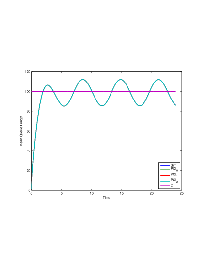
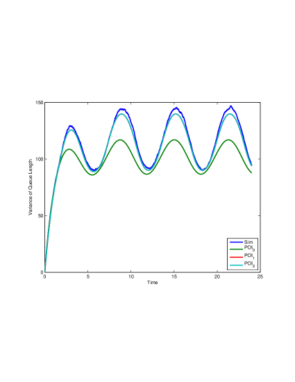
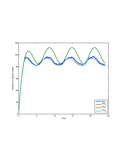
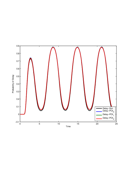
Figure 5.1: $\lambda(t)=100+20\cdot\sin(t)$,  $\mu=1$, $\beta=.75$, $c=100$, $q(0)=1$ (Left).
$\lambda(t)=100+20\cdot\sin(t)$,  $\mu=1$, $\beta=1.25$, $c=100$, $q(0)=1$ (Right).

On the top left of Figure 5.2, we plot the mean of the queueing model with the parameters give in the caption of Figure 5.2. This type of queueing model represents an system where customers are equally patient when compared to the mean service time. In fact, this is equivalent to an infinite server queue. We see that the zeroth and first order approximations are quite good at estimating the mean behavior of the queueing model. On the middle left, of Figure 5.1 we plot the variance and we see that the zeroth and first order approximations are quite accurate, however, unlike Figure 5.1 the zeroth order approximation is as accurate as the first order approximation since the mean is equal to the variance as the Poisson distribution suggests. Lastly on the bottom left of Figure 5.2 we plot the probability of delay of the queueing model and we see that both the zeroth order and the first order are very accurate at estimating its behavior. On the right of Figure 5.2, we have the Erlang-loss model where customers are turned away if too many customers are in the queue. On the right of Figure 5.2, we also see similar behavior for the mean, variance, and probability of delay to the left side for a different set of parameters, which are at the bottom of the caption in Figure 5.2. The zeroth and first order approximations are accurate at estimating the mean, variance, and probability of delay, except for the variance where the first order is much better at estimating its dynamics. Our approximations of the Erlang-loss model indicate that we are able to estimate a variety of queueing and service system models with nonstationary and state dependent rates.

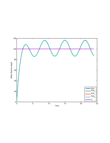
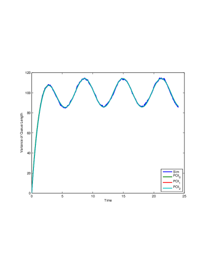
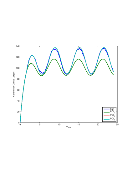
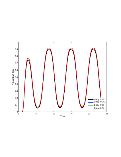
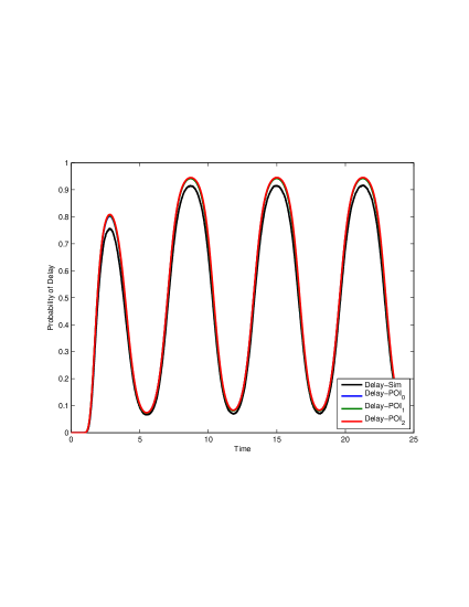
Figure 5.2: $\lambda(t)=100+20\cdot\sin(t)$,  $\mu=1$, $\beta=1$, $c=100$, $q(0)=1$ (Left)
$\lambda(t)=100+20\cdot\sin(t)$,  $\mu=1$, $\beta=.8$, $c=100$, $q(0)=1$, $k=50$ (Right) .

6 Conclusion and Final Remarks

In this paper, we have demonstrated that we can approximate a variety of Markovian birth death processes with nonstationary and state dependent rates. We have used a spectral approach that expands the transition probabilities with the Poisson-Charlier polynomials, which are orthgonal to the Poisson distribution. We have also proven that as we add more terms to the truncated expansion, our approximations converge to the true stochastic process. We gave explicit error bounds on the convergence rate not only for the transition probabilities, but also for the moments of the birth-death process.

There are many new problems that emerge from our work. One obvious, but non-trivial extension to our results that we intend to pursue is the multidimensional setting, where many individual birth-death processes interact with one another in a more complex network. This would involve the multi-dimensional analogue of the Poisson-Charlier polynomials. In the context of operations research and queueing theory problems, this extension would not only provide new approximations for Jackson networks, but also it would allow us to approximate some non-Markovian queueing networks that can be modeled with phase type distributions. Moreover, if we were also able to prove error bounds for our approximations, it would give insight into how close some non-Markovian systems are to the Poisson reference distribution and what parameters affect this closeness.

Appendix A Appendix

A.1 Brief Review of Poisson Distribution and Properties

It is important to know how close our distribution is to the Poisson distribution. The Chen Stein method can help in our understanding of how close our queueing process is to the Poisson distribution.

Theorem A.1 (Chen-Stein).

Let Q be a random variable with values in $\mathbb{N}$. Then, Q has the Poisson distribution with mean rate $q$ if and only if, for every bounded function $f:\mathbb{N}\to\mathbb{N}$,

$$\mathbb{E}\left[Q\cdot f(Q)\right]=q\cdot\mathbb{E}\left[f(Q+1)\right]$$ (A.1)

Proof.

See [18]. ∎

Another important quantity in our calculations for the explicit approximations that are to follow is the incomplete gamma function.

Lemma A.2.

$$\Gamma(c,x)=\sum^{\infty}_{m=c+1}e^{-x}\cdot\frac{x^{m}}{m!}=\frac{1}{\Gamma(c)}\int^{x}_{0}e^{-y}y^{c-1}dy$$

$$\overline{\Gamma}(c,x)=\sum^{c}_{m=0}e^{-x}\cdot\frac{x^{m}}{m!}=\frac{1}{\Gamma(c)}\int^{\infty}_{x}e^{-y}y^{c-1}dy.$$

Proof.

See [7]. ∎

Proposition A.3.

If Q is a Poisson random variable with rate $q>0$, then we have the following expression for the central moments of $Q$

$$E\left[(Q-q)^{m+1}\right]=q\cdot\sum{m\choose j}\cdot E\left[(Q-q)^{j}\right],\quad\mathrm{for}\ \mathrm{all}\ n\in\mathbb{N}$$ (A.2)

Proof.

$$E\left[(Q-q)^{m+1}\right] = \sum^{\infty}_{k=0}(k-q)^{m+1}\cdot e^{-q}\cdot\frac{q^{k}}{k!}$$ (A.3)

$$= e^{-q}\cdot\sum^{\infty}_{k=0}(k-q)^{m+1}\cdot\frac{q^{k}}{k!}$$ (A.4)

$$= e^{-q}\cdot\left(\sum^{\infty}_{k=1}(k-q)^{m}\cdot\frac{q^{k}}{(k-1)!}-q\cdot\sum^{\infty}_{k=0}(k-q)^{m}\cdot\frac{q^{k}}{k!}\right)$$ (A.5)

$$= e^{-q}\cdot q\cdot\sum^{\infty}_{k=0}\left((k+1-q)^{m}-(k-q)^{m}\right)\cdot\frac{q^{k}}{k!}$$ (A.6)

$$= e^{-q}\cdot q\cdot\sum^{\infty}_{k=0}\left(\sum^{m-1}_{j=0}{m\choose j}\cdot(k-q)^{j}\right)\cdot\frac{q^{k}}{k!}$$ (A.7)

$$= e^{-q}\cdot q\cdot\sum^{m-1}_{j=0}{m\choose j}\left(\sum^{\infty}_{k=0}(k-q)^{j}\cdot\frac{q^{k}}{k!}\right)$$ (A.8)

$$= q\cdot\sum^{m-1}_{j=0}{m\choose j}E\left[(Q-q)^{j}\right]$$ (A.9)

∎

A.1.1 Touchard Polynomials and Relation to Poisson Moments

Lemma A.4.

The moments of Poisson random variables have the following expressions in terms of Touchard polynomials $T_{k}$

$$E[Q^{k}] = \sum^{\infty}_{m=0}m^{k}\cdot e^{-q}\cdot\frac{q^{m}}{m!}=T_{k}.$$

In fact the first six Touchard polynomials have the following form

$$T_{1} = q,\quad T_{2}=q^{2}+q,\quad T_{3}=q^{3}+3\cdot q^{2}+q,\quad T_{4}=q^{4}+6\cdot q^{3}+7\cdot q^{2}+q$$

$$T_{5} = q^{5}+10\cdot q^{4}+25\cdot q^{3}+15\cdot q^{2}+q,\quad T_{6}=q^{6}+10\cdot q^{5}+25\cdot q^{4}+15\cdot q^{3}+q^{2}+q.$$

Proof.

This follows from the definintion of the Touchard polynomials. See for example [18]. ∎

Moreover, the Touchard polynomials are also defined by the following expression

$$T_{m}(q) = \sum^{m}_{j=1}S(n,j)\cdot q^{j}=\sum^{m}_{j=1}\left\{\begin{matrix}n\\ j\end{matrix}\right\}q^{j}$$

where S(n,j) is a Stirling number of the second knd the measures the number of partitions of a set that has $n$ elements and is to be separated into $j$ disjoint non-empty subsets.

A.2 Poisson-Charlier Polynomials

In this section, we describe how to use Poisson-Charlier polynomials in conjuction with the functional forward equations in order to construct approximations for our nonstationary queueing processes. The Poisson-Charlier polynomials are an orthogonal polynomial sequence with respect to the Poisson distribution with rate $a$ i.e

$$\omega(x)=e^{-a}\frac{a^{x}}{x!}\quad\quad x=0,1,2,.....$$ (A.10)

As a result, the Poisson-Charlier polynomials solve the following recurrence relation

$$C_{n+1}^{a}(x)=(x-n-a)\cdot C_{n}^{a}(x)-n\cdot\alpha\cdot C_{n-1}^{a}(x).$$ (A.11)

The first four unnormalized Poisson-Charlier polynomials are defined as

$$C_{0}^{a}(x) = 1$$ (A.12)

$$C_{1}^{a}(x) = x-a$$ (A.13)

$$C_{2}^{a}(x) = x^{2}-2\cdot x\cdot a+a^{2}-x$$ (A.14)

$$C_{3}^{a}(x) = x^{3}-3\cdot(a+1)\cdot x^{2}+(3\cdot a^{2}+3\cdot a+2)\cdot x-a^{3}.$$ (A.15)

Now suppose that we have a function f(x), which is defined on the integers and satifies the inequality

$$\sum^{\infty}_{x=0}f^{2}(x)\cdot\omega(a,x)<\infty,\quad\mathrm{for}\ \mathrm{some}\ a>0.$$ (A.16)

Then we have the following expansion in terms of Poisson-Charlier polynomials in the Hilbert space $l^{2}(\mathbb{N},\omega(a,x))$.

Proposition A.5.

Any function f(x) $\in l^{2}(\mathbb{N},\omega(a,x))$ can be expanded into a Poisson-Charlier series i.e.

$$f(x)=\sum^{\infty}_{x=0}c_{j}\cdot C_{j}^{a}(x)$$ (A.17)

where $c_{j}=\sum^{\infty}_{x=0}f(x)C_{j}^{a}(x)\omega(a,x)$.

Proof.

See [17]. ∎

Remark.

This expansion can also be extended to the case where the independent variable of the function f(k) is a stochastic process and also depends on time itself.

Lemma A.6.

$$\sum^{\infty}_{x=0}\omega(a,x)\cdot C_{j}^{a}(x)=E[C_{j}^{a}(x)]=0\quad\mathrm{for}\ \mathrm{all}\ j\geq 1.$$ (A.18)

Proof.

This follows from the orthogonality of the Poisson-Charlier polynomials with constants, which is the zeroth order term. ∎

A.3 Extension: Erlang Loss Queue ($M_{t}/M_{t}/C_{t}/K_{t}+M_{t}$)

$$\raisebox{0.9pt}{$\stackrel{{\scriptstyle\bullet}}{{E}}$}\left[f(Q)\right] = \lambda\cdot E\left[\left(f(Q+1)-f(Q)\right)\cdot\{Q<c+k\}\right]$$ (A.19)

$$+\mu\cdot E\left[\left(Q\wedge c\right)\cdot\left(f(Q-1)-f(Q)\right)\right]$$

$$+\beta\cdot E\left[\left(Q-c\right)^{+}\cdot\left(f(Q-1)-f(Q)\right)\right],$$

for all integrable functions $f$ and $k(t)$ represents the number of waiting spaces in the loss queue.

For the special cases of the mean and variance we have that

$$\raisebox{0.9pt}{$\stackrel{{\scriptstyle\bullet}}{{E}}$}[Q] = \lambda\cdot E[\{Q<c+k\}]-\mu\cdot E[Q\wedge c]-\beta\cdot E[(Q-c)^{+}]$$ (A.20)

$$\raisebox{0.9pt}{$\stackrel{{\scriptstyle\bullet}}{{\mathrm{Var}}}$}[Q] = \lambda\cdot E[\{Q<c+k\}]+\mu\cdot E[Q\wedge c]+\beta\cdot E[(Q-c)^{+}]$$ (A.21)

$$+2\left(\lambda\cdot\mathrm{Cov}[Q,\{Q<c+k\}]-\mu\cdot\mathrm{Cov}[Q,Q\wedge c]-\beta\cdot\mathrm{Cov}[Q,(Q-c)^{+}]\right).$$

Theorem A.7.

Under the zeroth order Poisson-Charlier approximation we have the following rate function values for the Erlang loss queueing model

$$E[(Q-c)^{+}] = a_{0}\cdot\left[q\cdot\Gamma(q,c-1)-c\cdot\Gamma(q,c)\right]$$ (A.22)

$$E[Q\wedge c] = a_{0}\cdot q-a_{0}\cdot\left[q\cdot\Gamma(q,c-1)-c\cdot\Gamma(q,c)\right]$$ (A.23)

$$E[\{Q<c+k\}] = a_{0}\cdot\overline{\Gamma}(q,c+k)$$ (A.24)

Furthermore, under the first order Poisson-Charlier approximation we have the following rate function values for the Erlang-loss queueing model

$$E[(Q-c)^{+}] = a_{0}\cdot\left[q\cdot\Gamma(q,c-1)-c\cdot\Gamma(q,c)\right]$$

$$+a_{1}\cdot\left[q^{2}\cdot\Gamma(q,c-2)+q\cdot\Gamma(q,c-1)-q^{2}\cdot\Gamma(q,c)\right]$$

$$E[Q\wedge c] = (a_{0}+a_{1})\cdot q-a_{0}\cdot\left[q\cdot\Gamma(q,c-1)-c\cdot\Gamma(q,c)\right]$$

$$-a_{1}\cdot\left[q^{2}\cdot\Gamma(q,c-2)+q\cdot\Gamma(q,c-1)-q^{2}\cdot\Gamma(q,c)\right]$$

$$E[\{Q<c+k\}] = a_{0}\cdot\overline{\Gamma}(q,c+k)+a_{1}\cdot\left(q-q\cdot\Gamma(q,c+k-1)-q\cdot\Gamma(q,c+k)\right)$$

$$E[Q\cdot(Q-c)^{+}] = a_{0}\cdot\left(q^{2}\cdot\Gamma(q,c-2)-q\cdot(c-1)\cdot\Gamma(q,c-1)\right)$$

$$+a_{1}\cdot q\cdot\left(q\cdot\Gamma(q,c-2)-c\cdot\Gamma(q,c-1)\right)$$

$$-a_{1}\cdot q\cdot\left(q^{2}\cdot\Gamma(q,c-2)-q\cdot(c-1)\cdot\Gamma(q,c-1)\right)$$

$$E[Q\cdot(Q\wedge c)] = a_{0}\cdot(q^{2}+q)+a_{1}\cdot(2q^{2}+q)-E[Q\cdot(Q-c)^{+}]$$

$$-a_{1}\cdot\left[q^{2}\cdot\Gamma(q,c-2)+q\cdot\Gamma(q,c-1)-q^{2}\cdot\Gamma(q,c)\right]$$

$$E[Q\cdot\{Q<c+k\}] = a_{0}\cdot q\cdot\overline{\Gamma}(q,c+k-1)$$

$$+a_{1}\cdot\left(q^{2}\cdot\overline{\Gamma}(q,z-2)+q\cdot\overline{\Gamma}(q,z-1)-q^{2}\cdot\overline{\Gamma}(q,z-1)\right)$$

A.4 Derivations for Birth-Death Process Rate Functions

Now that we have a good understanding of the Poisson distribution, we are ready to use the properties of the Poisson distirbution to calculate the rate functions that appear in the functional forward equations. The derivation of the expectation and covariance terms that arise from the functional forward equations is an integral part of our method and approximations for birth-death processes. We first start with the zeroth order approximation terms, which assumes the birth-death process has a Poisson distribution.

A.4.1 Zeroth Order Terms

In this section, we will calcuate all of the terms that are needed to derive our zeroth order approximation for the mean and variance of our Markov process models. The first term that we calculate for our explicit approximations is the moments of the Markov process with respect to the Poisson distribution. Since they are intimately related to the Touchard polynomials, the calculation is quite simple.

$$E_{0}[Q^{k}] = \sum^{\infty}_{m=0}m^{k}\cdot\mathbb{P}_{0}(Q=m)$$ (A.25)

$$= \sum^{\infty}_{m=1}m^{k}\cdot e^{-q}\frac{q^{m}}{m!}\left(\sum^{N}_{j=0}a_{j}\cdot C_{j}(q,m)\right)$$ (A.26)

$$= \sum^{\infty}_{m=1}m^{k}\cdot e^{-q}\frac{q^{m}}{m!}\left(a_{0}\cdot C_{0}(q,m)\right)$$ (A.27)

$$= a_{0}\cdot T_{k}$$ (A.28)

The next term is used for the Erlang loss model and is used to approximate the effective arrival rate when blocking occurs. This is also quite simple since it is intimately related to the incomplete gamma function.

$$E_{0}[\{Q<z\}] = a_{0}\cdot(1-\mathbb{P}(Q\geq z))$$ (A.29)

$$= a_{0}\cdot\overline{\Gamma}(q,z)$$ (A.30)

The next term is also related to the Erlang loss system and is needed to approximate the variance or second moment of the Erlang loss model. This term has no interpretation like the previous two, however, using the Chen-Stein identity for the Poisson distribution, it is also quite simple to calculate the expectation.

$$E[Q\cdot\{Q>z\}] = q\cdot E[\{Q+1\geq z\}]$$ (A.31)

$$= q\cdot E[\{Q\geq z-1\}]$$ (A.32)

$$= q\cdot\Gamma(q,z-1)$$ (A.33)

The next term is also used in the approximation for the second moment and variance and we also use the Chen-Stein twice identity to calculate its expectation.

$$E_{0}[Q^{2}\cdot\{Q<z\}] = E_{0}[Q^{2}]-E_{0}[Q^{2}\cdot\{Q\geq z\}]$$ (A.34)

$$= a_{0}\cdot(q^{2}+q)-\sum^{\infty}_{m=z}m^{2}\cdot\mathbb{P}_{0}(Q=m)$$ (A.35)

$$= a_{0}\cdot q-\sum^{\infty}_{m=z}m^{2}\cdot e^{-q}\frac{q^{m}}{m!}$$ (A.36)

$$= a_{0}\cdot\left(q^{2}+q-q^{2}\cdot\Gamma(q,z-2)-q\cdot\Gamma(q,z-1)\right)$$ (A.37)

$$= a_{0}\cdot\left(q^{2}\cdot\overline{\Gamma}(q,z-2)+q\cdot\overline{\Gamma}(q,z-1)\right)$$ (A.38)

The next term also uses the Chen-Stein identity, but three times to calculate its expectation.

$$E_{0}[Q^{3}\cdot\{Q<z\}] = E_{0}[Q^{3}]-E_{0}[Q^{3}\cdot\{Q\geq z\}]$$ (A.39)

$$= a_{0}\cdot\left(q^{3}+3\cdot q^{2}+q-\sum^{\infty}_{m=z}m^{3}\cdot\mathbb{P}_{0}(Q=m)\right)$$ (A.40)

$$= a_{0}\cdot\left(q^{3}+3\cdot q^{2}+q-\sum^{\infty}_{m=z}m^{3}\cdot e^{-q}\frac{q^{m}}{m!}\right)$$ (A.41)

$$= a_{0}\cdot\left(q^{3}\cdot\overline{\Gamma}(q,z-3)+3\cdot q\cdot\overline{\Gamma}(q,z-2)+q\cdot\overline{\Gamma}(q,z-1)\right)$$ (A.42)

The next term is for the expected number of customers that are currently waiting for service. This is calculated explicitly using the incomplete gamma function and the Chen-Stein identity.

$$E_{0}[(Q-c)^{+}] = a_{0}\cdot\left(\sum^{\infty}_{k=c+1}(k-c)\cdot e^{-q}\frac{q^{k}}{k!}\right)$$

$$= a_{0}\cdot\left(\sum^{\infty}_{k=c+1}k\cdot e^{-q}\frac{q^{k}}{k!}-\sum^{\infty}_{k=c+1}c\cdot e^{-q}\frac{q^{k}}{k!}\right)$$

$$= a_{0}\cdot\left(\sum^{\infty}_{k=c+1}q\cdot e^{-q}\frac{q^{k-1}}{(k-1)!}-\sum^{\infty}_{k=c+1}c\cdot e^{-q}\frac{q^{k}}{k!}\right)$$

$$= a_{0}\cdot\left(\sum^{\infty}_{k=c}q\cdot e^{-q}\frac{q^{k}}{k!}-\sum^{\infty}_{k=c+1}c\cdot e^{-q}\frac{q^{k}}{k!}\right)$$

$$= a_{0}\cdot\left(q\cdot\Gamma(q,c-1)-c\cdot\Gamma(q,c)\right)$$

The next term is the expected number of customers that are currently being served by an agent. This is is calculated explicitly using the following relation between the maximum and minimum and the previous results

$$(Q\wedge c)=Q-(Q-c)^{+}.$$ (A.43)

$$E_{0}[(Q\wedge c)] = E_{0}[Q]-E_{0}[(Q-c)^{+}]$$

$$= a_{0}\cdot\left(q-q\cdot\Gamma(q,c-1)+c\cdot\Gamma(q,c)\right)$$

For the next term we use the Chen-Stein identity again to easily compute the expectation.

$$E_{0}[Q\cdot(Q-c)^{+}] = a_{0}\cdot\left(\sum^{\infty}_{k=c+1}(k^{2}-c\cdot k)\cdot e^{-q}\frac{q^{k}}{k!}\right)$$

$$= a_{0}\cdot\left(\sum^{\infty}_{k=c+1}k^{2}\cdot e^{-q}\frac{q^{k}}{k!}-\sum^{\infty}_{k=c+1}k\cdot c\cdot e^{-q}\frac{q^{k}}{k!}\right)$$

$$= a_{0}\cdot\left(\sum^{\infty}_{k=c+1}k\cdot q\cdot e^{-q}\frac{q^{k-1}}{(k-1)!}-\sum^{\infty}_{k=c+1}q\cdot c\cdot e^{-q}\frac{q^{k-1}}{(k-1)!}\right)$$

$$= a_{0}\cdot\left(\sum^{\infty}_{k=c}q^{2}\cdot(k-1)\cdot e^{-q}\frac{q^{k-2}}{(k-1)!}+\sum^{\infty}_{k=c+1}q\cdot e^{-q}\frac{q^{k-1}}{(k-1)!}-\sum^{\infty}_{k=c}q\cdot c\cdot e^{-q}\frac{q^{k}}{k!}\right)$$

$$= a_{0}\cdot\left(q^{2}\cdot\Gamma(q,c-2)-q\cdot(c-1)\cdot\Gamma(q,c-1)\right)$$

This term is also computed using Equation A.43 and previously calculated terms.

$$E_{0}[Q\cdot(Q\wedge c)] = E_{0}\left[Q^{2}\right]-E_{0}[Q\cdot(Q-c)^{+}]$$

$$= a_{0}\cdot\left(q^{2}+q-q^{2}\cdot\Gamma(q,c-2)+q\cdot(c-1)\cdot\Gamma(q,c-1)\right)$$

Finally, the following covariance terms are also calculated using the previous terms.

$$\mathrm{Cov}_{0}[Q,(Q-c)^{+}] = \left(E_{0}[Q\cdot(Q-c)^{+}]-E_{0}[Q]\cdot E_{0}[(Q-c)^{+}]\right)$$

$$= a_{0}\cdot\left(q^{2}\cdot\Gamma(q,c-2)-q\cdot(c-1)\cdot\Gamma(q,c-1)\right)$$

$$- a_{0}\cdot q\cdot a_{0}\cdot\left(q\cdot\Gamma(q,c-1)-c\cdot\Gamma(q,c)\right)$$

$$= a_{0}\cdot\left(q^{2}\cdot\Gamma(q,c-2)-q\cdot(c-1)\cdot\Gamma(q,c-1)\right)$$

$$- a_{0}^{2}\cdot q\cdot\left(q\cdot\Gamma(q,c-1)-c\cdot\Gamma(q,c)\right)$$

$$\mathrm{Cov}_{0}[Q,(Q\wedge c)] = \left(E_{0}[Q\cdot(Q\wedge c)]-E_{0}[Q]\cdot E_{0}[(Q\wedge c)]\right)$$

$$= a_{0}\cdot q-a_{0}\cdot\left(q^{2}\cdot\Gamma(q,c-2)-q\cdot(c-1)\cdot\Gamma(q,c-1)\right)$$

$$+ a_{0}\cdot q\cdot a_{0}\cdot\left(q\cdot\Gamma(q,c-1)-c\cdot\Gamma(q,c)\right)$$

$$= a_{0}\cdot q-a_{0}\cdot\left(q^{2}\cdot\Gamma(q,c-2)-q\cdot(c-1)\cdot\Gamma(q,c-1)\right)$$

$$+ a_{0}^{2}\cdot q\cdot\left(q\cdot\Gamma(q,c-1)-c\cdot\Gamma(q,c)\right)$$

A.4.2 First Order Correction Terms

Now we extend our approximations to the first order correction to the Poisson distribution where all functions are multiplied by the term $a_{1}\cdot(Q-q)$ to incorporate the first Poisson Charlier polynomial. Like in the zeroth order case, many of the terms use the Chen-Stein identity and Equation A.43.

$$E_{1}[Q^{k}] = \sum^{\infty}_{k=0}m^{k}\cdot\mathbb{P}_{1}(Q=m)$$

$$= \sum^{\infty}_{m=1}m^{k}\cdot e^{-q}\frac{q^{m}}{m!}\left(\sum^{1}_{j=0}a_{j}\cdot C_{j}(q,m)\right)$$

$$= \sum^{\infty}_{m=1}m^{k}\cdot e^{-q}\frac{q^{m}}{m!}\left(a_{0}\cdot C_{0}(q,m)+a_{1}\cdot C_{1}(q,m)\right)$$

$$= a_{1}\cdot(T_{k+1}-q\cdot T_{k})$$

$$E_{1}[\{Q<z\}] = a_{1}\cdot E[Q\cdot\{Q<z\}]-a_{1}\cdot q\cdot E[\{Q<z\}]$$

$$= a_{1}\cdot\left(q-q\cdot\Gamma(q,z-1)-q\cdot\Gamma(q,z)\right)$$

$$E_{1}[Q\cdot\{Q<z\}] = a_{1}\cdot\left(E[Q^{2}\cdot\{Q<z\}]-q\cdot E[Q\cdot\{Q<z\}]\right)$$

$$= a_{1}\cdot\left(E[Q^{2}\cdot\{Q<z\}]-q\cdot E[Q\cdot\{Q\geq z\}]\right)$$

$$= a_{1}\cdot\left(q^{2}\cdot\overline{\Gamma}(q,z-2)+q\cdot\overline{\Gamma}(q,z-1)-q^{2}\cdot\overline{\Gamma}(q,z-1)\right)$$

$$E_{1}[Q^{2}\cdot\{Q<z\}] = a_{1}\cdot\left(E[Q^{3}\cdot\{Q<z\}]-q\cdot E[Q^{2}\cdot\{Q<z\}]\right)$$

$$= a_{1}\cdot\left(q^{3}\cdot\overline{\Gamma}(q,z-3)+3\cdot q\cdot\overline{\Gamma}(q,z-2)+q\cdot\overline{\Gamma}(q,z-1)\right)$$

$$- a_{1}\cdot\left(q^{2}\cdot\overline{\Gamma}(q,z-2)-q\cdot\overline{\Gamma}(q,z-1)\right)$$

$$E_{1}[(Q-c)^{+}] = a_{1}\cdot E[Q\cdot(Q-c)^{+}]-q\cdot E[(Q-c)^{+}]$$

$$= a_{1}\cdot\left(q^{2}\cdot\Gamma(q,c-2)-q\cdot(c-1)\cdot\Gamma(q,c-1)\right)-q\cdot\left(q\cdot\Gamma(q,c-1)-c\cdot\Gamma(q,c)\right)$$

$$E_{1}[Q\cdot(Q-c)^{+}] = a_{1}\cdot E[Q^{2}\cdot(Q-c)^{+}]-q\cdot E[Q\cdot(Q-c)^{+}]$$

$$= a_{1}\cdot q\cdot E[(Q+1)\cdot(Q+1-c)^{+}]-q\cdot E[Q\cdot(Q-c)^{+}]$$

$$= a_{1}\cdot q\cdot E[Q\cdot(Q+1-c)^{+}]+a_{1}\cdot q\cdot E[(Q+1-c)^{+}]-q\cdot E[Q\cdot(Q-c)^{+}]$$

$$= a_{1}\cdot q\cdot\left(q^{2}\cdot\Gamma(q,c-3)-q\cdot(c-1)\cdot\Gamma(q,c-2)\right)$$

$$+a_{1}\cdot q\cdot\left(q\cdot\Gamma(q,c-2)-c\cdot\Gamma(q,c-1)\right)$$

$$-a_{1}\cdot q\cdot\left(q^{2}\cdot\Gamma(q,c-2)-q\cdot(c-1)\cdot\Gamma(q,c-1)\right)$$

$$E_{1}[Q\cdot(Q\wedge c)] = E_{1}\left[Q^{2}\right]-E_{1}[Q\cdot(Q-c)^{+}]$$

$$= q^{3}+3\cdot q^{2}+q-q^{2}-q-q^{2}\cdot\Gamma(q,c-2)-q\cdot\Gamma(q,c-1)+q^{2}\cdot\Gamma(q,c)$$

$$= 2\cdot q^{2}+q-q^{2}\cdot\Gamma(q,c-2)-q\cdot\Gamma(q,c-1)+q^{2}\cdot\Gamma(q,c)$$

Thus, the first order approximation of the covariance terms have the following expressions in terms of previously calculated ones:

$$\mathrm{Cov}[Q,(Q-c)^{+}] = \left(E_{0}[Q\cdot(Q-c)^{+}]+E_{1}[Q\cdot(Q-c)^{+}]\right)$$

$$-\left(E_{0}[Q]+E_{1}[Q]\right)\cdot\left(E_{0}[(Q-c)^{+}]+E_{1}[(Q-c)^{+}]\right)$$

$$\mathrm{Cov}_{1}[Q,(Q\wedge c)] = \mathrm{Var}[Q]-\mathrm{Cov}[Q,(Q-c)^{+}]$$

$$\mathrm{Cov}[Q,\{Q<z\}] = \left(E_{0}[Q\cdot\{Q<z\}]+E_{1}[Q\cdot\{Q<z\}]\right)$$

$$-\left(E_{0}[Q]+E_{1}[Q]\right)\cdot\left(E_{0}[\{Q<z\}]+E_{1}[\{Q<z\}]\right)$$

We stop here at the zeroth and first order approximations, however, we can also derive similar expressions of the rate functions for higher moments and higher orders of the approximation using the same methodolgy and Chen-Stein identity if they are needed in other applications or settings.

References

• Brémaud [1999] P. Brémaud. Markov Chains: Gibbs Fields, Monte Carlo Simulation, and Queues. Number 31 in Texts in Applied Mathematics. Springer, New York, 1999.
• Clark [1981] G. M. Clark. Use of Polya distributions in approximate solutions to nonstationary M/M/s queues. Communications of the ACM, 24(4):206–217, 1981.
• Deuflhard et al. [2008] P. Deuflhard, W. Huisinga, T. Jahnke, and M. Wulkow. Adaptive discrete galerkin methods applied to the chemical master equation. SIAM Journal on Scientific Computing, 30(6):2990–3011, 2008.
• Engblom [2012] S. Engblom. On the stability of stochastic jump kinetics. Technical Report 2012-005, Dept of Information Technology, Uppsala University, 2012. Available at http://arxiv.org/abs/1202.3892.
• S. Engblom [2009] S. Engblom. Spectral approximation of solutions to the chemical master equation. J. Comput. Appl. Math., 229(1):208–221, 2009. doi:10.1016/j.cam.2008.10.029.
• S. Engblom [2009] S. Engblom. Galerkin spectral method applied to the chemical master equation. Commun. Comput. Phys., 5(5):871–896, 2009.
• Janssen et al. [2008] A. Janssen, J. Van Leeuwaarden, B. Zwart, et al. Gaussian expansions and bounds for the Poisson distribution applied to the erlang b formula. Advances in Applied Probability, 40(1):122–143, 2008.
• Koekoek and Swarttouw [1998] R. Koekoek and R. F. Swarttouw. The Askey-scheme of hypergeometric orthogonal polynomials and its $q$-analogue. Technical Report 98-17, Delft University of Technology, Faculty of Information Technology and Systems, Department of Technical Mathematics and Informatics, 1998. Available at http://aw.twi.tudelft.nl/$\sim$koekoek/askey.html.
• Krishnarajah et al. [2005] I. Krishnarajah, A. Cook, G. Marion, and G. Gibson. Novel moment closure approximations in stochastic epidemics. Bulletin of mathematical biology, 67(4):855–873, 2005.
• Krishnarajah et al. [2007] I. Krishnarajah, G. Marion, and G. Gibson. Novel bivariate moment-closure approximations. Mathematical biosciences, 208(2):621–643, 2007.
• Mandelbaum et al. [1998] A. Mandelbaum, W. A. Massey, and M. I. Reiman. Strong approximations for Markovian service networks. Queueing Systems, 30(1-2):149–201, 1998.
• Massey [1985] W. Massey. Asymptotic Analysis of the Time Dependent M/M/1 Queue. Mathematics of Operations Research, 10(10):305–327, 1985.
• Massey and Pender [2011] W. Massey and J. Pender. Skewness Variance Approximation for Dynamic Rate Multi-server Queues with Abandonment. Performance Evaluation Review, 39:74–74, 2011.
• Massey and Pender [2013] W. Massey and J. Pender. Gaussian skewness approximation for dynamic rate multi-server queues with abandonment. Queueing Systems, 75(2):243–277, 2013.
• Massey and Pender [2014] W. Massey and J. Pender. Approximating and Stabilizing Jackson Networks with Abandonment. 2014.
• Meyn and Tweedie [1993] S. P. Meyn and R. L. Tweedie. Stability of Markovian processes iii: Foster-Lyapunov criteria for continuous-time processes. Adv. in Appl. Probab., 25(3):518–548, 1993.
• Ogura [1972] H. Ogura. Orthogonal functionals of the Poisson process. IEEE Transactions on Information Theory, 18(4):473–481, 1972.
• Peccati and Taqqu [2011] G. Peccati and M. S. Taqqu. Wiener Chaos: Moments, Cumulants and Diagrams: A Survey with Computer Implementation, volume 1. Springer, 2011.
• Pender [2014] J. Pender. A Poisson-Charlier Approximation for Nonstationary Queues. Operations Research Letters, 2014.
• J. Pender [2014] J. Pender. Laguerre Polynomial Expansions for Time Varying Multiserver Queues with Abandonment. Available at http://www.columbia.edu/$\sim$jp3404/LSA.html, 2014.
• Rothkopf and Oren [1979] M. H. Rothkopf and S. S. Oren. A Closure approximation for the Nonstationary M/M/s queue. Management Science, 25(6):522–534, 1979.
• Taaffe and Ong [1987] M. R. Taaffe and K. L. Ong. Approximating Nonstationary Ph(t)/M(t)/s/c queueing systems. Annals of Operations Research, 8(1):103–116, 1987.
• Wulkow [1992] M. Wulkow. Adaptive treatment of polyreactions in weighted sequence spaces. IMPACT Comput. Sci. Eng., 4(2):153–193, 1992. doi:10.1016/0899-8248(92)90020-9.
• Wulkow [1996] M. Wulkow. The simulation of molecular weight distributions in polyreaction kinetics by discrete Galerkin methods. Macromol. Theory. Simul., 5(3):393–416, 1996. doi:10.1002/mats.1996.040050303.