Incorporating Near-Infrared Information 
into Semantic Image Segmentation

Abstract

Recent progress in computational photography has shown that we can acquire near-infrared (NIR) information in addition to the normal visible (RGB) band, with only slight modifications to standard digital cameras. Due to the proximity of the NIR band to visible radiation, NIR images share many properties with visible images. However, as a result of the material dependent reflection in the NIR part of the spectrum, such images reveal different characteristics of the scene. We investigate how to effectively exploit these differences to improve performance on the semantic image segmentation task. Based on a state-of-the-art segmentation framework and a novel manually segmented image database (both indoor and outdoor scenes) that contain 4-channel images (RGB+NIR), we study how to best incorporate the specific characteristics of the NIR response. We show that adding NIR leads to improved performance for classes that correspond to a specific type of material in both outdoor and indoor scenes. We also discuss the results with respect to the physical properties of the NIR response.

1 Introduction

In computer vision, semantic image segmentation is the task that assigns a semantic label to every pixel in an image. For example, an outdoor image could be segmented into different regions (i.e.,  groups of pixels) that correspond to the labels $grass$, $sky$, $tree$, and $water$ (see Figure 1 for an example). Semantic segmentation thus necessitates the joint recognition and localization of several classes of interest, that can be both object classes or background classes.

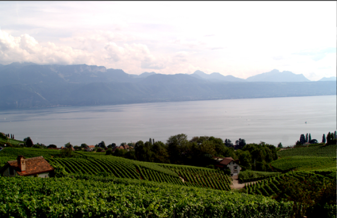
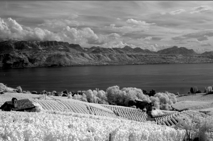
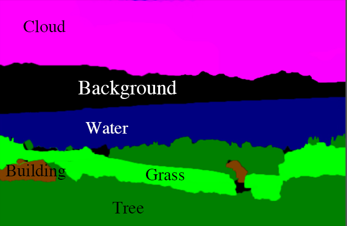
RGB	NIR	Groundtruth segmentation

Figure 1: The semantic segmentation task consists in labeling every pixel of an image as belonging to one of the classes of interest (e.g.,  : $grass$, $sky$, $tree$, $water$) or to the background. Here, we demonstrate that semantic segmentation can be improved with additional near-infrared information.

This task has received a lot of attention over the last decade, and many methods have been proposed to semantically segment RGB images shotton2006 ; verbeek2007 ; schmid2008 ; larlus2010 ; csurka2011 ; koltun2011 . Most proposed models combine two components: (i) a local recognition process that identifies the classes and (ii) a regularization process that groups the pixels into semantic regions, often using contour information. Promising results have been obtained over a broad range of categories and for a large variety of scenes, but the problem is far from being solved. Segmentation algorithms tend to fail in the presence of a cluttered background or distractor objects, as well as when the objects to be segmented are composed of several colors or patterns. Figure 2-a shows instances of the $cup$ class that are difficult to segment. Because of surface color variations, even for classes with a consistent color, such as $vegetation$, relying solely on RGB-based features can be insufficient as the color can drastically vary under different lighting conditions.

All these difficulties challenge both components of the segmentation models. The recognition part that learns an appearance model of categories based solely on RGB values has issues with objects where both the color and the texture significantly vary within the object classes, which is the case for most man-made objects. Concerning the regularization part, object contours can be easily confused with strong edges originating from texture patterns on the object, background clutters or any distracting regions.

One way to overcome these issues is to incorporate additional information within the segmentation process. It was shown for example in Crabb2008 that adding depth information when available (e.g.,  obtained with stereo cameras or using range sensor data) can significantly improve segmentation results. Other methods have considered multi-spectral data to enhance segmentation Blaschke2010 . However, these methods require costly and specific acquisition equipment.

In this paper, we consider additional information that can be obtained from a standard digital camera: the near-infrared part of the spectrum that is captured by consumer camera sensors. We study this near-infrared channel in addition to RGB images in the context of semantic image segmentation. This paper extends the work presented in Salamati2012 by studying a wider range of scene types, and a deeper analysis of the results. We use the same state-of-the-art segmentation framework as Salamati2012 . To evaluate the proposed approach, first we contribute with a dataset that extends the ones of brown2011 ; Salamati2012 with pixel-level annotation of 770 registered RGB and NIR image pairs for 23 semantic classes. In order to discuss the advantages that NIR brings to each class of material, the dataset is split into indoor and outdoor scenes and the performance is reported on each subset separately. The outdoor dataset contains 10 different classes, and the indoor dataset contains 13 classes.

Our second contribution is an in-depth study of the results obtained by our proposed model. We extended a state-of-the-art segmentation framework with different strategies for incorporating the NIR channel that improve over conventional RGB-only segmentation results. This framework is based on a conditional random field (CRF), where we exploit different ways to combine the visible and NIR information in the recognition part and in the regularization part of the model. Based on the segmentation results, the paper fully discusses the accuracy obtained for each class of material, together with success and failure cases, and puts them in perspective with the material characteristics of the NIR radiation. In particular, we show that the overall improvement is due to a large improvement for certain classes whose response in the NIR domain is particularly discriminant.

The rest of this article is organized as follows. Section 2 reviews the relevant literature on NIR imaging while Section 3 discusses different approaches to semantic segmentation. Section 4 describes our semantic image segmentation system. The experimental setup and evaluation procedure are explained in Section 5 and experimental results are exposed and discussed in Section 6 and 7. Section 8 concludes the paper.

2 Near-infrared (NIR)

2.1 NIR properties and their relevance to segmentation

NIR spectra are influenced by the chemical and physical structure of different material classes, which makes NIR suitable for material classification burns2001 . Figure 3 shows that for a given material, regardless of the object color in the visible part (400-700 nm), the reflection in the NIR band (700-1100 nm) remains the same.

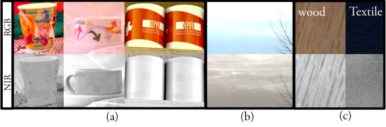
Figure 2: Challenging cases for RGB-only semantic segmentation. In NIR images (a) cups in different colors have the same brightness, (b) haze is transparent, and (c) texture is more intrinsic to the material.

salamati2009 shows that each class of material has an intrinsic behavior in the near-infrared (NIR) part of the spectrum. The material dependency of NIR reflection has been proven to be useful in low-level segmentation salamati2010 and produces segments that correspond to changes of material salamati2010 . Our previous works show that NIR could enhance scene classification salamati2011 and semantic segmentation as well Salamati2012 .

The properties of infrared images Morris2007 have been used by the remote sensing zhou2009 ; walter2004 and military dowdall2005 communities for many years to detect and classify natural and/or man-made objects. However, in this paper we approach semantic image segmentation from a different point of view. Unlike most remote sensing applications that use true hyper-spectral capture with several bands in the NIR part and the IR part of the spectrum, our framework only uses one single channel that integrates all NIR radiation. The single NIR channel can be captured by the standard sensor of any digital camera. Moreover, in remote sensing and military applications, the focus is mostly on aerial photography, forgery, and human detection, while this work tackles semantic segmentation in everyday photography.

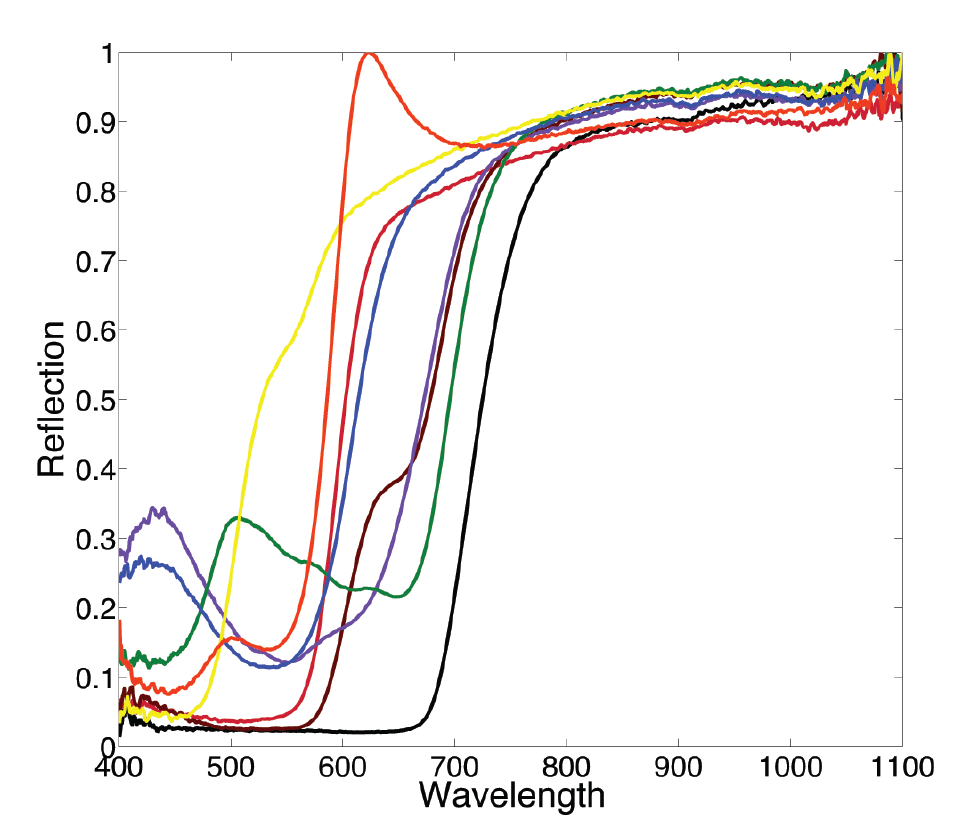
Figure 3: Spectral reflectance of 20 different fabrics. The reflection of these samples is different in the visible part of the spectrum, which for a given camera and lighting condition leads to different color values. However, as these samples belong to the same material, their spectral reflectance in the NIR range is not significantly different.

As already mentioned earlier, state-of-the-art semantic segmentation techniques still encounter some difficulties in both recognizing different classes and detecting the actual boundary of semantic objects. Such shortcomings are mostly due to four reasons : appearance variation, cluttered backgrounds, illumination differences, and hazy atmosphere in outdoor scenes. Learning a color-based appearance model of classes based only on RGB values is very challenging due to the appearance variation of a single object, or the varying lighting conditions. As another situation, the segmentation of $cloud$ and $mountain$ classes often fail in a hazy atmosphere (see Figure 2-b for illustration). Texture has shown to be a powerful cue for semantic segmentation csurka2011 ; nils2009 . However, texture can be confused with color patterns and other immediate surface impurities, as surface reflectance in the visible part of the spectrum that is not intrinsic to the corresponding object material (see Figure 2-c for illustration).

Light in the near-infrared range has physical properties intrinsically different than in the visible range. The intensity values in NIR images are more consistent across a single material and consequently across a given class region. For instance, vegetation is consistently very bright, and sky and water are very absorbent in the NIR band. Furthermore, a large number of colorants and dyes are transparent to NIR. Thus, material-intrinsic texture properties are easier to capture in this part of the spectrum.

Because of all these reasons, NIR is a great complement to the visible information and improves the labeling of the semantic classes that correspond to specific materials or textures. For instance, the class $cup$ is often made of very specific classes of material (porcelain, ceramic or plastic) and regardless of the pattern and color of the object, NIR has a unique response for each of these materials (see Figure 2-a for illustration). Another interesting aspect is the fact that atmospheric haze is transparent to NIR, hence the borders of objects in hazy weather conditions is better defined in NIR images.

2.2 NIR imaging

NIR imaging is used in different areas of science.

NIR spectroscopy (NIRS) is employed for material identification and forgery detection. NIRS is a non-destructive technique used to study the interactions between incident light and material surfaces; it is based on the assumption that surface reflection in the NIR band proves to be critical for detection of different classes of material burns2001 ; whelan2003 . The need for little or no preparation of samples has made it one of the most used techniques for material identification in industry burns2001 .

In remote sensing, multi-spectral images are captured in order to detect, characterize and monitor different regions, such as vegetation and soil. In such applications, region reflection in both the visible and IR parts of the spectrum is required zhou2009 ; walter2004 . It has been shown that both offer valuable information providing bio-signatures for different classes of vegetation and soil properties blackburn2007 .

In both remote sensing and NIR spectroscopy, hyper-spectral data is needed to accurately identify material classes. However, these capturing devices are highly technical and expensive, hence they are of limited usefulness outside laboratory conditions.

The most common sensors in consumer digital cameras, i.e.,  CMOS, is made of silicon and thus is intrinsically sensitive to wavelengths from roughly 350 nm to 1100 nm. The material employed to create the color filter array (CFA) is also transparent to the NIR. Figure 4 shows the transmittance of the CFA filters of a NikonD90 with the hot mirror (NIR-blocking filter that is normally put by manufacturer) removed. Hence, if the NIR-blocking filter is omitted from the camera, the sensor has the capability to capture both NIR and visible bands; no modification of the sensor is required as shown in fredembach2008 .

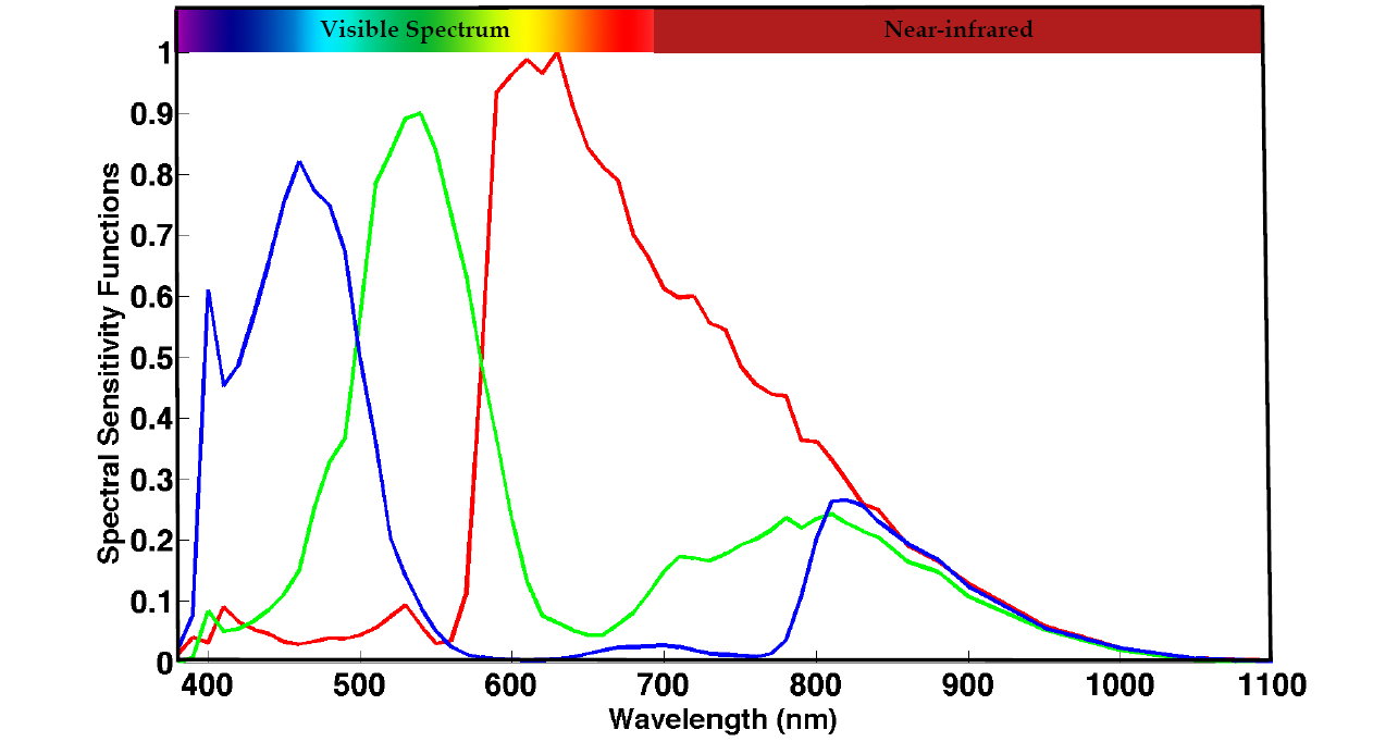
Figure 4: Typical transmittance curves of the RGB filters of the silicon sensor found in the NikonD90 camera.

Currently, two main methods are used to jointly capture the NIR and visible images. The first approach uses two cameras with a beam splitter zhang2008 . In the second approach, a camera with NIR and visible filters is used to sequentially capture two images that are then registered fredembach2008 . As a third method, Kermani et. al.  designed a new color filter array that could be used for demosaicing the “full-spectrum” raw data into a visible and NIR pair kermani2011 . Although all the images we used in our experiments have been acquired with the second approach, any of these acquisition methods can be used with the proposed approach.

Several recent works have used such 4-dimensional images – RGB and NIR channels – for standard computer graphics and computer vision tasks. In image enhancement, we can mention haze removal Schaul2009 , skin enhancement Fredembach2010 , dark-flash photography Krishnan2009 , videoconferencing hppeople , and real-time 3-dimensional depth imaging kinektpeople . In computer vision, the intrinsic properties of material classes in NIR images make this information a relevant choice in image scene classification brown2011 ; salamati2011 or material-based segmentation salamati2010 .

3 Semantic Segmentation

Semantic image segmentation is the computer vision task that consists in partitioning an image into different semantic regions, where each region corresponds to a class. It can be seen as a pixel-level categorization task.

The appearance of the classes of interest are learnt during a training step from images annotated at the pixel-level. Learnt models are based on appearance descriptors that are often based on Gaussian derivative filter outputs or texture descriptors such as SIFT lowe2004 , or based on colors statistics vandeweijer2006 ; clinchant07 . Appearance descriptors are extracted at the pixel-level shotton2006 ; shotton2008 or statistics are extracted at the patch level, on a (multi-scale) grid of patches csurka2011 ; verbeek2007 ; larlus2010 , or at detected interest point locations yang07 . The location of the pixels is sometimes used as a cue as well shotton2006 ; shotton2008 . In general, low-level features are used to build higher-level representations, such as texton forests shotton2008 , bags-of-visual-words (BoVW) larlus2010 ; verbeek2007 , or Fisher vectors csurka2011 ; Hu2012 that are fed into a classifier to predict class labels at pixel level shotton2008 , patch level larlus2010 ; csurka2011 or region level yang07 .

The local appearance models are often combined with a local label consistency component that adds constraints on neighboring pixels shotton2006 ; larlus2010 or within an image region (super-pixel) csurka2011 ; Hu2012 . Sometimes, global consistency also takes into account the whole image shotton2006 ; larlus2010 and/or the context of the object class ladicky2010 . State-of-the-art semantic segmentation methods typically integrate these components into a unified probabilistic framework such as a conditional random field (CRF) verbeek2007 ; kohli2009 ; ladicky2009 ; kohli2010 ; larlus2010 ; Hu2012 , or these components are learnt independently and used at different stages of a sequential pipeline yang07 ; csurka2011 .

In this paper, we consider the former and use a CRF model that combines local appearance predictions with local consistency of labels. Label consistency is enforced by a set of pairwise constraints between neighboring pixels. We used a standard contrast-sensitive Potts model. Note that more complex CRF models were proposed that incorporate object co-occurrences ladicky2010 or object detectors ladicky2010and , use fully connected CRF models koltun2011 , hierarchical associative CRFs ladicky2009 or higher order potentials kohli2009 ; kohli2010 . The aim of our paper is to evaluate the potential advantage of the NIR information in a standard semantic image segmentation model, so we used a very standard CRF model and we do not consider these more complex models. We believe that the conclusions of this paper would extend to these models and that this constitutes potential extensions of the presented framework. Comparing these methods is beyond the score of this paper.

4 Our CRF framework

We represent the label of a pixel $i$ with a random variable $X_{i}$ taking a value from the set of labels $\mathcal{L}=\{l_{1},\dots,l_{n}\}$, $n$ being the number of classes. Let $X$ be the set of random variables representing the labeling of an image and $X=\textbf{x}$ an actual ($i.e.$, possible) labeling. The posterior distribution $P(X=\textbf{x}\mid\textbf{D})$, given the observation D over all possible labeling of a CRF, is a $Gibbs$ distribution and can be written as:

$$P(X=\textbf{x}\mid\textbf{D})=\frac{1}{Z}\exp(\;-\underbrace{\sum_{c\in C}\psi_{c}(\textbf{x}_{c})}_{E(\textbf{x})}\;)$$ (1)

where $\psi_{c}(\textbf{x}_{c})$ are potential functions over the variables $\textbf{x}_{c}=\{x_{i},i\in c\}$ and $Z$ is a normalization factor. In this equation, a clique $c$ defines a set of random variables $X_{c}\subseteq X$ that depend on each other, and $C$ is the set of all cliques. Please note that the observation D represents the actual pixel values in the image. Accordingly, the $Gibbs$ energy is defined as

$$E(\textbf{x})=-\log(P(X=\textbf{x}\mid\textbf{D}))-\log Z$$ (2)

Using these notations, the goal of semantic segmentation is to find the most probable labeling x^∗, which is defined as the maximum a posteriori (MAP) labeling:

$$\textbf{x}^{*}=\textrm{argmax}_{\textbf{x}\in\mathcal{L}^{N}}\,P(X=\textbf{x}\mid\textbf{D})=\textrm{argmin}_{\textbf{x}\in\mathcal{L}^{N}}\,E(\textbf{x})$$

where $N$ is the number of pixels.

In our CRF model, the energy function $E$ is composed of two terms, a unary potential $E_{un}$ and a pairwise potential $E_{pair}$ . The unary term is responsible for the recognition part of the model and the pairwise term encourages neighboring pixels to share the same label. We assign a weight $\lambda$ to $E_{pair}$ that models the trade-off between recognition and spatial regularization. More formally,

$$E(\textbf{x}) =E_{un}(\textbf{x})+\lambda E_{pair}(\textbf{x})$$

$$=\sum_{i\in\nu}\psi_{i}(x_{i})+\lambda\sum_{(i,j)\in\varepsilon}\psi_{i,j}(x_{i},x_{j})$$ (3)

where $\nu$ corresponds to the set of all image pixels and $\varepsilon$ the set of all edges connecting the pixels $i,j\in\nu$. Usually, 4-neighborhood or 8-neighborhood systems are considered. We used the former.

Usually, these models consider unary and pairwise potentials that are built using information extracted from RGB images. In the following, we show how to extend both the unary and the pairwise potential by integrating the NIR channel in the above energy term.

4.1 The unary term

The unary part of the CRF ($E_{un}$) is defined as the negative log likelihood of a label being assigned to pixel $i$. It can be computed from the local appearance model for each class.

$$E_{un}(\textbf{x})=\sum_{i\in\nu}\psi_{i}(x_{i})=\sum_{i\in\nu}-\log(P(X_{i}=\textbf{x}_{i}\mid\textbf{D}))$$

Although the CRF uses pixels, the recognition could be made at several levels. We could describe pixels directly, or work with patches extracted following a regular grid. To build our local appearance model we follow csurka2011 and use patch-level Fisher Vector (FV) representations. FVs Perronnin2010 encode higher order statistics than the visual word counts in the Bag-of-Visual-Words (BoVW) representation csurka2004 . We chose to use FV as they outperform the BoVW (as shown in csurka2011 ), and as they are highly competitive for object classification even with linear classifiers chatfield2011 . However, any similar representation could also have been used for the study.

In a nutshell, our approach is the following: We extract overlapping image patches on a multi-scale grid and describe them with low-level descriptors. The dimension of these features is reduced using principal component analysis (PCA) before building a Gaussian mixture model (GMM) based visual codebook that allows to transform the low-level representation of each patch into a FV (see Perronnin2010 ; csurka2011 for more details). For each class, we train a patch-level linear classifier using strongly labeled training images (i.e.,  segmented images), and the classification score of each patch in a test image is transformed into a probability. The class posterior probabilities at the pixel level are obtained as a weighted average of the patch posteriors, where the weights are given by the distance of the pixel to the center of the patch as in csurka2011 .

Several types of features can be used to describe patches. The most popular descriptors for RGB (=visible) images are color and texture features. Here, we consider the popular SIFT lowe2004 feature to describe the local texture and local color statistics clinchant07 to describe the color. The latter, referred to as $COL$, encodes the mean and standard deviation of the intensity values in each image channel for each cell of a 4x4 grid covering the patch (same cells as in the case of $SIFT$). In our visible-baseline approach, these color statistics are computed on the R,G and B channels, hence we will denote their concatenation by $COL_{rgb}$.

SIFT encodes local texture with a set of histograms of oriented gradients computed on a 4x4 grid covering the patch. In general, it is computed on the patch extracted from the luma channel of the visible RGB image that can be approximated by $L=0,299R+0,587G+0,114B$. It will therefore be denoted by $SIFT_{l}$.

SIFT is sometimes extended by computing histograms of oriented gradients in each color channel and by concatenating the obtained histograms. This descriptor is called multi-spectral SIFT and denoted by $SIFT_{rgb}$.

When an additional NIR channel is considered, we can also extract the corresponding color and SIFT descriptors. We will denote the additional ones by $COL_{n}$ and $SIFT_{n}$, respectively. We can concatenate them with features extracted from the standard RGB image leading to e.g.,  $COL_{rgbn}$ or $SIFT_{rgbn}$.

Due to the high correlation of RGB and NIR channels, brown2011 shows that incorporating NIR information in a de-correlated space improves the performance of image classification. We make use of the same idea, decorrelating the 4-dimensional RGB-NIR color vector by performing Principal Component Analysis (PCA). In this alternative PCA space, we consider $COL_{p1234}$ and $SIFT_{p1234}$ (see brown2011 ; salamati2011 for more details).

In Section 6, we compare and discuss the performance of using each of these descriptors in the unary term of our energy function.

4.2 Pairwise term

The pairwise term $E_{pair}$ of our CRF takes the form of a contrast sensitive Potts model:

$$E_{pair}(\textbf{x}) =\sum_{(i,j)\in\varepsilon}\psi_{i,j}(x_{i},x_{j})$$

$$=\sum_{(i,j)\in\varepsilon}\bar{\delta}_{x_{i},x_{j}}\exp(-\beta\parallel q_{i}-q_{j}\parallel^{2})$$ (4)

where $\bar{\delta}_{x_{i},x_{j}}=1$ if $x_{i}\neq x_{j}$ and $\bar{\delta}_{x_{i},x_{j}}=0$ otherwise. We set $\beta=({2<\parallel q_{i}-q_{j}\parallel^{2}>})^{(-1)}$, as in the work of rother2004 . This potential penalizes disagreeing labels in neighboring pixels, and the penalty is lower where the image intensity changes. In this way, borders between predicted regions are encouraged to follow image edges.

In general, the pixel values $q_{i}$ in the Potts model correspond to the RGB values of pixels. When this is the case we denote the pairwise term by $VIS$, as it corresponds to the visible baseline that uses only the RGB image. However, when NIR information is available, we can use the NIR channel in the pairwise potential. In this case, $q_{i}$ corresponds to the intensity of the pixel in the NIR channel, and the potential will be denoted by $NIR$. Finally, when the Potts model uses the intensity values from the 4 channels ($q_{i}$ is 4 dimensional), the pairwise potential is denoted by $VIS+NIR$.

4.3 Model inference

Given the CRF model defined in Eq (4), we want to find the most probable labeling (x*), i.e.,  the labeling that maximizes the posterior distribution or that minimizes our energy function. This is a NP-hard problem for many practical multi-label computer vision problems and approximation algorithms have to be used. For our model, inference is carried out by the multi-label graph-optimization library of boykov2001 ; boykov2004 ; komogorov2004 , using $\alpha$-expansion. $\alpha$-expansion reduces the multi-label optimization problem to a sequence of binary optimization problems. Given a labeling x, each pixel $i$ makes a binary decision to keep its current label or switch to label $\alpha$ ($\alpha\in\mathcal{L}$).

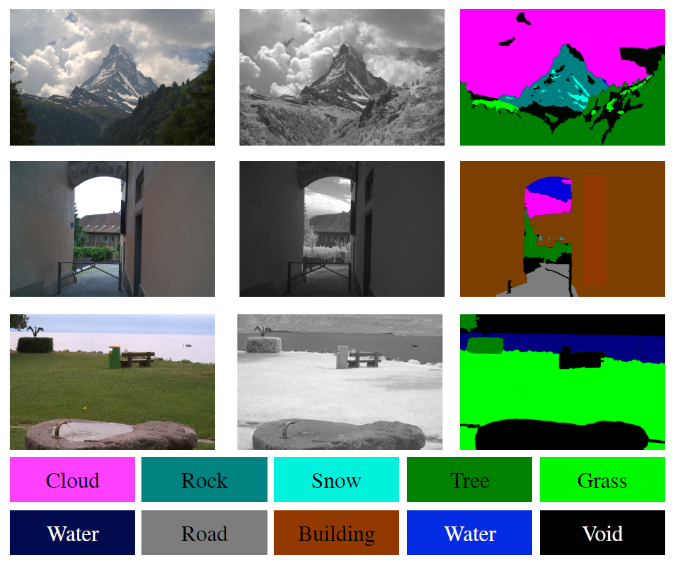
Figure 5: Sample images from our outdoor dataset: RGB (left), NIR (middle), groundtruth pixel-level annotation (right).

5 Datasets and experimental setup

5.1 Proposed datasets

In order to evaluate and better understand the gain of incorporating NIR information in different parts of our CRF model, we labeled a scene segmentation dataset of 770 images with pixel level annotation considering 23 semantic classes. Although this dataset is smaller than the most recent visible only segmentation datasets, it constitutes the very first test-bed for RGB+NIR semantic segmentation, and already allows to conduct a deep study, as shown in our experiments. It is composed of two types of scenes: indoor and outdoor scenes. We conducted separate experiments on both. Examples of 4-channel images for these two datasets and their annotations can be seen in Figure 5 and Figure 6.

The outdoor dataset was built from the 477 RGB and NIR image pairs released by brown2011 . From these images, we discarded 107 images due to mis-registration and ambiguity of classes. The rest of the images were manually labeled at the pixel level, thus yielding pixel segmentation masks. The labels were selected from 10 predefined classes: building (179), cloud (161), grass (159), road (108), rock (80), sky (174), snow (41), soil (78), tree (274), and water (79). We followed the MSRC dataset’s annotation style shotton2006 , i.e.,  each pixel is labeled as belonging to one of the above classes or to a void class. The latter corresponds to pixels whose class is not defined as part of our classes of interest, or that are too ambiguous to be labeled. Similarly to shotton2006 , in this outdoor dataset, we discarded the pixels of the void class from the evaluation.

The indoor dataset consists of 400 images that we specifically gathered in various office environments using sequential capture and registration, as done in brown2011 . The registration between RGB and NIR images was conducted with the algorithm proposed in szeliski2006 . For these images we selected 13 object categories: screen (206), clothing items (184), keyboard (178), cellphone (108), mouse (145), office phone (113), cup (163), bottle (130), potted plant (77), bag (123), office lamp (70), can (59). These objects were manually segmented and annotated at the pixel level, as in the PASCAL VOC Challenge everingham , where all pixels not belonging to the predefined classes are considered as background. Contrary to the void class, the segmentation performance of the predicted background is evaluated.

The background class, however, is rather diverse. Therefore, instead of modeling it explicitly, we first predict only the other classes and then we employ a minimum level of confidence threshold on the predicted classification scores. If the maximum posterior probability is smaller than a single universal threshold (in our case $\mathcal{T}=0.5$), the pixel is labeled as background, otherwise it is labeled with the class label for which the maximum was found. In other words, in our CRF model, $P(X=Background\mid\textbf{D})=\mathcal{T}$.

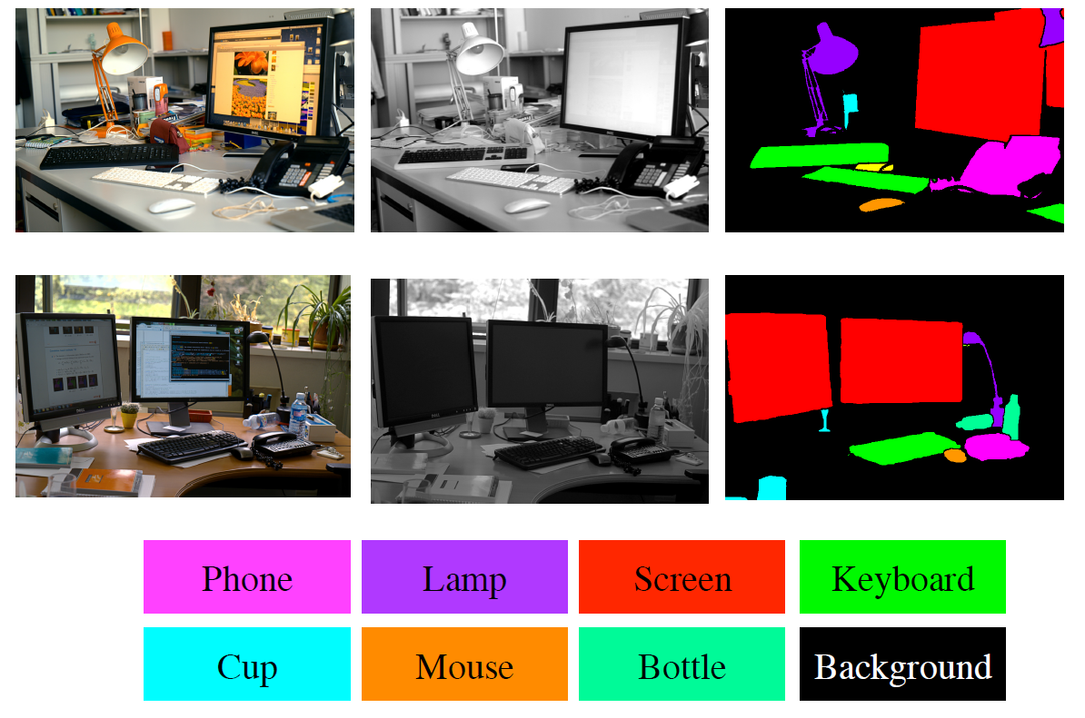
Figure 6: Sample images from our indoor dataset: RGB (left), NIR (middle), ground truth pixel-level annotation (right).

5.2 Experimental details

We extract $32\times 32$ patches on a regular grid (every 10 pixels), at 5 different scales (the first 5 terms of the geometric series with ratio $\sqrt{2}$) in a given channel. Hence the coarsest scale corresponds to re-sizing the patch by a factor of 4 (${\sqrt{2}}^{4}$) and the finest corresponds to the original patch (${\sqrt{2}}^{0}=1$).

Low-level descriptors are computed for each patch. We consider two different descriptors: SIFT descriptors lowe2004 and local color statistics clinchant07 , denoted by $SIFT$ and $COL$ respectively. To compute these features in any of the considered channels (initial channels $R,G,B,N$, luma $L$ or alternative color spaces $P_{1},P_{2},P_{3},P_{4}$), we proceed as follows. A single $SIFT$ is 128-dimensional while $COL$ is 32-dimensional, because we consider the mean and the variance of the color intensity using a 4x4 grid on the patch. Then we concatenate the relevant features, hence $COL_{rgb}$ will be 96 dimensional, $COL_{rgbn}$ will be 128 dimensional, and $SIFT_{rgbn}$ will be 512 dimensional. For a fair comparison, PCA projection is used to reduce all features to 96 dimensions. In the projected space a GMM-based visual codebook of 128 Gaussians is built and used to transform each low-level feature into a Fisher Vector (FV) representation Perronnin2010 . By using the same PCA projection and the same codebook size, the FV representation of all descriptors share the same dimension.

Sparse Logistic Regression (SLR) krishnapuram05 is used for the classification of the patches and the output is a probability obtained from $\frac{1}{1+\exp(-s_{k})}$, where $s_{k},k\in\mathcal{L}$ are the classification scores of the FVs. The class probabilities of each pixel $P(X_{i}=k\mid\textbf{D})$ are then computed as a weighted average of the patch posteriors as described in Section 4.1.

5.3 Evaluation procedure

In all our experiments, we randomly split the dataset into 5 sets of images (5 folds) and define 5 sets of experiments accordingly. For each experiment, one fold is used as validation set, one is used as the testing set and the remaining images are used for training the model. Results (i.e.,  predicted segmentation maps) for the 5 test-folds are grouped all together and evaluated at once, thus producing a single score for the entire dataset.

To compare the segmentation results of different methods and parameters, we use both region-based and contour-based measures as they were shown to be complementary Csurka2013 . We detail all the measures that we use below.

Region-based accuracies are generally based on the confusion matrix $\mathbf{C}$ that is computed on an aggregation of predictions (accumulating the predictions) for the whole dataset. Sometimes they can be computed at the image-level which allows to compute statistical significance tests Csurka2013 . Such confusion matrix is obtained by:

$$\mathbf{C}_{kl}=\sum_{I}\lvert\{p_{i}\in I|S^{I}_{gt}(p_{i})=k\,\,\&\,\,S^{I}_{pr}(p_{i})=l\}\rvert$$

where $S^{I}_{gt}$ is the ground-truth segmentation map of the image $I$, $S^{I}_{pr}$ the predicted segmentation map and $\lvert\textbf{.}\rvert$ is the number of elements in the set. Hence $\mathbf{C}_{kl}$ (the element on the row $k$ and column $l$ of matrix $\mathbf{C}$) represents the number of pixels with ground truth class label $k\in\mathcal{L}$, which are predicted with the label $l\in\mathcal{L}$.

Denoting by $\mathbf{G}_{k}=\sum_{l}\mathbf{C}_{kl}$, the total number of ground-truth pixels labeled with $k$, and by $\mathbf{P}_{l}=\sum_{k}\mathbf{C}_{kl}$ the total number of predicted pixels labeled with $l$, we can define the following evaluation measures:

• Overall Pixel Accuracy ($OA$) measures the ratio of correctly labeled pixels:

  $$OA=\frac{\sum_{k=l_{1}}^{l_{n}}\mathbf{C}_{kk}}{\sum_{k=l_{1}}^{l_{n}}\mathbf{G}_{k}}$$

• Per Class Accuracy ($CA$) measures the ratio of correctly labeled pixels for each class and then averages over all classes:

  $$CA=\frac{1}{\lvert\mathcal{L}\rvert}\sum_{k=l_{1}}^{l_{n}}\frac{\mathbf{C}_{kk}}{\mathbf{G}_{k}}$$

• The Jaccard Index ($JI$) measures the intersection over the union of the labeled segments. This measure is computed by dividing the diagonal value $\mathbf{C}_{kk}$ (true positives) by the sum of all false positives and all false negatives for a given class $k\in\mathcal{L}$:

  $$JI=\frac{1}{\lvert\mathcal{L}\rvert}\sum_{k=l_{1}}^{l_{n}}\frac{\mathbf{C}_{kk}}{\mathbf{G}_{k}+\mathbf{P}_{k}-\mathbf{C}_{kk}}$$

Note that $OA$ and $CA$ correspond to the measures used in general to compare segmentation results on the MSRC dataset shotton2006 , whereas $JI$ is the measure used in the PASCAL VOC Segmentation Challenge everingham .

Method	Outdoor	Indoor
Descriptor $COL_{rgb}$ $COL_{rgbn}$ $COL_{p1234}$ $SIFT_{l}$ $SIFT_{n}$ $SIFT_{p1}$ $SIFT_{rgb}$ $SIFT_{rgbn}$ $SIFT_{p1234}$ $COL_{rgb}+SIFT_{l}$ $COL_{rgbn}+SIFT_{l}$ $COL_{rgbn}+SIFT_{n}$ $COL_{p1234}+SIFT_{n}$	CA OA JI 74.07 78.25 59.21 76.18 80.56 61.94 76.95 80.63 63.00 66.88 73.36 50.68 67.07 73.96 51.12 61.01 73.44 50.91 75.07 80.13 60.33 76.47 82.38 62.41 76.74 82.55 62.77 79.17 83.52 65.85 80.18 84.76 67.34 80.13 84.88 67.40 80.91 85.19 68.46	CA OA JI 39.94 50.49 24.23 45.33 56.03 28.74 44.57 54.27 28.10 49.19 47.55 32.49 48.32 43.46 31.54 48.30 44.02 31.22 49.75 51.91 33.03 53.79 58.98 36.77 49.75 57.41 33.09 49.47 56.50 32.36 53.64 60.95 36.26 53.20 61.13 35.78 52.78 60.23 35.44

Table 1: Average of per-class accuracies, overall accuracies, and Jaccard index of the segmentation results obtained for different local descriptors and their combinations, on the outdoor and indoor datasets.

The trimap accuracy (TrimapAcc) evaluates segmentation accuracy around boundaries kohli2009 . The idea of this measure is to build a narrow band around each contour and to compute pixel accuracies $OA$, thus evaluating only the pixels within the given band. As a single band gives only partial evaluation, the size of this band $r$ is varied and the overall accuracy values (denoted here by $T(r)$) is plotted as a curve.

Tests of statistical significance. To examine if our results are statistically different, we also compute a paired t-test on the results per image. In comparing the classification rate of two strategies A and B, the null hypothesis $H_{0}$ is that the results obtained by A and B are independent random samples from a normal distributions with an equal mean. The paired t-test computes the probability, $p$-value, of the hypothesis $H_{0}$. A typical value for rejecting the hypothesis that the scores for different representations come from the same population is $p-\text{value}<0.05$. In such cases, we can say that the two methods generating the respective mean results are significantly different.

6 Experimental results

In Section 4, we have described different ways to integrate NIR information into our segmentation framework. In this section, we investigate and compare these different options through a set of experiments. First, we consider only the recognition part (i.e.,  only the unary term) of our model and compare different descriptors and combinations of visible and NIR based features. The study for the regularization part (adding the pairwise energy term) is conducted only for the best performing recognition models.

6.1 Recognition component

To compare the recognition ability of the different descriptors, we produce a semantic segmentation by assigning pixels to their most likely label with

$$\textbf{x}^{*}=\textrm{argmax}_{\textbf{x}\in\mathcal{L}^{C}}\,\sum_{i\in\nu}P(X_{i}=\textbf{x}_{i}\mid\textbf{D})$$

given the observation D. This is equivalent to the full model Eq (3) when $\lambda=0$.

For each pixel, the label corresponding to the highest score is retained, yielding a predicted segmentation map. In the case of the indoor dataset, this score is further compared to the threshold $\mathcal{T}$ (in our case we used 0.5) and if the highest score is below this threshold, the pixel is assigned to the background class.

The accuracy of the predicted segmentations is then evaluated with the different region-based accuracy measures described in Section 5.3. Note that for these experiments there is no regularization term enforcing the region boundaries to follow image contours, so we do not use contour based evaluation measures.

In Table 1 (upper part), we show the segmentation results obtained with region-based accuracy measures for different local descriptors. From these tables we can observe that the accuracy of the recognition using $COL$ features is significantly higher when NIR descriptors are also considered with those of the RGB image ($COL_{rgbn}$, $COL_{p1234}$), compared to the visible only scenario ($COL_{rgb}$). Similarly, combining visible and NIR features, $SIFT_{rgbn}$ and $SIFT_{p1234}$ outperform $SIFT_{rgb}$. $SIFT_{n}$ performs similarly to $SIFT_{l}$, leading to slightly better performance in outdoor environments, and slightly worse for indoor ones. The reason might be that, in the NIR image, material-intrinsic texture properties are captured, which might be insufficient to describe the appearance of our objects in the indoor dataset. For most classes in the outdoor dataset, however, this appearance seems to be better captured in NIR than in the L channel.

In both cases, the best single descriptor results are obtained with multi-spectral SIFT, when both the visible and NIR images are considered. Note that these features incorporate both texture (explicitly) but also color (implicitly, considering the SIFT in multiple channels). Another way to combine color and texture is by early or late fusion of $COL$ and $SIFT$. As salamati2011 clearly showed that the late fusion of these features outperforms early fusion for image categorization; here we do not consider the latter. The results of late fusion between different $COL$ and $SIFT$ features are shown in the lower part of Table 1. Note that $COL_{rgb}+SIFT_{l}$ corresponds to our visible baseline for the recognition part.

Method	Outdoor	Indoor
Descriptor Pairwise $SIFT_{rgb}$ $VIS$ $NIR$ $VIS+NIR$ $SIFT_{rgbn}$ $VIS$ $NIR$ $VIS+NIR$ $SIFT_{p1234}$ $VIS$ $NIR$ $VIS+NIR$ $COL_{rgb}+SIFT_{l}$ $VIS$ $NIR$ $VIS+NIR$ $COL_{rgbn}+SIFT_{l}$ $VIS$ $NIR$ $VIS+NIR$ $COL_{rgbn}+SIFT_{n}$ $VIS$ $NIR$ $VIS+NIR$ $COL_{p1234}+SIFT_{n}$ $VIS$ $NIR$ $VIS+NIR$	CA OA JI 77.02 82.40 62.90 77.00 82.15 62.86 77.05 82.40 62.91 78.07 84.02 64.54 78.07 83.99 64.54 78.25 84.17 64.80 78.30 84.22 67.97 78.30 84.11 67.97 78.35 84.27 68.04 79.97 84.56 67.14 80.05 84.73 67.06 80.24 84.87 67.40 81.22 85.90 68.82 81.15 85.88 68.78 81.22 85.97 68.87 81.14 86.08 68.89 81.20 86.07 69.02 81.31 86.22 69.15 81.69 86.22 69.61 81.56 86.01 69.47 81.86 86.34 69.86	CA OA JI 51.60 60.94 34.69 51.47 60.98 33.42 51.75 60.86 34.79 55.3 68.0 38.5 55.16 68.0 38.44 55.67 68.02 38.86 50.72 65.82 34.10 51.27 66.00 34.67 51.26 65.85 34.59 50.84 63.58 33.61 50.70 63.81 33.46 51.113 63.57 33.87 54.54 68.23 37.06 54.63 68.24 37.15 54.65 68.27 37.11 53.86 68.78 36.37 53.97 68.75 36.48 54.37 68.78 36.89 53.54 67.97 36.32 53.77 67.93 36.05 53.91 67.87 36.37

Table 2: Results for the full CRF model for the outdoor and the indoor datasets using regularization based on the RGB image ($VIS$), on the NIR information ($NIR$) and on both ($VIS+NIR$).

Comparing the results of late fusion of $COL$ and $SIFT$ to the multi-spectral SIFT, we can observe the following: In the case of the outdoor dataset, the late fusion of $COL$ and $SIFT$ clearly outperforms the multi-spectral SIFT, whereas this is not true in the case of the indoor dataset where the two strategies yield similar results. The main reason could be that color (RGB) in the case of outdoor scenes is much more important than in indoor scenes where most objects have different colors that are not specific to a given class. This observation is confirmed by the low performance of $COL_{rgb}$ compared to the $SIFT_{l}$ in the case of indoor dataset; whereas for the outdoor dataset $COL_{rgb}$ significantly outperforms $SIFT_{l}$, thus showing how important the color is for predicting the appearance of these scene classes (e.g.,  sky, grass, snow, etc.).

Although the best strategy seems to be scene type dependent, $COL_{rgbn}+SIFT_{n}$ yields close to best results in both cases.

6.2 Full CRF model

For these experiments, we consider the most promising recognition models, both for visible only and for the visible+NIR images, and we apply the full CRF model with regularization based on the RGB image ($VIS$), on the NIR information ($NIR$) and on both ($VIS+NIR$). We used a fixed weight parameter $\lambda=5$ for the regularization part (see Eq (3)) in all our experiments.

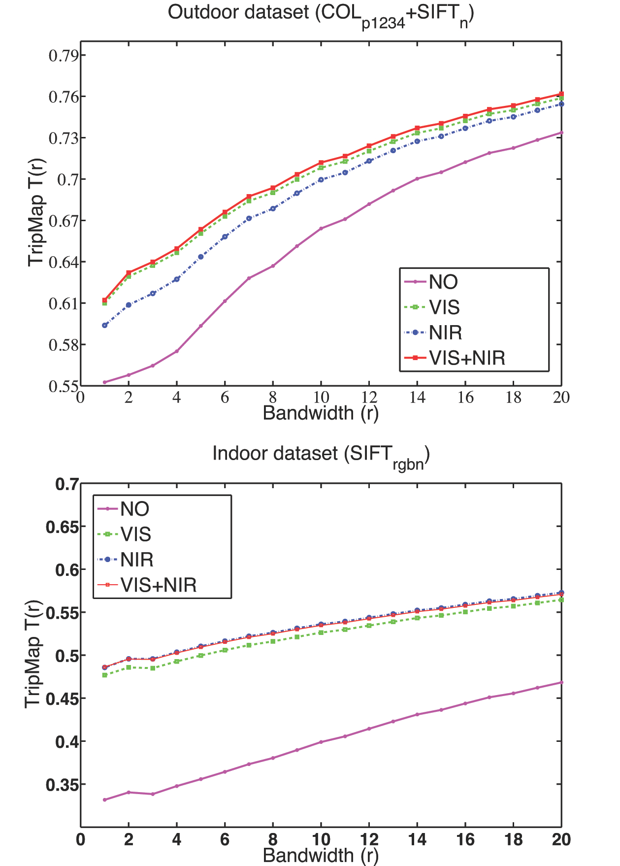
Figure 7: The TrimapAcc plots with different pairwise potentials using $COL_{p1234}+SIFT_{n}$ (top- for the outdoor dataset) respectively $SIFT_{rgbn}$ (bottom- for the indoor dataset) as unary potential.

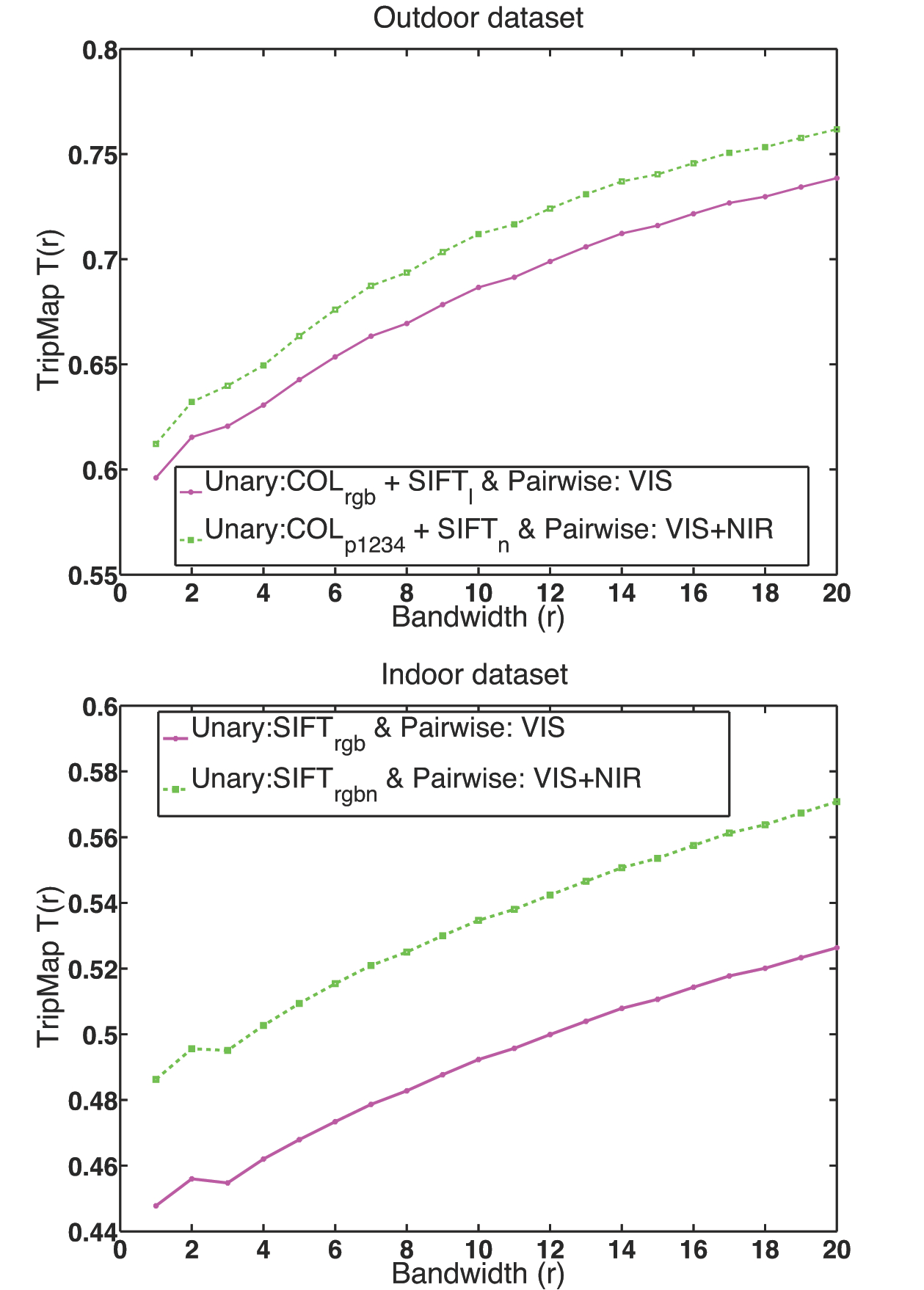
Figure 8: The TrimapAcc plots compare the border accuracy of the results of the visible only scenario and the proposed strategy, top- for the outdoor dataset and bottom- for the indoor dataset.

Results are shown in Table 2. First, we can see that for all the descriptors, the quality of semantic segmentation consistently increases when we consider both visible and NIR channels ($VIS+NIR$) in the pairwise potential, compared to using only visible or only NIR. Second, as expected, the regularization term (from any of the three strategies) improves the segmentation results obtained for any recognition model compared to the segmentation without regularization ($\lambda=0$, presented in Table 1). Finally, the ranking between the models with different descriptors is similar with or without regularization, given a regularization model (e.g.,  $VIS$ or $VIS+NIR$). This is again not surprising, as we use the same regularization term that is independent of the feature used in the recognition part. Again $COL_{rgbn}+SIFT_{n}$ and $COL_{p1234}+SIFT_{n}$ lead to the best performances in the case of the outdoor dataset, and $SIFT_{rgbn}$ performs best in the case of the indoor dataset, $COL_{rgbn}+SIFT_{n}$ being second best. Compared to the visible-only baselines $COL_{rgb}+SIFT_{l}$ or $SIFT_{rgb}$ with visible image-based regularization ($VIS$), they are significantly better and statistically different at the 95% confidence level according to the paired t-test applied to the score distributions.

For these experiments, we are mainly interested in the gain we obtain when comparing the $VIS$ or $NIR$-based regularization with the $VIS+NIR$-based regularization. Considering region-based evaluation measures, we can see only slight improvements even if the paired t-test often shows significant differences between the corresponding score distributions. Therefore, to better evaluate the gain obtained by combining the $NIR$ and $VIS$ channels in the regularization, we also evaluate some of these results with contour based measures.

We apply the trimap accuracy evaluation of kohli2009 (overall pixel accuracy in the neighborhood of object boundaries) and we show the results as a function of the boundary size in Figures 7 and 8. From these results, we can first notice the importance of the regularization. In both cases, any of the potentials that we use as regularizer leads to a significant improvement (statistically different at the 95% confidence level according to the paired t-test) on the results obtained by recognition alone ($NO$, for no pairwise). Comparing different edge potentials, we can see that, in outdoor scenes, the visible image leads to better segmentation than NIR image alone. Fixing the band $r$ at 5 pixels and running the t-test, we found that all $T(5)$ results are statistically different at a 95% confidence level.

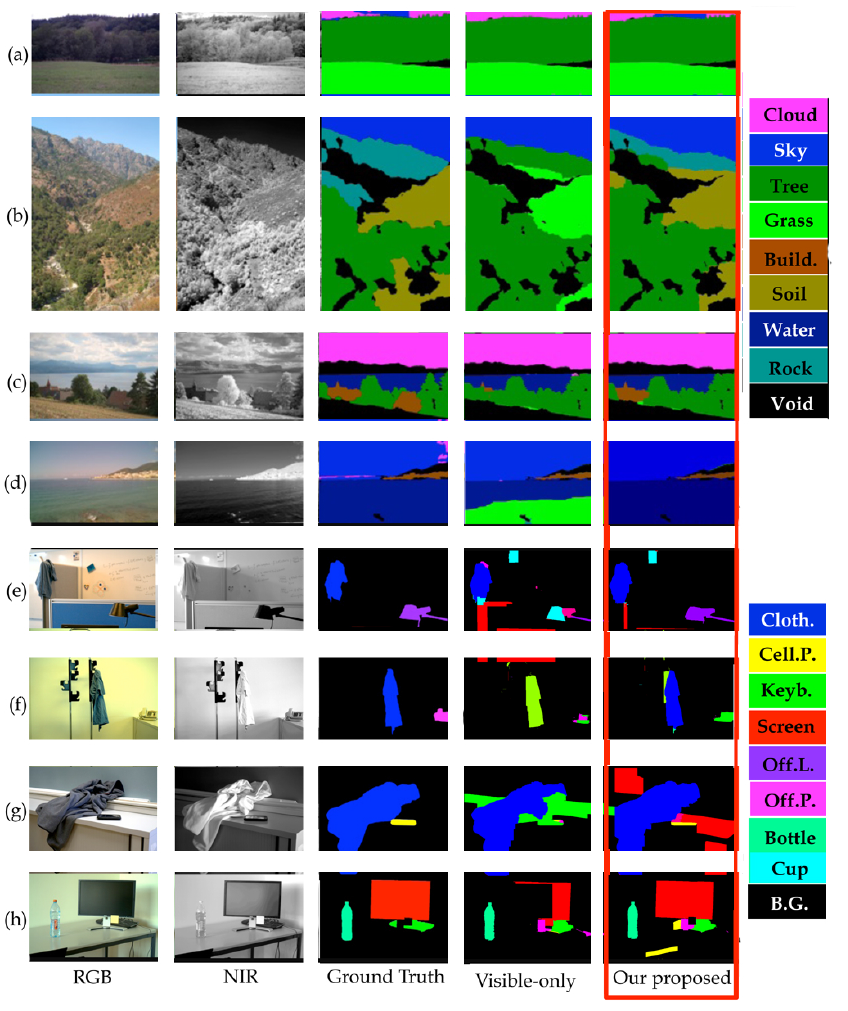
Figure 16: Sample segmentation results for the outdoor and the indoor datasets.

In order to show also some qualitative comparisons, Figure 16 shows a few segmentation results obtained with the visible baseline and the best visible + NIR setting. A visual inspection of these results allows to observe the positive qualitative influence of incorporating NIR information in the segmentation model.

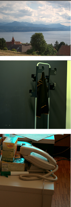
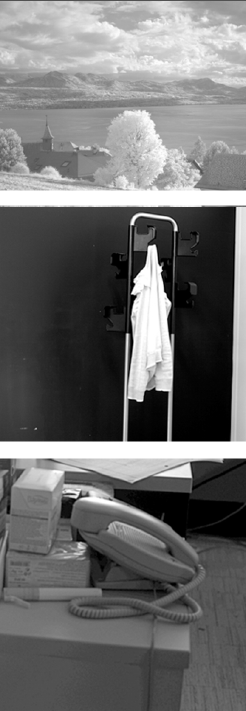
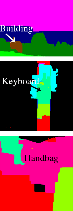
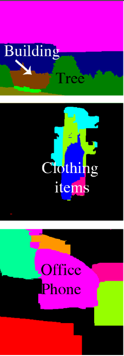
RGB	NIR	RGB-only results	RGB+NIR results

Figure 9: Examples from both outdoor and indoor datasets. Note that the material dependency of NIR images results helps both in recognition and a more accurate detection of object boundaries.

7 Class-based analyses and discussion

This section takes a deep dive into some of the results presented in the previous section in order to visualize, analyze and compare class-by-class results. We focus our analysis on the segmentation results obtained with the best visible baseline ($COL_{rgb}+SIFT_{l}$ for the outdoor dataset and $SIFT_{rgb}$ for the indoor dataset, with visible-only pairwise) and the best RGB+NIR integrated strategy ($COL_{p1234}+SIFT_{n}$ for the outdoor dataset and $SIFT_{rgbn}$ for the indoor dataset, with VIS + NIR pairwise).

We first show confusion matrices between the classes in Table 3 and Table 4. We also show qualitative results in Figure 9, Figure 10, Figure 11, Figure 12, Figure 13, Figure 14, Figure 15 and Figure 16, that we all discuss in detail below.

In general, in both datasets, we observe that borders are more precisely detected when NIR information is incorporated in the pairwise potential. This can be explained by the material dependency of NIR responses that might reduce the influence of wrong edges due to clutter, or might result in more contrasted edges between classes. This information, used in the regularization part of our model, helps better aligning borders between regions with the material change, as we can see in the examples of the Figure 9. We now analyze in depth the different classes, and discuss the datasets individually.

7.1 Outdoor scenes

First we discuss the results obtained for the outdoor dataset. This dataset contains mostly what is usually referred as “stuff”, e.g.,  background classes that are difficult to count. Based on Table 3 results, we can make the following observations.

Natural materials. First we discuss the relations between tree, grass and soil. Looking at the yellow boxes in Table 3, we observe the following. Tree and grass are more confused in NIR because they consist of the same material and have roughly the same texture. Grass and soil are less confused in NIR. The reason could be that the pigment in vegetation (Chlorophyll) is very reflective in the NIR part of the spectrum, whereas soil has a lower reflectance in this part that makes it appear very differently in the NIR representation of the scene. Soil and tree get more confused when NIR information is incorporated into our model. This can be explained by the fact that the wooden part of the tree has almost the same pixel values as soil, thus incorporating the $COL$ descriptor in the NIR part of the spectrum could be a source of confusion.

Table 3: Outdoor dataset. Left, confusion matrix of $COL_{p1234}+SIFT_{n}$ and visible+NIR pairwise. Right, confusion matrix for the best visible scenario ( $COL_{rgb}+SIFT_{l}$ with visible-only pairwise). Values on the diagonal of the confusion matrices correspond to the individual class accuracies.

Rock and grass get more confused in the absence of NIR information (see the red boxes in Table 3). Chlorophyll in grass is very reflective and discriminative in NIR images and rock is relatively more absorbent. Due to such material dependency of NIR images, incorporating this information into our model decreases the confusion of these two classes.

Water. Water has a mirror reflection in RGB images, so the reflection of close-by trees in water makes the $COL_{rgb}$ for the water class very close to $COL_{rgb}$ for tree. In NIR images, however, water is very absorbent and appears very dark, hence it is confused less with other classes of material. See Figure 10 for an illustration. In other words, even if in the RGB image, due to the reflection, the color or even the texture of the related region in the water lead to confusion with the reflected class (tree, sky, far away mountains), water has a unique appearance in the NIR leading to significantly improved recognition, compared to visible baseline (see the magenta boxes in Table 3 and the class accuracy of the water class on the diagonal).

Table 4: Indoor dataset. Left, confusion matrix of $SIFT_{rgbn}$ and visible+NIR pairwise. Right, confusion matrix for the best visible scenario ( $SIFT_{rgb}$ with visible-only pairwise). Values on the diagonal of the confusion matrices correspond to the individual class accuracies.

Haze. Finally, the benefit of using the NIR channel in the presence of haze can be observed particularly in the case of sky, tree and rock classes, the latter often representing mountains. As stated by Rayleigh’s law, the intensity of light scattered from very small particles ($<\lambda/10$) is inversely proportional to the fourth power of the wavelength $\lambda$ (i.e.,  $\propto 1/\lambda^{4}$) fredembach2008 . Particles in the air (haze) satisfy this condition and are therefore scattering more in the short-wavelength range of the spectrum. Thus, when images are captured in the NIR part of the spectrum, atmospheric haze is less visible and the sky becomes darker (see Figure 11). The “haze transparency” characteristic of NIR images results in sharper images for distant objects. In particular, vegetation at a distance in the visible image is smoothed and bluish, which can affect the performance of texture and color features in the classification task. The sharp and haze-free appearance of vegetation in NIR images helps with classification and leads to better segmentation (see also the diagonal in Table 3).

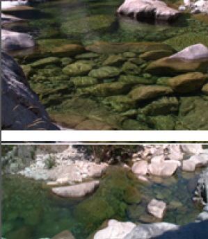
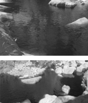
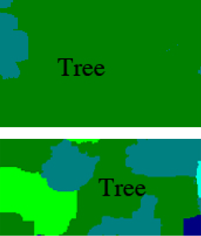
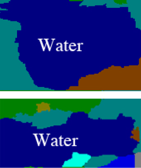
RGB	NIR	$COL_{rgb}+SIFT_{l}$	$COL_{pc1234}+SIFT_{n}$

Figure 10: In the visible only scenario, the class water is often confused with tree. The main reason is that the reflection of close-by trees or the presence of vegetation in the water make the color of the water very similar to the one from trees.

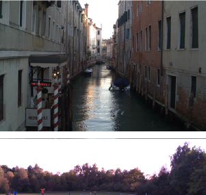
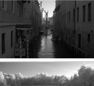
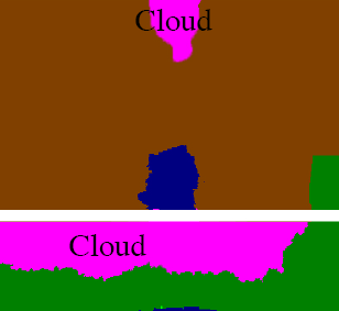
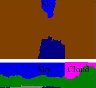
RGB	NIR	$COL_{rgb}+SIFT_{l}$	$COL_{pc1234}+SIFT_{n}$

Figure 11: Examples from the outdoor dataset. Note the better classification and recognition of $clouds$ and $sky$ when NIR information is incorporated.

7.2 Indoor scenes

The indoor dataset mostly contains categories that are related to object classes, also referred as “things”. From the results of Table 4 we can make the following observations.

Color distractors. The class screen is confused with colorful classes such as clothing item, handbag, and flowerpot, in the absence of NIR information (see the orange boxes in Table 4). Visible images of class screen contain many colorful patches (presence of colorful pictures on the screen), however, the appearance of this class is consistently the same in NIR images. As we can see in Figure 12 the content displayed on the screen is not visible anymore in the NIR image and hence incorporating this information yields to better recognition accuracy.

Fabric. Clothing item is confused with handbag in the visible-only scenario (see the red boxes in Table 4), mainly because such classes appear to look very similar (both in color values and texture measures). As these two classes are mostly made of different material (clothing item is mostly made of natural fabrics such as cotton or wool, or synthetic fabrics such as polyester or nylon, whereas handbag is made of suede or artificial suede, which are types of leather with a napped finish), they look significantly different in NIR images. See Figure 13 for an illustration.

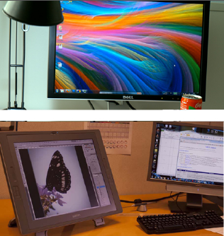
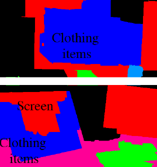
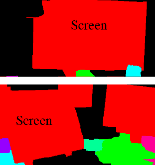
RGB	NIR	$SIFT_{rgb}$	$SIFT_{rgbn}$

Figure 12: Multi-spectral-SIFT ($SIFT_{rgbn}$) outperforms the best visible-only scenario in recognition of colorful classes where the material properties of the classes are different.

Man-made objects In the proposed scenario, cellphone is generally confused with the background class. In the visible only scenario, this class is more confused with keyboard as well as background. The low performance of our framework for this class is mostly due to the fact that the number of samples in this class is very low, so the classifier did not have enough training samples to learn from. A fewer number of training samples is also a factor for poor and unreliable performance for the cup, can, and bottle classes.

Surprisingly, the Office-phone class is significantly confused with the class handbag in the visible only scenario. However, when we add information from the NIR channel, this confusion significantly drops as shown in the red boxes in Table 4 due to the material differences of these classes, that is reliably captured by the NIR channel.

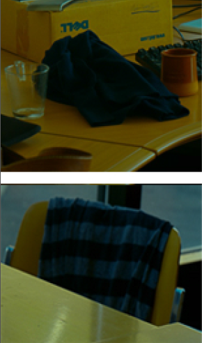
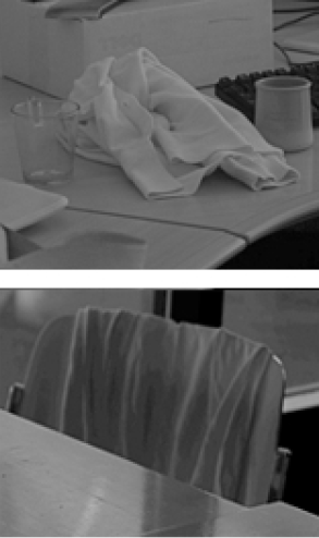
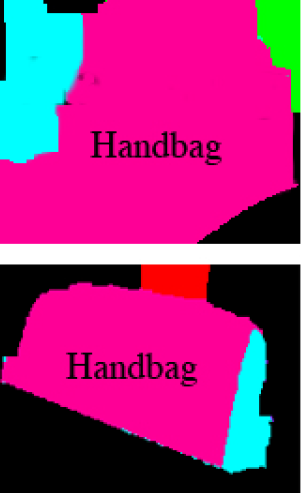
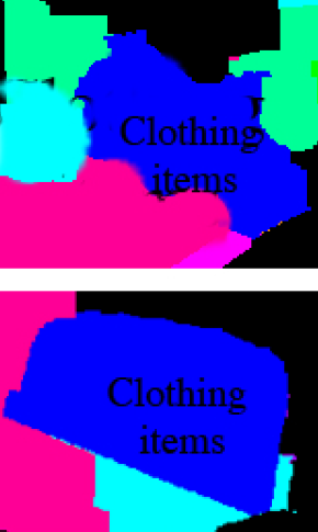
RGB	NIR	$SIFT_{rgb}$	$SIFT_{rgbn}$

Figure 13: Due to very different material characteristics of Clothing Item and Handbag, as well as material dependency of NIR information, the confusion of such classes is significantly less in presence of NIR information.

Vegetation. Incorporating NIR information in the segmentation task significantly improves the result of conventional visible-only scenario in the case of flowerpot because the very distinctive appearance of vegetation in NIR images helps the classifier to correctly recognize the class and detect the boundaries more accurately (see Figure 14 for illustration). The often higher contrast between this class and the background makes it easy for the CRF model to more accurately detect the boundaries of this class.

7.3 Summary

Summarizing, we can say that classes such as sky, grass, water and cloud in the outdoor dataset are better recognized by their intrinsic color. Capturing texture in a one-channel image and fusing it with the color information improves the results, mostly by distinguishing between grass and tree, or sky and water, where color is less discriminative. Figure 15 shows that incorporating material-dependent NIR images in the decorrelated PCA space for the $COL$ descriptor and fusing it with $SIFT$ features on the NIR image help to recognize such confusing classes.

RGB	NIR	$SIFT_{rgb}$	$SIFT_{rgbn}$

Figure 14: Due to very different material characteristics of vegetation, incorporating NIR information increases the accuracy of border detection.

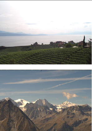
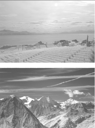
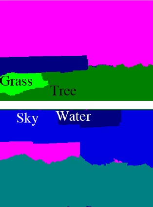
RGB	NIR	$COL_{rgb}+SIFT_{l}$	$COL_{pc1234}+SIFT_{n}$

Figure 15: The material dependency characteristics of NIR images helps to distinguish more accurately between the classes of material with the same intrinsic color. Higher contrast in the NIR images in the sky makes $SIFT_{n}$ a more discriminative feature in distinguishing between $sky$ and $water$.

By contrast, in the indoor scenes, most of the classes are man-made, and often are of different colors such as cloths or handbags. Hence, the color is less distinctive for recognizing the classes. This can explain why $COL$ features perform poorly compared to SIFT and similarly why multi-spectral SIFT outperforms the late fusion of $COL$ and $SIFT$ features. Figure 12 shows examples where incorporating $COL$ gives poor results in the recognition of colorful classes. There, texture is more intrinsic to the class, therefore multi-spectral-SIFT ($SIFT_{rgbn}$) outperforms the late fusion of $COL$ and $SIFT$.

8 Conclusion

In this paper our aim was to explore the idea that NIR information, captured from an ordinary digital camera, could be useful in semantic segmentation.

Therefore, we proposed to formulate the segmentation problem by using a CRF model, and we studied ways to incorporate the NIR cue in the recognition part and in the regularization part of our model. Considering the characteristics of NIR images, we have defined color and SIFT features on different combinations of the RGB and NIR channels.

To evaluate this framework, we have introduced a novel database of outdoor and indoor scene images, annotated at the pixel level, with 10 categories in the outdoor and 13 categories in the indoor scenes.

Through an extensive set of experiments, we have shown that integrating NIR as additional information, along with conventional RGB images indeed improves the segmentation results. We systematically studied the reasons for this improvement by taking into consideration the material characteristics and properties of the categories in the NIR wavelength range. In particular, the overall improvement is due to a large improvement for certain classes whose response in the NIR domain is particularly discriminant, such as water, sky or screen.

Acknowledgment. This work was supported by the Swiss National Science Foundation under grant number 200021-124796/1 and by the Xerox foundation.

References

- [1] G.A. Blackburn. Hyperspectral remote sensing of plant pigments. Journal of Experimental Botany, 58(4):855–867, 2007.
- [2] T. Blaschke. Object based image analysis for remote sensing. Journal of Photogrammetry and Remote Sensing, 65(1):2–16, 2010.
- [3] Y. Boykov and V. Kolmogorov. An experimental comparison of min-cut/max-flow algorithms for energy minimization in vision. IEEE Transactions on Pattern Analysis and Machine Intelligence, 26(9):1124–1137, 2004.
- [4] Y. Boykov, O. Veksler, and R. Zabih. Fast approximate energy minimization via graph cuts. IEEE Transactions on Pattern Analysis and Machine Intelligence, 23(11):1222–1239, 2001.
- [5] M. Brown and S. Süsstrunk. Multi-spectral sift for scene category recognition. In Conference on Computer Vision and Pattern Recognition, pages 177–184, 2011.
- [6] D.A. Burns and E.W. Ciurczak. Handbook of Near-infrared analysis. Marceld Ekkerin,Inc, 2001.
- [7] K. Chatfield, V. Lempitsky, A. Vedaldi, and A. Zisserman. The devil is in the details: an evaluation of recent feature encoding methods. In British Machine Vision Conference, pages 76.1–76.12, 2011.
- [8] S. Clinchant, G. Csurka, F. Perronnin, and J.M. Renders. XRCE’s participation to imageval. In ImageEval Workshop at CVIR, 2007.
- [9] R. Crabb, C. Tracey, A. Puranik, and J. Davis. Real-time foreground segmentation via range and color imaging. In Computer Vision and Pattern Recognition Workshops, pages 1–5, 2008.
- [10] G. Csurka, C. Dance, L. Fan, J. Willamowski, and C. Bray. Visual categorization with bags of keypoints. In Workshop on statistical learning in computer vision, ECCV, volume 1, page 22, 2004.
- [11] G. Csurka and F. Perronnin. An efficient approach to semantic segmentation. International Journal of Computer Vision, 95(2):198–212, 2011.
- [12] Gabriela Csurka, Diane Larlus, and Florent Perronnin. What is a good evaluation measure for semantic segmentation? In British Machine Vision Conference, 2013.
- [13] M. Everingham, LV Gool, C. Williams, and A. Zisserman. The pascal visual object classes challenge.
- [14] C. Fredembach and S. Süsstrunk. Colouring the near infrared. In Color Imaging Conference, pages 176–182, 2008.
- [15] P. Gunawardane, T. Malzbender, R. Samadani, A. McReynolds, D. Gelb, and J. Davis. Invisible light: Using infrared for video conference relighting. In International Conference on Image Processing, pages 4005–4008, 2010.
- [16] R. Hu, D. Larlus, and G. Csurka. On the use of regions for semantic image segmentation. In ICVGIP, 2012.
- [17] P. Kohli and M.P. Kumar. Energy minimization for linear envelope mrfs. In Conference on Computer Vision and Pattern Recognition, pages 1863–1870, 2010.
- [18] P. Kohli, L. Ladickỳ, and P.H.S. Torr. Robust higher order potentials for enforcing label consistency. International Journal of Computer Vision, 82(3):302–324, 2009.
- [19] V. Kolmogorov and R. Zabin. What energy functions can be minimized via graph cuts? IEEE Transactions on Pattern Analysis and Machine Intelligence, 26(2):147–159, 2004.
- [20] S.G. Kong, J. Heo, B.R. Abidi, J. Paik, and M.A. Abidi. Recent advances in visual and infrared face recognition a review. Computer Vision and Image Understanding, 97(1):103–135, 2005.
- [21] Philipp Krähenbühl and Vladlen Koltun. Efficient inference in fully connected crfs with gaussian edge potentials. In Advances in Neural Information Processing Systems, pages 109–117, 2011.
- [22] D. Krishnan and F. Fergus. Dark flash photography. In ACM Transactions on Graphics, SIGGRAPH 2009 Conference Proceedings, 2009.
- [23] B. Krishnapuram, L. Carin, M.A.T. Figueiredo, and A.J. Hartemink. Sparse multinomial logistic regression: Fast algorithms and generalization bounds. IEEE Transactions on Pattern Analysis and Machine Intelligence, 27(6):957–968, 2005.
- [24] A. Kulcke, C. Gurschler, G. Spock, R. Leitner, and M. Kraft. On-line classification of synthetic polymers using near infrared spectral imaging. Journal of near infrared spectroscopy, 11(1):71–81, 2003.
- [25] L. Ladicky, C. Russell, P. Kohli, and P. Torr. Graph cut based inference with co-occurrence statistics. European Conference on Computer Vision, pages 239–253, 2010.
- [26] L. Ladicky, C. Russell, P. Kohli, and P.H.S. Torr. Associative hierarchical crfs for object class image segmentation. In International Conference on Computer Vision, pages 739–746, 2009.
- [27] L’. Ladickỳ, P. Sturgess, K. Alahari, C. Russell, and P. Torr. What, where and how many? combining object detectors and crfs. In European Conference on Computer Vision, pages 424–437, 2010.
- [28] Diane Larlus, Jakob Verbeek, and Frédéric Jurie. Category level object segmentation by combining bag-of-words models with Dirichlet processes and random fields. International Journal of Computer Vision, 88(2):238–253, June 2010.
- [29] David G Lowe. Distinctive image features from scale-invariant keypoints. International journal of computer vision, 60(2):91–110, 2004.
- [30] Nigel J. W. Morris, Shai Avidan, Wojciech Matusik, and Hanspeter Pfister. Statistics of infrared images. In CVPR, 2007.
- [31] C. Pantofaru, C. Schmid, and M. Hebert. Object recognition by integrating multiple image segmentations. In European Conference on Computer Vision, pages 481–494, 2008.
- [32] F. Perronnin, J. Sánchez, and T. Mensink. Improving the fisher kernel for large-scale image classification. European Conference on Computer Vision, pages 143–156, 2010.
- [33] N. Plath, M. Toussaint, and S. Nakajima. Multi-class image segmentation using conditional random fields and global classification. In International Conference on Machine Learning, pages 817–824, 2009.
- [34] C. Rother, V. Kolmogorov, and A. Blake. Grabcut: Interactive foreground extraction using iterated graph cuts. In ACM Transactions on Graphics, volume 23(3), pages 309–314, 2004.
- [35] Z. Sadeghipoor, Y.M. Lu, and S. Susstrunk. Correlation-based joint acquisition and demosaicing of visible and near-infrared images. In International Conference on Image Processing, pages 3165–3168, 2011.
- [36] N. Salamati, D. Larlus, and G. Csurka. Combining visible and near-infrared cues for image categorisation. In British Machine Vision Conference, pages 49.1–49.11, 2011.
- [37] Neda Salamati, Clément Fredembach, and Sabine Süstrunk. Material Classification Using Color and NIR Images. In Color Imaging Conference, pages 216–222, 2009.
- [38] Neda Salamati, Diane Larlus, Gabriela Csurka, and Sabine S sstrunk. Semantic image segmentation using visible and near-infrared channels. In ECCV Workshop on Color and Photometry in Computer Vision, 2012.
- [39] Neda Salamati and Sabine Süstrunk. Material-Based Object Segmentation Using Near-Infrared Information. In Color Imaging Conference, pages 196–201, 2010.
- [40] J. Salvi, J. Pages, and J. Batlle. Pattern codification strategies in structured light systems. Pattern Recognition, 37(4):827–849, 2004.
- [41] L. Schaul, C. Fredembach, and S. Süsstrunk. Color image dehazing using the near-infrared. In IEEE International Conference on Image Processing, pages 1629–1632, 2009.
- [42] J. Shotton, M. Johnson, and R. Cipolla. Semantic texton forests for image categorization and segmentation. In Conference on Computer Vision and Pattern Recognition, pages 1–8, 2008.
- [43] J. Shotton, J. Winn, C. Rother, and A. Criminisi. Textonboost: Joint appearance, shape and context modeling for multi-class object recognition and segmentation. In European Conference on Computer Vision, pages 1–15, 2006.
- [44] S. Süsstrunk, C. Fredembach, and D. Tamburrino. Automatic skin enhancement with visible and near-infrared image fusion. In International Conference ACM Multimedia, pages 1693–1696, 2010.
- [45] R. Szeliski. Image alignment and stitching: A tutorial. Foundations and Trends® in Computer Graphics and Vision, 2(1):1–104, 2006.
- [46] Joost Van De Weijer and Cordelia Schmid. Coloring local feature extraction. In European Conference on Computer Vision, volume 3952, pages 334–348. Springer, 2006.
- [47] J. Verbeek and W. Triggs. Scene segmentation with crfs learned from partially labeled images. In Advances in Neural Information Processing Systems, 2007.
- [48] V. Walter. Object-based classification of remote sensing data for change detection. ISPRS Journal of Photogrammetry and Remote Sensing, 58(3):225–238, 2004.
- [49] L. Yang, P. Meer, and D.J. Foran. Multiple class segmentation using a unified framework over mean-shift patches. In Conference on Computer Vision and Pattern Recognition, pages 1–8, 2007.
- [50] X. Zhang, T. Sim, and X. Miao. Enhancing photographs with near infra-red images. In Conference onComputer Vision and Pattern Recognition, pages 1–8, 2008.
- [51] W. Zhou, G. Huang, A. Troy, and ML Cadenasso. Object-based land cover classification of shaded areas in high spatial resolution imagery of urban areas: A comparison study. Remote Sensing of Environment, 113(8):1769–1777, 2009.