Consistency Relations for Large Field Inflation

Abstract

Consistency relations for chaotic inflation with a monomial potential and natural inflation and hilltop inflation are given which involve the scalar spectral index $n_{s}$, the tensor-to-scalar ratio $r$ and the running of the spectral index $\alpha$. The measurement of $\alpha$ with $O(10^{-3})$ and the improvement in the measurement of $n_{s}$ could discriminate monomial model from natural/hilltop inflation models. A consistency region for general large field models is also presented.

I Introduction

The possible detection of the primordial B-mode bicep2 has changed the landscape of models of inflation. The scene has completely changed from small inflation models to large field inflation models, although the plot thickens Seljak . Awaiting for the polarization results by Planck, in the meantime, we may entertain the possibility of large field inflation and shall speculate on the way to further narrow down the models of inflation. Then the analysis would be inevitably model-dependent. However, we would like to minimize the dependence on model parameters. So, we consider a relation which a given (single field) inflation model predicts independent of model parameters, in the same spirit as the single-field inflationary consistency relation ll .

II Consistency Relations for Large Field Inflation

Large field models of inflation inhabit the region where the scalar spectral index is red $n_{s}<1$ and the tensor-to-scalar ratio is relatively large $r\gtrsim 0.1$ dodelson . Chaotic inflation with a monomial potential chaotic and natural inflation natural are typical examples of (single field) large field inflation. So, we attempt to derive consistency relations for these models which hold independent of model parameters. We use the units of $M_{\rm pl}=1/\sqrt{8\pi G}=1$.

II.1 Monomial Potential

First, we consider chaotic inflation with a monomial potential:

$$V=\lambda\phi^{n},$$ (1)

where we assume $\phi>0$ and the power index $n(>0)$ needs not be integer and can be fractional (or real) number like $2/3$ as in axion monodromy inflation model silverstein . In any case, $n$ is a constant and can be written as $n={d\ln V}/{d\ln\phi}$. Differentiating $n$ with respect $\phi$, we have

$$\phi=\frac{VV^{\prime}}{V^{\prime 2}-VV^{\prime\prime}},$$ (2)

where $V^{\prime}=dV/d\phi$, and so on. Further taking the derivative, we obtain

$$VV^{\prime 2}V^{\prime\prime}-2V^{2}V^{\prime\prime 2}+V^{2}V^{\prime}V^{\prime\prime\prime}=0\,.$$ (3)

In addition, since we assume $\phi>0$ (and hence $V^{\prime}>0$), from Eq. (2) we require

$$V^{\prime 2}-VV^{\prime\prime}>0\,.$$ (4)

In terms of the slow-roll parameters

$$\epsilon\equiv\frac{1}{2}\left(\frac{V^{\prime}}{V}\right)^{2},\quad\eta\equiv\frac{V^{\prime\prime}}{V},\quad\xi\equiv\frac{V^{\prime}V^{\prime\prime\prime}}{V^{2}}\,,$$ (5)

these relations Eq. (3) and Eq. (4) can be rewritten as

$$2\epsilon\eta-2\eta^{2}+\xi=0\quad{\rm and}\quad 2\epsilon>\eta\,.$$ (6)

Using inflationary observables related to the slow-roll parameters, the scalar spectral index $n_{s}$, the tensor-to-scalar ratio $r$ and the running of the spectral index $\alpha$

$$n_{s}-1=-6\epsilon+2\eta,\quad r=16\epsilon,\quad\alpha=\frac{dn_{s}}{d\ln k}=16\epsilon\eta-24\epsilon^{2}-2\xi\,,$$ (7)

Eq. (6) become relations among observables

$$\alpha=-(1-n_{s})^{2}+\frac{1}{8}r(1-n_{s})\quad{\rm and}\quad 1-n_{s}>\frac{1}{8}r\,,$$ (8)

which we call consistency relations for monomial chaotic inflation which may be reminiscent of the consistency relation for a single field inflation ll . The second inequality implies the red spectrum: $n_{s}<1$. Note that Eq. (8) holds for chaotic inflation with a monomial potential irrespective of the power index $n$.

II.2 Natural Inflation

Next, we consider natural inflation

$$V=V_{0}\left(1-\cos\left(\frac{\phi}{f}\right)\right),$$ (9)

where we assume $0<\phi<\pi f$ and $f$ is the decay constant and $V_{0}$ is related with the breaking scale of the global symmetry for axion. For $f\gg 1$ the potential becomes indistinguishable from a quadratic potential.

$V_{0}$ can be written as

$$V_{0}^{2}=(V+f^{2}V^{\prime\prime})^{2}=(fV^{\prime})^{2}+(f^{2}V^{\prime\prime})^{2},$$ (10)

and $f$ can be written as $f^{2}=-V^{\prime}/V^{\prime\prime\prime}$. Hence, using the slow-roll parameters, we obtain a relation

$$4\epsilon^{2}-4\epsilon\eta+\xi=0.$$ (11)

Moreover, since $V^{\prime}>0$ and $V^{\prime\prime\prime}<0$, $\xi<0$ is required. Then, in terms of observables, we obtain relations

$$\alpha=\frac{1}{32}r^{2}-\frac{1}{4}r(1-n_{s})\quad{\rm and}\quad\alpha>\frac{3}{32}r^{2}-\frac{1}{2}r(1-n_{s})$$ (12)

which we call consistency relations for natural inflation. Note that Eq. (12) holds for natural inflation irrespective of the value of $f$. Note that the inequality is saturated when $\alpha=-r^{2}/32$ which corresponds to the relation for a quadratic potential. We also note that the second inequality can also be derived from the inequality

$$r<4(1-n_{s})\,,$$ (13)

which follows from $\cos\left(\phi/f\right)=\eta/(2\epsilon-\eta)<1$.

II.3 Extra Natural Inflation

The potential of extranatural inflation extranatural is given by

$$V(\phi)=V_{0}\left[1-\sum_{n=1}^{\infty}\frac{\cos\left(n\frac{\phi}{f}\right)}{n^{5}}\right].$$ (14)

For simplicity, following lim , we neglect the higher $n$-terms for $n\geq 2$ to calculate $V,V^{\prime}$ and $V^{\prime\prime}$ for both $\epsilon$ and $\eta$ since they are suppressed by $1/n^{5},1/n^{4}$ or $1/n^{3}$, but we include higher order terms to calculate $V^{\prime\prime\prime}$ (and higher derivatives). Then $\xi$ is given approximately by lim ,

$$\displaystyle{\xi=\frac{\left[\ln\left(\frac{\phi}{f}\right)-1\right]\left(\frac{\phi}{f}\right)\sin\left(\frac{\phi}{f}\right)}{f^{4}\left[1-\cos\left(\frac{\phi}{f}\right)\right]^{2}}},$$ (15)

where

$$\cos\left(\frac{\phi}{f}\right)=\frac{\eta}{2\epsilon-\eta}\,,$$ (16)

and $\cos\left(\frac{\phi}{f}\right)<1$ gives the same condition as   (13) under this approximation. From Eq. (15) and Eq. (16) together with $f^{-2}=2(\epsilon-\eta)$, $\xi$ is written as a function of $\epsilon$ and $\eta$, and hence we obtain a relation among $n_{s},r$ and $\alpha$ which is too complicated to show here. Note that the prediction of $r=16\epsilon$ could roughly have a 10 $\%$ error at most because $|\Delta r/r|=|\Delta\epsilon/\epsilon|\sim 2|\Delta V^{\prime}/V^{\prime}|\sim\Sigma_{n=2}^{\infty}\frac{2}{n^{4}}\sin(n\phi/f)\ll 1/2^{3}$. The validity of this approximation was checked in detail by Ref.lim .

II.4 Hilltop Inflation

We can also derive a consistency relation for hilltop hilltop (or symmetry breaking kl ) inflation

$$V(\phi)=\frac{\lambda}{4}\left(\phi^{2}-v^{2}\right)^{2}\,.$$ (17)

For $\phi\gg v$, the potential becomes a quartic potential. A simple calculation gives

$$3\epsilon^{2}-3\epsilon\eta+\xi=0.$$ (18)

Moreover, since $9V^{\prime}V^{\prime\prime\prime}-6V^{\prime\prime 2}=-6\lambda^{2}(3\phi^{2}+v^{2})v^{2}<0$, we have an inequality

$$\xi-\frac{2}{3}\eta^{2}<0\,.$$ (19)

In terms of $\alpha,r$ and $n_{s}$, consistency relations become

$$\alpha=\frac{3}{64}r^{2}-\frac{5}{16}r(1-n_{s})\quad{\rm and}\quad\alpha>-\frac{1}{3}(1-n_{s})^{2}+\frac{3}{64}r^{2}-\frac{1}{4}r(1-n_{s})\,.$$ (20)

Note that the inequality is saturated at $\alpha=-(3/256)r^{2}$ which precisely corresponds to the relation for a quartic potential.

In Fig. 1, we show these relations in $(r,\alpha)$ plane for $0.955<n_{s}<0.965$ which should be possible by measurements by Planck planck . The shaded regions (blue, green, red, orange) are the relations for monomial potential, natural, extranatural, symmetry breaking potential, respectively. For each region, the upper (lower) curve is for $n_{s}=0.965(0.955)$. The middle solid curves are for $n_{s}=0.96$. Blue dashed curved are for $n=2/3,2$ from left to right, and green or red dashed curves are for $f=7,10$ from left to right, although for $f=10$ green dashed curve almost coincides with red dashed curve. In Fig. 2, we also show the relations for for $n_{s}=0.96\pm 0.001$ which might be possible by future observations of the fluctuations of the 21 cm line of neutral hydrogen kohri .

The current constraint on $\alpha$ from Planck is $\alpha=-0.019\pm 0.010$ PlanckXVI . The measurement of $\alpha$ with the precision of $O(10^{-3})$, which would be possible kohri by future observations of the 21 cm line by SKA ska or by Omniscope omniscope , could discriminate chaotic inflation with a monomial model from natural/extranatural/hilltop models. Further, the measurement of $\alpha$ with a precision of $O(10^{-4})$, which would be possible kohri by measurements by CMBPol cmbpol combined with Omniscope omniscope , could discriminate natural inflation from hilltop inflation.

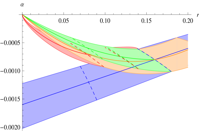
Figure 1: Consistency relations for $0.955<n_{s}<0.965$ in $(r,\alpha)$ plane. The shaded regions (blue, green, red, orange) are the relations for monomial, natural, extranatural, symmetry breaking potential, respectively. For each region, the upper (lower) curve is for $n_{s}=0.965(0.955)$. The middle solid curves are for $n_{s}=0.96$. Blue dashed curved are for $n=2/3,2$ from left to right, and green or red dashed curves are for $f=7,10$ from left to right.

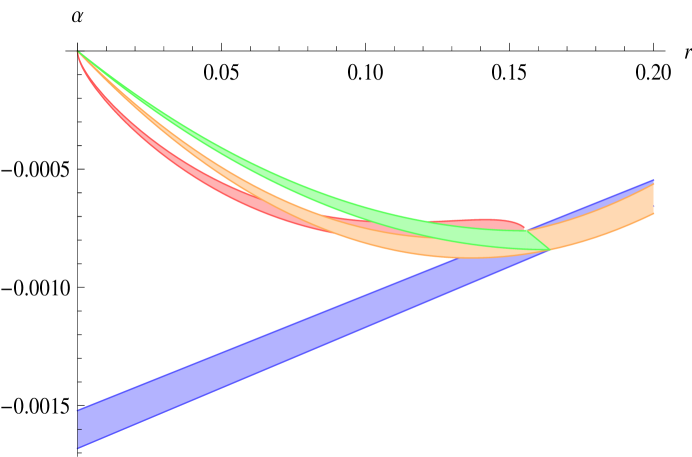
Figure 2: Same as Fig. 1 but for $n_{s}=0.96\pm 0.001$.

II.5 More General Large Field Models

For more general models, firstly we need to define the large field model. Following dodelson , we define the large field model by

$$0<\eta<2\epsilon,$$ (21)

where the first inequality follows from the convexity of $V$: $V^{\prime\prime}>0$ and the second inequality from the exponential function (power-law inflation). In this case, $\alpha$ is limited by

$$-\frac{3}{32}r^{2}-2\xi<\alpha<\frac{1}{32}r^{2}-2\xi.$$ (22)

The inequality involves an unknown parameter $\xi$. However, since $\xi$ is the second order slow-roll parameter, it may be at most of $O(N^{-2})\sim O(10^{-3})$, where $N\sim 50\sim 60$ is the e-folding number during inflation. Therefore, if we vary $\xi$ from $-10^{-3}$ to $10^{3}$, the region bounded by

$$-\frac{3}{32}r^{2}-2\times 10^{-3}<\alpha<\frac{1}{32}r^{2}+2\times 10^{3},$$ (23)

is the allowed region for general large field models defined by Eq. (21). The region is shown in Fig. 3 together with the consistency relations for monomial and natural inflation shown in Fig. 1. In any case, the measurement of $\alpha$ with the precision of $O(10^{-3})$ is required to probe the region. Conversely, the measurement of $|\alpha|>3\times 10^{-3}$ would refute the large field models defined by Eq. (21).

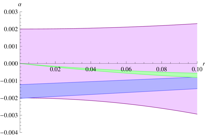
Figure 3: Consistency region for general large field models for $|\xi|<10^{-3}$. The consistency relations for monomial and natural inflation in Fig. 1 are also shown.

III Summary

We have provided consistency relations for chaotic inflation with a monomial potential Eq. (8), for natural inflation Eq. (12) and for hilltop inflation Eq. (20) which relate $n_{s},r$ and $\alpha$. We have also given an inequality Eq. (23) for large field models defined by Eq. (21). We find that the running of the spectral index $\alpha$ as well as the tensor-to-scalar ratio $r$ is the key observables to discriminate monomial models from natural/extranatural inflation models. We should emphasize that $n_{s}$ and $r$ without using $\alpha$ monomial models cannot be discriminate from natural/extranatural inflation unless we assume the power index of monomial potential and the e-folding number $N$. Even for smaller $r$, $(r,n_{s})$ of natural inflation with larger $N$ can overlap with monomial with lower $N$. We stress that $N$ is not a measurable quantity.

It would be interesting to extend such relations to other large field models, such as polynomial models, but that would involve the running of $\alpha$. It would also be interesting to investigate inflation models with non-canonical kinetic terms. We hope that our consistency relations would help to pin down the inflation model.

References

- (1) P. A. R. Ade et al. [BICEP2 Collaboration], Phys. Rev. Lett. 112, 241101 (2014) [arXiv:1403.3985 [astro-ph.CO]].
- (2) M. J. Mortonson and U. Seljak, arXiv:1405.5857 [astro-ph.CO]; R. Flauger, J. C. Hill and D. N. Spergel, arXiv:1405.7351 [astro-ph.CO].
- (3) A. R. Liddle and D. H. Lyth, Phys. Lett. B 291, 391 (1992) [arXiv:astro-ph/9208007].
- (4) P. Creminelli, D. Lopez Nacir, M. Simonovic, G. Trevisan and M. Zaldarriaga, arXiv:1404.1065 [astro-ph.CO].
- (5) S. Dodelson, W. H. Kinney and E. W. Kolb, Phys. Rev. D 56, 3207 (1997) [astro-ph/9702166].
- (6) A. D. Linde, Phys. Lett. B 129, 177 (1983).
- (7) K. Freese, J. A. Frieman and A. V. Olinto, Phys. Rev. Lett. 65, 3233 (1990).
- (8) E. Silverstein and A. Westphal, Phys. Rev. D 78, 106003 (2008) [arXiv:0803.3085 [hep-th]].
- (9) K. Kohri and T. Matsuda, arXiv:1405.6769 [astro-ph.CO].
- (10) N. Arkani-Hamed, H. -C. Cheng, P. Creminelli and L. Randall, Phys. Rev. Lett. 90, 221302 (2003) [hep-th/0301218].
- (11) K. Kohri, C. S. Lim and C. -M. Lin, arXiv:1405.0772 [hep-ph].
- (12) L. Boubekeur and D. .H. Lyth, JCAP 0507, 010 (2005) [hep-ph/0502047].
- (13) A. D. Linde, Phys. Lett. B 132, 317 (1983);
- (14) J. Tauber et al. [Planck Collaboration], astro-ph/0604069.
- (15) K. Kohri, Y. Oyama, T. Sekiguchi and T. Takahashi, JCAP 1310, 065 (2013) [arXiv:1303.1688 [astro-ph.CO]].
- (16) P. A. R. Ade et al. [Planck Collaboration], arXiv:1303.5076 [astro-ph.CO].
- (17) http://www.skatelescope.org/; G. Mellema, L. V. E. Koopmans, F. A. Abdalla, G. Bernardi, B. Ciardi, S. Daiboo, A. G. de Bruyn and K. K. Datta et al., Exper. Astron. 36, 235 (2013) [arXiv:1210.0197 [astro-ph.CO]].
- (18) M. Tegmark and M. Zaldarriaga, Phys. Rev. D 82, 103501 (2010) [arXiv:0909.0001 [astro-ph.CO]].
- (19) D. Baumann et al. [CMBPol Study Team Collaboration], AIP Conf. Proc. 1141, 10 (2009) [arXiv:0811.3919 [astro-ph]].