Evolution of the Coronal Magnetic Configurations Including a Current-Carrying Flux Rope in Response to the Change in the Background Field

Abstract

We investigate equilibrium height of the flux rope, and its internal equilibrium in a realistic plasma environment by carrying out numerical simulations of the evolution of systems including a current-carrying flux rope. We find that the equilibrium height of the flux rope is approximately a power-law function of the relative strength of the background field. Our simulations indicate that the flux rope can escape more easily from a weaker background field. This further confirms the catastrophe in the magnetic configuration of interest can be triggered by decrease of strength of the background field. Our results show that it takes some time to reach internal equilibrium depending on the initial state of the flux rope. The plasma flow inside the flux rope due to the adjustment for the internal equilibrium of the flux rope remains small and does not last very long when the initial state of the flux rope commences from the stable branch of the theoretical equilibrium curve. This work also confirms the influence of the initial radius of flux rope on its evolution, the results indicate that the flux rope with larger initial radius erupts more easily. In addition, by using the realistic plasma environment and much higher resolution in our simulations, we notice some different characters compared to previous studies in Forbes (1990).

1 Introduction

The most intense energetic activity in the solar system may be solar coronal mass ejection (CME). During the process, a large number of magnetized energetic plasmas (with mass of up to $10^{16}$ g and energy of $10^{32}$ erg) are ejected into the interplanetary space within a short timescale, and hence disturb spatial and planetary magnetic field and significantly affect satellite operation, aviation power, human space exploration, communication and so on (Chen et al. 2002, Schwenn 2006, Pulkkinen 2007, Lin 2007, Chen 2011, Mei et al. 2012b, Shen et al. 2013, Li et al. 2013, and references therein).

It is generally believed that two processes would have been involved in the intense solar activities and eruptions. The first one is called storage phase, in which the magnetic flux transported from the photosphere is slowly accumulated into the corona, leading to the gradual increase of the magnetic energy in the corona. The timescale of the magnetic storage phase is typically several days, so this phase can be considered as evolving through a series of equilibria in quasi-static processes. When the stored magnetic energy surpasses the critical values, the equilibrium will be broken, and the eruptive phase, i.e. the second process, will occur. The system in this phase will expand promptly in a dynamic timescale of a few minutes (i.e. in Alfv$\acute{e}$n time scales) due to loss of balance. Transition from the quasi-static evolution to the dynamic phase constitutes the so-called catastrophe (e.g. Forbes & Isenberg 1991; Isenberg et al. 1993; Forbes & Priest 1995; Forbes 1994, 2000; Lin & Forbes 2000; Lin et al. 2006; Yu 2012, and references therein).

It is well known that the motion of the photospheric material transports the energy to the coronal magnetic field for driving the eruption, so triggering and the consequent propagation of CMEs are governed by the changes in the photosphere. Recently, based on MHD simulation, some authors (Zhang et al. 2011, Welsch et al. 2009, Kusano et al. 2012, Kliem et al. 2013, and references therein) investigated how the physical features in the photosphere influence the evolution in the coronal magnetic configuration as well we the initiation of CMEs. However, without detailed observations and theoretical simulations, the determinations for the onset of CMEs still remain unclear.

The decay of the background magnetic field may be a cause to deviate the CME progenitor structure from the equilibrium, as shown in Isenberg et al. (1993) and Lin et al. (1998). This decay could be a consequent of the magnetic diffusion that leads to the formation, as well as the eruption, of flux rope (Mackay & van Ballegooijen 2006). Gradually decreasing the background field may also cause the state of the flux rope to transit catastrophically from the old equilibrium to the new one (Forbes & Isenberg 1991;Isenberg et al. 1993). Lin et al. (1998) analytically extended this work to include the curvature force that creates an additional outward force, and further realized that, in addition to the impact of the background field, the radius of flux rope plays an important role in its eruption. However, these results are constrained by the analytical method. Although Wang et al. (2009) and Mei et al. (2012a) numerically investigated the evolution of flux rope, the initial distribution of the plasma density in the background field in their simulations are a little bit far from the realistic case.

We in this paper will numerically investigate the evolution of the magnetic configuration and the current-carrying flux rope with the consideration of the gravitational stratification effect and more realistic distribution of the plasma density in the background field, which is crucial for the generation of CMEs, the understanding of the catastrophe model for CMEs, and therefor can allow us to further study the solar-terrestrial relationship. In addition, a number of numerical experiments have also been carried out to study how the variation of the background fields triggers the eruption of the flux rope and the influence of the radius of the flux rope on the eruption in detail. In §2, we describe the physical model, formulae and numerical approaches. The numerical results are presented in §3. We make a discussion and draw conclusions in §4.

2 Physical Model and Numerical Method

We consider that the prominence or the filament floating in the corona can be represented by a current-carrying flux rope, and the photospheric background field is represented by a line dipole below the photosphere. We assume a two-dimensional magnetic configuration in the semi-infinite $x$-$y$ plane in the Cartesian coordinates. In the coordinates, $y=0$ is assumed to be the boundary between the photosphere and the chromosphere, $y>0$ corresponds to the chromosphere and the corona. The location of the flux rope in our simulations is assumed to be $y=h$ above the boundary $y=0$, and the depth of the photospheric background field is $y=-d$ below $y=0$. The empirical atmosphere model described in Sittler & Guhathakurta (1999) (hereafter S&G) is used for the initial background field density $\rho_{0}(y)$. The evolution of the magnetic system should satisfy the following ideal magnetohydrodynamic (MHD) equations:

$$\begin{split}&\frac{\textrm{D}\rho}{\textrm{D}t}+\rho\nabla\cdot\textbf{v}=0,\\ &\rho\frac{\textrm{D}\textbf{v}}{\textrm{D}t}=-\nabla p+\frac{1}{c}\textbf{J}\times\textbf{B}+\rho\frac{GM_{\bigodot}}{(R_{\bigodot}+y)^{2}},\\ &\rho\frac{\textrm{D}}{\textrm{D}t}(e/\rho)=-p\nabla\cdot\textbf{v},\\ &\frac{\partial\textbf{B}}{\partial t}=\nabla\times(\textbf{v}\times\textbf{B}),\\ &\textbf{J}=\frac{c}{4\pi}\nabla\times\textbf{B},\\ &p=(\gamma-1)e,\\ &p=\rho kT/m_{p},\end{split}$$ (1)

where B represents the magnetic field, J the electric current density, $\rho$ the mass density, v the velocity of the flow, $p$ the gas pressure, $e$ the internal energy density, $\gamma$ the ratio of specific heats, $G$ the gravitational constant, $M_{\odot}$ the solar mass, $R_{\odot}$ the solar radius, $m_{p}$ the proton mass. Equations in (1) are numerically solved by using the ZEUS-2D MHD code described in Stone & Norman (1992a, 1992b,1992c).

The magnetic configuration in our simulations is composed of the current-carrying flux rope, the image of the current inside the flux rope, and the background magnetic field. We assume that the background field is generated by a line dipole below the bottom of the chromosphere (Forbes 1990; Wang et al. 2009). The relative strength of the dipole field $M$ can be defined by a dimensionless parameter $M=m/(Id)$, which is related to the ratio of the strength of the dipole field $m$ and the product of the filament current $I$ and the depth $d$ of the dipole field.

The initial magnetic configuration from which the eruption occurs is given by

$$B_{x} = B_{\phi}(R_{-})(y-h_{0})/R_{-}-B_{\phi}(R_{+})(y+h_{0})/R_{+}$$ (2)

$$- B_{\phi}(r+\Delta/2)Md(r+\Delta/2)[x^{2}-(y+d)^{2}]/R^{4}_{d},$$

$$B_{y} = -B_{\phi}(R_{-})x/R_{-}+B_{\phi}(R_{+})x/R_{+}$$ (3)

$$- B_{\phi}(r+\Delta/2)Md(r+\Delta/2)2x(y+d)/R^{4}_{d},$$

with

$$R^{2}_{\pm} = x^{2}+(y\pm h_{0})^{2},$$

$$R^{2}_{d} = x^{2}+(y+d)^{2}.$$

As for the initial background plasma density $\rho_{0}(y)$, we use an empirical atmosphere S&G model:

$$\begin{split}&\rho_{0}(y)=\rho_{00}f(y),\\ &f(y)=a_{1}z^{2}(y)e^{a_{2}z(y)}[1+a_{3}z(y)+a_{4}z^{2}(y)+a_{5}z^{3}(y)],\\ &z(y)=\frac{R_{\odot}}{R_{\odot}+y},\end{split}$$ (4)

where $\rho_{00}=1.672\times 10^{-13}$ g cm^-3, which is about one order of magnitude smaller than that in our previous work ($\sim 10^{-12}$ g cm^-3, Wang et al. 2009), and $a_{1}=0.001272$, $a_{2}=4.8039$, $a_{3}=0.29696$, $a_{4}=-7.1743$, $a_{5}=12.321$. The height $y$ is measured from the surface of the Sun. Equations (4) give a slowly decreasing density distribution $f(y)$ for the atmosphere in the lower corona. This density distribution was supported by the radio observations of type III bursts over wide frequency band of a few kHz to 13.8 MHz (Leblanc et al. 1998; Lin 2002). The density model considered in this work is more realistic than that used in previous work (Wang et al. 2009; Mei et al. 2012a).

For the initial background atmosphere, there is a balance between pressure gradient of gas and the gravity

$$\nabla p_{0}(y)=-\rho_{0}(y)\frac{GM_{\odot}}{(R_{\odot}+y)^{2}}.$$ (5)

From equations (4) and (5), we can get the relation between the initial background pressure $p_{0}(y)$, and the temperature distribution $T_{0}(y)$ as follows

$$p_{0}(y)=\frac{\rho_{0}(y)}{m_{p}}kT_{0}(y),$$ (6)

where $k$ is the Boltzmann constant.

Subsequently the initial total pressure, including the gas pressure and the magnetic pressure, and the mass density can be written as

$$\begin{split}&p=p_{0}-\int^{\infty}_{R_{-}}B_{\phi}(R)j(R)dR,\\ &\rho=\rho_{0}(p/p_{0})^{1/\gamma}.\end{split}$$ (7)

$B_{\phi}(R)$ in equations (2), (3) and (7) is determined by the electric current density distribution $j(R)$ inside the flux rope, and reads as

$$B_{\phi}(R) = -\frac{2\pi}{c}j_{0}R,\hskip 5.69054pt{\mbox{f}or}\hskip 5.69054pt0\leq R\leq r-\Delta/2,$$

$$B_{\phi}(R) = -\frac{2\pi j_{0}}{cR}\left\{\frac{1}{2}\left(r-\frac{\Delta}{2}\right)^{2}-\left(\frac{\Delta}{\pi}\right)^{2}+\frac{1}{2}R^{2}+\frac{\Delta R}{\pi}\sin\left[\frac{\pi}{\Delta}\left(R-r+\frac{\Delta}{2}\right)\right]\right.$$

$$+ \left.\left(\frac{\Delta}{\pi}\right)^{2}\cos\left[\frac{\pi}{\Delta}\left(R-r+\frac{\Delta}{2}\right)\right]\right\},\hskip 5.69054pt{\mbox{f}or}\hskip 5.69054ptr-\Delta/2<R<r+\Delta/2,$$

$$B_{\phi}(R) = -\frac{2\pi j_{0}}{cR}\left[r^{2}+(\Delta/2)^{2}-2(\Delta/\pi)^{2}\right],\hskip 5.69054pt{\mbox{f}or}\hskip 5.69054ptr+\Delta/2\leq R<\infty;$$

$$j(R) = j_{0},\hskip 5.69054pt{\mbox{f}or}\hskip 5.69054pt0\leq R\leq r-\Delta/2,$$

$$j(R) = \frac{j_{0}}{2}{\cos[\pi(R-r+\Delta/2)/\Delta]+1},\hskip 5.69054pt{\mbox{f}or}\hskip 5.69054ptr-\Delta/2<R<r+\Delta/2,$$

$$j(R) = 0,\hskip 5.69054pt{\mbox{f}or}\hskip 5.69054ptr+\Delta/2\leq R<\infty.$$ (8)

We take the computational domain to be $(-4L,4L)\times(0,8L)$ with $L=10^{5}$ km, and the grid points to be $800\times 800$. A line-tied condition is applied to the bottom boundary at $y=0$, while the open boundary condition is used for the other three. The initial values of the parameters in our simulations are listed in Table 1.

Table 1: The initial values for the important parameters in the numerical experiments.

$\rho_{00}=1.672\times 10^{-13}$ g cm-3

$T_{00}=10^{6}$ K

$j_{00}=1200$ statamp cm-2

$\gamma=5/3$

Table 2: Parameters and their values for different cases in the simulations.

Case	$M$	$d$ (km)	$h_{0}/d$	$r_{0}/d$	$r_{0}/\Delta$
1	2.25	$0.125\times 10^{5}$	0.5	0.2	2
2	1.0	$0.125\times 10^{5}$	0.5	0.2	2
3	1.0	$1.0\times 10^{5}$	0.125	0.03	2
4	1.0	$1.0\times 10^{5}$	0.125	0.05	2
5	2.0	$1.0\times 10^{5}$	0.125	0.05	2
6	3.0	$1.0\times 10^{5}$	0.125	0.05	2
7	4.0	$1.0\times 10^{5}$	0.125	0.05	2
8	5.0	$1.0\times 10^{5}$	0.125	0.05	2
9	5.06	$1.0\times 10^{5}$	0.125	0.05	2
10	5.25	$1.0\times 10^{5}$	0.125	0.05	2
11	5.5	$1.0\times 10^{5}$	0.125	0.05	2
12	5.75	$1.0\times 10^{5}$	0.125	0.05	2
13	6.0	$1.0\times 10^{5}$	0.125	0.05	2
14	6.5	$1.0\times 10^{5}$	0.125	0.05	2
15	0.0	$0.625\times 10^{4}$	2	0.8	2
16	1.0	$0.625\times 10^{4}$	2	0.8	2
17	1.5	$0.625\times 10^{4}$	2	0.8	2
18	2.0	$0.625\times 10^{4}$	2	0.8	2

3 Results

In this section, we present the results of the numerical experiments. In order to understand the evolutionary process more comprehensively, we carried out a set of numerical experiments. The parameters and their values for the experiments are listed in Table 2. Totally 18 cases are investigated, in which two correspond to the stable equilibrium (cases 1 and 9), and the rest correspond to the nonequilibrium.

Now we take case 16 as an example to present evolution progresses of nonequilibrium from its initial state. Figure 1 illustrates the evolution of the magnetic field and the plasma density as the eruption progresses for case 16. Black solid lines represent the magnetic field lines and shadings show the density distribution. In this case, the initial state is not in equilibrium. Because the magnetic compression outstrips the magnetic tension, the flux rope begins to rise quickly from the start of the experiment. The closed magnetic field lines become stretched with the lift-off of the flux rope, and the X-type neutral point appears on the boundary surface in the magnetic configuration with time going on. This magnetic topology means the magnetic reconnection occurs, i.e. there exits magnetic diffusion, which can convert magnetic energy to heating and the kinetic energy of the plasma. In our experiments, although no physical diffusion is included in equations (1), the results of numerical diffusion is equivalent to the result of the physical diffusion (e.g. see detailed discussions given by Wang et al. 2009). Moreover, we can notice in these panels that propagation of the fast shock, which is a crescent feature around the flux rope (Wang et al. 2009 and Mei et al. 2012a).

Figure 1: Evolution of the magnetic field (black contours) and the plasma density (shadings) as the eruption progresses for case 16. Propagation of the fast-mode shock around the flux rope is clearly seen. And the X-type neutral point is distinct at t = 600 s. The unit is second. The right color bar represents values of the density in $\lg\rho$ (g cm${}^{-3})$.

3.1 Relation of equilibrium height of flux rope to the relative strength of background field

In this section, we study the final height of the flux rope in equilibrium as a function of the relative background field $M$ (i.e. the ratio of the strength of dipole field $m$ and the product of the filament current $I$ and the depth $d$ of the dipole field). Since this study is based on the equilibria curve through theoretical analysis as in Forbes (1990), we choose the same radius and initial height of the flux rope, except the different values of the parameter $M$ for cases 4-12. According to Equation (3) of Forbes (1990), the flux rope is in the stable equilibrium for only case 9. Cases 3-8 and 10-12 are in the nonequilibrium at the initial time. On the basis of Equation (3) of Forbes (1990), $M=5.06$ is a critical point, i.e. when $M<5.06$, the final flux rope height is higher than the initial height; when $M>5.06$, the final height is lower than the initial one. However, in our numerical experiment, the value of the critical point becomes $M\approx 5.25$.

In order to get visual information, we plot Figure 2, which displays the final height of the flux rope as a function of the relative dipole strength $M$. Solid points indicate the final flux rope location. The starting point of the flux rope is at the location $h/d=0.125$. The dashed line is for the initial height. The red solid line is a fitting curve of the numerical results, which shows the power-law function $h/d=10^{-0.1}M^{-1.1}$. From Figure 2, we can see that the final height of the flux rope is a power-law function of the relative strength of the dipole field $M$ when $M\leq 5.25$. As $M\leq 5.25-0.3$, the location at which the flux rope stops is higher than the starting location of the flux rope. However, when $M\geq 5.25+0.3$, the final flux rope location is lower than the starting location of the flux rope. For $M=5.75$ the stopping height of the flux rope is about 0.057, less than the initial height 0.125. So at $M=5.25\pm 0.3$, there appears to be a transition in the height at which the flux rope stops. The transition from upward to downward motion takes place at about $M\approx 5.25$, which is close to $M=5.06$ predicted by the vacuum equilibrium model for a filament or prominence of radius $0.05d$ (see Equation (3) of Forbes 1990).

Our results indicate that, from $M\approx 5.0$ to $M\approx 5.25$, the final location of the flux rope is gradually changing, rather than steeply changing in Forbes (1990). This is probably because of the much higher resolution in our simulations, resulted from the double grid and the increase of grid points in ZEUS-2D MHD code.

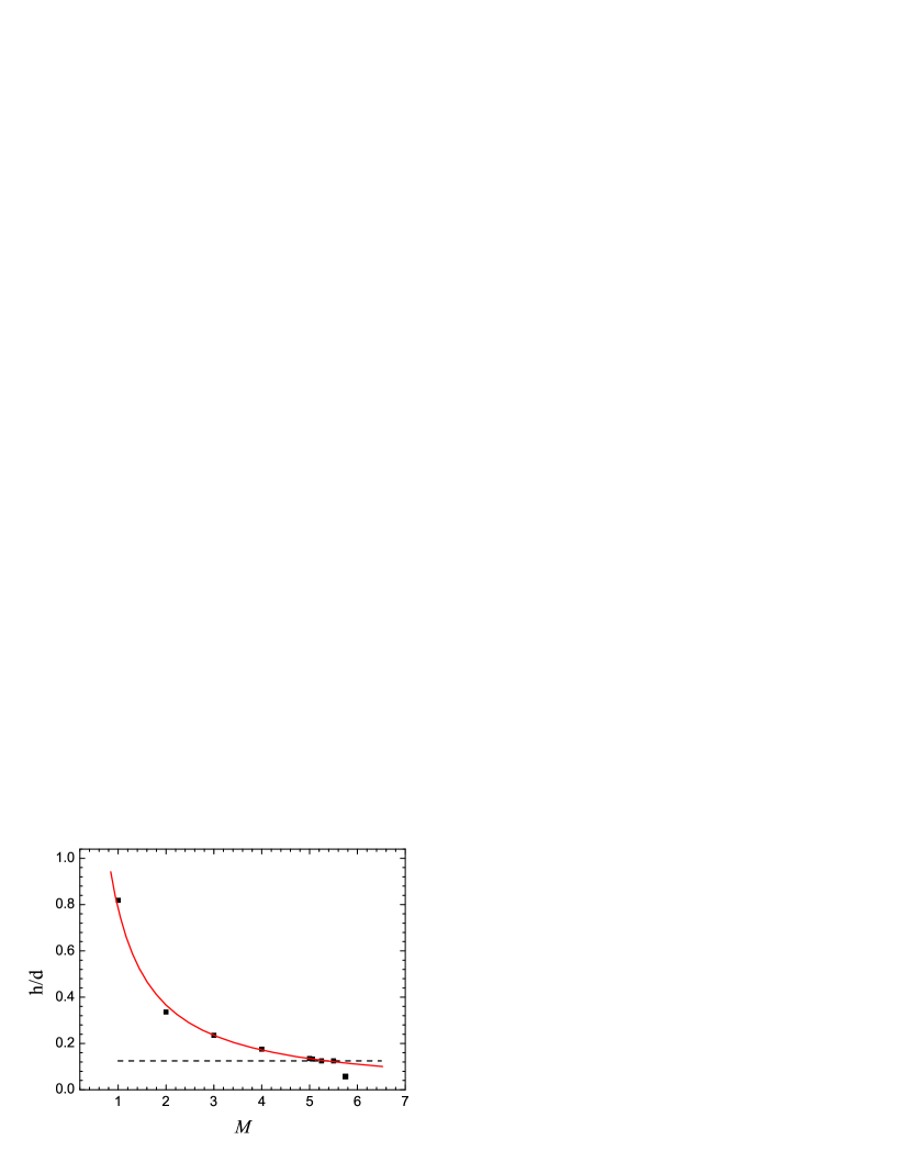
Figure 2: The final height of the flux ropes as a function of the relative dipole magnetic field strength $M$. Solid points indicate the final location of the flux rope. The dashed line denotes the initial hight of the flux rope at $h/d=0.125$. The red solid curve is a freehand interpolation of the numerical results, and it displays the power-law function $h/d=10^{-0.1}M^{-1.1}$, where $d$ is the depth of the background dipole field, and $M$ is a dimensionless parameter which gives the relative strength between the dipole and the filament current.

3.2 Evolution of the system with different background fields

In this section, we focus on the influence of the background field on the evolution of the magnetic system. First, in order to solve a few open questions in the work of Forbes (1990) and compare our results with his. We investigate the influence of the different $M$ on the evolution of the system. The cases 15-18 are presented with different $M$ given the same $d$, $h_{0}$ and $r_{0}$.

Figure 3 plots the height of the flux rope $h$ as a function of time in different $M$. When the background field is equal to zero ($M=0.0$), the initial repulsive force on the flux rope is large, and the flux rope promptly rises at the beginning. This agrees with the result in Forbes (1990). However, after about $t=2.0$ s, our flux rope’s trajectory differs from the result of Forbes (1990). Figure 8 of Forbes (1990) shows that at about $t=2.0$ s and $M=0.0$ the speed of flux rope becomes warped. However, this warp do not represent in our simulations. The reasons why we have different results are: 1) this increase could be a numerical artifact of the open boundary conditions; or 2) it is because of the lack of a gravitationally stratified solar atmosphere. In this present work, we used the same boundary conditions of Forbes (1990) and considered the gravitationally stratified background solar atmosphere. By comparison of our numerical simulations with Forbes (1990), we find that the warp of the height of flux rope may be eliminated by gravitational stratification effect. The flux rope when $M=1$ in the work of Forbes (1990) stops at some height after it rises up at the very start, and then moves downward slightly before continuing to rise further. Our results indicate that the gravitationally stratified medium can account for this phenomenon.

Figure 3: $h/d$ as a function of time. $h$ is the flux rope height. $d$ is the depth of the background dipole field. $M$ is a dimensionless parameter which gives the relative strength between the dipole and the filament current.

At the beginning of the experiment, the flux rope keep rising rapidly until the magnetic tension produced by the stretching of the line-tied field lines becomes large enough to slow down its upward motion. The Lorentz force $\mathbf{J}\times\mathbf{B}$ plays a main role in the decrease of the initially upward velocity of the flux rope. From Figure 3, we see that for $M=2$ the height of the flux rope remains almost constant after $t=500s$. It is because that the flux rope reaches the new equilibrium state at that time. By Equation (3) of Forbes 1990, we can further check whether the state of the flux rope is in equilibrium or not. We take the height of the flux rope $h$, the depth of the dipole $d$ and the relative strength of the dipole $M$ at $t=600$ s into Equation (3) of Forbes 1990, and find that the left almost equals the right of Equation (3). This means that the new equilibrium state is achieved.

Since the evolution of the system in the corona may be controlled by the background field, we need to investigate how the evolution of the magnetic system relies on the values of the background field strength, i.e. $m$. Figure 4 shows the height of the flux rope in the different background field strength $m$. The depth of the background dipole field and the initial current strength of the flux rope are $d=0.625\times 10^{4}$ km and $I_{0}=3\times 10^{11}$ A. The solid line corresponds to $m=0$, the dot curve is for $m=dI_{0}$ and the dashed curve for $m=2dI_{0}$. From Figure 4, we can see that the height of the flux rope becomes higher when the background field strength gets smaller. This implies that the flux rope can escape more easily following the catastrophe if the background field is weak.

Figure 4: $h/d$ as a function of time for the different background field $m$. $h$ is the height of the flux rope. $d=0.625\times 10^{4}$ km and $I_{0}=3\times 10^{11}$ A are the the depth of the background dipole field and the initial current strength of the flux rope. The solid line corresponds to $m=0$, the dot curve is for $m=dI_{0}$, and the dashed curve is for $m=2dI_{0}$. The lower panel is the zoom-out for time from 0 to 50 s.

To further demonstrate the relation between the strength of the background field and the flux rope, we studied the evolutions of the magnetic configuration in two cases in Figure 4. As shown in Figure 5, the magnetic field lines are represented by continuous contours. The left and right panels show $m=2dI_{0}$ and $m=dI_{0}$, and they correspond to the dashed, dot curves in Figure 4, respectively. From Figure 5, we can notice that the flux rope in the right panel is higher than in the left one. In addition, we are also able to recognize the existence of the X-point in these two panels, which may result in fast energy dissipation via magnetic reconnection.

Figure 5: Evolutions of the magnetic configuration at the different value of $m$ at $t=600$ s. The left and right panels show $m=2dI_{0}$ and $m=dI_{0}$. They correspond to the dashed and dot curves in Figure 4, respectively.

3.3 The internal evolution of the flux rope and effect of its radius

The flux rope moves upward very quickly driven by the unbalanced magnetic compression at the beginning of our simulation, whilst small perturbation on the amplitude of the flux rope along its radial direction always occurs since the initial state within the filament is never in exact equilibrium. Flow always appears within the filament almost at once as shown in Figure 6. The upper panel in this figure shows velocity streamlines at two different times for the stable equilibrium with $M=2.25$ (case 1), while the lower panel shows velocity streamlines for the nonequilibrium case with $M=1.0$ (case 2). The circle in each panel represents the position of the flux rope. At $t=1$ s, the flow speed for the stable case is about 0.8 the speed for the nonequilibrium case. Meanwhile, the flow speed at $t=2$ s for the stable equilibrium equals approximately the speed at $t=5$ s for the nonequilibrium. These results show that the internal flow of the flux rope remains small and does not last very long when the initial state of the flux rope commences from the stable branch of the theoretical equilibrium curve.

Figure 6: Velocity streamlines at two different times for the stable equilibrium with $M=2.25$ (case 1) in (a) and (b), and the nonequilibrium case with $M=1.0$ (case 2) in (c) and (d). The circles indicate the position of the flux rope.

In order to understand the influence of the computational domain on the internal evolution of the flux rope, we also investigate the internal evolution of the flux rope in two different computational domains. Figure 7 shows evolution of the height of the flux rope with respect to time for the stable equilibrium with $M=2.25$ (case 1) in the two computational domains [$(-4L,4L)\times(0,8L)$ in (a) and $(-L,L)\times(0,2L)$ in (b)] with the same grid points $800\times 800$. The solid curves are evolution of the height of the flux rope with respect to time for case 1, and the dashed lines correspond to the initial height $h_{0}=0.0625\times 10^{5}$ km for case 1. We can see that the readjustment of the height of the flux rope accomplished by $t=2$ s in (a). After 2 s, the flux rope remains stationary at the height about $0.06\times 10^{5}$ km. However, after taking $t=3$ s in (b), it becomes stationary at the height about $\sim 0.0625\times 10^{5}$ km.

The information revealed by Figure 7 suggests that the numerical diffusion is faster when the computational domain is larger. Whereas, the numerical error is larger in (a) than (b), since the numerical error can be estimated by the ratio of the grid spacing to the initial height $\bigtriangleup x/h_{0}$, i.e. 16% in (a) and 4% in (b). Because of the numerical error, the stationary height of the flux rope is closer to the initial height in (b) than in (a).

Figure 7: The flux rope height $h$ as a function of time for the same stable equilibrium (case 1) in the different computational domain with the same grid points: the left panel represents $(-4L,4L)\times(0,8L)$ with $800\times 800$ grid points, and the right panel depicts $(-L,L)\times(0,2L)$ with $800\times 800$ grid points. The solid curves are for case 1, and the dashed lines correspond to the initial height $h_{0}=0.0625\times 10^{5}$ km for case 1.

In order to investigate the influence of the radius of flux rope on its evolution, we have performed two simulations (cases 3 and 4). We vary the radius of the flux rope in these two cases, while other parameters remain unchanged. The values of the parameters are listed in Table 2. Figure 8 displays evolution of the height of flux rope with respect to time in these cases. Curve $r_{0}=3000$ km is for case 3, while curve $r_{0}=5000$ km is for case 4. From this figure, we see that the flux rope with larger radius apparently has faster upward velocity than that with smaller radius, which means that greater radii can result in eruption of flux rope more easily.

Figure 8: Variation of the flux rope height versus time for cases 3 and 4: curves $r_{0}=3000$ km is for case 3, and curve $r_{0}=5000$ km is for case 4. $d$ is the depth of the background dipole field and it is same for these two cases.

4 Discussions and Conclusions

We numerically investigate the evolution of the flux rope using the ZEUS-2D code for modelling the prominence or the filament in the corona, which may eventually erupt as catastrophe. The empirical S&G atmosphere model is employed for the distribution of the density of the background field. Our present simulations has a higher resolution than the previous work, e.g. Wang et al. (2009) and Forbes (1990), due to the larger simulation domain and more grid points. We studied the influence of the strength of the background field and the radius of the flux ropes on the internal, overall equilibrium and escape of the flux ropes in the detailed simulations, including $18$ cases for the different combinations of several important parameters. The main conclusions are drawn as follows.

1. In our simulations, by using the realistic plasma environment and much higher resolution, we notice some different characters compared to previous studies in Forbes (1990). We find that the speed of the flux rope do not become warped after $t=2.0$ s for $M=0$ and for $M=1$ ($M$ is the ratio of the strength of the dipole field $m$ and the product of the filament current $I$ and the depth $d$ of the dipole field, i.e. $M=m/(Id)$), which differs from the results in Forbes (1990). The flux rope would rather keep rising slowly, and stop at some height after some time, then moves downwards slightly before continuing to rise further.

2. Among cases 4-12, the final height of the flux rope varies with $M$ (the ratio of the strength of the dipole field $m$ and the product of the filament current $I$ and the depth $d$ of the dipole field, i.e. $M=m/(Id)$) in the way of power-law function $h/d=10^{-0.1}M^{-1.1}$.

3. The flux rope can escape more easily if the background magnetic field is weaker. This implies that the catastrophe behavior can be triggered by suppressing the strength of the background magnetic field, which is consistent with previous work by Forbes (1990), Isenberg et al. (1993), Lin et al. (1998, 2007), Chen (2011). The decay of the photospheric magnetic field due to the magnetic diffusion may result in the eruption of the flux rope (Mackay & van Ballegooijen 2006), and further explain why the peak rate of the CME occurrence is usually delayed by $6-12$ months with respect to the peak of the Sunspot number (Robbrecht et al. 2009).

4. The initial radius of the flux rope may have significant influence on its evolution. The results indicate that the flux rope with larger initial radius erupts more easily.

5. The internal flow of the flux rope remains small and does not last very long when the initial state of the flux rope commences from the stable branch of the theoretical equilibrium curve. We also find that the time and velocity of this flow are related to the computational domain. Provided that the grid points remain unchanged, the increase of the computational domain can result in shorter time for the internal equilibrium of the flux rope, whilst the numerical error is in an expected range.

The authors appreciate C. Shen and Z. Mei for valuable discussions on the techniques of numerical simulation. They are also grateful to the referee for valuable comments and suggestions that improved this paper. This work was supported by the National Basic Research Program of China (2012CB825600 and 2011CB811406), and the Shan-dong Province Natural Science Foundation (ZR2012AQ016). JL’s work was supported by the Program 973 grants 2011CB811403 and 2013CBA01503, the NSFC grants 11273055 and 11333007, and the CAS grants KJCX2-EW-T07 and XDB09040202.

References

- [2002] Chen, P. F., Wu, S. T., Shibata, K., & Fang, C. 2002, ”Evidence of EIT and Moreton Waves in Numerical Simulations”, ApJ, 572, L99
- [2011] Chen, P. F. 2011, ”Coronal Mass Ejections: Models and Their Observational Basis”, Living Rev. Solar Phys., 8, lrsp-2011-1. URL
- [2000] Forbes, T. G. 2000, ”A review on the genesis of coronal mass ejections”, J. Geophys. Res., 105, 23153-23166
- [1990] Forbes, T. G. 1990, J. Geophys. Res., 95, 11919
- [1991] Forbes, T. G., & Isenberg, P. A. 1991, ApJ, 373, 294
- [1995] Forbes, T. G., & Priest, E. R. 1995, Photospheric magnetic field evolution and eruptive flares, ApJ, 446, 377-389
- [1993] Isenberg, P. A., Forbes, T. G., & Demoulin, P. 1993, ApJ, 417, 368
- [2013] Kliem, B., Su, Y. N., van Ballegooijen, A. A. & Deluca, E. E. 2013, ApJ, 779, 129
- [2012] Kusano, K., Bamba, Y., Yamamoto, T. T., Iida, Y., Toriumi, S. & Asai, A. 2012, ApJ, 760, 31
- [1998] Leblanc, Y., Dulk, G. A., & Bougeret, J.-L. 1998, Solar Phys., 183, 165
- [2013] Li, L. P., & Zhang, J. 2013, A & A, 552L, 11L
- [1998] Lin, J., Isenberg, P. A., & Demoulin, P. 1998, ApJ, 504, 1006
- [2007] Lin, J. 2007, ChJAA, 7, 457
- [2000] Lin, J., & Forbes, T. G. 2000, J. Geophys. Res., 105, 2375
- [2002] Lin, J. 2002, ChJAA, 2, 539
- [2006] Lin, J., Mancuso, S., & Vourlidas, A. 2006, ApJ, 649, 1110
- [2006] Mackay, D. H., & van Ballegooijen, A. A. 2006, ApJ, 641, 577
- [2012] Mei, Z. X., Udo, Z., & Lin, J. 2012a, ScChG, 55, 1316M
- [2012] Mei, Z. X., Shen, C., Wu, N., Lin, J., Murphy, N. A., & Roussev, I. I. 2012b, MNRAS, 425, 2824
- [2007] Pulkkinen, T. 2007, ”Space Weather: Terrestrial Perspective”, Living Rev. Solar Phys., 4, lrsp-2007-1. URL
- [2009] Robbrecht, E., Berghmans, D., & Van der Linden, R.A.M. 2009, ApJ, 691, 1222
- [2006] Schwenn, R. 2006, ”Space Weather: The Solar Perspective”, Living Rev. Solar Phys., 3, lrsp-2006-2. URL
- [2013] Shen, C. C., Reeves, K. K., Raymond, J. C., Murphy, N. A., Ko, Y.-K., Lin, J., Mikic, Z. & Linker, J. A. 2013, ApJ, 773, 110
- [1999] Sittler, E. C., & Guhathakurta, M. 1999, ApJ, 523, 812
- [1992] Stone, J. M., & Norman, M. L. 1992a, ApJS, 80, 753
- [1992] Stone, J. M., & Norman, M. L. 1992b, ApJS, 80, 791
- [1992] Stone, J. M., Mihalas, D., & Norman, M. L. 1992c, ApJS, 80, 819
- [2009] Wang, H., Shen, C., & Lin, J. 2009, ApJ, 700, 1716
- [2011] Welsch, B. T., Christe, S., & McTiernan, J. M. 2009, ApJ, 700, 1716
- [2012] Yu, C., 2012, ApJ, 757, 67
- [2011] Zhang, Y. Z., Feng, X. S., & Song, W. B. 2011, ApJ, 728, 21