Optical knots and contact geometry II.

From Ranada dyons to transverse and

cosmetic knots

Arkady L. Kholodenko 

375 H.L.Hunter Laboratories, Clemson University, Clemson, SC 29634-0973,USA

Abstract

Some time ago Ranada (1989) obtained new nontrivial solutions of the Maxwellian gauge fields without sources. These were reinterpreted  in  Kholodenko (2015a) (part I) as particle-like (monopoles, dyons, etc.). They were obtained by the method of Abelian reduction of the non-Abelian Yang-Mills functional. The developed method uses  instanton-type calculations normally employed for the non-Abelian gauge fields. By invoking the electric-magnetic duality it then becomes possible to replace all known charges/masses by the particle -like solutions of the source-free Abelian gauge fields. To employ these results in high energy physics, it is essential to to extend Ranada’s results by carefully analysing and classifying all  dynamically generated knoted/linked structures in gauge fields, including those discovered by Ranada. This task is completed in this work. The study is facilitated by the recent progress made in solving the Moffatt conjecture. Its essence is stated as follows: in steady incompressible Euler-type fluids the streamlines could have knots/links of all types. By employing  the correspondence between the ideal hydrodynamics and electrodynamics discussed in part I and by superimposing it with the already mentioned method of Abelian reduction, it is demonstrated that in the absence of boundaries only the iterated torus knots and links could be dynamically generated. Obtained results allow to develop further particle-knot/link correspondence studied in Kholodenko (2015b)

Keywords:

Contact geometry and topology

Knot theory

Morse-Smale dynamical flows

Hydrodynamics

1. Introduction

The existence-type proofs [$1,2$] of Moffatt conjecture [$3$] are opening Pandora’s box of all kinds of puzzles. Indeed, from the seminal work by Witten [$4$] (see also Atiyah [$5$]) it is known that the observables for both the Abelian and non Abelian source-free gauge fields are knotted Wilson loops. It is believed that only the non Abelian  Chern-Simons (C-S) topological field theory is capable of detecting nontrivial knots/links.  By ”nontrivial knots” we mean knots other than unknots, Hopf links and torus-type knots/links. Being topological in nature the C-S  functional is not capable of taking into account boundary conditions. This is true for all known to us path integral treatments of the Abelian  and non-Abelian C-S  field theories. In the meantime the boundary conditions do play an important role in  the work by Enciso and Peralta -Salas [$1$] on solving the Moffatt conjecture. This conjecture can be formuated as follows: in steady incompressible Euler-type fluids the streamlines could have knots/links of all types. The correspondence between hydrodynamics and Maxwellian electrodynamics discussed in our book $[6]$ makes results of [$1$] transferable to the Abelian/Maxwellian electrodynamics where, in view of this correspondence it is possible, in principle, to generate knots/links of all types. The fact that the Abelian gauge fields are capable of producing the nontrivial knots/links blurs the barriers between the Maxwellian electrodynamics, Yang-Mills fields and gravity. As result, recently, there has been (apparently uncorrelated) visibly large activity in electromagnetism [$7$], non Abelian gauge fields [$8$], and gravity [$9$] producing torus-type knots/links by using more or less the same methods. Although the cited papers are presented as the most recent and representative ones, there are many other papers describing the same type of knotty structures in these fields. Also, in the magnetohydrodynamics, in condensed matter physics, etc. Unlike other treatments,  here we are interested in study and clssification of all possible knots/links which can be dynamically generated.

From knot theory and, now proven, geometrization conjecture it follows that complements of knots/links embedded in $S^{3}$ are spaces of positive, negative and zero curvature. Thus far the ability to curve the ambient space was always associated with physical masses. With exception of neutrinos, the Higgs boson is believed to supply physical masses to the rest of particles. Now we encounter a situation when the space is being curved by knots/links produced by stable (on some time scales) configurations of gauge fields of both Abelian and non Abelian nature. In part I [$10$] (Kholodenko 2015a))  and in our book [$6$] we argued that the electric and magnetic charges can be recreated by the Hopf-like links of the respective gauge fields. Surely, such charges must also be massive. If such massive particle-like formations are created by the pure gauge fields then, apparently, all known elementary masses and charges  can be topologically described. Attempts to do so is described  in a number of publications, begining with paper by Misner and Wheeler [$11$] and Atiyah at all [$12$], and ending with our latest paper [$13$] (Kholodenko 2015b). Just mentioned replacement has many advantages. In particular, if one believes that the non-Abelian gauge fields are just natural generalizations of more familiar Maxwellian fields, then one encounters a problem of existence of non-Abelian charges-analogs of (seemingly) familiar charges in Maxwell’s electrodynamics. Surprisingly, to introduce the macroscopic charges  into non-Abelian fields is a challenging task which, to our knowledge, is not completed. By treating gravity as gauge theory, the analogous problem exists in gravity too. In gravity it is known as the problem of description of dynamics of extended bodies. The difficulties in description of extended objects in both the Y-M and gravity fields  are summarized on page 97 of our book [$6]$.

This work is made of seven sections and seven appendices. Almost book-style manner of presentation in this paper is aimed at making it accessible for readers with various backgrounds: from purely physical to purely mathematical. As in part I [$10$], for a quick introduction to ideas and methods of contact geometry/topology our readers may consult either [$6$], aimed mainly at readers with physics background, or [$14$] aimed at mathematicians.

In section 2 we provide the statement of the problem to be studied written in the traditional style of boundary value type problem. In the same section we reformulate our problem in the language of contact geometry. In section 3 we introduce the Reeb and the Liouville vector fields and compare them with the Beltrami vector field playing central role in both Part I and in this work. Section 4 is essential for the whole paper. In it we establish the chain of correspondences: Beltrami vector fields $\iff$Reeb vector fields$\iff$Hamiltonian vector fields. These correspondences allow us to introduce the nonsingular Morse-Smale (NMS) flows.  In section 5 we connect these flows with the Hamiltonian flows discussed (independently of NMS flows) by Zung and Fomenko [$15$]. In section 6 we explicitly derive the iterated torus knot structures predicted by Zung and Fomenko in their paper [$15$] of 1990. These structures are obtained via cascade of bifurcations of Hamiltonian vector fields which we describe in some detail. In the absence of boundaries, these are the only knotted linked structures which can be dynamically generated. We also reinterpret the obtained iterated torus knots/links in terms of the transversely simple knots/links known in contact geometry/topology. As a by product, we introduce the Legendrian and transverse knots  and links. Since the Legendrian knots/links  were christened by Arnol’d as optical knots/links we use this terminology in the titles of both parts I and II of our work. In section 7 we relate results of Birman and Williams papers [$16,17$] with what was obtained already in previous sections in order to obtain other knots and links of arbitrary complexity. These are obtainable only in the presence of boundaries. Along this way we developed new method of designing the Lorenz template. This template was  originally introduced in Birman and Williams paper [$16$] in order to facilitate the description of closed orbits occuring in dynamics of Lorenz equations. The simplicity of our derivation of this template enabled us to reobtain the universal template of Ghrist [$18$] by methods different from those by Ghrist.  Possible applications of the obtained results to gravity are discussed in section 7 in the context of cosmetic (not cosmic!) knots. Appendices- from A to G -contain all kinds of support information needed for uninterrupted reading of the main text.

2.  Force-free/Beltrami equation from the point of view of contact geometry

From Theorem 4.1. [$10$] (part I) it follows that force-free/Beltrami  vector fields are solutions of the steady Euler flows. At the same time, Corollary 4.2. is telling us that such flows minimize the kinetic energy functional. This is achieved due to the fact that Beltrami/force-free fields have nonzero helicity. The helicity is playing the central role in Ranada’s papers [$19,20$]. By studying helicity Ranada discovered his torus-type knots/links. The same type of knots were recently reported by Kedia et al  [$21$]. Based on results of part I, it should be obvious that study of helicity is synonymous with the study of knots and links (at least of torus-type). Can the same be achieved by studying the Beltrami/force-free equation? We would like to demonstrate that this is indeed possible. Although the literature on solving the Beltrami equation is large, only quite recently the conclusive results on existence of knots and links in Belrami flows have been published. An example of systematic treatment of Beltrami flows using conventional methods of  partial differential equations is given in the pedagogically written monograph by Majda and Bertozzi [$22$]. Our readers should be aware of many other examples existing in literature. All these efforts culminated in  the Annals of Mathematics paper by Enciso and Peralta-Salas [$1$]. In this paper the authors proved that the equation for (strong) Beltrami fields

$$\mathbf{\nabla}\times\mathbf{v}=\kappa\mathbf{v}$$ (2.1a)

(that is  the Beltrami equation with constant $\kappa)$ supplemented with the boundary condition

$$\mathbf{v\mid}_{\Sigma}=\mathbf{w}$$ (2.1b)

,where $\Sigma$ is embedded oriented analytic surface  in $\mathbf{R}^{3}$ so that  the vector $\mathbf{w}$ is tangent to $\Sigma,$ can have solutions  describing knots/links of any type (that is not just torus knots/links). Subsequent studies by the same authors [$23$] demonstrated that $\Sigma$ is actually having a toral shape/topology. These authors were able to prove what Moffatt proposed/conjectured long before heuristically [$3$].The same conclusion was reached in 2000,  by Etnyre and Ghrist [$2$] who were using methods of contact geometry and topology. Both Enciso and Peralta-Salas and Etnyre and Ghrist presented a sort of existence-type proof of the Moffatt conjecture.

In this paper we present yet another proof (constructive) of Moffatt’s conjecture. It is based on methods of contact geometry and topology. Our results can be considered as some elaboration on the results by Etnyre and Ghrist [$2$]. Unlike the existence-type results of previous authors, we were able to find explicitly some of the knots/links being guided (to some extent) by the seminal works by Birman and Williams [$16,17$], Fomenko [$24$] and Ghys [$25$]. It is appropriate to mention at this point that recently proposed experimental methods of generating knots and links in fluids [$26$] are compatible with those discussed by Birman and Williams [$16,17$], Ghys [25] and Enciso and Peralta -Salas [$1$]. Following Etnyre and Ghrist [$27$] we begin our derivation by rewriting the Beltrami eq.(2.1a) as

$$\ast d\alpha=\kappa\alpha,$$ (2.2a)

where $\alpha$ is any contact 1-form and $\ast$ is the Hodge star operator. Although details of derivation of eq.(2.2a) are given in Chr.5 of  [$6$], for physics educated readers basics are outlined in the Appendix A. Since $\ast\ast=id$ , the same equation can be equivalently rewritten as

$$d\alpha=\kappa\ast\alpha.$$ (2.2b)

Should $\kappa=1,$ the above equation would coincide with the standard Hodge relation between 1 and 2 forms. Following Etnyre and Ghrist [$27$] we need the following

Definition 2.1. The Beltrami field is called rotational if $\kappa\neq 0.$

For this case, we can introduce the volume 3-form $\mu$ as follows

$$\mu=\alpha\wedge d\alpha=\kappa\alpha\wedge\ast\alpha=\kappa dV.$$ (2.3a)

The volume form $\kappa dV$ can be re normalized so that the factor (function) $\kappa$ can be eliminated. This is so because the volume form $dV$contains the metric factor $\sqrt{g}$ which can be readjusted. This fact can be formulated as

Theorem 2.2. (Chern and Hamilton [$28$]) Every contact form $\alpha$ on a 3-manifold has the adapted Riemannian metric $g.$

The metric is adapted (that is normalized) if eq.(2.2b)  can be replaced by

$$d\alpha=\ast\alpha$$ (2.2.c)

This result can be recognized as the standard result from the Hodge theory. For such a case we obtain:

$$\mu=\alpha\wedge\ast\alpha=dV.$$ (2.3b)

Consider now the volume integral

$$I=\mathop{\displaystyle\int}\limits_{Y}\alpha\wedge\ast\alpha.$$ (2.4)

On one hand, it can be looked upon as the action functional for the 3d version of the Abelian/Maxwellian gauge field theory as discussed in Sections 2 and 3 of part I, on another, the same functional can be used for description of dynamics of 3+1 Einsteinian gravity  [$29,30$]. In view of  Theorem 2.2., eq.(2.2c) can be rephrased now as

Corollary 2.3. Every 3-manifold admits a non-singular Beltrami flow for some Riemannian structure on it. That is to say, study of the Beltrami fields on 3-manifolds is equivalent to study of the Hodge theory on 3-manifolds.

The non singularity of flows is assured by the requirement $\kappa\neq 0.$ The above statement does not include any mention about the existence of knots/links in the Beltrami flows. Thus, the obtained results are helpful but not constructive yet. To obtain constructive results we need to introduce the Reeb vector fields associated with contact structures. For our purposes it is sufficient to design the Reeb vector fields only for $S^{3}$.

3.    Reeb vs Beltami vector fields on $S^{3}\vskip 12.0pt plus 4.0pt minus 4.0pt$

Following Geiges [$14$] we begin with the definition of the Liouville vector field X. For this purpose we need to use the symplectic 2-form introduced in (4.15a) of part I defined on R${}^{4}.$ Up to a constant factor it is given by

$$\omega=dx_{1}\wedge dy_{1}+dx_{2}\wedge dy_{2}.$$ (3.1)

If we use the definition of the Lie derivative $\mathcal{L}_{X}$ for the vector field $\mathbf{X}$

$$\mathcal{L}_{X}=d\circ i_{X}+i_{X}\circ d,$$ (3.2)

then, we arrvie at the following

Definition 3.1.  The vector field $X$ is called Liouville if it obeys the equation

$$\mathcal{L}_{{}_{X}}\omega=\omega.$$ (3.3)

The contact 1-form $\alpha$ can be defined now as

$$\alpha=i_{X}\omega.$$ (3.4)

This formula connects the symplectic and contact geometries in the most efficient way. To find the Liouville vector field $\mathbf{X}$ for $S^{3}$ we notice that eq.(3.3) may hold for any form and, therefore, such a form could be, say, some function $\mathfrak{f}$. In this case eq.(3.3) acquires the form  [$31$]

$$\mathop{\displaystyle\sum}\limits_{i}x_{i}\frac{\partial\mathfrak{f}}{\partial x_{i}}=\mathfrak{f}.$$

Using this result, the Liouville vector field $\mathbf{X}$ on $S^{3}$, where $S^{3}$ is defined by the equation $r^{2}=x_{1}^{2}+y_{1}^{2}+x_{2}^{2}+y_{2}^{2},$ is given by

$$\mathbf{X}=\frac{1}{2}(x_{1}\partial_{x_{1}}+y_{1}\partial_{y_{1}}+x_{2}\partial_{x_{2}}+y_{2}\partial_{y_{2}}).$$ (3.5)

To check correctness of this result, by combining eq.s(3.4)-(3.5) and using properly normalized eq.(4.14) of part I, we obtain

$$\mathcal{L}_{{}_{X}}\omega=d\circ i_{X}\omega=d\circ\alpha=d[\frac{1}{2}\mathop{\displaystyle\sum}\nolimits_{i=1}^{2}(x_{i}dy_{i}-y_{i}dx_{i})]=\omega$$ (3.6)

as required. Going back to eq.(3.4) we would like to demonstrate now that the 1-form $\alpha$ can be also obtained differently. This is so because the very same manifold has both the symplectic and the Riemannian structure. In the last case the metric 2-form $g=g_{ij}dx^{i}\otimes dx^{j}$ should be defined. Then, for the vector field $\bar{X}=X^{i}\frac{\partial}{\partial x^{i}}$ we obtain (using definitions from Appendix A): $\bar{X}^{b}$ $=i_{\bar{X}}g=g(\bar{X},\cdot)\equiv g_{ij}X^{i}dx^{j}$. From the same appendix we know that if the operator $\flat$ transforms vector fields into 1-forms, then the inverse operator $\natural$ is transforming 1-forms into vector fields, that is $[X^{\flat}]^{\natural}=g^{ij}X_{i}\frac{\partial}{\partial x^{j}}=X^{i}\frac{\partial}{\partial x^{i}}=\bar{X}.$ Suppose now that $\alpha=\tilde{X}^{b}=i_{\tilde{X}}g$ for some vector field X̃ such that $\alpha=\tilde{X}^{b}=i_{\tilde{X}}g=i_{X}\omega.$ This can be accomplished as follows. Suppose that X̃ is the desired  vector field then, we can normalize it as

$$i_{\tilde{X}}\alpha=i_{\tilde{X}}i_{\tilde{X}}g=1.$$ (3.7)

Explicitly, this equation reads $i_{\tilde{X}}[g_{ij}\tilde{X}^{i}dx^{j}]=g_{ij}\tilde{X}^{i}\tilde{X}^{j}=1.$ This result is surely making sense. Furthermore, the above condition can be safely replaced by $g_{ij}\tilde{X}^{i}\tilde{X}^{j}>0$. This is so, because in the case of $S^{3}$ the condition given by eq.(3.7) reads: $x_{1}^{2}+y_{1}^{2}+x_{2}^{2}+y_{2}^{2}=1.$ Therefore, it is clear that this condition can be relaxed to $x_{1}^{2}+y_{1}^{2}+x_{2}^{2}+y_{2}^{2}=r^{2}$ $>0.$ The condition, eq.(3.7), is the 1st of two conditions defining the Reeb vector field.  The 2nd condition is given by

$$i_{\tilde{X}}d\alpha=0.$$ (3.8)

Suppose that, indeed, $\alpha=i_{\tilde{X}}g=i_{X}\omega,$ where $X$ is the Liouville and $\tilde{X}$ is the Reeb vector field. Then, we have to require: $i_{\tilde{X}}d\alpha=i_{\tilde{X}}d\circ i_{\tilde{X}}g=i_{\tilde{X}}d\circ i_{X}\omega=i_{\tilde{X}}\omega=0$. This requirement allows us to determine the Reeb field.  It also can be understood physically. For this purpose we consider the volume 3-form $\ \mu=\alpha\wedge d\alpha$ and apply to it the Lie derivative, i.e.

This result is obtained after we used  the  two Reeb conditions. Clearly, for the Reeb fields the equation

$$\mathcal{L}_{{}_{\tilde{X}}}\mu=0$$ (3.10)

is equivalent to the incompressibility condition for fluids, or to the transversality condition div$\mathbf{A}=0$ for electromagnetic fields.

From here we obtain the major

Corollary 3.2. From eq.(3.9) it follows that the condition  $\mathcal{L}_{{}_{\tilde{X}}}\alpha=0$ is implying that the Reeb vector field  flow preserves the form $\alpha$ and, with it, the contact structure $\xi=\mathit{ker}$ $\alpha.\vskip 12.0pt plus 4.0pt minus 4.0pt$ $\ Alternatively,$ the Reeb vector field $\tilde{X}$ is determined by the condition $\mathcal{L}_{{}_{\tilde{X}}}\alpha=0.\vskip 12.0pt plus 4.0pt minus 4.0pt$

Nevertheless, we would like to demonstrate now that the condition $i_{\tilde{X}}\omega=0$ is also sufficient for determination of the Reeb field.  For the tasks we are having in mind, it is sufficient to check this condition for $S^{3}$ where the results are known  [$6,14$]. Specifically, it is known that for $S^{3}$ the Reeb vector field is given by

$$\tilde{X}=2(x_{1}\frac{\partial}{\partial y_{1}}-y_{1}\frac{\partial}{\partial x_{1}}+x_{2}\frac{\partial}{\partial y_{2}}-y_{2}\frac{\partial}{\partial x_{2}}).$$ (3.11)

By combining eq.s(3.1) and (3.11) we obtain:

$$i_{\tilde{X}}\omega=-2(x_{1}dx_{1}+y_{1}dy_{1}+x_{2}dx_{2}+y_{2}dy_{2}).$$ (3.12)

However, in view of the fact that $x_{1}^{2}+y_{1}^{2}+x_{2}^{2}+y_{2}^{2}=r^{2},$ we obtain as well: $2rdr=2\left(x_{1}dx_{1}+y_{1}dy_{1}+x_{2}dx_{2}+y_{2}dy_{2}\right)=0,$ if this result is to be restricted to $S^{3}.$ Thus, at least for the case of $S^{3},$ we just have obtained $i_{\tilde{X}}\omega=0$ as required.

Eq.(3.4), when combined with eq.(3.5), yields $\alpha=i_{X}\omega=\frac{1}{2}\{eq.(4.14),$part I} in accord with eq.(3.6). Now we take again $\alpha=\tilde{X}^{b}=i_{\tilde{X}}g=i_{X}\omega$ and, since $\tilde{X}^{b}=g_{ij}\tilde{X}^{i}dx^{j},$ we obtain

$$\alpha=\tilde{X}^{b}=g_{ij}\tilde{X}^{i}dx^{j}.$$ (3.13)

By combining eq.s(3.11) and (3.13) we again recover $\alpha=i_{\tilde{X}}g=\frac{1}{2}\{eq.(4.14),$part I$\}.$ Therefore, we just demonstrated that, indeed, $i_{\tilde{X}}g=i_{X}\omega,$ where $\tilde{X}$ is the Reeb and $X$ is the Liouville vector fields. By combining eq.(3.13) with eq.(A.5) and (2.2a) we re obtain now the Beltrami equation

$$\ast d\tilde{X}^{\flat}=\kappa\tilde{X}^{b}.$$ (3.14)

Clearly, it is equivalent to either eq.(2.2a) or (2.2b). Furthermore, in view of the Theorem 2.2., it is permissible to put $\kappa=1.$

Next, suppose that $\ast\alpha=i_{\tilde{X}}\mu$ then, for the r.h.s  of this equality we obtain: $i_{\tilde{X}}\mu=\left(i_{\tilde{X}}\alpha\right)\wedge d\alpha-\alpha\wedge i_{\tilde{X}}d\alpha=d\alpha.$ This result becomes possible in view of the 1st and 2nd Reeb conditions. Thus, we just reobtained eq.(2.2c). The obtained results can be formulated as

theorem.  It is of major importance  for this work

Theorem 3.3. Any rotational Beltrami field on a Riemannian 3-manifold is Reeb-like and vice versa

Corollary 3.4. Every Reeb-like vector field generates a non-singular steady solution to the Euler equations for a perfect incompressible fluid with respect to some Riemannian structure. Equivalently, every Reeb-like vector field  which is solution of the force-free equation generates non-singular solution of the source-free Maxwell equations with respect to some Riemannian structure.

Appendix B provides an illustration of the Corollary 3.4. in terms of conventional terminology used in physics literature.

4.     Hamiltonian dynamics  and Reeb vector fields

Eq.(9.1a) of part I describes the conformation of the single vortex tube.  In view of the Beltrami condition, this equation can be equivalently rewritten as

$$[v_{x}\frac{\partial}{\partial x}+v_{y}\frac{\partial}{\partial y}+v_{z}\frac{\partial}{\partial z}]f=0.$$ (4.1a)

If we add just one (compactification) point to R³ we can use the stereographic projection allowing us to replace R³ by $S^{3}$ and to consider the conformation of the vortex tube in $S^{3}.$ Example 1.9. (page 123) from the book by Arnol’d and Khesin [$32$] is telling us (without proof) that the components of the vector $\mathbf{v}$ on $S^{3}$ are $\mathbf{v}=[x_{1},-y_{1},x_{2},-y_{2}].$  The same source (again without proof) is also telling us that the vector v is the eigenvector of the force-free equation curl${}^{-1}\mathbf{v}=\lambda\mathbf{v}$ with the eigenvalue $\lambda=1/2.$

In view of these results and using eq.(3.11) for the Reeb vector field, we replace eq.(4.1a) by

$$(x_{1}\frac{\partial}{\partial y_{1}}-y_{1}\frac{\partial}{\partial x_{1}}+x_{2}\frac{\partial}{\partial y_{2}}-y_{2}\frac{\partial}{\partial x_{2}})f=0$$ (4.1b)

Now, in view of eq.(9.1b)  of part I this equation can be equivalently rewritten as

$$\frac{dy_{1}}{x_{1}}=\frac{dx_{1}}{-y_{1}}=\frac{dy_{2}}{x_{2}}=\frac{dx_{2}}{-y_{2}}=dt$$ (4.1c)

so that we recover  the result of Arnol’d and Khesin for v. In addition, we obtain:

$$\dot{x}_{1} = -y_{1};\dot{x}_{2}=-y_{2}\TCItag{4.2}$$ (2)

$$\dot{y}_{1} = x_{1};\text{ \ \ }\dot{y}_{2}=x_{2}.$$

These are the Hamiltonian-type equations describing dynamics of two uncoupled harmonic oscillators. From mechanics it is known that all integrable systems can be reduced by a sequence of canonical transformations to the set of independent harmonic oscillators. The simplicity of the final result is misleading though as can be seen from the encyclopedic book by Fomenko and Bolsinov [$33$]. It is misleading because the dynamical system described by eq.s (4.2) possesses several integrals of motion. In particular, it has the energy $h=\frac{1}{2}(p_{1}^{2}+p_{2}^{2}+y_{1}^{2}+y_{2}^{2}),$where $p_{1}=x_{1},p_{2}=x_{2},$ as one of such integrals. The existence of $h$ indicates that the motion is constrained to $S^{3}.$ Thus, the problem emerges of classification of all exactly integrable systems whose dynamics is constrained to $S^{3}$. Surprisingly, there are many dynamical systems fitting such a classification. The full catalog is given  in the book by Fomenko and Bolsinov. Whatever these systems might be, once their description is reduced to the set of eq.s(4.2) supplemented by, say, the constraint of moving on $S^{3},$ their treatment follows the standard protocol. The protocol can be implemented either by the methods of symplectic mechanics [$31,34$] or by the methods of sub-Riemannian geometry-a discipline which is part of contact geometry  [$6,35$]. The results of, say, symplectic treatment indicate that the trajectories of the dynamical system described by eq.s(4.2) are the linked (Hopf) rings. This result is consistent with results of Ranada discissed in Part I. Furthermore, the same eq.s(4.1b) were obtained by Kamchatnov [$36$] whose analysis of these equations demonstrates that, indeed, in accord with the result by Arnol’d and Khesin [$32$], the largest eigenvalue $\lambda$ of  the Beltrami equation curl${}^{-1}\mathbf{v}=\lambda\mathbf{v}$ is $\frac{1}{2}$.  This result follows from eq.(16) of Kamchatnov’s paper where one should replace $x^{2}$ by 1 as required for description of a sphere $S^{3}$ of unit radius. The Example 1.9. in the book by Arnol’d and Khesin exhausts all possibilities available without further use of methods of contact geometry and topology.  These methods are needed, nevertheless, if we are interested in obtaining solutions of Hamiltonian eq.s(4.2) more complicated than Hopfian rings.

To begin  our  study of this topic, we would like to use the notion of contactomorphism defined by eq.(4.9) of part I. Now we are interested in applying it to the standard contact form on $S^{3}.$ To do so, we introduce the complex numbers $z_{1}=r_{1}\exp\{i\phi_{1}\}$ and $z_{2}=r_{2}\exp\{i\phi_{2}\}$ so that in terms of these variables the 3-sphere $S^{3}$ is described by the equation $r_{1}^{2}+r_{2}^{2}=1.$ The 1-form, eq.(4.14) of part I, can be rewritten in terms of just introduced variables as

$$\alpha=\frac{1}{2}(r_{1}^{2}d\phi_{1}+r_{2}^{2}d\phi_{2}).$$ (4.3)

By combining eq.s (3.11) and (3.6) we see that the factor $1/2$ is needed if we want to preserve the Reeb condition, eq.(3.7).  Accordingly, in terms of  just introduced new variables  the Reeb vector $\tilde{X}$ acquires the following form:  $\tilde{X}=2(\frac{\partial}{\partial\phi_{1}}+\frac{\partial}{\partial\phi_{2}}).$ By design, it satisfies the Reeb condition $\alpha(\tilde{X})=1$. Consider now  yet another Reeb vector $\check{X}=2(\frac{1}{r_{1}}\frac{\partial}{\partial\phi_{1}}+\frac{1}{r_{2}}\frac{\partial}{\partial\phi_{2}})$ and consider a contactomorphism

$$\frac{1}{2}\varepsilon(r_{1}^{2}d\phi_{1}+r_{2}^{2}d\phi_{2})=\frac{1}{2}(\tilde{r}_{1}^{2}d\phi_{1}+\tilde{r}_{2}^{2}d\phi_{2})=\tilde{\alpha}.$$ (4.4)

For such defined $\tilde{\alpha}$ we obtain $\alpha(\check{X})=1,$ provided that we can find such $\varepsilon>0$ that $\varepsilon(r_{1}+r_{1})=1.$ But this is always possible!

By analogy with eq.(4.1b) using $\ \tilde{X}=2(\frac{\partial}{\partial\phi_{1}}+\frac{\partial}{\partial\phi_{2}})$ we obtain,

$$(\frac{\partial}{\partial\phi_{1}}+\frac{\partial}{\partial\phi_{2}})f=0\text{ or, equivalently, }\dot{\phi}_{1}=1,\text{ }\dot{\phi}_{2}=1.$$ (4.5a)

This solution describes the Hopf link [$34,36$]. At the same time, by using $\check{X}$ we obtain:

$$(\frac{1}{r_{1}}\frac{\partial}{\partial\phi_{1}}+\frac{1}{r_{2}}\frac{\partial}{\partial\phi_{2}})f=0\text{ or, equivalently, }\dot{\phi}_{1}=\frac{1}{r_{1}},\text{ }\dot{\phi}_{2}=\frac{1}{r_{2}}.$$ (4.5b)

If both $r_{1}$ and $r_{2}$ are rational numbers, eq.s(4.5b) describe torus knots. Both cases were discussed in detail by Birman and Williams [$16$].  Understanding/appreciating of this paper is substantially facilitated by supplemental reading of books by Ghrist et al [$37$] and by Gilmore and Lefranc [$38$] . Reading of the review article by Franks and Sullivan [$39$] is also helpful. The  above arguments, as plausible as they are, cannot be considered as final. This is so because of the following. According to the Theorem 3.3. the Beltrami fields can be replaced by the Reeb fields and, in view of eq.s(4.1) and (4.2), the Beltrami vector fields are equivalent to the Hamiltonian vector fields. The question arises: Can we relate the Beltrami fields to Hamiltonian fields without using specific examples given by eq.s(4.1) and (4.2)? This indeed happens to be the case [$14$].  For physics educated readers needed mathematical information about symplectic and contact manifolds is given in Appendix C Using this appendix we obtain:

$$-dH=i_{\mathbf{v}_{H}}\omega\equiv\omega(\mathbf{v}_{H},\cdot).$$ (4.6)

Suppose now that the Reeb vector field $\tilde{X}$ is just a reparametrization of the Hamiltonian vector field v_H This makes sense if we believe that examples given in eq.s(4.1) and (4.2) are generic. If this would be indeed the case, we  would obtain: $i_{\mathbf{v}_{H}}\omega=i_{\tilde{X}}d\alpha=i_{\tilde{X}}\omega=0.$ Here we used results which follow after eq.(3.8). By looking at eq.(4.6) and by using results of Appendix C we conclude that just obtained results are equivalent to the requirement $dH=0$. But, since $dH=\mathop{\displaystyle\sum}\nolimits_{i}(\dfrac{\partial H}{\partial q_{i}}dq_{i}+\dfrac{\partial H}{\partial p_{i}}dp_{i})$ we obtain,

$$\frac{dp_{i}}{-\dfrac{\partial H}{\partial q_{i}}}=\frac{dq_{i}}{\dfrac{\partial H}{\partial p_{i}}}=dt.$$ (4.7)

But these are just Hamilton’s equations! Thus  our assumption about the (anti)collinearity of the Reeb and Hamiltonian vector fields is correct, provided that both Reeb conditions hold. Since the equation $i_{\tilde{X}}d\alpha=0$ is the 2nd Reeb condition (e.g. see eq.(3.8)), we only need to make sure that the 1st Reeb condition $i_{\tilde{X}}\alpha=1$ also holds. Since according to eq.(3.4) $\alpha=i_{X}\omega,$ where $X$ is the Liouville field, we can write $i_{\tilde{X}}\alpha=i_{\tilde{X}}i_{X}\omega=\omega(\tilde{X},X)=1.$ It remains now to check if such a condition always holds.  Since we are working on $S^{3},$ it is sufficient to check this condition for $S^{3}.$The proof of the general case is given in the book by Geiges [$14$], page 25. For $S^{3}$ the Reeb vector field is given by eq.(3.11) while the Liouville vector field is given by eq.(3.5). Since the symplectic 2-form is given by eq.(3.1), by direct computation we obtain $i_{\tilde{X}}i_{X}\omega=\omega(\tilde{X},X)=1$. Thus, we just obtained the following correspondences of major importance: Beltrami vector fields $\Longleftrightarrow$ Reeb vector fields $\Longleftrightarrow$ Hamiltonian vector fields. The obtained correspondence allows us now to utilize all knotty results known for dynamical systems for the present case of Abelian (Maxwellian) gauge fields. We begin our study of this topic in the next section

5.   From Weinstein conjecture to nonsingular Morse-Smale flows

5.1.  Some facts about Weinstein conjecture

The Weinsten conjecture is just a mathematical restatement of the issue about the existence of closed orbits on constant energy surfaces. These are necessarily manifolds of contact type. Indeed, if $2n$ is the dimension of the symplectic manifold, then the dimension of the constant energy surface embedded in such a manifold is $2n-1$ which is the odd number.  All odd dimensional manifolds are contact manifolds [$6,14$]. Following Hofer [$40$], we now formulate

Conjecture 5.1a. (Weinstein) Let $W$ be symplectic manifold with 2-form $\omega$. Let $\mathit{H}$ be a smooth Hamiltonian H so that $M:=H^{-1}(E)$ is compact regular energy surface (for some prescribed energy $E$). If there exist a 1-form $\lambda$ on M such that $\lambda(\mathbf{v}_{H}(x))\neq 0$ $\forall x\in M$ and $d\lambda=\omega\mid_{M},$then there exists a periodic orbit on $M$.

According to eq.(3.6) $d\alpha=\omega\mid_{M}$ and, surely, we can replace $\lambda$ by $\alpha.$ Then, the condition $\lambda(\mathbf{v}_{H}(x))\neq 0$ is equivalent to the 1st Reeb condition, eq.(3.7), since $\mathbf{v}_{H}$ is equivalent to $\tilde{X}.$ The 2nd Reeb condition surely holds too in view of the result $i_{\mathbf{v}_{H}}\omega=i_{\tilde{X}}d\alpha=i_{\tilde{X}}\omega=0$ obtained in the previous section. Thus, the above conjecture can be restated as [$41$]

Conjecture 5.1b. (Weinstein) Let $M$ be closed oriented odd-dimensional manifold with a contact form $\alpha.$ Then, the associated Reeb vector field has a closed orbit.

Hofer [$42$] using theory of pseudoholomorphic curves demonstrated that the Weinstein conjecture is true for $S^{3}.$ Much later the same result was obtained by Taubes,  e.g. read [$41$] for a review, who used results of Seiberg-Witten  and Floer theories. Since some of Floer’s results were exploited in part I, our readers might be interested to know how further development of Floer’s ideas can be used for proving Weinstein’s conjecture. This can be found by reading Ginzburg’s paper [$43$].  Thus, we now know that  on $S^{3}$ trajectories of the Reeb vector fields do contain closed  orbits. This is surely true  in the simplest case of Reeb orbits described by eq.s(4.1) and (4.2). The question arises: Is there other Reeb orbits for the Hamiltonian system described by eq.s(4.2)?  We had provided some answer in eq.s(4.5).  Now the question arises: Is eq.s(4.5) exhaust all possibilities? Surprisingly, the answer is ”no”!.  Hofer,Wysocki and Zehnder [$44$] proved the following

Theorem 5.2. (Hofer,Wysocki and Zehnder) Let the standard contact form $\alpha_{0}$ on $S^{3}$ be given ether by eq.(4.6) of part I or, equivalently, by eq.(4.3) above, then there should be a smooth, positive function  $f$: $S^{3}$ $\rightarrow(0,\infty),$ such that if the Reeb vector field associated with the contact form $\alpha=f\alpha_{0}$ possesses a knotted periodic orbit, then it possesses infinitely many periodic orbits.

Here $\alpha_{0}$ is the standard contact form, e.g. that given by eq.(4.3). Eq.(4.4) is an example of relation $\alpha=f\alpha_{0}.$If these orbits are unknotted, then they are all equivalent. Thus, ”infinitely many” presupposes  nonequivalence of closed orbits which is possible only if they are knotted. Etnyre and Ghrist [$2$] proved that periodic orbits on $S^{3}$contain knots/links of all possible types simultaneously. Their proof is of existence-type though since they were not able to find the function $f$ explicitly. In hydrodynamics, finding $f$  seemingly provides the affirmative answer to the Moffatt conjecture [$3$]. Subsequently, Enciso and Peralta-Salas  [$1$] proved Moffatt’s conjecture by different methods.

In this paper we  also unable to find  $f$ explicitly. To by pass this difficulty, we employ arguments based on the established equivalence (at the end of section 4) between the Beltrami and Hamiltonian  vector flows, on one hand, and on results obtained in paper by Zung and Fomenko [$15$], on another. In it, the topological classification of non-degenerate Hamiltonian flows on $S^{3}$ was developed. Other methods of generation of knots/ links  of all types will be discussed in section 7.

5.2.  From Weinstein and Hofer to Zung and Fomenko

As we just stated, because of equivalence established at the end of section 4, it is convenient to adopt results of Zung-Fomenko (Z-F) paper [ ] for  needed proofs. Specifically, the dynamical system whose equations of motion are given by eq.s(4.2) fits perfectly into Zung-Fomenko general theory. In it, in addition to the Hamiltonian $h=\frac{1}{2}(p_{1}^{2}+p_{2}^{2}+y_{1}^{2}+y_{2}^{2})$ there are several other integrals of motion among which the integral $F=\frac{1}{2}(f_{2}-f_{1}),$ where $f_{1}=p_{1}^{2}+y_{1}^{2}$ and $f_{2}=p_{2}^{2}+y_{2}^{2}$ , is playing a special role. In Z-F paper it is called the Bott integral for reasons which will be explained shortly below. Full analysis of this dynamical system was given in the paper by Jovanovič  [$34$]. From it, it follows that the solution is made out of two interlocked circular trajectories describing the Hopf link. This result is consistent with results obtained in part I and, therefore, with results of Ranada.  According to Z-F theory other, more complicated knots/ links can be constructed from the Hopf link with help of the following 3 topological operations.

1.  $A$ $connected$ $sum$ # ;

2.  A toral winding  is described as follows. Let $K$ be a link, $K=\{S_{1},...,S_{k}\}.$

Select, say, $S_{i}$ and design a regular tubular neighborhood (that is torus $T^{2}$)

around $S_{i}.$ Draw on $T^{2}$ a simple closed smooth curve $S_{i}(T).$ Then the operation

$\ \ \ K\rightarrow K\cup S_{i}(T^{2})$ is called toral winding.

3.  A special toral winding is described as follows. Let $S_{i}\in K$ and let $S_{i}(T^{2})$ be the toral

winding around $S_{i}$ of the type $(2,2l+1)$, $l\in\mathbf{Z}.$

Then, the operation $K\rightarrow K\cup S_{i}(T^{2})\setminus S_{i}$

is called  a special toral winding.

Zung and Fomenko [$15$] proved the following

Theorem 5.3. Generalized iterated toral windings are precisely all the possible links of stable periodic trajectories of integrable systems on $S^{3}.\vskip 12.0pt plus 4.0pt minus 4.0pt$

Corollary 5.4. A generalized iterated torus knot is a knot obtained from trivial knots by toral windings and connected sums.

These are the only knots of stable periodic trajectories of integrable systems on $S^{3}.\vskip 6.0pt plus 2.0pt minus 2.0pt\vskip 12.0pt plus 4.0pt minus 4.0pt$

Remark 5.5.  Theorem 5.3. provides needed classification of  all knots/links which can be dynamically generated. It implies that not every knot/link of stable periodic trajectories can be generated by integrable dynamical system on $S^{3}.$ For instance, there are no  dynamically generated knots/links containing figure eight knot and, therefore,  containing any other hyperbolic knot/link. This observation immediately excludes from consideration results of Birman and Williams [$17$], of Etnyre and Ghrist [$2$] and of Enciso and Peralta-Salas [$1$]. Such an exclusion is caused by the Hamiltonian nature of the dynamical flows on $S^{3}.$ Physically, it happens that such an exclusion is very plausible. It lies at the heart of  the particle-knot/link correspondence developed in Kholodenko [$13$].  In support of this correspondence, in this paper we shall discuss in detail conditions under which all knots/links could be generated.  Apparently, these conditions cannot be realized in high energy physics.

5.3.  From Zung and Fomenko to Morse-Smale

It is very instructive to re interpret the discussed results in terms of dynamics of the nonsingular Morse-Smale (NMS) flows. Morgan  [$45$] demonstrated that any iterated torus knot can be obtained as an attracting closed orbit for some NMS flow. He proved the following

Theorem 5.6.(Morgan) If $K\subset S^{3}$ is an attracting closed orbit for a NSM flow on $S^{3},$ then, $K$ is iterated torus knot.

Remark 5.7. Clearly Theorem 5.3. and Theorem 5.6. produce the same result. It was obtained by different methods though. These facts are in agreement with the content of Remark 5.5.

Appendix  D  contains basic results on Morse-Smale flows. Beginning from works by Poincare${}^{\prime},$ it has become clear that description of dynamical flows on manifolds is nonseparable from the description of the topology of the underlying manifolds. Morse theory brings this idea to perfection by utilizing  the gradient flows. The examples of gradient flows are given in part I, e.g. see eq.s (2.22) and (2.33).The basics on gradient flows can be found, for instance, in the classical book by Hirch and Smale [$46$]. The basics on Morse theory known to physicists, e.g. from Nash and Sen [$47$] and Frankel [$48$], are not sufficient for understanding of the present case. This is so because the standard Morse theory deals with  the nondegenerate and well separated critical points. In the present case we need to discuss not critical points but critical (sub)manifolds. The extension of Morse theory covering the case of critical (sub)manifolds was made by Bott.  His results and further developments are discussed in the review paper by Guest [$49$]. In the context of evolution of dynamical systems on manifolds this extension naturally emerges when one is trying to provide answers to the following set of  questions.

a) How is complete integrability of a Hamiltonian system related to the topology of the

phase or configuration space of this system? It is well known that in the

action-angle variables  the completely integrable system is decomposed into

Arnol’d -Liouville tori.

b) But what is relative arrangement of these tori in the phase space?

c) Can such arrangement of these tori result in them to be knotted?

These questions can be answered by studying already familiar dynamical system described by eq.s(4.2). It has the Hamiltonian $h$ as the integral of motion. But in addition, it has another (Bott) integral $F.$ To move forward, we notice that on $S^{3}$ grad $h\neq 0$  while grad $F$ can be zero. Since the Bott integral $F$ lives on $h,$ the equation grad $F=0$ is in fact the equation for the critical submanifold. The theory developed by Fomenko [$24$] is independent of the specific form of $F$ and requires only its existence.

The following

theorem is crucial

Theorem 5.7. Let F be the Bott integral on some 3-dimensional compact nonsingular  isoenergic surface h. Then it can have only 3 types of critical submanifolds: $S^{1}$, $T^{2}$ and Klein bottles.

Remark 5.8. Without loss of generality we can exclude from consideration the Klein bottles by working only with orientable manifolds. In such a case we are left with $S^{1}$, $T^{2}$ and these were the only surfaces of Euler characteristic zero discussed in Theorem 4.1. of part I. Thus, using just this observation we can establish the relationship between the Morse-Smale and the Beltrami (force-free) flows.

Alternatively, following Wada [$50$]  we attach index 0 to the orbit when it is an attractor, we attach index 1 to the orbit when it is a saddle and 2 when the orbit is a repeller. Both the repeller, Fig.1a), and the attractor, Fig.1b), are circular orbits: $\alpha=S^{1}$. Fig.1. does not include the saddle orbit. This orbit happens to be less important as explained in Theorem 5.9. stated below

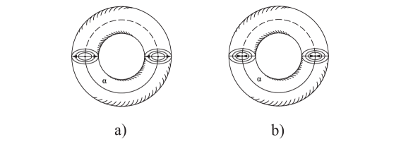
Figure 1: Index 2 (repeller) a), index 0 (attractor) b), $S^{1}-$type orbits.

It will be demonstrated below that both $S^{1}$and $T^{2}$ can serve as attractors, repellers or saddles. For $T^{2}$ the analogous situationis depicted in Fig.2.

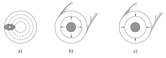
Figure 2: The ”orientable cylinder” whose boundaries are made out of two $T^{2\prime}s.$The repelling b) and the attracting c) tori $T^{2}.$

In the case of $T^{2}$ the following theorem by Wada is of importance

Theorem 5.9. Every indexed link which consists of all closed orbits of a NMS flow on S³ is obtained from (0,2) Hopf link by applying six operations. Convesely, every indexed link obtained from (0,2) Hopf link by applying these six operations is the set of all the closed orbits of some NMS flow on S${}^{3}\vskip 12.0pt plus 4.0pt minus 4.0pt\vskip 6.0pt plus 2.0pt minus 2.0pt$

These six Wada operations will be discussed in the next section. In the meantime we notice the following. Since by definition the NMS flow does not have fixed points on the underlying manifold $\mathit{M}$, use of the Poincare^′-Hopf index theorem  leads to $\chi(M)=0,$ where $\chi(M)$ is Euler characteristic of $\mathit{M}$.  It can be demonstrated that Euler characteristic for odd dimensional manifolds without boundary is zero  [$51$]. The proof for $\mathit{S}^{3}$ is especially simple and is provided below. Because of this, $\mathit{S}^{3}$ can sustain the NMS flow. The full implications of this fact were investigated by Morgan [$45$] (e.g. see Theorem 5.6.above). According to (now proven) geometrization conjecture every 3-manifold can be decomposed into no more than 8 fundamental pieces [$52,53$]. Morgan proved that any 3-manifold which does not contain a hyperbolic piece can sustain the NMS flows. This result is compatible with the Remark 5.5.

For $\mathit{S}^{3}$ the above results can be proven using elementary arguments. Specifically, let us notice that Euler characteristic of both $S^{1}$ and $T^{2}$ is zero.  In addition, it is well known that $S^{3}$ can be made out of two solid tori glued together. In fact, any 3-manifold admits Heegaard splitting  [$53$]. This means that it can be made by appropriately gluing  together two handlebodies whose surfaces are Riemannian surfaces of genus $g$. In our case $T^{2}$ is the Riemannian surface of genus one and the handlebody (solid torus) is $V=$ $D^{2}\times S^{1}$. It has $T^{2}$ as its surface. Consider now the Hopf link. It is made out of two interlocked circles. We can inflate these circles thus making two solid tori out of them. These tori (toric handlebodies) can be glued together. If the gluing h̄ is done correctly [$54,55$], we obtain $S^{3}$ as result. The following set-theoretic properties of Euler characteristic $\chi(M\cup N)=\chi(M)+\chi(N)-\chi(M\cap N)$  and $\chi(M\times N)=\chi(M)\cdot\chi(N)$ can be used now to calculate the Euler characteristic of $S^{3}.$ For the solid torus $V=$ $D^{2}\times S^{1}$ we obtain: $\chi(D^{2}\times S^{1})=\chi(D^{2})\cdot\chi(S^{1})=0$ since $\chi(S^{1})=0$ . Next  $S^{3}=(D_{1}^{2}\times S_{1}^{1})\cup_{\text{\={h}}}(D_{2}^{2}\times S_{2}^{1}),$ where h̄ is gluing homeomorphism h̄ $:$ $T_{1}^{2}\rightarrow T_{2}^{2}.$ Therefore $\chi(S^{3})=\chi(V_{1}\cup_{\text{\={h}}}V_{2})=\chi(V_{1})+\chi(V_{2})=0$ . Furthermore, the solid torus $V$ is the trivial case of the Seifert fibered space (see appendix E). Therefore $S^{3}$ is also Seifert fibered space [$56$]. According to Theorem 5.7. and Definition D.5 of Appendix D the NMS flows are made of finite number of periodic orbits which are either circles or tori. Thus, the NMS flows can take place on Seifert fibered manifolds or on graph manifolds.These are made of appropriately glued together Seifert fibered spaces  [$53$]. This conclusion is in accord with that obtained by Morgan [$45$] differently.

Let $(M)$ denote the class of all closed compact orientable 3-manifolds and $(H)$ denote the class of all closed compact orientable nonsingular isoenergic surfaces of Hamiltonian systems that can be integrated with help of the Bott integrals. Then, the following question arises: Is it always true that $(H)\subset(M)?$

There is a number of ways to construct 3-manifolds from elementary (prime) blocks  [$52,53$]. In particular, to answer the above question Fomenko [$24$] introduces 5 building blocks to be assembled. Four out of 5 blocks are associated with orientable manifolds. In this paper we shall discuss only these types of manifolds. They can be described as follows.

1.  The solid torus $D^{2}\times S^{1}$ whose boundary is $T^{2}.$

2.  The orientable ”cylinder”  $T^{2}\times D^{1}$, e.g. see Fig.2a). Its boundary of

is made out of two $T^{2}.$

3.  An ”orientable saddle” $N^{2}\times S^{1},$ e.g. see Fig.3a)

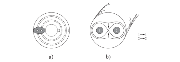
Figure 3: Orientable saddle a) and its bifurcation b)

Its boundary is made out of three $T^{2}.$

4. A ”non-orientable saddle”,  e.g. see Fig. 4a).

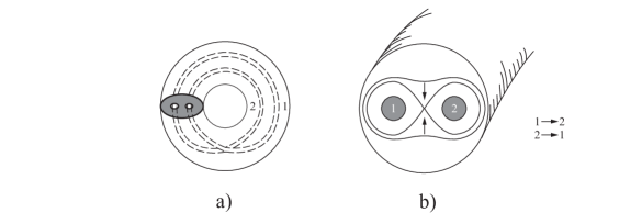
Figure 4: A  non-orientable saddle a) and its bifurcation b)

Its boundary is made out of two $T^{2}.$

Just by looking at these figures, it is clear that:

orientable cylinder= orientable saddle+solid torus

Theorem 5.10. Let $H=const$ be some isoenegy surface of some Hamiltonian system

integrable on H via Bott integral F.  Then H can be made by gluing

together a certain number of solid tori $D^{2}\times S^{1}$ and orientable saddles

$N^{2}\times S^{1},$ that is $H=\alpha(D^{2}\times S^{1})+\beta(N^{2}\times S^{1})$. 

The elementary manifolds are glued together via  diffeomorphisms of their boundary tori

It is symbolically denoted by the sign ”+”. Here $\alpha$ and $\beta$ are some  nonnegative integers

In 1988 Matveev and Fomenko [$57$] proved the following theorem (e.g. read Theorem 3 of this reference)

Theorem 5.11. A compact orientable 3-manifold with (possibly empty) torus-type

boundary belongs to the class (H) if and only if  its interior admits  a canonical

decomposition into pieces having geometries of the first seven types.

In particular, (H) contains no hyperbolic manifolds.

Remark 5.12. According to Thurston’s geometrization conjecture (now proven by G. Perelman) every 3-manifold admits a canonical decomposition into 8 basic building blocks (or geometries). Out of these, only one is hyperbolic, e.g. read Scott  [$52$].This result is fully consistent with earlier made Remark 5.5.

Corollary 5.13. Theorem 5.11.  provides an answer to the question ”Is it always true that $(H)\subset(M)?"\vskip 12.0pt plus 4.0pt minus 4.0pt$

In  view of Remark 5.5., Theorem 5.11. is of central importance for this paper. Because of this, we shall return to its content a number of times in what follows. In the meantime, in preparing results for the next section, using Fomenko’s [$24$] results, we need to reinterpret Wada’s results, that is  to describe how his results are related to bifurcations of the Arnol’d-Liouville tori. Bifurcations of these tori are caused by changes in the constant $c$ in the equation $F=c$ for the Bott integral. These are depicted in Fig.26 of Fomenko’s paper but, again, we do not need all of them. Those which we need can be easily described by analogy with 4 basic blocks described above. Our presentation is facilitated by results of Theorem 5.7. Using it, we conclude that in orientable case we have to deal only with $S^{1}$ and $T^{2}.$ Stability or instability of these structures cause us to consider along with them a nearby space foliated, say, by tori. Specifically,

1. A torus $T^{2}$ is contracted to the axial circle $S^{1}=\alpha$ and then, it may even vanish,

depending upon the value of $c$. Thus, we get $T^{2}\rightarrow S^{1}\rightarrow 0.$ Naturally, the process

can go in opposite direction as well, e.g. see Fig. 1 a) and b).

2. Two tori $T^{2}$ move toward each other (that is  they both flow into $T^{2})$ as depicted

in Fig.2 b) and c). Let, say, both  the outer boundary and the inner boundary be

unstable in the sense that there is a $T^{2}$ surface somewhere in between the inner

and the outer $T^{2\prime}s$ . Such a torus is as an attractor since both the inner and the

outer $T^{2\prime}s$ are being attracted  to it. In this case we may have the following

process: $2T^{2}\rightarrow T^{2}\rightarrow 0.$

Apparently, the process can go in reverse too. In such a case we are dealing with

repeller.

3. Imagine now a pair of pants. Consider a succession of crossections for such pants.

On one side, we will have $D^{2}($the waist). This configuration will continue till it will

hit the fork- the place from where the pants begin . The fork crossection

is made of figure 8. After passing that crossection we are entering

the pants.  This process is depicted  in Fig.3. We begin with the configuration

of Fig.2a), then the bifurcation depicted in Fig.3b) is taking place  resulting in

configuration depicted in fig.3 a).

Thus, initially we had $T^{2}$ and finally we obtained $2$ $T^{2}$.  That is now we have :

$\ \ T^{2}\rightarrow 2T^{2}.$

4. A non-orientable saddle  is obtained if for any crossection of $N^{2}\times S^{1}$ we can

swap the 1st $D_{1}^{2}$ $\subset T_{1}^{2}$ with $D_{2}^{2}$ $\subset T_{2}^{2}$ as depicted in Fig.4 a) and b). In such a case

we obtain: $T^{2}\rightarrow T^{2}.$ Such description of bifurcations is consistent with Theorem 5.7.

It can be demonstrated that the bifurcations 2 and 4 can be reduced to 1 and 3.

This fact will  be used in the next section.

Remark 5.14. Just described processes are expected to play major role in topological reinterpretation of scattering processes of high energy physics advocated in [$13$].  Very likely, the already developed formalism of topological quantum field theories (TQFT) and Frobenius algebras , e.g. as discussed in [$58$], could be used for this purpose. Alternatively, following ideas of Fomenko and Bolsinov book [$33$], and that by Manturov, e.g. read chapter 8 of [$59$], it might be possible to develop topological scattering theory using theory of virtual knots and links initiated by Kauffman [$60$].

6.     Dynamical bifurcations and topological transitions associated with them

6.1.  General remarks

In the previous section we mentioned works by Wada, Morgan and Fomenko-Zung related to dynamics of NMS flows. The focus of this paper however is not on these flows as such but rather on descriptions of mechanisms of generation of knotted/linked trajectories. Theorems 5.3. and 5.6. provide us with guidance regarding the types of knots/links which can be generated by the NMS flows. However, the above theorems do not explain how such knots/links  are actually generated. Wada’s results, summarized in Theorem 5.9., provide a formal description of the sequence of topological moves producing the iterated knots/links, beginning with the Hopf links. These moves are depicted in Fig.s 2-7 of the paper by Campos et al [$61$]. These are, still, just particular kinds of Kirby moves as explained in Appendix F. The description of these moves is totally disconnected from the description of dynamical bifurcations depicted in Fig.s 1-4 above. Fomenko [$24$] designed a graphical method helpful for understanding of the sequence of topological transitions. More details on this topic is given in the monograph by Fomenko and Bolsinov [$33$]. Remark 5.14. provides us with suggestions for the further development. Nevertheless, using the already obtained results, we are now in the position to explore still other ways for connecting Wada’s results with dynamical bifurcations. They are discussed in this section. In it, we develop our own approach to the description of topological transitions between dynamically generated knots/links.

6.2.   Generating cable and iterated torus knots

In view of Theorems 5.3 and 5.6. we need to provide more detailed description of the iterated torus knots/links first. For this purpose, following Menasco [$62$] we introduce  an oriented  knot $S^{1}\rightarrow$ $\mathit{K}\subset S^{3}.$ Let then $V_{K}$ be a solid torus neighborhood of $K$. Let $\partial V_{K}$ $=T_{K}^{2}\subset S^{3}.$ As in appendix E, we write

$$J\sim\nu\mathfrak{M}+\mu\mathfrak{L.}$$ (6.1)

This is the same equation as eq.(E.1a) describing a simple oriented closed curve $J$  going $\nu$ times around the meridian $\mathfrak{M}$ and $\mu$ times around the longitude $\mathfrak{L}$ of $T_{K}^{2}.$ $J$ belongs to the homotopy class $\pi_{1}(T_{K}^{2})$ if and only if either $\nu=\mu=0$ or $g.c.d(\mu,\nu)=1$ (Rolfsen [$55]$).

Definition 6.1. When $K$ is unknot, $K=K_{0}$, the curve $J$ is called ($\mu,\nu)$ a cable of $K$.  Thus, $K$($\mu,\nu)$ torus knot is a cable of the unknot. The cabling operation leading to the formation of $\mathit{K}$($\mu,\nu)$ torus knot from now on will be denoted as C($K_{0}$, ($\mu,\nu))$.

The above definition allows us to generate the iterated torus knot inductively. Beginning with some unknot $K_{0},$ we select a sequence of co-prime 2-tuples of integers $(P,Q)=\{(p_{1},q_{1})$,$(p_{2},q_{2}),\cdot\cdot\cdot,(p_{n},q_{n})\}$, where $p_{1}<q_{1}.$ This information allows us to construct the oriented iterated torus knot

$$\mathit{K(P,Q)}=\mathbf{C}(\mathbf{C}(\cdot\cdot\cdot\mathbf{C}(\mathbf{C(}K_{0},(p_{1},q_{1}))(p_{2},q_{2}))\cdot\cdot\cdot,(p_{n-1},q_{n-1})),(p_{n},q_{n})).$$ (6.2)

No restrictions on the relative magnitudes of  $p_{i}$ and $q_{i}$ are expected to be imposed for $n>1,$[$63$].

These general rules  can be illustrated using the trefoil knot $K(2,3)$ as an example. It is a cable of the unknot. Since the trefoil is the (simplest) torus knot  it can be placed on the surface of the solid torus. This torus has an unknot $K_{0}$ as the core. In Fig.5

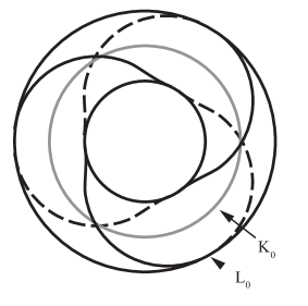
Figure 5: One of the ways to depict the trefoil knot

the core $K_{0}$ is depicted as a circle while the longitude of the solid torus around $K_{0}$ is labeled by $\mathit{L}_{0}.$ Without loss of generality both circles $K_{0}$ and $\mathit{L}_{0}$ are placed on the same plane $z=0$.   The projection of the knot $K(2,3)$ into the same z-plane intersects $L_{0}$ in $q=3$ points. Instead of  Fig.5, the same  configuration can be interpreted in terms of closed braids. For this purpose, following Murasugi [$64$],  the representation of torus knot $K(q,p)$ in terms of closed braids is depicted in Fig.6.

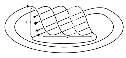
Figure 6: Braid-type presentation of the torus knot K(p,q)

Such a representation is not unique. It is so because $K(q,p)=K(p,q).$ Furthermore, $K(-q,p)$ is the mirror image of $K(q,p).$ If  $g.c.d(p,q)=1$, then $K(-q,-p)$ is the same torus knot but with the reverse orientation. Being armed with these results, we need to recall the presentation of the braid group B_n made out of $n$ strands. Its generators and relations are

$$\text{B}_{n}=\left(\sigma_{1},...,\sigma_{n-1}\mid\begin{array}[]{c}\sigma_{i}\sigma_{j}=\sigma_{j}\sigma_{i},\left|i-j\right|\geq 2\\ \sigma_{i}\sigma_{i+1}\sigma_{i}=\sigma_{i+1}\sigma_{i}\sigma_{i+1},i=1,2,...,n-2\end{array}\right).$$ (6.3)

The connection between the $K(q,p)$ and its braid analog depicted in Fig.6. can be also established analytically via

$$K(q,p)\Rightarrow(\sigma_{p-1}\sigma_{p-2}\cdot\cdot\cdot\sigma_{2}\sigma_{1})^{eq},$$ (6.4.)

where $e=\pm 1$ depending on knot orientation. Here the symbol $\Rightarrow$ means ”closure of the braid” -an operation converting braids into knots/links [$64$]. These general results adopted for the trefoil knot  are depicted in Fig.7.

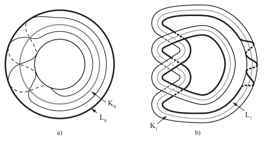
Figure 7: Braid-type presentation of the torus knot $K(2,3)$. In a) we use the same notations as in Fig.5 while in b) the core $K_{1}$ is in fact  our trefoil knot $K(2.3)$. Such braid-type presentation is the most convinient for developing the iteration process generating all iterated torus knots associated with K(2,3)

By design, the notations on this figure are meant to facilitate visualization of the iteration process. It is formalized in the following

Definition 6.2. Cabling operation. Let $K_{1}$ be an arbitrary oriented knot in $S^{3}$ and $N(K_{1})$ is its solid torus tubular neighborhood. Let furthermore $L_{K_{1}}$ be a longitude for $K_{1}$. It is a simple closed curve on $\partial N(K_{1})$ homologous to $K_{1}$ in $N(K_{1})$ and null- homologous in $S^{3}\smallsetminus K_{1}.$  Consider now a homeomorphism $h:N(K_{0})\rightarrow N(K_{1})$  which is also mapping $L_{0}$ into $L_{K_{1}}.$ By relabeling : $K_{0}\rightarrow K_{i}$ and $K_{1}\rightarrow K_{i+1}$ , the cabling operation C can be formally defined now as $h:N(K_{i})\rightarrow N(K_{i+1}),$ with $L_{i}$ being mapped into $L_{i+1}.\vskip 12.0pt plus 4.0pt minus 4.0pt$

Definition 6.3. A cable space C is a Seifert fibered manifold obtainable from the solid torus $S^{1}\times D^{2}$ by removing $N(K_{1})\subset S^{1}\times\mathring{D}^{2}$ from $S^{1}\times\mathring{D}^{2},\mathring{D}^{2}=D^{2}$ $\smallsetminus\partial D^{2}$. Thus, in accord with results of Appendix E, it is a Seifert fibered manifold having no exceptional fibers. Alternatively, following Jaco and Shalen [$65$], page 182, a cable space C can be defined as follows. Let $S$ be a Seifert fibered space over a disc $D^{2}$ with one exceptional fiber, then  the complement in $S$ of an open regular neighborhood of a regular fiber is a cable space C.

The validity of the above definition is based on the following

Theorem 6.4. (Hempel [$66$]) Let $V_{K}\subset S^{1}\times D^{2}$ be a tubular neighborhood of the torus knot $K$ (including the unknot) in $S^{3}$ and let $M$ be  a simply connected 3-manifold containing a solid torus $V$. Suppose that there is a homeomorphism $h$ of $S^{3}\smallsetminus$ $\mathring{V}_{K}$ onto $M\smallsetminus\mathring{V},$ then $M=S^{3}.$ 

Corollary 6.5. Due to the Heegaard decomposition, $S^{3}$ is always decomposable into two solid tori. Therefore, in view of the above homeomorphism, it is sufficient to replace $S^{3}$ by ( that is work with) solid torus $V=S^{1}\times D^{2}$  only. This provides a justification of the operations inside the solid torus depicted in Fig.12 (appendix F).

The information  we have accumulated allows us now to reobtain one of Zung and Fomenko’s results. Specifically, we have in mind the special toral windings leading to torus knots of the type $K(2,2l+1)$.  Now we are in the position  enabling us to explain the meaning of this result.

Since $K(q,p)=K(p,q)$, we obtain: $K(2,2l+1)=$ $K(2l+1,2)$ implying that we are dealing with torus knots made out of just 2 braids twisted $n=2l+1$ times followed by the closure operation making a knot out of them.  Adopted for such a case eq.(6.4) now reads: $K(n,2)\rightleftarrows(\sigma_{1})^{n}.$ Switching of just one crossing in the knot projection, e.g. see Fig.6,  makes $(\sigma_{1})^{n}$ to be replaced by $\sigma_{1}^{i}\sigma_{1}^{-1}\sigma_{1}^{j}$ so that $i+j-1=m$ . To find $m$ it is sufficient to notice that initially (that is before switching) we had $i+j+1=n.$ Thus, $i+j=n-1$ and, therefore, $n-2=m.$ In view of the property $K(q,p)\simeq K(-q,-p)$ it is sufficient to discuss only the case $m\geq 0$ leading to $n\geq 2.$ Since $n=2l+1$ we obtain $n=3$ when $l=1$ that is we are dealing with the trefoil $K(2,3)$. When $l=0$ we are dealing with the unknot and so on. The obtained result is consistent with the Kirby move depicted in Fig.17 (appendix F). Indeed,  we can always place the unknot into solid torus (Corollary 6.5). If we begin with the Hopf link, which is $\pm 1$ framed unknot, and fix our attention at one of the rings which is unknot, then another ring can be looked upon as framed with framing $\pm 1.$ Such type of framing converts another unknotted ring into the Hopf link again.

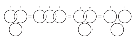
Figure 8: Physics behind this picture is charge conservation. It will explained later in the text

This situation is depicted in Fig.8. The extra ring can always be found in the spirit of Wada’s (1989) paper [$50$]. Say, we can  take the meridian of the solid torus into which the first unknotted ring of the Hopf ring was enclosed as an extra ring. In fact, this is the content of Theorem 2 by Menasco [$62$]. Thus, the Kirby moves depicted in Fig. 15 generate all special toral windings obtained in Fomenko and Zung paper.

With this result in our hands, we still have to uncover the topological mechanism by which the iterated torus knots are generated in order to recover the rest of Zung-Fomenko results and those obtained by Morgan (e.g. see Theorems 5.3.and 5.6.above). It is important to notice at this stage that torus knots are allowed in the NMS dynamics just because the Kirby-Fen-Rourke moves allow such knots to exist. These moves are not sufficient though for generation of the iterated torus knots/links. Following works by Milnor [$67$] and Eisenbud and Neumann [$68$] it is possible using  methods of algebraic geometry  to develop graphical calculus generating all iterated torus knots and links. Incidentally, in current physics literature one can find proposals for generating iterated torus knots/links via methods of algebraic geometry just cited. E.g. read Dennis et al  [$69$] or Machon and Alexander [$70$]. While methods of algebraic geometry are very effective for depicting knots/links, they are rather formal because they are detached from the topological content/mechanism of dynamical bifurcations generating various iterated torus knots. Thus, we are going to proceed with the topological treatment of dynamical bifurcations. For this purpose, following  Jaco (1980) [$71$], we begin with a couple of

Definition 6.6.  In accord with Theorem 6.4. a complement of a torus knot $K(p,q)$ in $S^{3}$ is the torus knot space.

Definition 6.7. An (n-fold) composing space is a compact 3-manifolds homeomorphic to $W(n)\times S^{1},$ where $W(n)$ the disk with n-holes

Remark 6.8. Evidently, previously defined cable space is just a special case of the composing space.

The complement of a link in $S^{3}$ made of a composition of $n$ torus-type knots (including the unknot(s)) is an n-fold composing space. An n-fold composing space is the Seifert fibered space in which there are no exceptional fibers (appendix E) and the base (the orbit space) is a disc with $n$ holes. Such a fibration of composing space is called standard. The following theorem summarizes what had been achieved thus far

Theorem 6.9. (Jaco and Shalen [$65$]), Lemma 6.3.4. A  Seifert-fibered 3-manifold $M(K)=S^{3}\smallsetminus\mathring{N}(K)$ with incompressible boundary $\partial M(K)=N(K)\smallsetminus\mathring{N}(K)$ is either a torus knot space, a cable space or a composing space.

Following Jaco [$71$], page 32, the incompressibility can be defined as follows. Set $M(K)=S^{3}\smallsetminus\mathring{N}(K),$ then $\partial M(K)=S^{1}\times S^{1}$ is incompressible in $M(K)$ iff $K$ is not an unknot.  A complement of  a cabled knot  in $S^{3}$ always contains a cabled space with incompressible boundary [$65$], page 182.

At this point we are having all the ingredients  needed for description of the bifurcation cascade creating iterated torus knots/links. The process can be described inductively. We begin with the seed- the cable space depicted in Fig.2a). The first bifurcation is depicted in Fig.s 3 a),b). It is producing the composing nonsingular Seifert fibered space whose orbit space is the disc $D^{2}$ with two holes. The homeomorphism depicted in Fig.12 allows us to twist two strands  as many times as needed. Thus, many (but surely not all!) iterated torus knots are going to have the same complements in $S^{3}.$ Clearly, the first in line of such type of knots is the trefoil knot $K(2,3)$ depicted in Fig.7a). It plays the centarl role in particle-knot correspondence [$13$]. Evidently, other knots of the type $K(p,q)$ are also permissible. Their complement is still going to be the two-hole composing space depicted in Fig.3.a). The three-hole composing space is generated now as follows. Begin with the composing space depicted in Fig.3.a). Use the bifurcation process depicted in Fig.3.b) and apply it to one of the two holes in Fig.3.a). As result, we obtain the three-hole composing space. Again, we can use the homeomorphisms to entangle the corresponding strands with each other.

The bifurcation sequence leading to creation of all types of iterated torus knots is made of steps just described.  It suffers from several deficiencies.  The first among them is a regrettable absence of the one-to one correspondence between the links and their complements, e.g. see Fig.12. The famous theorem by Gordon and Luecke [$72$] seemingly guarantees that the degeneracy is removed for the case of knots since it states that knots are being determined by their complements. This happens not always to be the case. Details are given in the next section. The second deficiency becomes evident already at the level of the trefoil knot which is the cable of the unknot, e.g. see Fig.7. In Fig.7a) we see that it is permissible to associate one strand of the two-holed composing space with the unknot while another-with the trefoil knot. At the same time, if we want to use braids, as depicted in Fig.7b), then we obtain 3 braids instead of two strands. Thus, we are coming to the following

Problem: Is there a description of the iterated torus knots in terms of braids as it is done, say, for the torus knots in Fig.6 ?

A connection between closed braids and knots/links is known for a long time. It is of little use though if we are interested in providing a constructive solution to the problem we had just formulated. Surprisingly, the solution of this problem is very difficult. It was given by Schubert [$73$]. Recently, Birman and Wrinkle [$63$] found an interesting interrelationship between the iterated torus knots, braids and contact geometry.This interrelationship happen to be of profound importance in studying of scattering processes in terms of particle-knot/link correspondence discussed in [$13$], Kholodenko (2015b). In view of this, we would like to discuss results of these authors in some detail in the next subsection.

6.3. Back to contact geometry/topology. Remarkable interrelationship

between the iterated torus  and transversely simple knots/links

6.3.1. Basics on Legendrian and transverse knots/links

In sections 5 and 6 results of contact geometry/topology obtained in sections 2-4 were used  but without development.  In this subsection we would like to correct this deficiency. For this purpose we need to introduce the notions of the Legendrian and transverse knots. As before, our readers are encouraged to consult books by Geiges [$14$] and Kholodenko [$6$] for details.

We begin with some comments on ”optical knots” which were defined in the Introduction section of part I. The term ”optical knots” was invented by Arnol’d [$74$] in connection with the following problem.

Solutions of the eikonal equation $\left(\partial S/\partial q\right)^{2}=1$ determine the optical Lagrangian submanifold $p=\partial S/\partial q$  belonging to the hypersurface $p^{2}=1.$ Every stable Lagrangian singularity is revealing itself  in the projection of the Lagrangian submanifold into the base ($q$-space), e.g. read Appendix 12 of Arnol’d book[$31$]. If these results are used in R${}^{3},$ then the base is just the whole or part of R${}^{2}.$ In such a case we can introduce the notion of a Legendrian knot. It originates from the equation $p=\partial S/\partial q$ written as $dS-pdq=0$ which we had already encountered in part I, section 4. This time to comply with literature on Legendrian knots  we are going to relabel the entries in the previous equation as follows

$$dz-ydx=0.$$ (6.5a)

The minus sign in front of $y$ is determined by the orientation of R${}^{3}.$ Change in orientation causes change in sign. The standard contact structure $\xi$ in the oriented 3-space $\mathbf{R}^{3}=(r,\phi,z),$ that is in cylindrical coordinates, is determined by the kernel ($\xi=\ker\alpha,$ that is by the condition $\alpha=0)$ of the 1-form $\alpha,$

$$\alpha=r^{2}d\phi+dz.$$ (6.5b)

(compare this result against the eq.(4.3))

Definition 6.11. A Legendrian knot $K_{L}$ in an oriented contact manifold $(M,\xi)$ is a circle $S^{1}$ embedded in $M$ in such a way that it is always tangent to $\xi.$ Let the indeterminate $\tau$ parametrize $S^{1}$  and choose $\mathbf{R}^{3}$ as $M$, then the embedding is defined by the map $f:$ $S^{1}\rightarrow\mathbf{R}^{3}$ specified either by $\tau\rightarrow(x(\tau),y(\tau),z(\tau))$ or by $f:\tau\rightarrow(r(\tau),\phi(\tau),z(\tau)).$ The coordinates $r(\tau),\phi(\tau),z(\tau)$ are real-valued periodic functions with period, say, $2\pi.$The tangency condition is being enforced by the equation

$$\frac{dz}{d\tau}=y(\tau)\frac{dx}{d\tau}.$$ (6.6)

Thus, whenever $\dfrac{dx}{d\tau}$ vanishes, $\dfrac{dz}{d\tau}$ must vanish as well.

Definition 6.12. In terms of $x,y,z$ coordinates it is possible to define either the front or the Lagrangian projection of the Legendrian knot. The front projection $\Pi$ is defined by

$$\Pi:\mathbf{R}^{3}\rightarrow\mathbf{R}^{2}:(x,y,z)\rightarrow(x,z)$$ (6.7)

The image $\Pi(K_{L})$ under the map $\Pi$ is called the front projection of $K_{L}.$ The condition, eq.(6.6), is causing the front projection not to contain the vertical tangencies to the $K_{L}$ projection.  Because of this, the front projection of the $K_{L}$ is made of  a collection of cusp-like pieces (with all cusps arranged in such a way that the cusp axis of symmetry is parallel to $x$-axis) joined between each other. The front projection is always having $2m$ cusps, $m\geq 1.$ It is important that these cusps exist only in the x-z plane, that is not in 3-space. The Lagrangian projection $\pi$ of the Legendrian knot $K_{L}$ is defined by

$$\pi:\mathbf{R}^{3}\rightarrow\mathbf{R}^{2}:(x,y,z)\rightarrow(x,y).$$ (6.8)

For the sake of space, we shall not discuss details related to the Lagrangian projection. They can be found in Geiges [$14$].

Remark 6.13. Arnol’d  optical knots are Legendrian knots. In geometrical optics such knots are also known as plane wavefronts. They obey the Hugens principle.

In addition to the Legendrian knots with their two types of projections  there are also transverse knots. They are immediately relevant to this paper. It can be shown that the topological knots/links can be converted  both to the Legendrian and to the transverse knots so that the transverse knots can be obtained from the Legendrian ones and vice versa [$14$], page 103. Since the Legendrian knots are also known as optical knots, this fact provides a justification for the titles of both parts I and II of this work.

Going back to the description of transverse knots, we begin with the

Definition 6.14. A transverse knot $K_{T}$ in contact manifold $(\mathbf{R}^{3},\xi)$ is a circle $S^{1}$ embedded in $\mathbf{R}^{3}$ in such a way that it is always transverse to $\xi.$ The transverse knots are always oriented. The front projection $\Pi(K_{T})$ must satisfy two conditions [$14,75$] graphically depicted in Fig.9

Figure 9: Forbidden configurations for the front projection of transverse knots

To formulate the meaning of the notion of transversality and of these conditions analytically, consider a mapping $\ f:$ $S^{1}\rightarrow\mathbf{R}^{3}:$ $\tau\rightarrow(x(\tau),y(\tau),z(\tau))$ with $x(\tau),y(\tau)$ and $z(\tau)$ being some periodic functions of $\tau$. The transversality condition now reads

$$\frac{dz}{d\tau}-y(\tau)\frac{dx}{d\tau}>0.$$ (6.9a)

This inequality defines the canonical orientation on $K_{T}.$ The front projection $\Pi(K_{T})$ is parametrized in terms of the pair $(x(\tau),z(\tau)).$ At the vertical tangency pointing down we should have $\frac{dx}{d\tau}=0$ and $\frac{dz}{d\tau}<0.$ This contradicts eq.(6.9a) thus establishing the condition a) in Fig.9.  The condition b) on the same figure is established by using eq.(6.9a) written in the form

$$y(\tau)<\frac{z^{\prime}}{x^{\prime}}.$$ (6.9b)

This inequality implies that y-coordinate is bounded by the slope $dz/dx$ in the x-z plane (the positive y-axis is pointing into the page). Etnyre [$75$] argues that this observation is sufficient for proving that the fragment depicted in Fig.9b) cannot belong to the fragment of the projection of $K_{T}.\vskip 12.0pt plus 4.0pt minus 4.0pt$

The importance of transverse knots for this paper is coming from their connection with closed braids studied in previous subsection. To describe this connection mathematically,  it is useful to introduce the cylindrical system of coordinates $(r,\phi,z)$ so that any closed braid can be looked upon as a map $f:S^{1}\rightarrow\mathbf{R}^{3}:\tau\rightarrow(r(\tau),\phi(\tau),z(\tau))$ for which $r(\tau)\neq 0$ and $\phi^{\prime}(\tau)>0$ $\forall\tau$ [$76$].

Definition 6.15. A link $L$ is $transverse$ if the restriction of $\alpha=r^{2}d\phi+dz$ to $L$  nowhere vanishes. Any conjugacy class in B_n defines a transverse isotopy class of transversal links/knots. Bennequin [$77]$ proved that any transverse knot/link is transversely isotopic to a closed braid.

Any knot $K$ $\subset\mathbf{R}^{3}$ belongs to its topological type $\mathcal{K}$, that is to the equivalence class under isotopy of the pair $(K$,$\mathbf{R}^{3}).$ In the case of transverse knots/links,  one can define the transverse knot type $\mathcal{T(K)}$. It is determined by the requirement $\frac{z^{\prime}(\tau)}{\phi^{\prime}(\tau)}+r^{2}(\tau)>0$ at every stage of the isotopy and at every point which belongs to the knot $K_{T}.$

In the standard knot theory knots are described with help of topological invariants, e.g. by the Alexander or Jones polynomials, etc.  Every transverse knot belongs to a given topological type $\mathcal{K}$. This means that the knot/link invariants such as Alexander or Jones polynomials can be applied. In addition, though, the transverse knots have their own invariant $\mathcal{T(K)}$ implying that all invariants for topological knots, both the Legendrian and transverse, should be now supplemented by the additional invariants. For the transverse knots in addition to $\mathcal{T(K)}$ one also has to use the  Bennequin (the self-linking) number $\beta(\mathcal{T(K))}$. To define this number, following Bennequin [$77$], we begin with a couple of definitions.

Definition 6.16.a) The $braid$ $index$ $n=n(K)$ of a closed braid $K$ is the number of strands in the braid

Definition 6.17.a) The algebraic length e(K) of the braid b

$$b=\sigma_{i_{1}}^{\varepsilon_{1}}\cdot\cdot\cdot\sigma_{i_{k}}^{\varepsilon_{k}}\in\text{B}_{n}$$ (6.10a)

prior to its closure resulting in knot  K  is defined  as

$$\mathit{e}(\mathit{K})=\varepsilon_{1}+\cdot\cdot\cdot+\varepsilon_{k}\in\mathbb{Z}\text{ .}$$ (6.10b)

Definition 6.18. The Bennequin number $\beta(\mathcal{T(K))}$ is defined as

$$\beta(\mathcal{T(K))=}e(K)-n(K).$$ (6.11)

Further analysis  [$63$] of  the results obtained by Bennequin ended in alternative definitions of the braid index and the algebraic length. Specifically, these authors came up with the following

Definition 6.16.b) The $braid$ $index$ $n=n(K)$ of a closed braid $K$ is the linking number of $K$ with the oriented z-axis

Definition 6.17.b) The algebraic crossing number e=e(K) of the closed braid is the sum of the signed crossings in the closed braid projection using the sign convention depicted in Fig.13.

A generic (front) projection of $K_{T}$ onto $r-\phi$ plane is called closed braid projection. Since the braid is oriented, the projection is also oriented in such a way that moving in the positive direction following the braid strand (along the z-axis direction) increases $\phi$ in the projection. To use these definitions effectively, we need to recall the definition of a writhe.

Definition 6.19. The writhe $w(K)$  of the knot diagram $D(K)$ (knot projection into plane R${}^{2})$ of an oriented knot is the sum of signs of crossings of $D(K)$ using the sign convention depicted in Fig.13.

From here it follows that if the z-axis is perpendicular to the plane R² we obtain $n(K)=0$ and

$$\beta(\mathcal{T(K))=}w(K).$$ (6.12)

This result is in accord with that listed in Etnyre [$75$] and Geiges [$14$], page 127, where it was obtained differently.

6.3.2.  Computation of writhe

For reasons which will become obvious upon reading and in view of eq.(6.12) we would like to evaluate $w(K)$ now. To do so,  choose the point $z=(z_{1},z_{2})=(x_{1}+iy_{1},x_{2}$ $+iy_{2})\in S^{3}$ and, at the same time, $z\in K_{T}.$ It is permissible to think about $z$ also as a point in R${}^{4}.$ Because of this, it is possible to introduce physically appropriate coordinate system in R⁴ as follows. Using eq.(3.5) we select the components of the Liouville vector field X , that is $\mathbf{X=(}x_{1}\mathbf{,}y_{1}\mathbf{,}x_{2}\mathbf{,}y_{2}\mathbf{),}$as the initial reference direction. Since $S^{3}$ is determined by the equation $x_{1}^{2}+y_{1}^{2}+x_{2}^{2}+y_{2}^{2}=1,$ or $\left|z_{1}\right|^{2}+\left|z_{2}\right|^{2}=1,$ we obtain $z_{1}dz_{1}+z_{2}dz_{2}=0.$ This is an equation for a hyperplane $\xi$ ($\xi=\ker\alpha,$ where $\alpha$ is defined by eq.(4.3)).

Recall that, say, in R³ the plane $\mathcal{P}$ is defined as follows. Let $X_{0}=(x_{0},y_{0},z_{0})$ $\in\mathcal{P}$. Let the normal N to $\mathcal{P}$ is given by N$=(a,b,c)$ where both $X_{0}$ and N vectors are determined with respect to the common origin. Then, $\forall$ $X=(x,y,z)\in\mathcal{P}$ the equation for the plane is  N$\cdot(\mathbf{X}-\mathbf{X}_{0})\equiv$N$\cdot d\mathbf{X}=0$. To relate the complex and real cases, we rewrite $z_{1}dz_{1}+z_{2}dz_{2}=0$ as $z\cdot dz=0$. This result is not changed if we replace $dz$ by $idz$. In such a case, the vector $\mathbf{X}$ is being replaced by $\mathbf{\tilde{X}}=$ $\mathbf{(-}y_{1}\mathbf{,}x_{1}\mathbf{,-}y_{2}\mathbf{,}x_{2}\mathbf{).}$ Eq.s (3.5) and (3.11)  help us  to recognize in $\mathbf{\tilde{X}}$ the Reeb vector field. Evidently, the equation $z_{1}dz_{1}+z_{2}dz_{2}=0$ defining the contact structure $\xi$ ($\xi=\ker\alpha)$ is compatible now with the condition of orthogonality $\mathbf{X}\cdot\mathbf{\tilde{X}}=0$ in R⁴.

In section 4 we established that the Reeb vector field is proportional to a) the Hamiltonian vector field and to b) the Beltrami vector field. Therefore, the knot/link transversality requires us to find a plane $\mathcal{\tilde{P}}$ such that the Beltrami-Reeb vector field X̃ is pointed in the direction orthogonal/transversal to the contact plane $\mathcal{\tilde{P}}$.  To find this plane unambiguously, we have to find a set of mutually orthogonal vectors X, X̃, X̆ and $\mathbf{\check{X}}$ which span R⁴. By keeping in mind that R⁴ is a symplectic manifold into which the contact manifold $S^{3}$ is embedded, we then should adopt these vectors to $S^{3}$. Taking into account that the Liouville field X is orthogonal to the surface $\left|z_{1}\right|^{2}+\left|z_{2}\right|^{2}=1$ we can exclude it from consideration. Then, the velocity $\mathbf{\dot{x}}(\tau)$ of any curve $\mathbf{x}(\tau)=(x_{1}(\tau),y_{1}(\tau),x_{2}(\tau),y_{2}(\tau))$ in $S^{3}$ admits the following decomposition [$35$]

$$\mathbf{\dot{x}}(\tau)=a(\tau)\mathbf{\breve{X}+}b(\tau)\mathbf{\check{X}+}c(\tau)\mathbf{\tilde{X}.}$$ (6.13)

To understand the true meaning of this result, we shall borrow some results from our book [$6$]. In it we emphasized that contact geometry and topology is known under different names in different disciplines. In particular, we explained that the basic objects of study in sub-Riemannian and contact geometries coincide. This gives us  a permission to re interpret the obtained results in the language of sub-Riemannian geometry.

By means of contactomorphism: $(x,y,z)\rightarrow(x,y,\frac{1}{2}xy-z),$ the standard 1-form of contact geometry $\alpha=dz+xdy$ after subsequent replacement of $z$ by $t/4$  acquires the following look

$$\alpha=-\frac{1}{4}dt+\frac{1}{2}(ydx-xdy).$$ (6.14a)

This form vanishes on two horizontal vector fields

$$\mathbf{X}_{1}=\partial_{x}+2y\partial_{t}\text{ and }\mathbf{X}_{2}=\partial_{x}-2y\partial_{t}.$$ (6.14b)

Mathematically, the condition of horizontality is expressed as

$$\alpha(\mathbf{X}_{i})=0,i=1,2.$$ (6.14c)

The Reeb vector field $\mathbf{R}$ is obtained in this formalism as a commutator:

$$[\mathbf{X}_{1},\mathbf{X}_{2}]=-4\partial_{t}\equiv\mathbf{R}.$$ (6.14d)

Clearly, this commutator is sufficient for determination of $\mathbf{R}$. It was demonstrated in [$6,35$] that the above commutator is equivalent to the familiar quantization  postulate $[q,p]=i\hbar I.$ That is, the commutator, eq.,(6.14d) defines the Lie algebra for the Heisenberg group. This group has 3 real parameters so that the Euclidean space R³ can be mapped into the space of Heisenberg group. Because of the commutator, eq.(6.14d), it follows that the motion in the 3rd (vertical) dimension is determined by the motion in the remaining two (horizontal) dimensions so that R${}^{3}=\mathbf{R}^{2}\times\mathbf{R}^{1}$.

Remark 6.20. This is the simplest form of the Holographic principle used in high energy physics. It also lies at the foundation of the sub-Riemannian geometry.

Specifically, let us suppose that we are having a curve $\mathbf{x}(s)=(x(s),y(s),t(s))$ in R${}^{3}.$ Its velocity vector $\mathbf{\dot{x}}(s)$ can be decomposed as

$$\mathbf{\dot{x}}(s) = \dot{x}\partial_{x}+\dot{y}\partial_{y}+\dot{t}\partial_{t}=\dot{x}(\partial_{x}+2y\partial_{t})-2\dot{x}y\partial_{t}$$ (5)

$$+\dot{y}(\partial_{x}-2y\partial_{t})+2\dot{x}y\partial_{t}+\dot{t}\partial_{t}$$

$$= \dot{x}\mathbf{X}_{1}+\dot{y}\mathbf{X}_{2}-\frac{1}{4}(\dot{t}+2x\dot{y}-2y\dot{x})\mathbf{R}\TCItag{6.15}$$

so that the curve $\mathbf{x}(s)$ is horizontal if $\ \dot{t}+2x\dot{y}-2y\dot{x}=0.$ This condition is equivalent to the condition $\xi=\ker\alpha$ introduced before, e.g. see eq.(6.6), in connection with the Legendrian knots/links. Thus, the decomposition given by eq.(6.15) for the contact manifold R³ should be replaced now by the decomposition given by eq.(6.13) for $S^{3}.$ In spite of the apparent differences in appearance between these two results, they can be brought into correspondence with each other. For this purpose, following Geiges [$14$], pages 76 and 95,  we need to construct the neighborhood of a transverse knot/link. Since any knot $K$ is just an embedding of $S^{1}$ into $S^{3}($or R${}^{3}),$ locally we can imagine $S^{1}$ piercing a plane $\mathcal{P}$ perpendicularly. Such a plane can be spanned, say, by the vectors $\mathbf{X}_{1}$ and $\mathbf{X}_{2}$ we just had described. Clearly, this makes our knot/link transverse and the neighborhood of $K_{T}$ is described by the two conditions

$$a)\text{ }\gamma_{T}:=(\theta,x=0,y=0)\text{ and }\theta\in S^{1};\text{ \ b) }d\theta+xdy-ydx=0.$$ (6.16)

The contact structure $\xi=\ker\alpha$ is determined by eq.(6.14a)) in which the ”time $t$” coordinate is compactified to a circle $S^{1}$. Once this is done we immediately recognize that:

a) The contact structure in the present case is exactly the same as can be obtained from the one-form $\tilde{\alpha}=\frac{r_{1}^{2}}{r_{2}^{2}}d\phi_{1}+d\phi_{2}$ we have introduced earlier.

b) The locality of the result, eq.(6.16), makes it not sensitive to the specific nature of knot/link. In particular, it remains valid for the Hopf link too.

These observations were proven previously by Bennequin [$77$] who derived them differently and formulated them in the form of the

Theorem 6.21. (Bennequin [$77$], Theorem 10) Every link transversal to standard contact structure on $S^{3}($given by our eq.(4.3)), transversally isotopic to a link L whose tangent $TL$ at any point which belongs to $L$ is arbitrarily close to the tangent to the fibre of the Hopf fibration.

To take full advantage of this result we have to make several additional steps. For this purpose we have to use the quaternions. Recall, that the quaternion $q$ can be represented as $q=z_{1}+j\bar{z}_{2}=(z_{1},\bar{z}_{2}),$ where $j$ is another complex number, $j^{2}=-1,$ such that $ij=-ji$ . Formally, there is also the third complex number $k$, $k^{2}=-1.$ In view of the definition of $q$ and the commutation  relation $ij=-ji$ its use can be by-passed. In view of just defined rules, $jq=jz_{1}+j^{2}\bar{z}_{2}=-\bar{z}_{2}+jz_{1}=(-\bar{z}_{2},\bar{z}_{1})$.  The obtained result we use to encode yet another vector $\mathbf{\breve{X}}=$ $\mathbf{(-}x_{2}\mathbf{,}y_{2}\mathbf{,}x_{1}\mathbf{,-}y_{1}\mathbf{)}$ in R${}^{4}.$  This vector was introduced by Bennequin without derivation. With the vectors X, X̃ and X̆ just defined, we notice that they are mutually orthogonal in R⁴ by design. Instead of 3 tangent vectors X₁,X₂ and R which span R³ now we have 4 vectors which span R⁴. These are X, X̃, X̆ and $\mathbf{\check{X}=(-}y_{2},-x_{2},y_{1},x_{1}).$ The last vector is written in accord with that used by Hurtado and Rosales [$78$]. In this paper the remaining three vectors also coincide with ours. When adopted to $S^{3},$ three vectors are tangent to $S^{3}$ and one, that is X, is normal to $S^{3}.$ Thus, it is sufficient to consider only the vectors which span the contact manifold $S^{3}.$ In such a case the analog of the commutator, eq.(6.14d), is given by

$$[\mathbf{\breve{X}},\mathbf{\check{X}]=-}2\mathbf{\tilde{X}.}$$ (6.17)

In accord with eq.(6.14d)), $\mathbf{\tilde{X}}$ is the Reeb vector field. The associated contact 1-form was defined in part I, eq.(4.14), as

$$\alpha=-y_{1}dx_{1}+x_{1}dy_{1}-y_{2}dx_{2}+x_{2}dy_{2}.$$ (6.18)

In the present case the horizontality conditions   are: $\alpha($X̌$)=\alpha(\mathbf{\breve{X}})=0.$ Obtained information is sufficient for explanation of the expansion given in eq.(6.13) (to be compared with eq.(6.15)) and, hence, for utilization of Theorem 6.21. Results of this theorem are in accord with the results obtained by Wada (Theorem 5.9.) stating the the standard Hopf link serves as the seed generating  all oriented iterated torus knots. Being armed with these results, now we are in the position to evaluate (to estimate) the writhe in eq.(6.12). Geiges [$14$] page 128, proved the following

Theorem 6.22. Every integer can be realized as the self-linking number (that is writhe) of some transverse link

This theorem is providing only a guidance to what to expect. More useful is the concept of transversal simplicity

Definition 6.23. A transverse knot is transversely simple if it is characterized (up to transversal isotopy) by its topological knot type $\mathcal{K}$ and by $\beta(\mathcal{T(K))}$.

By definition, in the case of a link $\beta(\mathcal{T(K))}$ is the sum of $\beta(\mathcal{T(K))}$ for each component of the link. Thus, the m-component unlink is transversely simple since the unknot is transversely simple. To go beyond these obvious results requires introduction of the concept of exchange reducibility. Leaving details aside (e.g. read Birman and Wrinkle [$63$], it is still helpful to notice the following.

Closed n-braid isotopy classes are in one-to-one correspondence with the conjugacy classes of the braid group B_n. This result survives under the transverse isotopy. Such isotopy preserves both $n(K)$ and $e(K).$ In addition to the isotopy moves, there are positive/negative ($\pm)$ destabilization moves. The destabilization move reduces the braid index from $n$ to $n-1$ by removing a trivial loop. If such a loop contains a positive crossing, the move is called positive (+). The move reduces $e(K)$ by one and thus preserves $\beta(\mathcal{T(K))}$. The negative destabilization (-) increases $\beta(\mathcal{T(K))}$ by 2.  Finally, there is an exchange move. It is similar to the 2nd Reidemeister move. It changes the conjugacy class and, therefore, it cannot be replaced by the braid isotopy. Nevertheless, an exchange move preserves  both $n$ and $e$ and, therefore, also $\beta(\mathcal{T(K))}$. Clearly, these moves allow us to untangle the braid of $n$ strands and to obtain the unlink whose projection is made of $m$ unknots.

Definition 6.24. A knot of type $\mathcal{K}$ is exchange reducible if a closed n-braid representing this knot  can be changed by the finite sequence of braid isotopies, exchange moves and $\pm$ destabilizations to the minimal m-component unlink $m=n_{\min}(\mathcal{K}).$ In such a case max$\beta(\mathcal{T(K))}$ is determined by $n_{\min}(\mathcal{K}).$ For the iterated torus knots the exact value of max$\beta(\mathcal{T(K))}$ , that is of $n_{\min}(\mathcal{K}),$is known. In view of eq.(6.12) we finally obtain

$$max\beta(\mathcal{T(K))=}n_{\min}(\mathcal{K})=w(K).$$ (6.19)

6.3.3. Implications for the interated torus knots

Based on just obtained result, it  is possible to prove the following

Theorem 6.25. If $\mathit{K}\in\mathcal{T(K)}$ such that $K$ is exchange reducible, then  it is transversely simple.

Proof of this theorem allows to prove the theorem of central importance

Theorem 6.26. The oriented iterated torus knots are exchange reducible. Thus they are transversely simple.

Question: Are all knot types $\mathcal{K}$, when converted to transverse knot types $\mathcal{T}$($\mathcal{K}$) transversely simple?

Answer: No!

It happens, Etnyre [$75$], that transversely simple knots comprise a relatively small subset of knots/links. It is being made of:

a) the unknot;

b) the torus and iterated torus knots;

c) the figure eight knot.

From the results we obtained thus far we know that the figure eight knot cannot be

dynamically generated (Theorem 5.11). Thus, the transversal simplicity is not equivalent to

the previously obtained correspondence for flows: Beltrami$\rightarrow$Reeb$\rightarrow$Hamiltonian.

Question: Is this fact preventing generation of hyperbolic optical knots of which the figure eight knot is the simplest representative ?

Answer: No! The explanation is provided in the next section.

Remark 6.27. Theorem 6.26 allows to develop particle- knot/link correspondence constructively when superimposed with the Dehn surgery $-$ crosssing change correspondence discussed in Kholodenko (2015b).

7.     From Lorenz equations to cosmetic knots/links

In the previous section we described in detail  the cascade of bifurcations  generating  all possible torus and iterated torus knots and links dynamically. These results are sufficient for their use in high energy physics applications  described in Kholodenko (2015b). In this section we would like to discuss, also in detail, how other types of knots/links can be generated  and why these other types should not be considered in potential high energy physics applications. We begin with discussion of the classical works by Birman, Williams and Ghys.

7.1.  Birman-Williams treatment of the Lorenz equations           

Using methods of topological and symbolic dynamics Birman and Williams (BWa)) [$16$] explained the fact that flows generated by eq.s(4.5b) are special cases of those which follow from the description of periodic orbits of Lorenz equations. These  equations were discovered by Lorenz  in 1963 who obtained them as finite-dimensional reduction of the Navier-Stokes equation. Lorenz equations are  made of a coupled system of three ordinary differential equations.

$$\dot{x} = -10x+10y,$$

$$\dot{y} = rx-y-xz,\TCItag{7.1}$$ (6)

$$\dot{z} = -8/3z+xy.$$

Here $r$ is real parameter, the Rayleigh number. It is typically taken to be about 24. The equations are not of the Hamiltonian-type since they contain dissipative term. Accordingly, the results of previous sections cannot be immediately applied. Nevertheless, the results of BWa) paper are worth discussing  because of the following key properties of these equations. They can be summarized as follows.

1.  There are infinitely many non equivalent Lorenz knots/links generated by

closed/periodic orbits of eq.s(7.1).

2.  Every Lorenz knot is fibered.

3.  Every algebraic knot is a Lorenz knot.

From the previous section it follows that all iterated torus knots/links are of

Lorenz-type since they are algebraic.

4.  There are Lorenz knots which are not iterated torus knots; there are

iterated torus knots which are Lorenz but not algebraic.

5.  Every Lorenz link is a closed positive braid, however there are closed

positive braids which are not Lorenz.

6.  Every non-triviual Lorenz link which has 2 or more components is non splittable.

7.  Non-trivial Lorenz links  are non-amphicheiral. The link $L$ is amphicherial

if there is an orientation-reversing homeomorphism H: $(S^{3},L)\rightarrow(S^{3},L)$ reversing

orientation of $L$.  Because the Lorenz links are non-amphicheiral,

they are oriented links. From the Definition 6.14 we know that all transverse

knots/liks are oriented. Thus, all Lorenz knots/links are subsets of transverse

knots/links

8.  Non-trivial Lorenz links have positive signature. This technical concept is explained

in Murasugi [$64$]. In Kholodenko (2015b) the the signature is given

physical interpretation.

7.2.   Birman-Williams (1983b)) paper $[17$]. The universal template and the

Moffatt conjecture

BWa) study of periodic orbits was greatly facilitated by the template construction invented in their work. See also Ghrist et al [$37$] ,

Gilmore and Lefranc [$38$] and Ghrist [$79$] for many detailed examples.

Definition 7.1. A template $\mathcal{T}$  is a compact branched two-manifold with boundary built from finite number of branch line charts.

The key justification for introduction of templates can be explained as follows. Upon embedding of $\mathcal{T}$  into $S^{3}$ the periodic orbits of (e.g. Lorenz) semiflow tend

to form knots/links. In BWa) we find a

Conjecture 7.2. There does not exist an embedded $\mathcal{T}$ supporting all (tame) knots/links as periodic orbits, that is the are no universal template.

Definition 7.3. An universal template is an embedded template $\mathcal{T}\subset S^{3}$ among whose close orbits can be found knots of every type.

In 1995 guided by Birman and Williams (BWb) [$17$] Ghrist designed an universal template thus disproving the Birman-Williams conjecture. The full proof was subsequently published in [$18$]. Etnyre and Ghrist [$2$] took the full advantage of this fact and came up with the existence-type proof of the Moffatt conjecture  formulated by Moffatt in 1985 [$3$] . Recall, that this conjecture is claiming that in steady Euler flows there could be knots of any types. From results presented thus far in parts I and II it should be clear that the same conjecture is applicable to optical knots. More recently, Enciso and Peralta-Salas [$23$] produced also the existence-type proof of the Moffatt conjecture for Eulerian steady flows. These existence-type results are incompatible with the Beltrami$\rightarrow$Reeb$\rightarrow$Hamiltonian flows correspondence and, accordingly, with the Theorem 5.3. and its numerous corollaries.

Question: Is there way out of the existing controversy?

Answer: Yes, there is. It is based on the discussion of specific experimentally realizable set ups for generating knots/links of different types.

The first example of such a set up was discussed in great detail already in the B-Wb) paper in which the following experiment was considered. Suppose we are given a knotted piece

of wire with steady current flowing through the wire. The task lies in describing the magnetic field in the complement of such knot.

7.3.  Physics and mathematics of experimental design

In BWb) paper the authors discussed knotted magnetic field configurations surrounding a piece of wire coiled in the shape of figure 8 knot. From knot theory it is known that the Seifert surface of figure 8 knot  is punctured torus. Remarkably, but the punctured torus is also Seifert surface for the trefoil knot. The trefoil knot is a torus knot  and, therefore, it can be generated mechanically as was discussed in previous sections. Thus the discussion of similarities and differences between these knots will help us to resolve the controversy described in the previous subsection. In fact, discussions related to the trefoil knot will also be helpful for alternative description of the Lorenz knots which happens to be very illuminating.

The experimental set up not necessarily should involve compliance with eq.s(2.1a,b). For instance, if we use wires which are ordinary conductors, then we immediately loose both eq.s(2.1a,b) and all machinery we discussed thus far is going to be lost. This fact is also consistent with Theorem 5.3. The correspondence between physics of incompressible ideal Euler fluids and physics of superconductors was noticed in the paper by Fröhlich [$80$] but, apparently, was left non appreciated till publication of our book  [$6$] . The first 3 chapters of the book provide needed background for recognition of the fact that the correct set up realizing the requirements given by eq.s (2.1a,b) is possible only if we are using superconducting wires. In part I and at the beginning of part II we discussed the Hopf links  made of two linked unknotted rings. If one of the rings is made out of supercoducting wire, then the magnetic field in this wire will be collinear with the direction of the superconducting current. The superconducting current, in turn, will create yet another magnetic field and, since the magnetic field does not have sources or sinks, we end up with the Hopf link. In the present case, we have instead of superconducting circle (that is of an unknot) a superconducting coil $K$ in the form of the trefoil or figure 8 knot. The magnetic field collinear with the current in the circuit obeys eq.s (2.1a,b), as required,  while the surrounding magnetic field will live in $S^{3}\smallsetminus K$ space and should not be consistent with eq.s (2.1a,b). Thus, we are left with the problem of describing all knotted/linked structures in the space $S^{3}\smallsetminus K$ . We begin this description in the next subsection.

7.4.  Some facts about fibered knots

Both the trefoil and figure eight knots are the simplest examples of fibered knots. We discussed both of them in detail in[81] in the context of dynamics of 2+1 gravity. This circumstance greatly simplifies our tasks now. From previous sections we know that the trefoil knot can be generated  with help of  methods of Hamiltonian and contact dynamics while the figure eight knot cannot. Nevertheless, both of them are having the same Seifert surface $S-$the punctured/holed torus. An orientation-preserving surface homeomorphisms $h:$ $S\rightarrow S$ of the holed torus should respect the presence of a hole. This is so because the circumference of this hole is our knot (trefoil or figure eight).

The mapping torus fiber bundle $T_{h}$ can be constructed as follows. Begin  with the products $S\times 0$ (the initial state) and $S_{h}\times 1$ (the final state) so that for each point $x\in S$ we have $(x,0)$ and $(h(x),1)$ respectively.  After this, the interval $I=(0,1)$ can be made closed (to form a circle $S^{1}).$This is achieved by identifying $0$ with $1$ causing the identification $h:$ $(x,0)=(h(x),1).$ The fiber bundle $T_{h}$  is constructed now as a quotient

$$T_{h}=\frac{S\times I}{h}.$$ (7.2)

It is a 3-manifold which fibers over the circle $S^{1}$. Such constructed 3-manifold in $S^{3}$ is complimentary to the (fibered) knot, in our case the figure eight or trefoil knot.

It happens that every closed oriented 3-manifold $M$ admits an open book decomposition. This means the following. An oriented link $L\subset M,$ called binding can be associated with locally trivial bundle p: $M\smallsetminus L\rightarrow S^{1}$ whose fibers are open (Seifert) surfaces $F_{S},$called pages. Technically speaking, $L$ is also required to have  a tubular neighborhood $L\times D^{2}$ so that the restricted map p: $L\times(D^{2}\smallsetminus\{0\})\rightarrow S^{1}$ is of the form $(x,y)\rightarrow y/\left|y\right|.$ The closure of each page $F_{S}$ is then  a connected compact orientable surface with boundary $L$. Any oriented link $L\subset M$ that serves as a binding of an open book decomposition of $M$ is called fibered link/knot.

There is a deep relationship between the Alexander polynomial $\Delta_{K}(t)$ for the fibered knot $K$ and the associated with it 3-manifold $\mathit{M}$. If $V$ be the Seifert matrix of linking coefficients for $K$, then $\Delta_{K}(t)=\det(V^{T}-tV).$ If the knot $K$ is fibered, the polynomial $\Delta_{K}(t)$ possess additional symmetries. Specifically, in such a case we obtain

$$\Delta_{K}(t)=\mathop{\displaystyle\sum}\limits_{i=0}^{2g}a_{i}t^{i}$$ (7.3)

and it is known that $\Delta_{K}(0)=a_{0}=a_{2g}=\pm 1.$ Here $g$ is the genus of the associated Seifert surface. Thus, fibered knots can be recognized by analyzing their Alexander polynomial. It is monic for fibered knots. Furthermore, using just described properties of $\Delta_{K}(t),$ we obtain as well $\Delta_{K}(0)=\det(V^{T})=\det(V)=\pm 1.$ Because of this, we obtain:

$$\Delta_{K}(t)=\det(V^{-1}V^{T}-tE)\equiv\det(M-tE).$$ (7.4)

Here $E$ is the unit matrix while $M=V^{-1}V^{T}$ is the monodromy matrix responsible for the surface homeomorphisms $h:$ $S\rightarrow S.$ In the case of figure 8 knot BWb) use

$$M_{a}=\left(\begin{array}[]{cc}2&1\\ 1&1\end{array}\right)$$ (7.5a)

while below, in eq.(7.20), it is shown that there is yet another matrix

$$M_{b}=\left(\begin{array}[]{cc}2&-1\\ -1&1\end{array}\right)$$ (7.5b)

participating in these homeomorphisms. Both matrices produce $\Delta_{K_{8}}(t)=t^{2}-3t+1.$ The matrix $M$  for the trefoil knot T is different. It is either

$$M_{a}=\left(\begin{array}[]{cc}1&1\\ -1&0\end{array}\right)\text{ or }M_{b}=\left(\begin{array}[]{cc}1&-1\\ 1&0\end{array}\right)$$ (7.6a,b)

producing $\Delta_{K_{\text{T}}}(t)=t^{2}-t+1.$ The 3-manifolds $T_{h}$ associated  with the figure 8 and trefoil knots are different because of the difference in the respective monodromy matrices.  The 3-manifold for the figure 8 knot is hyperbolic while for the trefoil it is Seifert-fibered.

Since locally, the complement of the figure 8 knot is behaving as the space of constant negative curvature the figure 8 knot is hyperbiolic knot. In hyperbolic space the nearby dynamical trajectories diverge. Nevertheless, Ghrist [18]  using BWb) was able to prove the following

Theorem 7.4. (Ghrist) Any fibration of the complement of the figure -eight knot in $S^{3}$ over $S^{1}$ induces a flow on $S^{3}$ containing every tame knot and link as closed orbits.

The proof of this result involves explicit design of the universal template which was used subsequently by Etnyre and Ghrist [$2$] in proving the Moffatt conjecture. These knots and links are not generated as Hamiltonian flows though. Nevertheless, in view of the above theorem the complement in $S^{3}$ of  the superconducting current carrying wire coiled in the shape of figure 8 knot  is expected to contain magnetic lines  of any (tame) knot and link.

In developing their proof Etnyre and Ghrist [2] (2000a) needed to combine the results of [$18$] with those coming from contact geometry. The specific contactomorphisms described in  section 4 are sufficient only for generation of torus and the iterated torus knots. The experimental set up discussed in previous subsection provides an opportunity to enlarge the collection of knots. In the following subsections we provide some details  of how this can be achieved.

7.5.  Lorenz knot/links  living in the complement of the trefoil knot

We begin by noticing that the trefoil knot can be generated dynamically, on one hand, and can be created by a superconducting piece of wire coiled in the form of the trefoil knot, on another hand. In both cases  the complements of the trefoil in $S^{3}$ are Seifert-fibered 3-manifolds [$71$]. The well known theorem by Gordon and Luecke [$72$] is telling us that knots are determined by their complements. This restriction is not extendable to links though as discussed in Appendix F. Following Ghys [$27$], and Ghys and Leys [$82$], we shall focus now at the complement of the trefoil knot.

We begin by discussing  in some detail the fiber bundle construction for the trefoil knot whose Seifert surface $S$ is the punctured torus. The homeomorphisms of $S$ are generated by the sequence of Dehn twists. The torus  can be visualized in a variety of ways. For example, as some cell of the square-type lattice whose opposite sides are being identified. The punctured torus would require us in addition to get rid of the vertices and of neighborhoods of these vertices.  The sequence of Dehn twists acting on the punctured torus relates different square-type lattices to each other. Should the puncture be absent, the elementary cells of these different lattices upon identification of opposite sides would be converted to different tori. Closed geodesics on these tori would correspond to different torus knots. Presence of the puncture complicates matters considerably, e.g. read [$83$].

Let $G=\pi_{1}(S)$ be the fundamental group of a surface and $P\subseteq G$ be the set of peripheral elements, that is those elements of $G$  which correspond to loops freely homotopic to the boundary components. For the punctured torus, $G$ is just a free group of two generators $a$ and $b.$ That is $G=<a,b\mid>.$ The subset $P$ is determined by the commutator $aba^{-1}b^{-1}\equiv[a,b].$ If generators $a$ and $b$ are represented by the matrices, then it can be shown that the presence of the puncture is reflected in the fact that $tr[a,b]=-2.$ The question arises: is it possible  to find $a$ and $b$ explicitly based on this information?  Notice, because of the puncture Euler characteristic $\chi$ of the torus becomes -1. This means that the covering space is H² that is it is the Poincar$e^{\prime}$ upper half plane or, which is equivalent, the Poincare disc $\mathcal{D}$. The group of isometries of $\mathcal{D}$ is $PSL(2,\mathbf{R}).$ Its closest relative is $SL(2,\mathbf{R})$. It is possible to do all calculations using $SL(2,\mathbf{R})$ and only in the end to use the projective representation. For matrices of $SL(2,\mathbf{R})$ the following identities are known

$$2+tr[a,b] = \left(tra\right)^{2}+\left(trb\right)^{2}+\left(trab\right)^{2}-\left[tra\right]\text{ }\cdot\left[trb\right]\cdot\text{ }\left[trc\right],$$

$$\left[tra\right]\text{ }\cdot\left[trb\right] = trab+trab^{-1}.\TCItag{7.7}$$ (15)

Since we know already that $tr[a,b]=-2$ the above identities can be rewritten as

$$x^{2}+y^{2}+z^{2}=xyz;\text{ }xy=z+w.$$ (7.8)

Clearly, $x=tra,y=trb,z=trab$ and $w=trab^{-1}.$ It happens that already the first identity is sufficient for restoration of matrices $a$ and $b$. These are given by

$$a=\frac{1}{z}\left(\begin{array}[]{cc}xz-y&x\\ x&y\end{array}\right),\text{ }b=\frac{1}{z}\left(\begin{array}[]{cc}yz-x&-y\\ -y&x\end{array}\right).$$ (7.9)

For the integer values of x, y and z the first of identities in eq.(7.8) is known as equation for the Markov triples. It was discovered in the number theory by Markov. By introducing the following redefinitions

$$x=3m_{1},y=3m_{2},z=3m_{3}\text{ }$$ (7.10)

the first identity in eq.(7.8) acquires standard form used in number theory

$$m_{1}^{2}+m_{2}^{2}+m_{3}^{2}=3m_{1}m_{2}m_{3}.$$ (7.11)

The simplest solution of this equation is $m_{1}^{2}=m_{2}^{2}=m_{3}^{2}=1.$ To generate additional solutions it is convenient to introduce the notion of trace maps. In the present case  we have to investigate the map $\mathcal{F}$ defined as

$$\mathcal{F}:\left(\begin{array}[]{c}x\\ y\\ z\end{array}\right)\rightarrow\left(\begin{array}[]{c}3yz-x\\ y\\ z\end{array}\right)$$ (7.12)

which possess an ”integral of motion” $I(x,y,z)=x^{2}+y^{2}+z^{2}-3xyz$. By definition, it remains unchanged  under the action of $\mathcal{F}$. From the theory of Teichmüller spaces [$84$] it is known that the length $l(\gamma)$ of closed geodesics associated with $\gamma\in G$ is given by

$$tr^{2}\gamma=4\cosh^{2}(\frac{1}{2}l(\gamma)).$$ (7.13)

In the present case, we have

$$x^{2}=4\cosh^{2}(\frac{1}{2}l(\gamma))$$ (7.14)

with analogous results for $y$ and $z$. In view of eq.(7.10) for the Markov triple (1,1,1) we obtain:

$$l(\gamma)=2\cosh^{-1}(\frac{3}{2})=2\ln(\frac{1}{2}(3+\sqrt{5}))\equiv 2\ln\lambda.$$ (7.15)

Here $\lambda$ is the eigenvalue of the monodromy matrix to be determined momentarily. For this purpose we notice that the larger root of the equation

$$\Delta_{K_{8}}(t)=t^{2}-3t+1=0$$ (7.16)

for the Alexander polynomial of figure 8 knot is equal to $\lambda.$ Taking into account that eq.(7.4) can be equivalently presented as

$$\Delta_{K}(t)=t^{2}-\left(trM\right)t+\det M$$ (7.17a)

and, in view of the fact that $\Delta_{K}(0)=a_{0}=a_{2g}=\pm 1,$ eq.(7.17 a) can be rewritten as

$$\Delta_{K}(t)=t^{2}-\left(trM\right)t\pm 1.$$ (7.17b)

From the knot theory [$55$] it is known that for any knot $\Delta_{K}(1)=\pm 1.$ Therefore, we are left with the condition

$$\Delta_{K}(t)=1-\left(trM\right)t\pm 1=\pm 1.$$ (7.18)

This equation leaves us with two options: $trM=3$ or $1$. In view of eq.(7.17), the first option leads us to the Alexander polynomial for the figure eight knot while the 2nd- to the Alexander polynomial for the trefoil knot. From here we recover the monodromy matrices $M$ for the figure 8 and trefoil knots. These are given by

$$M_{8}=\left(\begin{array}[]{cc}2&1\\ 1&1\end{array}\right)\text{ and }M_{\text{T}}=\left(\begin{array}[]{cc}1&1\\ -1&0\end{array}\right)\text{ or }\left(\begin{array}[]{cc}1&-1\\ 1&0\end{array}\right).$$ (7.19)

Obtained results are in accord with BWa) and BWb) where they were given without derivation. In addition, notice that the obtained result for $M_{8}$ linked with the motion along the geodesics is not applicable for $M_{\text{T}}.$ From here several conclusions can be drawn:

a)  Closed geodesics in hyperbolic space are related to hyperbolic knots;

b)  Not all (even hyperbolic) knots can be associated with closed geodesics [$81,85$]. In this work we are not going to discuss these exceptional cases.

Notice that the same results can be obtained differently. There is a good reason for doing so as we would like to demonstrate  now. For instance, use of the solution $x=y=z=3$ in eq.s (7.9) results in the matrices

$$a=\left(\begin{array}[]{cc}2&1\\ 1&1\end{array}\right)\text{ and }b=\left(\begin{array}[]{cc}2&-1\\ -1&1\end{array}\right)$$ (7.20)

yielding the trace of commutator $[a,b]$ being equal to $-2$ as required. To understand the physical meaning of these results, we introduce two new matrices

$$L=\left(\begin{array}[]{cc}1&0\\ 1&1\end{array}\right)\text{ and }R=\left(\begin{array}[]{cc}1&1\\ 0&1\end{array}\right).$$ (7.21)

These are easily recognizable as  Logitudinal and Meridional elementary Dehn twists [$55$], page 24. Remarkably, now we are having the following chain of identities

$$a=RL=M_{8}\text{ .}$$ (7.22)

Also,

$$b=L^{-1}aR^{-1},$$ (7.23)

where

$$L^{-1}=\left(\begin{array}[]{cc}1&0\\ -1&1\end{array}\right)\text{ and \ }R^{-1}=\left(\begin{array}[]{cc}1&-1\\ 0&1\end{array}\right).$$

Because of this, it is convenient to introduce yet another matrix

$$\hat{I}=\pm\left(\begin{array}[]{cc}0&-1\\ 1&0\end{array}\right),\hat{I}^{2}=\mp\left(\begin{array}[]{cc}1&0\\ 0&1\end{array}\right)=\mp I$$ (7.24)

giving us a chance to represent $L^{-1}$ and $R^{-1}$ as

$$L^{-1}=\hat{I}R\hat{I}\text{ and }R^{-1}=\hat{I}L\hat{I}$$ (7.25a)

and, in addition, to obtain

$$L\hat{I}L=R,\text{ }R\hat{I}R=L,\text{ }R\hat{I}L=\hat{I}\text{ and }L\hat{I}R=\hat{I}.$$ (7.25b)

Consider now the ”word” of the type

$$W_{1}=L^{\alpha_{1}}R^{\beta_{1}}\cdot\cdot\cdot L^{\alpha_{r}}R^{\beta_{r}}$$ (7.26)

in which $\alpha_{i}$ and $\beta_{i}$ are some integers. In addition, we could consider words with insertions of $\hat{I}$. The analysis done in [$81$] spares us from the necessity of doing so thanks to eq.s(7.25). In the end, only words of the type $W_{1}$ and $\hat{I}W_{1}$ should be considered.

Remark 7.5. The obtained results are useful to compare against those in the paper by Ghys [$25$]. In it, Ghys takes $U=-\hat{I}$ and $V=\pm R^{-1}$ as two letters used in  creation of the word $W$ of the type

$$W=UV^{\varepsilon_{1}}UV^{\varepsilon_{2}}\cdot\cdot\cdot UV^{\varepsilon_{n}}$$ (7.27)

with each $\varepsilon_{i}=\pm 1.$ It is clear, however, that our $W_{1}$ is equivalent to $W$ (e.g. see Birman [$86$], page 35).  To relate $W$ (or $W_{1}$) to Lorenz knots/links is a simple matter at this point. This is  done by realizing that encoding of dynamical semiflows on Lorenz template $\mathcal{T}$ is isomorphic with the sequence of letters LR in eq.(7.26). Details are given in Ghys [$25$] and Birman[$86$].

Instead of copying results of these authors, it is of interest to arrive at these results differently. This  will help us  to shorten our description of semiflows  connected with the figure 8 knot by adding few details to the paper by Miller [$85$] in which results of BWb) reobtained and simplified

To describe the detour, we do not need to do more than we did already. We only need to present results in the appropriate order. The key observations are.

1. Words of the type W₁ are represented as matrices

$$M=\left(\begin{array}[]{cc}\alpha&\beta\\ \gamma&\delta\end{array}\right),\text{ \ }\alpha\delta-\gamma\beta=1.$$

2. Matrix entries are determined by the Markov triples.

3. Traces of these matrices are related to the lengths $l(\gamma)$ of closed geodesics via eq.(7.14).

4. At the same time, the remarkable relation $l(\gamma)=2\ln\lambda$ connects these lengths with

the largest eigenvalue of the monodromy matrix $M$  entering the definition of

the Alexander polynomial which itself is a topological invariant.

4. The representation of the fundamental group of the complement of the trefoil knot

in $S^{3}$ is  given either as

$$<x,y\mid x^{3}=y^{2}>$$ (7.28a)

or as

$$<a,b\mid aba=bab>=<a,b,c\mid ca=bc,ab=c>.$$ (7.28b)

In view of eq.(6.3) the 2nd form of representation is easily recognizable as B${}_{3.}.$ The centralizer $Z$ of B₃ is the combination ($aba$)⁴. However, already the combination $\Delta_{3}=$($aba$)² is of importance since, on one hand, it can be proven [$87$] that $\sigma_{i}\Delta_{3}=\Delta_{3}\sigma_{3-i}$ while, on another, this operation physically means the following. While  keeping the top of the braid fixed, the bottom is turned by an angle $\pi.$ Accordingly, for Z we have to perform a twist by $2\pi.$ If we consider a quotient B${}_{3}/\mathbf{Z}_{3}$ it will bring us back to the braids representation associated with transverse knots/links discussed in Section 6. In such a case Kassel and Turaev [$87$] demonstrated that the presentation for the quotient can be written as

$$<a,b\mid a^{3}=b^{2}=1>$$ (7.29)

This result can be realized in terms of matrices we had obtained already. Specifically, we can identify $b$ with $\hat{I}$    and $a$ with  $\hat{I}R$. By direct computation we obtain: $\hat{I}$ ${}^{2}=\left(\hat{I}R\right)^{3}.$ The presentation, eq.(7.29),  is graphically depicted in Fig. 10a).

Figure 10: From random walks on the graph for the figure eight knot to dynamics on the Lorenz template $\mathcal{T}$

Following our previous work [$88$] we also can consider some kind of a random walk on the figure eight (e.g. see Fig.10b). This process  also can be looked upon as a diagram  of states for finite state automaton. From here is the connection with the symbolic dynamics (e.g. subshifts) [$37$]. Alternatively, the same process can be considered as depicting a motion on the (Lorenz) template (Fig.10c)). The thick dark horizontal line on the Lorenz template is made out of two parts: left (L) and right (R). The representative closed trajectory passing through such a template is encoded by the sequence of L and R’s (Fig.10d) left). It is in one-to-one correspondence with the (Lorenz) knot (Fig.10d) right). The word W in eq,(7.27) keeps track record of wandering of the walker (of the mover) on the figure eight or, which is equivalent, on the Lorenz template.

7.6. Geodesic knots in the figure eight knot complement

By analogy with eq.s(7.28) we begin with presentation of the fundamental group for the figure eight knot complement. The standard form can be found on page 58 of Rolfsen [$55$]

$$\pi(S^{3}-K_{8})=<a,b.c,d\mid r_{1},r_{2},r_{3},r_{4}>$$ (7.30)

Here $r_{1}=bcb^{-1}=a,r_{2}=ada^{-1}=b,r_{3}=d^{-1}bd=c,r_{4}=c^{-1}ac=d$ . This presentation is not convenient however for the tasks we are having in mind. To avoid ambiguities caused by some mistakes we found in literature, we derive needed presentations in Appendix G. Our first task is to find a presentation which looks analogous to that given by eq.(7.28b). This is given by eq.(G.7) which we rewrite here as

$$<a,b,w\mid wa=bw,w=b^{-1}aba^{-1}>.$$ (7.31)

By achieving the desired correspondence with eq.(7.28b) we are interested in obtaining  the analog of eq.(7.29) as well. This is achieved in several steps. They would be unnecessary, should all presentations done in Miller [$85$] be correct. Unfortunately, they are not. For this reason her results are reconsidered in Appendix D. The analog of presentation eq.(7.29) now is given by generators and relations of the dihedral group D₂

$$\text{D}_{2}=<t,s\mid t^{2}=s^{2}=1,ts=st>.$$ (7.32)

As in the case of a trefoil, where the Lorenz template was recovered, the above presentation allows us to reobtain the universal template $\mathcal{T}$  of Ghrist. The successive steps are depicted in Fig.11. Their description is analogous to those depicted in Fig.10.

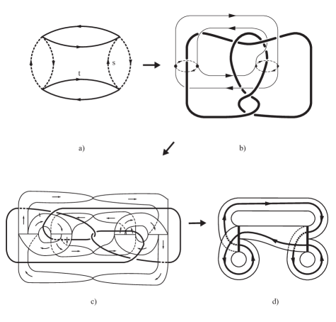
Figure 11: From random walks on the graph for the figure eight knot to dynamics on the universal template $\mathcal{T}$ of Ghrist

To deal with the fundamental group of the figure eight knot, Bowditch [$89$] extended theory of Markov triples to hyperbolic space H${}^{3}.$ To do so requires equations for Markov triples, eq.s(7.8), to be solved in the complex domain. In H³ the isometry group is PSL(2,C) as compared with the isometry group of H² which is PSL(2,R). As before, we can do all calculations using SL(2,C) and only at the end of calculations switch to PSL(2,C). Because of this,  it is useful to know [$90$] that SL(2,C) can be generated by just two elements

$$SL(2,\mathbf{C})=\{V=\left(\begin{array}[]{cc}1&\alpha\\ 0&1\end{array}\right),\hat{I}=\pm\left(\begin{array}[]{cc}0&-1\\ 1&0\end{array}\right),\alpha\in\mathbf{C}\}.$$ (7.33)

It is also helpful to compare these elements with earlier derived matrices $\hat{I}$ and $R$. Clearly, $V\rightarrow R$ when $\alpha\rightarrow 1.$In the case of figure eight knot it can be checked directly [$81$] that matrices $a$ and $b$ in eq.(7.31) can be presented as follows:

$$a=\left(\begin{array}[]{cc}1&1\\ 0&1\end{array}\right)\text{ and }b=\left(\begin{array}[]{cc}1&0\\ -\omega&1\end{array}\right),$$ (7.34)

where $\omega$ is one of the solutions of the equation $\omega^{2}+\omega+1=0.$ Typically, one chooses $\omega=\frac{1}{2}(-1+3i).$ This result has number-theoretic significance explained in the Appendix $B$ [$81$]. More deeply, theory of arithmetic hyperbolic 3-manifolds is explained in the book by [$91$]. Some physical (cosmological) implications of this arithmeticity are discussed in our work [$81$]. Interested readers are encouraged to read these references. By noticing that any matrix

$$SL(2,\mathbf{C})=\left(\begin{array}[]{cc}\alpha&\beta\\ \gamma&\delta\end{array}\right),\text{ \ }\alpha\delta-\gamma\beta=1\text{ }$$ (7.35)

can be represented in terms of $V$ and $\hat{I}$  as demonstrated in [$90$], it is clear that  now it is possible to represent all words in the form analogous to that given in eq.(7.26) or (7.27) (if the dihedral presentation, eq.(7.32), is used). Furthermore, the fundamental relation, eq.(7.13), for closed geodesics can be used for H³ also so that now we are dealing with the geodesic hyperbolic knots. The difference between the complements of the trefoil and that for figure eight knots lies in the fact that now the length $l$($\gamma)$ of geodesics becomes a complex number. It can be demonstrated [$89$], page 717, that Re$l$($\gamma)>0.\vskip 12.0pt plus 4.0pt minus 4.0pt$

Remark 7.6. Although the dihedral presentation is given in [$85$] incorrectly, it is possible to prove [$90$] that the finite subgroups of PSL(2,C) contain all group of orientation-preserving isometries of Euclidean regular solids and their subgroups. Evidently, the presence of actual symmetries depends upon the values of complex parameters $\alpha,\beta,\gamma,\delta$. The choice of D₂ leads to the universal template of Ghrist.

Remark 7.7. Instead of the real hyperbolic space H³ in which the complement of the figure eight knot lives, it is possible to use the complex hyperbolic space H${}_{\mathbf{C}}^{3}$ advocated by Goldman [$92$]. It is possible to consider a complement of the figure eight in H${}_{\mathbf{C}}^{3}$ as well [$93$]. It happens that isometry group of the boundary of H${}_{\mathbf{C}}^{3}$ is the Heisenberg group, e.g. see eq.s(6.14). Thus, in dealing with problems related to the complement of figure eight knot the contact geometry and topology again can be successfully used in accord with result obtained by Etnyre[$75$].

7.7. Cosmetic knots and gravity

Using results of part I, the famous Gordon and Luecke theorem [$72$] stating that in $S^{3}$ knots are determined by their complements can be restated now in physical terms. For this we need to recall some facts from general relativity. The original formulation by Einstein makes heavy emphasis on study of the Schwarzschild solution of Einstein’s equations originating from the Einstein field equations without sources with prescribed (spherical) symmetry in which the test mass enters as an adjustable parameter [$94$]. Using these equations the curvature tensor is obtained. If masses are associated with knots, then knot complements producing curved spaces around knots can be used for parametrizing the masses. In which case the Gordon and Luecke theorem is telling us that the mass spectrum is discrete.  In studying knotted geodesics in the complement of the trefoil and figure eight knot we followed Einsteinian methodology without recognizing Einsteinian influence. Indeed, we completely ignored the fact that each nontrivial knot in the complement of the trefoil/figure eight knot creates its own complement. Thus, the space around, say, the trefoil knot is not just a complement of the trefoil knot but it is the space made out of complements of all knots existing in the trefoil knot complement! This fact is ignored  in calculations presented above. Therefore, these ”complementary” knots are, in fact, closed geodesics on the punctured torus. Very much like in Einsteinian theory of gravity the motion of the point-like objects whose mass is ignored is taking place along the geodesics around the massive body whose field of gravity is described by the Schwarzschild solution. To account for extended sizes of particles in both general relativity and Yang-Mills field theory  is always a great challenge, e.g. read page 97 of  [$6$]. In the case of knotted geodesics the effect of extended size (that is of finite thickness of a geodesic) is also a difficult problem which is not solved systematically as can be seen from  [$85$].

To be specific, we would like to talk about the complement of the figure eight knot $K_{8}$. We begin with $S^{3}\smallsetminus K_{8}.$ This is a hyperbolic manifold. Next, we drill in it a closed curve $c$ (a tube of finite thickness or, which is the same, a tubular neighborhood, e.g. see Fig.3a)) which is freely homotopic to some geodesic $\gamma$. Such closed curve forms a link with $K_{8}.$ When we remove the content of knotted/linked tube from $S^{3}\smallsetminus K_{8}$ we obtain a manifold which is complementary to the link $K_{8}\cup c$ and, if we are interested in computation of the hyperbolic volume of such hyperbolic link, the result is going to depend very sensitively on the tube thickness. Thus, indeed, we end up with the situation encountered in gravity. Furthermore, additional complications might arise because of the following.

The Gordon and Luecke theorem [$72$] was proven for $S^{3}$ only. In the present case, say, if we are dealing with $M=S^{3}\smallsetminus K_{8}$ , the knots $K_{i}$ $,i=1,2....,$ living  in $S^{3}\smallsetminus K_{8}$ also will have their complements, that is $M\diagdown K_{i}$ and, because of this, we arrive at the following

Question: Suppose in some 3-manifold $M$ (other than $S^{3})$ there are two knots $K_{1}$ and $K_{2}$ so that the associated complements are $M\smallsetminus K_{1}$ and $M\smallsetminus K_{2}$. By analogy with Fig.12 suppose that there is  a homeomorphism $h$:  $h$($M\smallsetminus K_{1})=(M\smallsetminus K_{2}).$ Will such a homeomorphism imply that $K_{1}=K_{2}?$

If the answer to this question is negative, this then would imply that different knots would have the same complement in $M$. If we are interested in attaching some physics to these statements then, we  should only look for situations analogous to those in $S^{3}.$ This means that all physical processes should be subject to selection rules (just like in quantum mechanics) making such degenerate cases physically forbidden.  Evidently, all these considerations about the selection rules presuppose that the degeneracy just described can be realized in Nature. And indeed, it can! This leads us to the concept of cosmetic knots.

Definition 7.8. Let $M$ be some 3-manifold (other than $S^{3}$ and $S^{2}\times S^{1})$ and $K$ be some non-trivial knot ”living” in $M.$ If performing Dehn surgery on $K$ results in the same manifold $M$, then, the pair $(M,K)$ is called cosmetic pair.

Remark 7.9. To perform Dehn surgery physically is not possible. However, one can imagine a situation when  there are two different knots $K_{1}\neq$ $K_{2}$ such that their complements $M-K_{1}$ and $M-K_{2}$ are homeomorphic while knots themselves are not. If such situation can be realized then, if we want to keep the knot-mass correspondence alive, one should impose selection rules which will forbid such  cosmetic states.

Following Mathieu [$95$], consider now several details. To begin, we  have to notice similarities between the operations of cabling as depicted in Fig.7 and Dehn surgery.  After reading the description related to Fig.7 in the main text and the Definition F.1.,  it is appropriate to consider some knot $K$ in $S^{3}$ so that its complement $S^{3}\smallsetminus K=M$ is some 3-manifold with boundary. Let $k$ and $k^{\prime}$ be the cores of the respective surgeries for this knot in $M$.  There should be a homeomorphism from $S^{3}\smallsetminus K$ to $M\smallsetminus k$ sending the curve $J$ (for $K$) onto meridian $\mathfrak{m}$ of $k.$ At the same time, there should be a homeomorphism from $S^{3}\smallsetminus K$ to $M\smallsetminus k^{\prime}$ sending another curve $\tilde{J}$ (for $K$) onto meridian $\mathfrak{m}^{\prime}$ of $k^{\prime}$. Should $k$ and $k^{\prime}$ be equivalent, then by using composition of mappings it would be possible to find a homeomorphism in $M=S^{3}\smallsetminus K$ -from $J$ to $\tilde{J}$ -without preserving the meridian of $K.$ Notice that, by design, $J$ $\neq$ $\pm\tilde{J}$ making such homeomorphism impossible. Therefore, $k$ and $k^{\prime}$ are not equivalent while the complements $M\smallsetminus k$ and $M\smallsetminus k^{\prime}$ are since they are homeomorphic.

Remark 7.10. Let $K$ be a trefoil knot. Then in its complement there will be cosmetic knots. In fact, all Lorenz knots are cosmetic. The same is true for all knots living in the complement of the figure eight knot. Evidently, such cosmetic knots cannot be associated with physical masses.

Appendix A.  The Beltrami equation and contact geometry

Consider 3-dimensional Euclidean space. Let A be some vector in this space so that $\mathbf{A}=\mathop{\displaystyle\sum}\nolimits_{i=1}^{3}A_{i}\mathbf{e}_{i}$ . Introduce next the $\flat-$operator via

$$\left(\mathbf{A}\right)^{\flat}=\mathop{\displaystyle\sum}\nolimits_{i=1}^{3}A_{i}dx_{i}.$$ (A.1)

Use of $\flat$ allows us now to write

$$d\left(\mathbf{A}\right)^{\flat}=(\frac{\partial A_{2}}{\partial x_{1}}-\frac{\partial A_{1}}{\partial x_{2}})dx_{1}\wedge dx_{2}+(\frac{\partial A_{1}}{\partial x_{3}}-\frac{\partial A_{3}}{\partial x_{1}})dx_{3}\wedge dx_{1}+(\frac{\partial A_{3}}{\partial x_{2}}-\frac{\partial A_{2}}{\partial x_{3}})dx_{2}\wedge dx_{3}$$ (A.2)

Next, we obtain,

$$\ast d\left(\mathbf{A}\right)^{\flat}=(\frac{\partial A_{2}}{\partial x_{1}}-\frac{\partial A_{1}}{\partial x_{2}})dx_{3}+(\frac{\partial A_{1}}{\partial x_{3}}-\frac{\partial A_{3}}{\partial x_{1}})dx_{2}+(\frac{\partial A_{3}}{\partial x_{2}}-\frac{\partial A_{2}}{\partial x_{3}})dx_{1}.$$ (A.3)

Finally, by using an inverse operation to $\flat$ we obtain,

$$\left[\ast d\left(\mathbf{A}\right)^{\flat}\right]^{\natural}=(\frac{\partial A_{2}}{\partial x_{1}}-\frac{\partial A_{1}}{\partial x_{2}})\mathbf{e}_{3}+(\frac{\partial A_{1}}{\partial x_{3}}-\frac{\partial A_{3}}{\partial x_{1}})\mathbf{e}_{2}+(\frac{\partial A_{3}}{\partial x_{2}}-\frac{\partial A_{2}}{\partial x_{3}})\mathbf{e}_{1}=curl\mathbf{A.}$$ (A.4)

Using these results we obtain as well

$$\ast d\left(\mathbf{A}\right)^{\flat}=\left(\mathbf{\nabla}\times\mathbf{A}\right)^{\flat}.$$ (A.5)

If $\left(\mathbf{A}\right)^{\flat}=\alpha,$ where $\alpha$ is contact 1-form,  then the Beltrami equation reads as

$$\ast d\alpha=\kappa\alpha.$$ (A.6)

Appendix B.  Derivation of the force-free equation from the source-free Maxwell’s equations

In Appendix 4 of part I we mentioned about works by Chu and Ohkawa [$96$] and Brownstein [$97$] in which the force-free equation is derived from the source-free Maxwell’s equations. In this appendix we use some results from the paper by Uehara, Kawai and Shimoda [$98$] in which the same force-free equation was obtained in the most transparent way. In the system of units in which $\varepsilon_{0}=\mu_{0}=1$ the source-free Maxwell’s equations acquire the following form

$$\frac{\partial}{\partial t}\mathbf{E}=\mathbf{\nabla}\times\mathbf{B}\text{ \ and \ }-\frac{\partial}{\partial t}\mathbf{B}=\mathbf{\nabla}\times\mathbf{E,}$$ (B.1)

provided that div$\mathbf{B}=$div$\mathbf{E}=0.$ Let $\mathbf{E}=\mathbf{v}(\mathbf{r},t)\cos f(\mathbf{r},t)$ and $\mathbf{B}=\mathbf{v}(\mathbf{r},t)\sin f(\mathbf{r},t)$. In view of the fact that $\mathbf{\nabla}\times(a\mathbf{v})=a\mathbf{\nabla}\times\mathbf{v}-\mathbf{v\times\nabla}a$  use of E and B in Maxwell’s equations leads to the following results

$$-\dot{f}\mathbf{v}\sin f+\mathbf{\dot{v}}\cos f=\sin f(\nabla\times\mathbf{v})-\left(\mathbf{v\cdot\nabla}f\right)\cos f$$ (B.2a)

and

$$\dot{f}\mathbf{v}\cos f+\mathbf{\dot{v}}\sin f=-\cos f(\nabla\times\mathbf{v})-\left(\mathbf{v\cdot\nabla}f\right)\sin f$$ (B.2b)

where, as usual, the dot $\cdot$ over $f$ denotes time differentiation. Analysis shows that eq.(B.2a) and (B.2b) equivalent to the following set of equations

$$\dot{f}\mathbf{v=-\nabla\times v}$$ (B.3a)

and

$$\mathbf{\dot{v}}=-\mathbf{v\times\nabla}f$$ (B.3b)

while the incompressibility equations div$\mathbf{B}=$div$\mathbf{E}=0$ are converted into the requirements

$$\text{div}\mathbf{v}=0$$ (B.4a)

and

$$\mathbf{v}\cdot\nabla f=0.$$ (B.4b)

If now we identify $\mathbf{v}$ with the fluid velocity, then both eq.s(B.4a) and (B.4b) can be converted into one equation div$(f\mathbf{v})=0$ which we had encountered already in section 4 of part I. E.g. read the text below the eq.(4.3). This observation allows us to reinterpret eq.s(B.3a) and (B.3b). Specifically, if we let $\dot{f}=-\kappa(\mathbf{r})$ in eq.(B.3a), then the force-free equation

$$\mathbf{\nabla\times v=}\kappa\mathbf{v}$$ (B.5)

is obtained. By  applying the curl operator to both sides of this equation and taking into account eq.(B.4a) we obtain

$$-\nabla^{2}\mathbf{v=}\kappa^{2}\mathbf{v}+\left(\mathbf{\nabla}\kappa\right)\times\mathbf{v.}$$ (B.5)

Now eq.(B.3b) can be rewritten as $\mathbf{\dot{v}}=t(\mathbf{v\times\nabla}\kappa).$This result can be formally used in eq.(B.5). The Hemholtz equation

$$\nabla^{2}\mathbf{v+}\kappa^{2}\mathbf{v=}0$$ (B.6)

is obtained if $\left(\mathbf{\nabla}\kappa\right)\times\mathbf{v=}0$. Since in addition $\kappa$ must also satisfy eq.(B.4b), we conclude that $\kappa=const$ is the only admissible solution. As discussed in [$6$], the Helmholtz eq.(B.6) is related to the force-free eq.(B.5)  as the Klein-Gordon equation is related to the Dirac equation. This means that every solution of eq.(B.5) is also a solution of eq.(B.6) but not another way around.

Using just obtained results, the energy density, eq.(2.11) of part I, manifestly time-independent. In the non-Abelian case of Y-M fields this would correspond to the case of monopoles in accord with statements made in part I.

Consider now briefly the case when  v is time-depemdent. Then eq.(B.5) can be equivalently rewritten as

$$\mathbf{\dot{v}=-}t\mathbf{(}\nabla^{2}\mathbf{v+}\kappa^{2}\mathbf{v).}$$ (B.7)

Let now v(r,t) =V(r)T(t). Using this result in eq. (B.7) we obtain

$$\frac{-1}{tT(T)}\dot{T}(t)=\frac{1}{\mathbf{V}}(\nabla^{2}\mathbf{V+}\kappa^{2}\mathbf{V).}$$ (B.8)

If $\ \nabla^{2}\mathbf{V+}\kappa^{2}\mathbf{V=-}E\mathbf{V},$ then the Helmholtz eq.(B.6) should be replaced by the same type of equation in which we have to make a substitution $\kappa^{2}$ $\rightarrow\kappa^{2}+E=\mathcal{K}^{2}$ and then to treat $\mathcal{K}^{2}$ as an eigenvalue  of thus modified eq.(B.6) with the same boundary conditions, e.g.  see eq.(2.1b). The situation in the present case is completely analogous that for  the Navier-Stokes equation, e.g. read Majda and Bertozzi [$22$],Chr.2. Therefore, the solution $\mathbf{v}(\mathbf{r},t)=\mathbf{V}(\mathbf{r})T(t)$ of the Navier-Stokes equation is represented as the Fourier expansion over the egenfunctions of the force-free (or Beltrami) eq.(B.5) $\mathbf{V}(\mathbf{r})\rightarrow\mathbf{V}_{m}(\mathbf{r})$. Using eq.(B.8) $T(t)$ is straightforwardly obtainable. By applying the appropriate reparametrization $T(t)$ can be brought to the form (e.g. see eq.(3.8) of part I and comments next to it) suggested by Donaldson [$99$]. Thus, even in the case of time-dependent solutions  the obtained results can be made consistent with  those suggested by Floer and Donaldson which were discussed in part I. Because of this, it is sufficient to treat only the time-independent case. In electrodynamics this corresponds to use of the constant electric and magnetic transversal fields.

Appendix C  Some facts from symplectic and contact geometry

Consider a symplectic 2-form $\omega=\mathop{\displaystyle\sum}\nolimits_{j=1}^{m}dp_{j}\wedge dq_{j}.$ Introduce a differentiable function $f^{(\mathbf{v})}$ associated with the vector field $\mathbf{v}$  via skew-gradient

$$\mathbf{v}=(sgrad)f^{(\mathbf{v})}=\mathop{\displaystyle\sum}\nolimits_{i}[\frac{\partial f^{(\mathbf{v})}}{\partial p_{i}}\frac{\partial}{\partial q_{i}}-\frac{\partial f^{(\mathbf{v})}}{\partial q_{i}}\frac{\partial}{\partial p_{i}}]$$ (C.1a)

and such that $-df^{(\mathbf{v})}=i_{\mathbf{v}}\omega$. This  result can be checked by direct computation. By definition, a vector field $\mathbf{v}$ is symplectic if $\mathcal{L}_{\mathbf{v}}\omega=0.$ Since $\mathcal{L}_{\mathbf{v}}=d\circ i_{\mathbf{v}}+i_{\mathbf{v}}\circ d$ , we obtain: $\mathcal{L}_{\mathbf{v}}\omega=-ddf^{(\mathbf{v})}=0,$ as required. Introduce now another  vector field $\mathbf{w}$ via

$$\mathbf{w}=(sgrad)f^{(\mathbf{w})}=\mathop{\displaystyle\sum}\nolimits_{i}[\frac{\partial f^{(\mathbf{w})}}{\partial p_{i}}\frac{\partial}{\partial q_{i}}-\frac{\partial f^{(\mathbf{w})}}{\partial q_{i}}\frac{\partial}{\partial p_{i}}]$$ (C.1b)

and calculate $i_{\mathbf{w}}\circ i_{\mathbf{v}}\omega.$ We obtain:

$$i_{\mathbf{w}}\circ i_{\mathbf{v}}\omega = i_{\mathbf{w}}(-df^{(\mathbf{v})})=i_{\mathbf{w}}\mathop{\displaystyle\sum}\nolimits_{i}(-\frac{\partial f^{(\mathbf{v})}}{\partial p_{i}}dp_{i}-\frac{\partial f^{(\mathbf{v})}}{\partial q_{i}}dq_{i})=\mathop{\displaystyle\sum}\nolimits_{i}[\frac{\partial f^{(\mathbf{v})}}{\partial p_{i}}\frac{\partial f^{(\mathbf{w})}}{\partial q_{i}}-\frac{\partial f^{(\mathbf{v})}}{\partial q_{i}}\frac{\partial f^{(\mathbf{w})}}{\partial p_{i}}]$$ (55)

$$\equiv \{f^{(\mathbf{v})},f^{(\mathbf{w})}\}=\omega(\mathbf{v},\mathbf{w})=\mathbf{v}f^{(\mathbf{w})}=-\mathbf{w}f^{(\mathbf{v})}.\TCItag{C.2}$$

The combination $\{f^{(\mathbf{v})},f^{(\mathbf{w})}\}$ is instantly recognizable as the Poisson bracket. Let now $f^{(\mathbf{v})}=H,$ where $H$ is the Hamiltonian, then $-dH=i_{\mathbf{v}}\omega$ $=-\mathop{\displaystyle\sum}\nolimits_{i}(\dfrac{\partial H}{\partial q_{i}}dq_{i}+\dfrac{\partial H}{\partial p_{i}}dp_{i})$ as required. At the same time, since $\dfrac{\partial H}{\partial q_{i}}=-\dot{p}_{i}$ and $\dfrac{\partial H}{\partial p_{i}}=\dot{q}_{i}$ we can rewrite eq.(C.1a) as

$$\mathbf{v}_{H}=(sgrad)H=\mathop{\displaystyle\sum}\nolimits_{i}[\dot{q}_{i}\frac{\partial}{\partial q_{i}}+\dot{p}_{i}\frac{\partial}{\partial p_{i}}].$$ (C.1c)

By design, we obtain then $dH(\mathbf{v}_{H})=0$.

Appendix D  Some facts about the Morse-Smale flows

Let $\mathcal{M}$ be some smooth $n-$dimensional manifold. To describe the motion on $\mathcal{M}$  we associate with each $t\in\mathbf{R}$  (or R${}^{+})$ a mapping $g^{t}:\mathcal{M}\rightarrow\mathcal{M}$ -a group (semigroup) of diffeomorphisms with the property $g^{t+s}=g^{t}g^{s},g^{0}=\mathbf{1}_{M}.$ For some $\mathbf{x}\in\mathcal{M}$ suppose that some point-like particle was initially located at $\mathbf{x}$. Then after time $t$ the (phase)flow (trajectory) will carry this particle to $g^{t}\mathbf{x}$ so that the velocity $\mathbf{v}(\mathbf{x})=\frac{d}{dt}\mid_{t=0}g^{t}\mathbf{x}.$ The function $t\longrightarrow g^{t}\mathbf{x}$ is called the motion. In physics this is written as $\mathbf{\dot{x}}=\mathbf{v}(\mathbf{x}).$ This is a system of ordinary differential equations. It is supplemented by the initial condition $\mathbf{x}(0)=\mathbf{x}_{0}.$ The vector $\mathbf{v}(\mathbf{x})$ belongs to the tangent space of $\mathcal{M}$ at $\mathbf{x}$, that is $\mathbf{v}(\mathbf{x})\in T_{x}\mathcal{M}.$ Sometimes it happens that $g^{t}\mathbf{\tilde{x}=\tilde{x}}$ $\forall t.$ Such point $\mathbf{\tilde{x}}$ is called the equilibrium point. Otherwise, there could be some (period) $T$ such that $g^{t+T}\mathbf{\tilde{x}=\tilde{x}.}$ In this case the point $\mathbf{\tilde{x}}$ is called periodic. It belongs to the periodic (closed) trajectory. Suppose now that we are having another manifold $\mathcal{N}$  so that there is a map (a homomorphism) $h:\mathcal{M}\rightarrow\mathcal{N}.$ Dynamical systems (flows) $g^{t}$on $\mathcal{M}$ and $\check{g}^{t}$on $\mathcal{N}$ are topologically conjugate if $h\circ g^{t}=\check{g}^{t}\circ h.$ With the topological conjugacy associated structural stability. Omitting some fine details which can be found, for example, in Arnol’d [$100$], we shall not be making distinctions between topological conjugacy and structural stability.

The analysis of the flow described by $\mathbf{\dot{x}}=\mathbf{v}(\mathbf{x})$  begins with linearization. For this purpose we select some point $\mathbf{\tilde{x}}$ along the trajectory. Typically such a point is the equilibrium point. Let $\mathbf{x}=\mathbf{\tilde{x}+x-\tilde{x}\equiv\tilde{x}+\delta x.}$ Using this result in $\mathbf{\dot{x}}=\mathbf{v}(\mathbf{x})$ we obtain

$$\mathbf{\delta}\dot{x}_{i}\text{{=}}\mathop{\displaystyle\sum}\limits_{j}\frac{\partial v_{i}}{\partial x_{j}}\mid_{\mathbf{x}=\mathbf{\tilde{x}}}\delta x_{j}.$$ (D.1)

The equilibrium point $\mathbf{\tilde{x}}$ is called hyperbolic if all the eigenvalues of the matrix $A_{ij}=\frac{\partial v_{i}}{\partial x_{j}}\mid_{\mathbf{x}=\mathbf{\tilde{x}}}$ are real (that is not complex). It is called nondegenerate if all eigenvalues are nonzero. Since eq.(D.1) is in $T\mathcal{M}$ space it is clear that replacing Rⁿ by $\mathcal{M}$ and vice versa introduces nothing new into local study of the system of equations $\mathbf{\dot{x}}=\mathbf{v}(\mathbf{x}).$ The question of central importance is the following. How can solution of eq.(D.1) help us in solving equation $\mathbf{\dot{x}}=\mathbf{v}(\mathbf{x})?$ The answer is given by the following

[$101$]

Theorem D.1. (Grobman -Hartman) If the point $\tilde{x}$ is hyperbolic, then there is a homeomorphism defined on some neighborhood U of $\tilde{x}$ in Rⁿ locally taking orbits of the nonlinear flow $g^{t}$ to those of linear flow defined by $exp(tA_{ij}).$

The above theorem is being strengthened by the following

Theorem D.2. Suppose that equation $\mathbf{\dot{x}}=\mathbf{v}(\mathbf{x})$ has a hyperbolic fixed point $\mathbf{\tilde{x}}$. Then there exist local stable and unstable manifolds $W^{s}(\mathbf{\tilde{x}}),W^{u}(\mathbf{\tilde{x}})$ of the same dimensions $d_{s}=d_{u}$ as those of eigenspaces $E^{s}$ ($\lambda_{l}\mathop{\mathrm{n}egative})$ and $E^{u}(\lambda_{l}$ positive), $\lambda_{l}$ are eigenvalues of the matrix $A_{ij}.$ $W^{s}(\mathbf{\tilde{x}})$ and $W^{u}(\mathbf{\tilde{x}})$ are tangent to $E^{s}$ and $E^{u}$ respectively.

Remark D.3. Eigenspaces $E^{s}$ and $E^{u}$ are made of respective eigenvector spaces. As in quantum mechanics, it is possible to make egenvectors mutually orthogonal. If this is possible, the associated stable and unstable manifolds are transversal to each other. These manifolds are considered to be transversal to each other even when the associated eigenvectors are not orthogonal (since they can be made orthogonal). The existence and uniqueness of the solution of $\mathbf{\dot{x}}=\mathbf{v}(\mathbf{x})$ ensures that two stable/unstable manifolds of distinct fixed points, say $\mathbf{\tilde{x}}_{1}$ and $\mathbf{\tilde{x}}_{2},$ cannot intersect. For the same reason $W^{s}(\mathbf{\tilde{x}})$ and $W^{u}(\mathbf{\tilde{x}})$ cannot self-intersect. However, intersections of stable  and unstable manifolds of distinct fixed points or even of the same fixed point are allowed. To define the Morse-Smale flows we need to introduce the following.

Definition D.4. A point $p$ is called nonwandering for the flow $g^{t}$ if  for any

neighborhood $U$ of $p$  there exists arbitrary large $t$ such that $g^{t}(U)$ $\cap U\neq\varnothing$ .

From here it follows, in particular, that fixed points and periodic orbits are non wandering.

Definition D.5. A Morse-Smale dynamical system is the one for which

the following holds.

1. The number of fixed points and periodic orbits is finite and each is hyperbolic.

2. All stable and unstable manifolds intersect transversely.

3. The non wandering set consists of fixed points and periodic orbits alone.

Corollary D.6. The Morse- Smale systems are structurally stable. Furthermore,

compact manifolds can possess only a finite number of periodic orbits and fixed points.

Definition D.7. The nonsingular Morse-Smale flow (NMS) does not contain fixed points.

Corollary D.8. The Poincar$e^{\prime}$-Hopf index theorem permits NMS flow only on manifolds

whose Euler characteristic is zero. Therefore, such flows cannot

be realized, say, on $S^{2}$ but can be realized on $T^{2}.$ On $S^{3}$ such flows also can exist.

Details are discussed in the main text.

Appendix E     Some basic facts about Seifert fibered spaces

A Seifert fibered manifold $M$ is a fiber bundle $(M,N,\pi,S^{1})$ with $M$ being the total space, $N$ being the base, called the orbit manifold/orbit space. Typically, it is an orbifold, that is the manifold with corners/cones). $\pi$ is the projection, $\pi:M\rightarrow N,$ and $S^{1}$ is the fiber.  Let $\mathcal{F}$ be one of such fibers. A Seifert fibered manifold is characterized by the property that each $\mathcal{F}$  has a fibered neighborhood  which can be mapped into a fibered solid torus.  It is made out of a fibered cylinder $D^{2}\times I$ in which the fibers are $x\times I,$ $x\in D^{2}.$ By rotating $D^{2}\times I$ through the angle $2\pi$ ($\nu/\mu)$ while keeping $D^{2}\times 0$ fixed and identifying $D^{2}\times 0$ with $D^{2}\times I$ a fibered solid torus is obtained. Upon such an identification  the fibers of $D^{2}\times I$ are being decomposed into classes in such a way that each class contains exactly $\mu$ lines which match together to give one fiber of the solid torus, e.g. see Fig.4a), except that which is belonging to the class containing the axis of $D^{2}\times I.$ This fiber remains unchanged after identification. It belongs to the class called singular (exceptional, middle)  [$56$] . When $\mu=1$ the fiber bundle (still  to be constructed) is trivial. The number $\mu$ is called multiplicity of the singular fiber. There always exist a fiber-preserving homeomorphism into fibered solid torus such that $\mathcal{F}$ can be mapped into a singular fiber. Reciprocally, from this property it follows that each fibered neighborhood of $\mathcal{F}$ should have a boundary. Naturally, it should be $T^{2}.$ This means that there should be a homeomorphism placing $\mathcal{F}$ onto $T^{2}$ in the form of some closed curve $J$. Such a curve is being defined by its meridian $\mathfrak{M}$ and longitude $\mathfrak{L.}$ The longitude $\mathfrak{L}$ of the solid torus is a simple closed curve on $T^{2}$ which intersects $\mathfrak{M}$  in exactly one point.  Thus formally, we can write

$$J\sim\nu\mathfrak{M}+\mu\mathfrak{L.}$$ (E.1a)

The numbers $\nu$ and $\mu$ are the same for all fibered neighborhoods of $\mathcal{F}$. Furthermore, from the way the solid torus was constructed, it easily follows that the number $\nu$ is defined not uniquely: $\nu_{1}=\nu_{2}$ $\left(\mathop{\mathrm{m}od}\mu\right).$ Therefore fibrations $2\pi$ ($\nu/\mu)$ and $2\pi$ ($\nu+n\mu/\mu)$ are indistinguishable. In view of previous results,  we shall call the nonsingular   fiber $\mathcal{F}$ for $\mu>1$ as regular.  The following theorem is of central importance

Theorem E.1. A closed (compact) Seifert fibered space contains at most finitely many singular fibers.

From here it follows that all singular fibers are isolated. It is possible to design Seifert manifolds without singular fibers though. In view of their importance, we briefly sketch their design. Let $N$  be an orbit space. Suppose that it is a compact orientable surface with non-empty boundary  (made of $\partial D_{i}^{2}$ , $i=1,...,n).$ Then $M=N\times S^{1}$ is a Seifert fibered manifold (a trivial fiber bundle) with fibers $x\times I,$ $x\in N.$ An orientable saddle, Fig.3a), defined in section 5 is an example of such manifold.

Using thus designed (nonsingular) Seifert manifold, it is possible now to design a manifold with singular fibers. For this purpose we select $n$ pairs of coprime integers $(\alpha_{i},\beta_{i}),$ then we select a base $N$ which  we had already described. It is a compact orientable surface from which $n$ open discs $\mathring{D}_{i}^{2}=D_{i}^{2}$ $\smallsetminus\partial D_{i}^{2}$ are removed so that the obtained surface $\tilde{N}=N-(\mathring{D}_{1}^{2}\cup\cdot\cdot\cdot\cup\mathring{D}_{n}^{2}).$ By design, such Seifert manifold $\tilde{M}=\tilde{N}\times S^{1}$ is Seifert manifold without singular fibers. Because of Theorem E.1. it is appropriate to associate the locations of singular fibers with the locations of the discs $D_{i}^{2}.$  By doing so we are going to construct a Seifert manifold with singular fibers. For this purpose we need to notice that with the boundary $\partial D_{i}^{2}$ of each disc $i$ the map $\pi^{-1}(\partial D_{i}^{2})\rightarrow T_{i}^{2}$ can be associated. Choose on $T_{i}^{2}$ the meridian $\mathfrak{M}_{i}=\partial D_{i}^{2}\times\{\ast\}$ and the longitude $\mathfrak{L}_{i}=\{\ast\}_{i}\times S^{1}$ consistent with the orientation of $\tilde{M}.$ At the boundary $\partial D_{i}^{2}\times S^{1}=$ $T_{i}^{2}$ we can construct a curve $J_{i}$ of the same type as given by eq.(E.1a)

$$J_{i}\sim\alpha_{i}\mathfrak{M}_{i}+\beta_{i}\mathfrak{L}_{i}$$ (E.1b)

(we use the pair $(\alpha_{i},\beta_{i})$ for its description). Take now trivially fibered solid torus $D^{2}\times S^{1}$and glue it to $T_{i}^{2}$ in such a way that its meridian $\mathfrak{\tilde{M}}_{i}$ is glued to $J_{i}\in T_{i}^{2}.$ For each $i$ the image under gluing of the curve $\{0\}\times S^{1}\in D^{2}\times S^{1}$ is going to become the i-th singular fiber. This gluing homeomorphism is the last step in designing the Seifert fibered manifold with $n$ singular fibers. A particular Seifert fibered manifold can be now described via the following specification: $M=M(N;(\alpha_{1},\beta_{1}),...,(\alpha_{n},\beta_{n})).$ In section 5 an example of such a manifold is given by the non-orientable saddle, e.g. see Fig.4a). It is the Seifert fibered manifold of the type $M=M(D^{2};(2,1))$ with one singular fiber. Incidentally, if the orbit manifold is $S^{2}$, then the obtained Seifert manifold  is already familiar Hopf fibration. It is a Seifert fibered manifold without singular fibers [$71$], page 87. Other Seifert-fibered manifolds without singular fibers having $S^{2}$ as their orbit space are $S^{2}\times S^{1}$ and the Lens spaces of the type $L(n,1)$. For $n=1$ we get back the Hopf fibration, for $n=2$ we get the projective space P³, while the $n=0$ case is identified with $S^{2}\times S^{1}.$ Finally, a complement of any torus knot in $S^{3}$ is Seifert fibered space too [$71$], page 87.

Appendix F Some facts about Kirby moves/calculus

In the famous theorem by Gordon and Luecke [$72$] it is proven that knots are determined by their complements. That is to say, a non-trivial Dehn surgery on a non-trivial knot in $S^{3}$ does not yield back $S^{3}$. This theorem does not cover the case of links as Fig.12 illustrates.

Figure 12: The generic case (Rolfsen1976), page 49, of generating topologically different links having the same complement in $S^{3}$

In section 7.7 we argued that the theorem by Gordon and Luecke [$72$] could be also violated for the case of  some knots. In Fig.12 the initial state is a). It is made out of two unknots (e.g. think also about the Hopf link). The final state is d). To reach d) from a) we have to perform a reversible homeomorphism- from b) to c). The trick is achieved by enclosing the original link located in $S^{3}$ into a solid torus, just like it is done in the case of Fig.3a), and then performing the Dehn twist (or the sequence of Dehn twists). This is further illustrated in going from c) to f).

This generic example can be extended in several directions. For instance, one of these directions was developed by Robion Kirby [$102$]. He invented moves, now known as Kirby moves/calculus, broadly generalizing situation depicted in Fig.12. To explain what he did we have to introduce several definitions. We begin with

Definition F.1.(Dehn surgery) Let $K$ be some knot in some 3-manifold $M$. Let $N(K)$ be a tubular neighborhood of $K$ (that is trivially fibered (that is without a twist) solid torus). Remove now this solid torus $N(K)$ from $M.$ Then, what is left is a 3-manifold with boundary $\mathring{M}=M\smallsetminus intN(K)$ where int means ”interior” and the solid torus $N(K)=$ $D^{2}\times S^{1}.$ $\mathring{M}$ is the manifold whose boundary is $T^{2}$ that is $\partial\mathring{M}=T^{2}.$ Apparently, $M=\mathring{M}\cup(D^{2}\times S^{1}).$ To complicate matters we can glue the solid torus back into $\mathring{M}$ via some homeomorphism $h:\partial D^{2}\times S^{1}\rightarrow T^{2}.$ In such a case, instead of $M=\mathring{M}\cup(D^{2}\times S^{1}),$ we obtain $\tilde{M}=\mathring{M}\cup_{h}(D^{2}\times S^{1}).$ Thus, a 3-manifold $\tilde{M}$  is obtained from $M$ via Dehn surgery along $K.\vskip 12.0pt plus 4.0pt minus 4.0pt$

The manifold $\tilde{M}$ depends upon the specification of $h$. It can be demonstrated that it is sufficient to use the following type of (gluing) homeomorphism. Choose $J\sim\alpha\mathfrak{M}+\beta\mathfrak{L}$ at the boundary $T^{2}$ of $\mathring{M}.$ Let $\mathfrak{M}$ be the meridian $\partial D^{2}\times\{\ast\}$ of the solid torus $N(K).$ Then the $h$ is defined by the map: $J=h(\partial D^{2}\times\{\ast\}).\mathop{\mathrm{S}i}$nce the pairs $(\alpha,\beta)$ and $(-\alpha,-\beta)$ define the same curve $J$, it is clear that the ratio $r=$ $\alpha/\beta$ determines $J$.  In particular, since $1/0=\infty$ determines the meridian, the result of any $1/0$ surgery leaves $M$ unchanged. Incidentally, the surgery determined by $r=0$ along the trivial knot switchers meridian with parallel (the torus switch). This type of surgery leads to the 3-manifold $S^{2}\times S^{1}$. The types of surgeries determined by the rational $r$ are called rational. The surgery is integral if $\beta=\pm 1.$ As demonstrated by Lickorish and Wallace [$54$] any closed orientable 3-manifold can be obtained by an integral surgery along a link $\mathcal{L}\subset S^{3}.\vskip 12.0pt plus 4.0pt minus 4.0pt$

Remark F.2. Operation of Dehn surgery is technically closely related to the cabling operation, e.g. see Fig.7.

Definition F.3. The procedure of  assigning of $r_{i}$ for each component $\mathcal{L}_{i}$ of $\mathcal{L}$ is called framing.

It is very helpful to think about the integral surgery/framing in terms of linking numbers. The linking number  for oriented knots/links can be easily defined via knot/link projection. Using the convention as depicted in Fig.13

Figure 13: The sign convention used for calculation of a) linking and b) sel-linking (writhe) numbers for oriented links (for a) and knots (for b) respectively

the linking number lk($L_{1}$,$L_{2})$ for oriented curves(links) $L_{1}$and $L_{2}$ is defined as

$$lk(L_{1},L_{2})=\mathop{\displaystyle\sum}\limits_{i}\varepsilon_{i}\text{, \ }\varepsilon=\pm 1.$$ (F.1)

Evidently, $lk(L_{1},L_{2})=lk(L_{2},L_{1})$ and $lk(-L_{1},L_{2})=-lk(L_{2},L_{1})$. Here $-L_{1}$ means link $L_{1}$ with orientation reversed.

Notice now that in the case of integral surgery the meridian $\mathfrak{M}$ is being mapped into the curve $J=\alpha\mathfrak{M}+\mathfrak{L.}$ From here it follows that $J$ is making exactly one revolution in the direction parallel to $\mathfrak{L}$. Locally this situation can be illustrated with help of a ribbon depicted in Fig.14a).

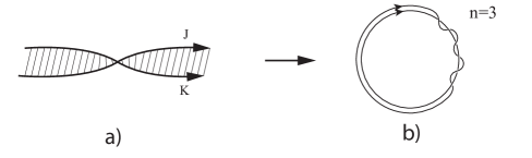
Figure 14: Example of framing

From here we obtain the following

Definition F.4.  The integral framing of a knot $K$ corresponds to the choice $lk(K,\mathfrak{L})=\alpha=n,$ where $n$ is an integer. An example of integral framing is depicted in Fig.14b). In appendix E it was stated that both Hopf links and complements of any torus knots in $S^{3}$ are Seifert fibered spaces. This does not mean  that  these spaces  must be the same.  Following Lickorish and Wallace [$51,54$], we can construct these Seifert fibered 3-manifolds using some sequence of  integral surgeries.  This brings us to

The main question: (Kirby) How to determine when two differently framed  links  produce the same 3-manifold?

The answer to this question is given in terms of two (Kirby) moves. They are designed as equivalence relations between links with different framings which produce the same 3-manifolds. It is possible to inject some physics into these equivalence moves using results of part I. Specifically, following conventions, the value of integral framing is depicted next to the respective projection of knot/link. For instance, if we supply the framing $\pm 1$ to the unknot, it is becoming the Hopf link. It was identified in part I with the magnetic or electric charge. Accordingly, the 1st Kirby move depicted in Fig.15 represents the charge conservation (e.g. see Fig.8).

Figure 15: The fist Kirby move

This move can be interpreted as follows: It is permissible to add or delete an unknot with framing $\pm 1$ which does not intersect the other components of $\mathit{L}_{i}$ to a given link $\mathcal{L}$. The 2nd Kirby move is depicted in Fig.16.

Figure 16: The second Kirby move

Physically, it can be interpreted  in terms of interaction between charges.  Mathematically this move can be interpreted as follows. Let $L_{1}$ and $L_{2}$ be two link components framed by the integers $n_{1}$ and $n_{2}$ respectively and $L_{2}^{\prime}$ a longitude defining the framing of $L_{2}$ that is $lk(L_{2},L_{2}^{\prime})=n_{2}.$ Replace now the pair $L_{1}$ $\cup$ $L_{2}$ by another pair $L_{1\#}$ $\cup$ $L_{2}$ in which $L_{1\#}=L_{1}$ $\#_{b}$ $L_{2}^{\prime}$ and $b$ is 2-sided band connecting $L_{1}$ with $L_{2}^{\prime}$ and disjoint from another link components. While doing so, the rest of the link $\mathcal{L}$ remains unchanged. The framings of all components, except $L_{1},$ are preserved while the framing of $L_{1}$ is being changed into that for $L_{1\#}$ and is given by $n_{1}$ $+$ $n_{2}+2lk(L_{1},L_{2}).$ The computation of $lk(L_{1},L_{2})$ proceeds in the standard way as described above (e.g. see Fig.13), provided that both $L_{1}$ and $L_{2}$ are oriented links.

Remark F.5. Using the 1st and the 2nd Kirby moves it is possible now to extend/improve results depicted in Fig.12. These improvements are summarized and depicted in Fig.17.

Figure 17: The Kirby moves, operations a) and b), are called ”blow down” for arrows pointing to the right, and ”blow up” for arrows pointing to the left. Twistings on the r.h.s. are known as the Fenn-Rourke moves.These can be used instead of Kirby moves

The Fenn-Rourke moves are equivalent to blow ups /downs and are equivalent to the combined first and second Kirby-type moves [$51$].

Remark F.6. By comparing Kirby moves just described against those suggested by Wada [$50$](e.g. see Fig.s 2-7 of paper by Campos et al [$61$]) it is clear that the moves suggested by Wada are just specific adaptations of Kirby (or Fenn-Rourke) moves.

Appendix G Calculations of the various presentations for the fundamental

group of the figure eight knot

a) We begin with the set of relations

$$r_{1}:bcb^{-1}=a,\rightarrow c=b^{-1}ab$$ (G.1)

$$r_{2}:ada^{-1}=b,\rightarrow d=a^{-1}ba$$ (G.2)

$$r_{3}:d^{-1}bd=c,\rightarrow\left(a^{-1}ba\right)^{-1}b\left(a^{-1}ba\right)=c=b^{-1}ab$$ (G.3)

$$r_{4}:c^{-1}ac=d\rightarrow\left(b^{-1}ab\right)^{-1}a(b^{-1}ab)=d=a^{-1}ba$$ (G.4)

Noticing now that $\left(a^{-1}ba\right)^{-1}=a^{-1}b^{-1}a$ and $\left(b^{-1}ab\right)^{-1}=b^{-1}a^{-1}b$ we can rewrite eq.(G.3) as

$$a^{-1}b^{-1}aba^{-1}ba=b^{-1}ab\rightarrow a=ba^{-1}b^{-1}aba^{-1}bab^{-1}$$ (G.5)

and eq.(G.4) as

$$b^{-1}a^{-1}bab^{-1}ab=a^{-1}ba\rightarrow a=ba^{-1}b^{-1}aba^{-1}bab^{-1}$$ (G.6)

Notice that the r.h.s. of eq.s(G.5) and (G.6) coincide. This circumstance allows us to get rid of generators $c$ and $d$ in view of eq.s(G.3) and (G.4). This means that we now can rewrite the presentation for $\pi_{1}(S^{3}-K_{8})$ as follows

$$<a,b,w\mid wa=bw,w=b^{-1}aba^{-1}>$$ (G.7)

b) In Miller [85] and in her PhD thesis [103] the following presentation of the first fundamental group of the figure eight knot complement was given

$$\pi_{1}(S^{3}-K_{8})=<x,y,z\mid zx^{-1}yz^{-1}x=1,xy^{-1}z^{-1}y=1>$$ (G.8)

without derivation.  To avoid ambiguities, we checked this result and found an error. The correct result is

$$\pi_{1}(S^{3}-K_{8})=<x,y,z\mid zx^{-1}yxz^{-1}x=1,xy^{-1}z^{-1}y=1>$$ (G.9)

Proof:

From eq.(G.8b) we obtain

$$x^{-1}yxz^{-1}x=z^{-1}$$ (G.9a)

and

$$y^{-1}z^{-1}y=x^{-1}.$$ (G.9b)

By comparing eq.(G.9b) with eq.(G.3) we make the following identifications

$$x^{-1}=c,y=d,z^{-1}=b$$ (G.10)

Now we can rewrite all relations in eq.s(G1-G.4) accordingly. Thus, we get:

$$r_{1} : z^{-1}x^{-1}z=a,$$

$$r_{2} : aya^{-1}=z^{-1},$$

$$r_{3} : y^{-1}z^{-1}y=x^{-1},$$

$$r_{4} : xax^{-1}=y.\TCItag{G.11}$$ (56)

Using eq.s(G.11), $r_{4},$ we obtain:  $a=x^{-1}yx.$ Using this result in $r_{2}$ we obtain : $x^{-1}yxyx^{-1}y^{-1}x=z^{-1}.$ Using $r_{3}$ in this relation, we obtain: $x^{-1}yxy(y^{-1}z^{-1}y)y^{-1}x=z^{-1}$ or, $x^{-1}yxz^{-1}x=$ $z^{-1}$ . But this result coincides with eq.(G.9a)! Next, going to $r_{1}$ we obtain $z^{-1}x^{-1}z=x^{-1}yx$ or $x^{-1}yxz^{-1}xz=1$ in view of eq.(G.9a).

QED

c)  Use of symmetry enables us to embed the standard presentation eq(7.28) for the trefoil into much more manageable representation, eq.(7.29). The same philosophy was used by Miller (2001,2005). Unfortunately, its actual implementation is plagued by mistakes. Specifically, Miller tried to embed her presentation, eq.(G.8), into the dihedral group D${}_{2}.$ For any dihedral group D_n , $n=1,2,...$ the presentation is well known [$104$] and is given by

$$\text{D}_{n}=<s,t\mid t^{n}=1,s^{2}=1,(ts)^{2}=1>.$$ (G.12)

Miller choose $n=4$ for which she wrote the following presentation

$$\text{D}_{4}=<s,t\mid t^{4}=1,s^{2}=1,s^{-1}ts=t^{-1}>$$ (G.13)

Not only is the last relation incorrect, but, more importantly, the graphical representation for this group given as Fig.14 of Miller [$85$] is also incorrect.The depicted graph corresponds to the graph for D${}_{2}!$  Since this graph matches well with BWb) graph for the template for the figure eight knot (e.g. see Fig.1.2 of BW b)), we would like to demonstrate that, indeed D₂ is the correct group. Thus, we need to find if we can embed $\pi_{1}(S^{3}-K_{8})$ into D_2.. For D_2. we have the following presentation

$$\text{D}_{2}=<s,t\mid t^{2}=1,s^{2}=1,tst=s^{-1}>$$ (G.14)

Before proceeding with calculations, it is important to notice that eq.(G.14) can be rewritten differently in view of the fact that for D₂ we have $ts=st.$ Indeed,

$$1=(ts)^{2}=tsts=tsst=t^{2}\text{ since }s^{2}=1.$$ (G.15)

Clearly, the relation $ts=st$ is compatible with rewriting of eq.(G.15) as $ts=1$ and $st=1.$ In view of these results, using eq.(G.9a), we obtain:

$$xz^{-1}x=y^{-1}xz^{-1}.$$ (G.16)

By looking at eq.(G.14) the following identification can be made: $x=t,z^{-1}=s$ and $y^{-1}xz^{-1}=s^{-1}$. The last result is equivalent to $y=ts^{2}.$ Using eq.(G.16) rewritten in just defined notations we obtain: $tst=ts^{2}$ or $st=s^{2}.$ If $s^{2}=1,$ then $st=1.$

At the same time, using eq$.($G$.9b)$ we obtain as well: $\left(ts^{2}\right)^{-1}s\left(ts^{2}\right)=t^{-1}.$ Since $s^{2}=1,$ we can convert this result into $tst=t^{-1}$ and, if $t^{2}=1,$ then we obtain: $ts=1$. But we already obtained $st=1.$ Therefore, we get finally: $ts=st.$

QED

References

[1]    A. Enciso, D. Peralta-Salas, Ann.Math. 175 (2012) 345.

[2]    J. Etnyre, R. Ghrist, Transactions AMS 352 (2000) 5781.

[3]    H. Moffatt, J.Fluid Mech. 159 (1985) 359.

[4]    E. Witten, Comm.Math.Phys.121(1989) 351.

[5]    M. Atiyah, The Geometry and Physics of Knots,

Cambridge University Press, Cambridge,UK, 1990.

[6]    A.Kholodenko, Applications of Contact Geometry and Topology

in Physics,World Scientific, Singapore, 2013.

[7]    M. Arrayas, J.Trueba, 2012. arXiv:1106.1122.

[8]    M. Kobayashi, M. Nitta, Phys.Lett.B 728 (2014) 314.

[9]    A. Thomson, J. Swearngin, D. Bouwmeester, 2014. arXiv:1402.3806.

[10]   A.Kholodenko, Analysis&Math.Phys. 5 (2015)

http://link.springer.com/article/10.1007%2Fs13324-015-0112-6

[11]   C.Misner, J.Wheeler, Ann Phys. 2 (1957) 525.

[12]   M.Atiyah, N. Manton, B.Schroers, Proc.Roy.Soc.A 2141 (2012) 1252.

[13]   A.Kholodenko, IJMPA 30 (2015) 1550189.

[14]   H. Geiges,  An Introduction to Contact Topology,

Cambridge University Press, Cambridge, UK, 2008.

[15]   N. Zung, A.Fomenko, Russian Math.Surveys 45 (1990) 109.

[16]   J. Birman,R.Williams, Topology 22 (1983) 47.

[17]   J. Birman, R.Williams, Contemp. Math. 20 (1983) 1.

[18]   R. Ghrist,  Topology 36 (1997) 423.

[19]   A.Ranada,  Lett.Math.Phys. 18 (1989) 97.

[20]   A.Ranada,  J.Phys.A 25 (1992)1621.

[21]   H. Kedia, I. Bialynicki-Birula, D. Peralta-Salas, W.Irvine,W 2013

Phys.Rev.Lett 111(2013)150404.

[22]   A. Majda, A. Bertozzi, Votricity and Incompressible Flow,

Cambridge University Press, Cambridge, UK, 2003.

[23]   A. Enciso, D. Peralta-Salas, Procedia IUTAM 7 (2013)13.

[24]   A. Fomenko, in The Geometry of Hamiltonian Systems,

T. Ratiu Editor, pp.131-340, Springer-Verlag, Berlin, 1991.

[25]   E.Ghys,  ICM Proceedings, pp 247-277, Madrid, Spain, 2006.

[26]   D. Kleckner,W. Irvine, Nature Physics 9 (2013) 253.

[27]   J. Etnyre,R. Ghrist, Nonlinerarity 13 (2000) 441.

[28]   S.Chern, R. Hamilton, LNM 1111 (1985) 279.

[29]   A. Fischer, V. Moncrief,  Class.Quantum Grav.18 (2001) 4493.

[30]   A.Kholodenko, J.Geom.Phys. 58 (2008) 259.

[31]   V.Arnol’d, Mathematical Methods of Classical Mechanics,

Springer-Verlag, Berlin, 1989.

[32]  V.Arnol’d, B.Khesin, Topological Methods in Hydrodynamics,

Springer-Verlag, Berlin, 1998.

[33]  A. Fomenko, A.Bolsinov, Integrable Hamiltonian Systems:

Geometry,Topology and Classification, CRC Press LLC,

Boca Raton, Florida, 2004.

[34]  B. Jovanovič, The Teaching of Mathematics 13 (2011) 1.

[35]  O. Calin, Ch.Der-Ch, Sub-Riemannian Geometry,

Cambridge University Press, Cambridge, UK, 2009.

[36]   A. Kamchatov, Sov.Phys. JETP 55 (1982) 69.

[37]  R.Ghrist, P. Holmes, M. Sullivan, Knots and links in three dimensional flows,

Lecture Notes in Mathematics 1654, Springer-Verlag, Berlin ,1997.

[38]  R. Gilmore, M.Lefranc, The Topology of Chaos 

Wiley-Interscience Inc. New York, 2002.

[39]   J.Franks, M. Sullivan M 2002 Flows with knotted closed orbits in

Handbook of Geometric Topology, pp 471-497,

North-Holland, Amsterdam, 2002.

[40]   H. Hofer,  Dynamics, topology and holomorphic curves,

Documenta Mathematica, Extra Volume, ICM, 1-27.

[41]   M. Hutchings,  AMS Bulletin  47 (2009) 73.

[42]   H. Hofer, Inv.Math. 114 (1993) 515.

[43]   V. Ginzburg, in The Breadth of Symplectic and Poisson 

Geometry, pp. 139-172, Birkhäuser, Boston, 2005.

[44]   H. Hofer, K.Wysocki, E. Zehnder, Ann.Math. 148 (1998) 197.

[45]   J. Morgan, Topology 18 (1978$)$ 41.

[46]   M. Hirch,S. Smale, Differential Equations, Dynamical Systems 

and Linear Algebra, Academic Press, New York, 1974.

[47]   C.Nash, S.Sen,  Topology and Geometry for Physicists,

Academic Press Inc., New York, 1983.

[48]   T. Frankel, The Geometry of Physics,

Cambridge University Press, Cambridge, UK,1997.

[49]    M. Guest, Morse theory in the 1990’s,

in Invitation to Geometry and Topology,pp. 146-207,

Oxford U. Press, Oxford,UK, 2001.

[50]   M.Wada,  J.Math.Soc.Japan 41(1989) 405.

[51]    V. Prasolov, A.Sossinsky, Knots, Links, Braids and 3-Manifolds,

AMS Publishers, Providence,RI, 1997.

[52]    P. Scott, Bull London Math. Soc. 15 (1983) 401.

[53]    A. Fomenko, S. Matveev, Algorithmic and Computer Methods 

for Three-Manifolds, Kluver Academic Publishers, Boston, MA, 1997.

[54]    N. Saveliev, Lectures on the Topology of 3-Manifolds,

Walter de Gruyter Gmbh &Co, Berlin, 2012.

[55]    D. Rolfsen,  Knots and Links,

Publish or Perish, Inc., Houston, TX, 1976.

[56]    H.Seifert, W. Threlfall, A Textbook on Topology,

Academic Press, New York , 1980.

[57]    S. Matveev, A. Fomenko, Russian Math.Surveys 43 (1988) 3.

[58]    J.Kock, Frobenius Algebras and 2d Topological Quantum

Field Theories, Cambridge University Press, Cambridge,UK,2004.

[59]    V. Manturov, Virtual Knots, World Scientific, Singapore, 2013.

[60]    L.Kauffman, European J. Combin. 20 (1999) 663.

[61]    B.Campos, J. Martinez-Alfaro, P.Vindel,

J.of Bifurcation and Chaos 7 (1999) 1717.

[62]    W. Menasco, Geometry and Topology 5 (2001) 651.

[63]    J. Birman, N. Wrinkle, J.Diff.Geom. 55 (2000) 325.

[64]    K. Murasugi,  Knot Theory and Its Applications,

Birkhäuser, Boston,MA, 1996.

[65]    W. Jaco, P. Shalen, Seifert Fibered Spaces in 3-Manifolds,

AMS Memoirs 21, Number 220,

AMS Publishers, Providence, RI, 1979.

[66]    J. Hempel, AMS Proceedings 15 (1964)154.

[67]    J. Milnor, Singular Points of Complex Hypersurfaces,

Princeton University Press, Princeton, NJ,1968.

[68]    D. Eisenbud,W.Neumann, Three-dimensional Link Theory and

Invariants of Plane Curve Singularities,

Princeton University Press, Princeton, NJ,1985.

[69]     M. Dennis, R. King , B. Jack, K. O’Holleran, M. Padgett,

Nature Physics 6 (2010) 118.

[70]     T. Machon, G.Alexander, PNAS 110 (2013) 14174.

[71]     W. Jaco,  Lectures on Three-Manifold Topology,

AMS Publishers, Provuidence, RI, 1980.

[72]      C. Gordon, J. Luecke, J.Amer.Math.Soc. 2 (1989) 371.

[73]      H. Schubert, Acta Math. 90 (1953) 131.

[74]      V. Arnol’d, Russian Math. Surveys 41(1986) 1.

[75]      J.Etnyre,  2004.  arxiv:math/0306256 v2.

[76]      S. Overkov,V.Shevchisin, J.Knot Theory and Ramifications 12 (2003) 905.

[77]      D. Benequin, Asterisque 197 (1983) 87.

[78]      A. Hurtado,C. Rosales, Math.Ann. 340 (2008)  675.

[79]      R.Ghrist, Chaos, Solitons and Fractals 9 (1998) 583.

[80]      H. Fröhlich, Proc.Phys.Soc.London 87 (1966) 330.

[81]      A. Kholodenko, J.Geom.Phys. 38 (2001) 81.

[82]      E. Ghys, J Leys, Lorenz and modular flows: A visual introduction.

Monthly Essays on Mathematical Topics, AMS Feature Column, 2011.

[83]      Y. Minsky, Ann.Math.149 (1999) 559.

[84]    Y. Imayoshi, M.Taniguchi, An introduction to Teichmüller Spaces,

Springer-Verlag, Berlin, 1992.

[85]    S. Miller, Experimental Mathematics 10 (2001) 419.

[86]    J. Birman,  Lorenz knots and links (transparencies of the talk given

on  Feb13, 2009).

[87]    C.Kassel,V.Turaev, Braid Groups, Springer-Verlag, Berlin, 2008.

[88]    A. Kholodenko, 1999. arXiv: cond. mat/9905221.

[89]    B. Bowditch, Proc. London Math.Soc. 77 (1998) 697.

[90]    J. Elstrodt, F. Grunewald, J. Mennicke, Groups Acting on Hyperbolic Space,

Springer-Verlag, Berlin, 1998.

[91]    C. Maclachlan, A. Reid, The Arithmetic Hyperbolic 3-Manifolds

Springer-Verlag, Berlin, 2003.

[92]    W. Goldman, Complex Hyperbolic Geometry,

Clarendon Press, Oxford, 1999.

[93]    E.Falbel, J.Diff.Geometry 79 (2008) 69.

[94]    H. Stephani,   General Relativity,

Cambridge University Press,Cambridge, UK,1990.

[95]    Y. Mathieu, J.of Knot Theory and Its Ramifications 1  (1992) 279.

[96]    C. Chu, T. Ohkawa, Phys.Rev.Lett.48 (1982) 837.

[97]    K. Brownstein, Phys.Rev. A 35 (1987) 4856.

[98]    K. Uehara, T.Kawai, K. Shimoda,  J.Phys.Soc.Japan 58 (1989) 3570.

[99]    S. Donaldson,  Floer Homology Groups in Yang-Mills Theory,

Cambridge University Press, Cambridge, UK, 2002.

[100]   V. Arnol’d, Geometrical Methods in the Theory of Ordinary Differential

Equations, Springer-Verlag, Berlin, 1988.

[101]   J. Guckenheimer, P. Holmes,  Nonlinear Oscillations, Dynamical

Systems and Bifurcations of Vector Fields, Springer-Verlag, Berlin 1983.

[102]   R. Kirby, Inv.Math. 45 (1978) 36.

[103]   S. Miller, Geodesic Knots in Hyperbolic 3-Manifolds,

PhD Tesis, Department of Mathematics and Statistics,

U.of Melbourne, Australia, 2005.

[104]    I.Grosman, W.Magnus, Groups and Their Presentations,

The Random House, New York, 1964.