Resistance of helical edges formed in a semiconductor heterostructure
Abstract
Time-reversal symmetry prohibits elastic backscattering of electrons propagating within a helical edge of a two-dimensional topological insulator. However, small band gaps in these systems make them sensitive to doping disorder, which may lead to the formation of electron and hole puddles. Such a puddle – a quantum dot – tunnel-coupled to the edge may significantly enhance the inelastic backscattering rate, due to the long dwelling time of an electron in the dot. The added resistance is especially strong for dots carrying an odd number of electrons, due to the Kondo effect. For the same reason, the temperature dependence of the added resistance becomes rather weak. We present a detailed theory of the quantum dot effect on the helical edge resistance. It allows us to make specific predictions for possible future experiments with artificially prepared dots in topological insulators. It also provides a qualitative explanation of the resistance fluctuations observed in short HgTe quantum wells. In addition to the single-dot theory, we develop a statistical description of the helical edge resistivity introduced by random charge puddles in a long heterostructure carrying helical edge states. The presence of charge puddles in long samples may explain the observed coexistence of a high sample resistance with the propagation of electrons along the sample edges.
pacs:
71.10.Pm,73.63.KvI Introduction
A two-dimensional topological insulator supports gapless helical boundary modes. Kane and Mele (2005a, b); Bernevig et al. (2006) Elastic backscattering is forbidden for two states counter-propagating along a “helical edge” of a time-reversal symmetric topological insulator. In the absence of inelastic scattering mechanisms, that would lead to ideal conductance of an edge, as long as the temperature is much smaller than the gap. The joint effect of electron-electron interaction and impurities leads to a temperature-dependent suppression of the conductance, . The function has a power-law low-temperature asymptote; if the impurities are structureless, the only natural scale for the -dependence is provided by the bulk gap . In models Xu and Moore (2006); Wu et al. (2006); Budich et al. (2012) conserving one of the spin projections, . Lifting that constraint Schmidt et al. (2012) makes the -dependence somewhat weaker, (hereinafter we dispense with Luttinger liquid effects Lezmy et al. (2012); Kainaris et al. (2014) because of the relatively high dielectric constant, , in HgTe quantum wells Qi and Zhang (2011)). At estimated meV in HgTe/CdTe heterostructures Qi and Zhang (2011) even the slowest of the two asymptotes provides a strong temperature dependence of , which is apparently incompatible with observations König et al. (2007); Gusev et al. (2014) (similar results have been obtained Du et al. (2013); Spanton et al. (2014) in experiments on InAs/GaSb quantum wells Liu et al. (2008)).
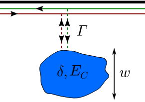
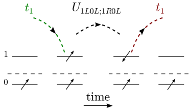
In Ref. Väyrynen et al., 2013 some of us suggested that puddles of electron liquid induced in the topological insulator by doping of a gated heterostructure may enhance backscattering. One may think of a puddle affecting the edge conductance as a quantum dot side-coupled to the helical edge by a tunnel junction, see Fig. 1. The crucial difference of the “new” quantum dot physics compared to the “conventional” one Kouwenhoven et al. (1997); Glazman and Pustilnik (2005) is that elastic scattering processes do not lead to backscattering, and therefore do not contribute to .
The confinement of charge carriers to a puddle – or a quantum dot – produces two new small energy scales: spacing between the levels of spatial quantization , and the level width associated with the dot-edge tunneling. Backscattering becomes sensitive to the position of the chemical potential with respect to the broadened single-electron levels. That makes also dependent on the gate voltage which controls the chemical potential. If it is tuned to coincide with one of the levels, then the characteristic energy scale determining the low-energy asymptote of becomes , rather than . In addition to boosting the coefficient in the power-law asymptote, the scale also defines the range of temperatures above which substantially deviates from the asymptote. In fact, the sign of the derivative can change at . If the chemical potential is tuned away from a discrete level, then the temperature dependence of strongly depends on the electron number parity in the ground state of an isolated puddle. The earlier work Väyrynen et al. (2013) concentrated exclusively on the even-parity states, where the characteristic energy separating the low- and “high”-temperature regimes is . That consideration ignored the possibility of puddles which, if isolated, would contain an odd number of electrons and thus carry spin. The spin-carrying states become ubiquitous if the puddle’s charging energy exceeds . The presence of a spin, in turn, leads to a Kondo effect and to the appearance of a new energy scale , which may be exponentially small in the parameter . The appearance of the Kondo temperature scale strongly affects the temperature dependence of since it limits the validity of the power-law asymptote to extremely low temperatures. For this reason the puddle-induced resistivity of a long edge shows remarkably weak temperature dependence. This behavior was not captured by the calculation of Ref. Väyrynen et al., 2013, which only considered puddles with an even electron number.
The goal of this paper is to develop a comprehensive theory of electron transport along the helical edge channel coupled to quantum dots formed in the “bulk” of the two-dimensional topological insulator. We concentrate on the linear-in-bias regime, and investigate for a helical edge in the presence of a single controllable dot. Some of the signature differences of the found from the two-terminal conductance across a conventional quantum dot are summarized in Fig. 2. We also aim at predicting the behavior of averaged over many random charge puddles (modeled as quantum dots) along an edge of a macroscopic sample.
 |
 |
| (a) | (b) |
As we already mentioned, the peculiarity introduced by the helical nature of the edge is the absence of elastic backscattering processes. That renders inapplicable the conventional elements of the quantum dot transport theory,Glazman and Pustilnik (2005) such as elastic tunneling in the sequential regime, elastic co-tunneling, and elastic scattering off a dot in Kondo regime, and makes us to address anew the conduction mechanisms in a broad temperature interval, from , to . Using our results we can account for the all the qualitative features seen in the experiments, namely the imperfect conductance of short samples at low temperatures and its fluctuations as function of the gate voltage König et al. (2007); Roth et al. (2009) as well as the resistive behavior of long samples. Gusev et al. (2014) We also provide detailed predictions for future experiments. Let us also note that when time reversal symmetry is broken (e.g., by applying a magnetic field) elastic backscattering caused by sources other then puddles may become significant; we therefore do not discuss this case.
The paper is organized as follows. In Section II we explain qualitatively the main results. Sections III and IV deal with the backscattering of the helical edge electrons off a single quantum dot with small or large charging energy , respectively. In Section V we estimate the puddle parameters assuming the puddles of charge originate from dopant-induced potential fluctuations. In the same section we calculate the low-temperature resistivity of a long edge due to puddles. In Section VI we discuss how our theory connects with existing experimental data. Finally, conclusions are drawn in Section VII.
Throughout this paper we use units such that .
II Qualitative discussion of the main results
In this section we give qualitative description of our main results, leaving detailed discussion to the following sections. We start with estimates of the conductance correction coming from a single dot. Being a source of inelastic scattering, it yields at low temperature; we relate the proportionality coefficient in that dependence to the parameters of the dot and establish the temperature range for this limiting behavior. The temperature dependence of outside that range turns out to be much slower, as we demonstrate next. Finally, we use the single-dot results to estimate the effect of random charge puddles on the edge resistivity of a long sample.
II.0.1 Electron backscattering off a single quantum dot.
At sufficiently low energy scales, electron scattering may be considered in the long-wavelength limit, i.e., the dot behaves as a point-like scatterer. The latter is described by an effective Hamiltonian Schmidt et al. (2012); Lezmy et al. (2012)
| (1) |
which respects the time-reversal symmetry; here is the (coarse-grained) coordinate of the scatterer. The spatial derivative in Eq. (1) accounts for the Pauli principle (). The long-wavelength limit of the Hamiltonian is applicable in some energy band . The bandwidth is determined by the structure of the impurity, which also determines the value of . Upon transformation of Eq. (1) to the momentum () representation, the spatial derivative yields a factor in the interaction amplitude. That in turn leads to an extra factor , in the scattering cross-section compared to the “standard” Fermi-liquid result,Nozières and Pines (1999) and yields , as can be checked with the help of the Fermi Golden Rule. (Here is the density of states of the edge.)
To estimate , we match the results for some scattering cross-section, evaluated in two ways: microscopically, and with the help of Eq. (1). For instance, we consider scattering of a left- and a right-mover into two left-movers, . Here is the direct product of ground states for edge and dot, , and the indices denote the propagation direction along the edge. Each state in the dot is Kramers degenerate; for each Kramers doublet we choose as a basis the states whose spin projections at the point of contact match those of the R/L edge modes at the Fermi level. We denote these dot states by R/L too. Hence, tunneling conserves the R/L index.
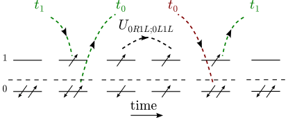
The scattering amplitude in question depends strongly on the parity of the electron number on the dot. We start with an even electron number and sketch the perturbative-in-tunneling evaluation of the amplitude. Moreover, we consider here a “toy dot” with only two orbital states. At even electron number, the state is doubly-occupied, and the state is empty (energies are measured from the Fermi level of the edge, ). A typical contribution to the scattering amplitude goes through a sequence of intermediate states (see Fig. 3): (operators create electrons in the dot). Here the first two transitions are facilitated, respectively, by tunneling of an electron into level and tunneling of an electron out of level ; the third transition is due to the matrix element of interaction within the dot , allowed by the time-reversal symmetry (for brevity we denote all the backscattering matrix elements by in the following). The contribution to the scattering amplitude reads:
| (2) | |||
Here are the matrix elements of tunneling Hamiltonian connecting the dot states with the edge, energies of the edge states are measured from the Fermi level, and is the proxy for the charging energy (coming from interaction of the additional electron on level with the two electrons on level ). The strength of momentum dispersion of the amplitude is determined by the ratio of energies in the denominators of Eq. (2) to the momentum-independent terms in the same denominator. The comparison indicates that the dispersion is negligible, as long as the energies of the involved electrons of the edge reside deep within the bandwidth , where is the dot level spacing. In the linear response regime, that sets condition on temperature, , at which one may use the effective low-energy theory.
There is a process otherwise identical to the one depicted in Fig. 3, but with the two momenta and interchanged. Adding these two and using leads to
| (3) |
where the combined amplitude is
| (4) |
(in deriving it, we accounted for the energy conservation, ). The factor in the amplitude corresponds to in Eq. (1) and nullifies the amplitude when , in agreement with the Pauli principle ( is the Fermi velocity of an electron in the edge state). In the following we take the tunneling amplitudes to be of the same order of magnitude, , and define a level width , where is the edge density of states, .
The denominator in the amplitude depends on the Fermi level position. Far away from the points of charge degeneracy, in the presence of large charging energy, or if charging is negligible. Using these estimates to simplify the amplitude (4), and then applying the Fermi Golden Rule to the Hamiltonian (3), we find
| (5) |
in the presence of large charging energy [Eq. (107), Subsection IV.2]. The result for negligible charging can be obtained from Eq. (5) by setting , see Eq. (40) in Subsection III.1. (Hereinafter in the final estimates of we use the typical value of the matrix elements for screened Coulomb interaction in the symplectic ensemble [strong spin-orbit coupling]; is the dimensionless conductance of the dot defined as the ratio of its Thouless energy to level spacing.Aleiner et al. (2002)) Note that far from the charge degeneracy points regardless of the ratio .
In the case where Fermi level is near a resonance, , the bandwidth gets reduced to and the above process (4) gives
| (6) |
The resonances with respect to and in Eq. (2) become available at temperature . When in addition , level 1 remains the only resonant level. The resonant denominators in Eq. (2) are regularized by introducing an imaginary part – this is the level width arising from tunneling between the resonant level and the edge. The correction to the conductance can be written in terms of a scattering cross section of an incoming particle of energy : . (We denote here .) The cross section is related to scattering amplitude by , where are the energies of the outgoing particles, while the energy of the second incoming particle, , is fixed by conservation of energy. The dominant contribution to comes from processes where one of the outgoing particles is in resonance, while the other is non-resonant and has energy (e.g., ; ). The amplitude for such a process is estimated from Eq. (4) to be , while its phase space volume is . We then find
| (7) |
A detailed discussion with more refined formulas for near the Coulomb blockade peak is given in Subsections IV.2.2 and IV.3, Eqs. (110)–(113). For the limit of weak charging interaction, see Eqs. (37)–(39).
We assumed above that the ground state of an isolated dot has an even number of electrons. While this is always the case for small charging energy, a strong charging interaction makes it possible to tune gate voltage so that the dot ground state has an odd number of electrons. Such a ground state is doubly degenerate and can be thought of as two states of a spin-1/2 particle. One can then derive an effective Hamiltonian
| (8) |
valid in the energy band and describing exchange interaction between the dot spin and the edge spin density at the point contact. The exchange coupling can be split into isotropic and anisotropic parts, . The isotropic part may be related to the properties of the single-occupied state, similar to how it is done for the Anderson impurity problem.Anderson (1966) Notably, for a point-contact the spin-orbit interaction does not lead to exchange anisotropy in the single-level approximation. 111this limitation is lifted if the tunneling region is extended, see Appendix A To find the anisotropic part (which reflects the presence of spin-orbit interaction), one has to account for the multi-level structure of the dot and the intra-dot interaction between the electrons.
Let us first consider only the isotropic part . Connecting to our microscopic Hamiltonian, can be writtenAnderson (1966) as the amplitude of an edge electron tunneling into and out of the singly-occupied level ,
| (9) |
Here is the cost in charging energy to empty level . The isotropic part leads to the familiar definition of Kondo temperature . At one may generalize the “poor man’s scaling” ideas Anderson (1970) to find . The result is a weak (logarithmic) temperature dependence in the temperature interval . The physics of Kondo effect in a helical edge is somewhat different from the conventional one in quantum dots,Glazman and Pustilnik (2005) and we sketch it next.
Unlike in the conventional quantum dot case,Glazman and Pustilnik (2005) the isotropic part of does not contribute to backscattering. It can be shown with the following argument. The dc backscattering current can be expressed in terms of time derivative of the numbers of right- and left-movers (of the edge) in a steady state, . None of the edge (or dot) spin-projections are in general conserved, but we can nevertheless define a hypothetical spin by using the orthogonal Kramers states. We take the -projection of this edge net “spin” to be proportional to the above difference, . If the exchange interaction between the dot and helical edge would be isotropic, then -component of the total spin is conserved, ; as the result, , where is the -component of the dot spin. The latter one is bounded, ; hence, in steady state and Tanaka et al. (2011) . We note that in a steady state at bias . Finding may be reduced to a problem of equilibrium statistical mechanics. Using the general principle Landau and Lifshitz (1980) of constructing Gibbs distribution , we form a linear combination of the Hamiltonian and integral of motion ,
| (10) |
The factor ensures that the chemical potentials of the left and right movers differ by due to the applied bias. 222using the equilibrium distribution is compatible with having different chemical potentials of the two fermion species due to the presence of the integral of motion We may neglect in Eq. (10) as long as and . After that, finding average spin polarizations becomes trivial, at ; the dot spin polarization is in equilibrium with the itinerant electron polarization at the Fermi energy. (Polarization here is defined in the Kramers-pair sense.) Inclusion of a small anisotropic part into the exchange coupling breaks the integral of motion, and, in analogy with the Bloch equations Bloch (1946) [see Eq. (86)] we expect . Here is the analogue of the Korringa relaxation rate Korringa (1950) which in our case accounts only for the interaction violating the conservation; and are some dimensionless constants depending on the specific form of the tensor . At the same time, small should leave the steady-state values and close to the equilibrium values at . As the result, we find (see also Ref. Tanaka et al., 2011) [Eq. (98)]
| (11) |
The logarithmic correction in the brackets is the harbinger of the Kondo effect, which develops at .
The anisotropic contribution to the exchange is generated by processes that involve, in addition to electron tunneling into and out of the dot, an interaction-driven transition between the levels within the dot. An example of such a process has an amplitude (see Fig. 4)
| (12) |
where level 1 is empty in the ground state. The energy can be directly controlled with gate voltage and ranges from to when moving from the middle of the valley to the charge degeneracy point (Note however that the exchange Hamiltonian (8) is not valid for , see Subsection IV.1.3.) For brevity of notation, hereinafter we absorb in , so that . Later on, in Subsection IV.1.1, we will be considering a generic large dot with many levels – this leads to summation over empty levels, yielding an extra factor in the amplitude . To be consistent with the later general results, we introduce this factor into the amplitude. The resulting estimate for the anisotropic part of the (bare) exchange is . Using this estimate in Eq. (11) leads to
| (13) |
[We assumed here for simplicity that in Eq. (9).] This result is perturbative in , thus requiring . As one lowers the temperature , the exchange couplings get renormalized. Summing the leading log-series leads to a suppression Anderson (1970) of by a logarithmic factor [Eq. (103c)],
| (14) |
Below the Kondo temperature we can use the low-energy Hamiltonian (1) to get . By matching this with Eq. (14) in the limit we can read off . The new low-energy bandwidth is ; for within it, we get [Eq. (103c)]
| (15) |
Far from the points of charge degeneracy, is smallest, and consequently is exponentially small. That makes the temperature dependence of weak, see Eqs. (13) and (14), in a broad temperature interval .
Close to the charge degeneracy points, , the exchange constants substantially increase leading to in Eqs. (13), (15), which match then the estimates of the peak values of given in Eqs. (7), (6).
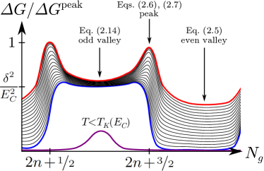
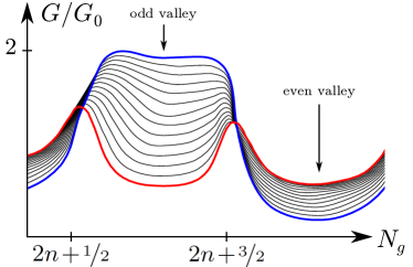
The key features of the temperature and gate voltage dependence of are illustrated in Fig. 2a. (For a contrast, we present in Fig. 2b the conductance vs. gate voltage and -dependence for a “conventional” quantum dot device.van der Wiel et al. (2000)) At low temperatures , the conductance correction displays strong dependence on gate voltage, seen as peaks [Eqs. (6), (7)] and valleys [Eqs. (5), (14), (15)]. Furthermore, the valleys with an odd number of electrons differ significantly from those with an even number [cf. Eq. (5) vs. Eq. (14)].
Upon increasing temperature, the difference between peaks and valleys is seen to decrease, while the average increases as a function of temperature. Also the distinction between odd and even valleys disappears once temperature is increased, , since spin-carrying particle-hole pairs become thermally populated regardless of dot particle number parity.
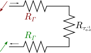
Upon further increase of temperature, , also the particle number of the dot is allowed to fluctuate, washing away peaks and valleys, making weakly dependent on gate voltage. At these high temperatures the virtual processes described above [Eqs. (5)–(15)] give way to sequential tunneling. The conductance correction can then be thought of as the conductance of a quantum dot coupled to spin-polarized “leads” (the left- and right-moving edge channels), see Subsection III.3. Then corresponds to three resistors in series: two identical resistors corresponding to weak tunneling between the edge (or “leads”) and the dot and a third one corresponding to the necessary spin-flip process inside the dot, see Fig. 5. The latter is characterized by the intra-dot scattering rate , and exceeds the rate of tunneling at temperatures . Above this temperature nearly every electron that finds its way into the dot loses memory of its origin and has equal probabilities to tunnel back as a left or a right mover. The bottleneck for backscattering then lies in tunneling in and out of the dot. Then saturates to the constant value [Eq. (68)] given by tunneling rate times the dot density of states,
| (16) |
Taking the limit , corresponding to a dot lying on the edge, we find in agreement with the theoretical model used in Ref. Roth et al., 2009. There the authors showed that a completely phase-randomizing dot on the edge has the same effect on edge conductance as an additional lead.

The overall temperature-dependence of of a single Coulomb blockaded quantum dot is summarized in Fig. 6.
II.0.2 Correction to the conductance due to many Coulomb blockaded puddles
In this section we show how many quantum dots (or charge puddles) affect the resistivity of a long edge. It is assumed that the presence of many puddles does not lead to appreciable bulk conductivity at low temperatures. For doping-induced puddles this requires low enough dopant density; the crossover value of the dopant density is determined by the properties of the heterostructure Gergel’ and Suris (1978) and is given in Eq. (126) in Subsection V.1.
The backscattering of edge electrons off a quantum dot is inelastic and therefore incoherent. It means that the conductance correction from several puddles is additive, and the self-averaging resistivity of a long edge is obtained by independently summing over single-puddle contributions, , see the derivation of Eq. (133). Here is the number of puddles per unit area in the bulk, is the penetration depth of the electron wave function into the bulk (determined by bulk band gap and the Dirac velocity in HgTe), and is the single-puddle conductance correction averaged over the puddle parameters and the number of particles in it. This last average can be done by keeping the dot levels fixed and averaging over the chemical potential, or, equivalently, the gate voltage.
We consider the most interesting case of low temperatures, , where bulk conductivity can be safely ignored. In the presence of charging , the average of over number of particles is dominated by odd occupations (see Fig. 2a). For averaging we need to take into account properly the gate voltage dependence of the Kondo temperature and . The valley is symmetric, so it suffices to consider the gate voltage interval from the bottom of the valley to the peak separating dot charge states 1 and 2, . We also need to sum over different distances between the edge and the dot. This sum can be converted into an integral over the edge-dot tunneling rate , which decays exponentially with the distance between the dot and the edge, . The upper limit for is the level spacing , as follows from our assumption of narrow levels. 333The lower limit is non-zero for a finite width sample where . Here we however assume a wide enough sample, so that the lower limit can be taken smaller than any other scale As was already mentioned, the average is dominated by the odd valleys and more specifically by those gate voltages where is valid. In this interval the logarithmic corrections to the bare value of are small and we can use the first term in Eq. (13). The average conductance is then
| (17) |
Inserting [see Eq. (9)] in the Kondo temperature allows us to write the step function as a condition on level width: . If this condition is stricter than , then it is the step function rather than upper limit that determines the domain of integration over . We will confine our considerations to that limit, realized at low temperatures, . We then get from Eq. (17) the average at low temperatures,
| (18) |
Application of standard methods of disordered semiconductors theory Gergel’ and Suris (1978); Shklovskii and Efros (1984) to a doped heterostructure allows one to conclude that typically and at weak doping. This condition is sufficient to yield a substantial fraction of puddles carrying an odd charge. Equation (18) then yields a long-edge resistivity with a weak temperature dependence [Eq. (136)]
| (19) |
This equation is one of the main results of this paper, and concludes the qualitative part. We would like to point out that the above result differs from that given in Ref. Väyrynen et al., 2013 (), where the odd occupations were not accounted for. We now turn to detailed calculations, starting with the evaluation of in the weak-interaction limit (i.e., in the absence of Coulomb blockade).
III Electron backscattering in the absence of charging effects
We consider a time-reversal (TR) symmetric Hamiltonian of a helical edge coupled to a quantum dot. The coupling is assumed to be via a point contact with tunneling matrix elements ; generalization to a line contact is given in Appendix A. For a TR-symmetric point contact the matrix elements can be chosen to be real with a rotation of the spin quantization axis of the dot (Appendix A). More specifically, the rotation aligns the dot spin quantization axis at the point contact to be parallel with that of the edge electrons at the Fermi level.
The finite-size quantum dot is assumed to be in the metallic regime (dimensionless conductance ) with a set of discrete random energy levels whose distribution is described by random matrix theory (RMT) (with mean level-spacing ). The free part of the Hamiltonian then reads
| (20) | ||||
where the point contact is at on the edge, and labels the Kramers pairs in the dot and the edge (left- and right-movers). Note that the free Hamiltonian is diagonal in this label. The discrete levels of the quantum dot are measured from the Fermi energy. The tunneling between the edge and the dot results in a finite lifetime to the eigenstates of the dot. We denote the decay rate, or level width, of level by . Interactions in the dot are described by the Hamiltonian
| (21) |
By TR symmetry, the interaction matrix element satisfies , denoting for Kramers indices. Note that the TR symmetry does not prevent from having matrix elements that do not conserve the total spin of the two electrons. The typical value of the squared matrix element is given in Appendix B. In this section we consider weak charging effects, i.e., the limit where all non-zero matrix elements of interaction are small. The perturbative treatment of the entire interaction Eq. (21) is possible when the matrix elements are small compared to .
In absence of , we define the free retarded dot-dot Green function as
| (22) |
It satisfies the Dyson equation
| (23) |
where is the dot Green function in absence of tunneling, and is the self-energy. Here is the edge state dispersion relation. From TR symmetry, , it follows that the self-energy is independent of . The imaginary part of the self-energy broadens the dot levels,
| (24) |
where is the single particle density of states, which is assumed to be energy-independent. (By TR-symmetry, the density of states is the same for both Kramers pairs, and we can leave out the index .) As a matrix in the levels space, the solution to Dyson equation is then
| (25) |
where .
We are interested in how the coupling of the helical edge to the quantum dot (and interaction within) affects the conductance of the edge. To this end, we need to consider scattering processes between exact left- and right-propagating eigenstates of the single-particle Hamiltonian. In the Born approximation the amplitude for these processes is . The corresponding scattering cross section can be written as a sum over dot-eigenstates,
| (26) |
The correction to the edge conductance can be expressed in terms of the cross section. Inelastic backscattering due to reduces the steady-state current from its ideal value by ,
| (27) |
Here is the source-drain voltage, counts the net number of backscattered particles, is the Fermi function shifted by . A two-electron process allows backscattering of one or two electrons. We will denote these contributions as :
| (28) |
When the tunneling is weak and individual levels are well-defined, , the dot-dot Green function can be calculated approximately by expanding Eq. (25). The leading order approximation in for diagonal and off-diagonal parts of is
| (29) | ||||
| (30) |
These equations are valid for all real frequencies .
III.1 The correction to the conductance at low temperature,
Let us first consider low temperatures, . In linear response, the energies of the external states in Eq. (26) are restricted by the Fermi functions and energy conservation to be within of the Fermi energy. Therefore the backscattering current depends strongly on the position of the Fermi level which is controlled by an external gate in experiments. This leads to peaks and valleys in the conductance as a function of Fermi level position. Peaks correspond to a level close to the Fermi level and their widths are determined by the temperature or the level widths, . Here the level energy is measured from the Fermi energy. Note that since charging effects are neglected in this section, the ground state of the quantum dot is non-degenerate and always has zero total spin.
Consider first the valley conductance correction . In this case the energies of external states in Eq. (26) are far from the resonances. Using the Green functions of Eqs. (29) and (30) the cross section for a process is to leading order
| (31) | ||||
The factor results from antisymmetrizing over the indices , in the Green functions, by using the fermionic property of the interaction matrix elements. For backscattering of one particle ( above), which can be done in four ways, one gets a conductance correction
| (32) |
For backscattering of two particles ( above) we can also antisymmetrize over the indices , resulting in an extra factor giving 2 extra powers of temperature in the conductance. We get
| (33) |
The two-particle backscattering Eq. (33) is thus suppressed by a factor compared to single-particle contribution, Eq. (32), at low temperatures.
Consider now the peak conductance correction . Let one of the levels, , be near the Fermi energy but far from other levels, . The cross section for is dominated by processes that involve the level ,
| (34) | ||||
For one-particle backscattering we can choose above to take full advantage of the resonant level. For two-particle backscattering we can at most set , leading to in Eq. (28), as we will see below.
In the limit of relatively high temperature, , the resonance condition allows us to replace (for all in the case of one and in the case of two backscattered particles) in the Fermi functions of Eq. (27). The Lorentzians are then easily integrated-over and at the peak () is
| (35) |
for one-particle backscattering, and
| (36) |
for two-particle backscattering.
In the opposite limit, , the denominators of the cross section depend weakly on the energies . We find for backscattering of one particle,
| (37) |
and for backscattering of two particles,
| (38) |
Comparing the one- and two-particle contributions in Eq. (28), we see that . At low temperatures the effects of two-particle backscattering are negligible compared to those coming from one-particle backscattering.
The above results are valid for a single quantum dot and the conductance correction is dominated by the one-particle backscattering processes. Averaging over energy levels (see Appendix B), and replacing level widths by their typical values, we obtain from Eqs. (35) and (37) the interpolation
| (39) |
Similarly from Eq. (32) we find
| (40) |
where and are, respectively, the mean level spacing and level width. We used for the average interaction matrix elements, assuming screened Coulomb interaction and strong spin-orbit interaction, Note (8) see Appendix B.1. Here is the dimensionless conductance of the dot, being its Thouless energy. The factors and are coming from level statistics, see Appendix B.2. The average of the above results, Eqs. (39) and (40), over the Fermi level position, , is dominated by the peaks, and we get
| (41) |
III.2 Crossover to higher temperatures,
In the above we looked at low temperatures, . Next, we will study higher temperatures, where direct tunneling gives the dominant contribution to backscattering, and peaks and valleys seen in the previous subsection are washed out. We will see below that the crossover happens at . This is somewhat similar to conventional quantum dot transport where the low temperature transport is dictated by virtual elastic and inelastic processes (so-called cotunneling), while thermally activated direct tunneling takes over at higher temperatures.Glazman and Pustilnik (2005) In the case of a helical edge coupled to a quantum dot the picture remains qualitatively the same, except that elastic cotunneling is absent (see previous subsection). We will now investigate what is the conductance correction due to direct tunneling.
Direct tunneling amounts to using only diagonal Green functions, Eq. (29) in the backscattering cross section, Eq. (26). One gets a correction to the linear conductance
| (42) |
where . There are two distinct types of contributions to . The first one involves transitions within a pair of levels, , and takes the full advantage of the resonant tunneling processes. The other one involves more levels, , and gains importance as the temperature increases due to the broadening of the available phase space. At temperatures much lower than the average level spacing, , it is enough to consider only the two levels nearest to Fermi energy. Then Eq. (42) reduces to
| (43) |
Comparison with Eq. (37) shows that the crossover from cotunneling to direct-tunneling occurs at .
At higher temperatures, (but still so that RMT-description is valid), many levels contribute in Eq. (42). Using average values for dot parameters and screened Coulomb interaction, Eq. (161), we find
| (44) |
The first term in Eq. (44) comes from processes involving only a pair of levels in Eq. (42), while the second term involves four levels. It is instructive to interpret the first term: To estimate the backscattering current , we note that the levels participating in the backscattering processes are located within an energy strip around the Fermi level. The number of levels admitting, say, two right-movers is . The rate of scattering for the two-level process in the dot is , with being the density of states for a tunnel-broadened level. Finally, the imbalance between the numbers of right- and left-movers is determined by the applied bias voltage . Collecting all of the above factors, we find
| (45) |
yielding, up to a numerical constant the first (two-level) term of Eq. (44). The multi-level backscattering (the last term) starts to dominate over the 2-level backscattering at temperatures . Its form is closely related to the electron relaxation rate in the dot,Sivan et al. (1994) , as we discuss in Subsection III.3.
Equations (39), (41), (43), (44) contain seemingly divergent contributions in the limit . These terms describe resonant tunneling from the helical edge into the dot, and the limiting factor to backscattering is the intra-dot interaction : Electrons tunnel frequently into the quantum dot but they also leave fast and only those few who stayed long enough get backscattered by . In the limit tunneling becomes weaker and all tunneled electrons have time to scatter multiple times in the dot. In this limit perturbation theory in breaks down (as indicated by the divergences). Indeed, the above results were obtained in the Born approximation, valid when the backscattering matrix elements (those corresponding to processes with ) are small with respect to the level widths and form the bottleneck for backscattering. In the opposite limit, , the bottleneck shifts to the tunneling in and out of the dot, and the backscattering rate saturates at a value independent of . The full crossover behavior is complicated in general; for a toy model with only the two-electron backscattering matrix element present, Eq. (43) is generalized by the replacement (see Appendix C):
| (46) |
Similarly, the validity of the first term in Eq. (44) requires ; in the opposite limit of smaller this term would be replaced by a term .
The Born approximation in the interaction may fail even if as one raises the temperature. At high temperatures the levels broaden due to the large phase space available for electron-electron scattering. For screened Coulomb interaction, the level broadening due to the electron-electron scattering, , exceeds the many-particle level spacing, , at . In this “high-temperature” regime one may replace the dot spectrum by a continuum.Altshuler et al. (1997) Such a replacement allows us to develop a kinetic equation approach and evaluate in the regimes beyond the one described by Eq. (44).
III.3 The kinetic equation
In the kinetic equation approach it is useful to think of as the conductance of a quantum dot tunnel-coupled to two (left and right) fictitious spin-polarized leads, see Fig. 5. The leads model the helical edge, if we assume that the left and right leads are reservoirs of respectively - and -particles. The Kramers labels are conserved in tunneling into and out of the dot. For a non-zero steady-state current through the dot to exist, there needs to be inelastic intra-dot spin-relaxation which converts - and -particles into each other.
Let denote the distribution function inside the dot ( labels the degenerate Kramers pairs, is the single-particle level) and for the left and right leads. We refer to the index as just “spin” of the state. We write as a sum of the equilibrium part (the Fermi distribution) and a small deviation, . Without interaction in the dot we have the linear rate equation
| (47) |
where , with the edge density of states, which is assumed to be independent of energy. In this case in steady state it is easy to see that the current into the dot vanishes. To facilitate comparison with conventional quantum dot tunneling results, we will keep the index in the tunneling rates, i.e., left and right leads have in general different tunneling rates. In the physical system these rates are equal as dictated by TR symmetry (see Appendix A).
The dot relaxation can be treated by the Fermi golden rule. The inelastic contribution to the rate equation is
| (48) |
it vanishes in equilibrium . The above equation becomes meaningful when averaged over realizations of disorder, i.e., dot levels.Sivan et al. (1994) We define the average distribution function as where is the average density of levels and denotes averaging over disorder. For convenience, we will also denote the equilibrium distribution by , where is a Fermi function. Assuming small deviation from equilibrium distribution at small bias, we can linearize the collision term Eq. (48) to get
| (49) |
In the above equation we have split the averages of products in Eq. (48) into products of averages, which is justified,Altshuler et al. (1997) if the level broadening exceeds the many-particle level spacing, . This condition leads to the constraint . Furthermore, we ignored terms with in Eq. (48). These formally diverging terms are regularized by the level broadening. The broadening is provided by tunneling (at rate ) and by scattering to other levels in the dot. The scattering processes with are responsible for the first term in Eq. (44). Ignoring them limits the applicability of the kinetic equation (derived below) to temperatures , see the discussion following Eq. (44).
The two terms on the right-hand side of Eq. (49) are “out” and “in” contributions. In the “out” part, gives the inverse lifetime of the state with energy ; it is independent of spin because of TR symmetry. For the “in” term TR symmetry dictates that , so that this kernel consists of only two independent elements, , which characterize forward- and backscattering respectively. The explicit expressions for and obtained from Eq. (48) are (here is the equilibrium Fermi function of the dot and energies are measured from the Fermi level):
| (50) |
and
| (51) |
Here
| (52) |
has the symmetries
| (53) |
and TR symmetry .
For the special case of screened Coulomb interaction [Eq. (161)] we have
| (54) |
and the scattering rate becomes Sivan et al. (1994)
| (55) |
The number of particles and total energy are conserved, as is manifested in the following relations between the kernel and lifetime ,
| (56) | ||||
| (57) |
In addition,
| (58) |
where . Hence the collision term, Eq. (49), vanishes in equilibrium, as it should. Note that , and () is the rate of backscattering (forwardscattering).
Including the collision term we can write the full disorder-averaged rate equation
| (59) |
where is generally energy-dependent, and the last term is the intra-dot relaxation,
| (60) | ||||
In the steady state we have in Eq. (59), hence
| (61) | |||
The current into the dot is
| (62) |
It follows from particle number conservation, Eq. (56), that . It is useful to write the current in the symmetric way
| (63) | |||
Inserting the steady state equations (61) in the current, we get
| (64) |
We see that the current is determined by the rate of backscattering and the deviation of the dot distribution function from that in equilibrium. Next, we will solve the steady-state equation (61) for the difference in the case of equal tunneling rates, , and strong spin-orbit scattering, , corresponding to symplectic RMT ensemble assumed in the previous subsection.
With strong spin-orbit coupling the kernels for backward and forward scattering are equal, . As the tunneling rates are identical for the two spin species, subtracting Eq. (61) with from that with leads to
| (65) |
The conductance is
| (66) |
where . The main contribution to the integral comes from . For screened Coulomb interaction, Eq. (55), the conductance is
| (67) |
where is a dimensionless integral,
The low- and high-temperature limits of Eq. (67) are
| (68) |
Now we are ready to discuss the temperature dependence of in a broader interval, covered by Eqs. (44) and (68). As we already mentioned after Eq. (44), the crossover from the two-level contribution to the four-level dominated one in backscattering occurs at . This latter contribution crosses over from to -independent value at , see Eq. (68) and Fig. 7. At these two crossovers follow one after another, as . At , the two characteristic temperatures change their order, , see Fig. 7. Under this condition, the broadening of levels induced by interaction may affect the two-level contributions described by the first term of Eq. (44). The behavior of can be assessed by the proper modification of that term’s interpretation given after Eq. (44). Level broadening diminishes the density of states entering in the transition rate from to . As the result, we find an interpolation
| (69) |
which at matches, up to numerical factors, the first term in Eq. (44), and at the high-temperature asymptote of Eq. (68).

In conclusion, above we investigated the temperature dependence of the conductance correction in the absence of charging effects. It has a universal asymptote, , at low temperatures, and saturates to a constant value at fairly high temperatures, . We also saw that varies substantially in between. There is no intermediate, parametrically large temperature interval where can be fairly approximated by a constant. This is in contrast with a Coulomb blockaded quantum dot where, due to Kondo effect, there is a broad range of temperatures characterized by a weak -dependence, as we will see in the next section.
IV Coulomb blockade of the electron backscattering
In the previous section we considered the effect of weak interaction in the quantum dot. It means that even the largest (and universal Aleiner et al. (2002)) part of interaction (21), i.e., charging energy, , is small compared to level spacing . Whether this is the case in a real-world experiment depends on the parameters in the measurement setup (see Subsection V.1 for more details). Generally, the capacitance of a quantum dot of linear size and distance from a gate can be approximated as , where is the dielectric constant. Similarly, the level spacing depends on the size of the dot, but also on the bulk band structure. We consider here a massive Dirac spectrum appropriate for HgTe near the band gap. Bernevig et al. (2006) We denote the effective mass by , with being the band gap and the Dirac velocity. We find that the average level spacing is , interpolated here between the linear () and quadratic () parts of spectrum. (Here is the Fermi momentum.) Since , we get for the relative strength of charging energy,
| (70) |
Here we introduced the effective Bohr radius , where is the effective fine-structure constant. From Eq. (70) we see that if the puddles are large and well separated from the gate electrode, , the charging interaction becomes important.444 For example, for HgTe with , , and one finds Gusev et al. (2014) . We therefore think that it is relevant to discuss the case where the condition of Section III is not met (see also Subsection V.1).
In this section we turn to study strong charging effects, , corresponding to a large universal part of the interaction compared to the level spacing. Replacing these large diagonal matrix elements by their random-matrix averages leads to the so-called universal Hamiltonian of the isolated dot,Aleiner et al. (2002)
| (71) |
where is the charging energy of the dot, being its total capacitance. The tunable parameter is controlled by the gate voltage applied between the metal gate and the quantum well, where is the dot-gate capacitance. In its ground state the dot is populated by the nearest-integer-to- number of electrons . The charging energy required to add an electron into the dot is , while the cost of removing one is .
Integer values of correspond to Coulomb blockade valley centers where the energy costs of adding or removing an electron are equal, . In the even valleys ( even) the correction to the helical edge conductance scales as at . In the odd valleys ( odd) exhibits a very different behavior because of a degenerate ground state due to the electron spin. We will see that the degeneracy gives rise to an emergent scale (the Kondo temperature, ), and that the conductance correction becomes logarithmic in temperature at . At half-integer values of , the dot states with and electrons are approximately degenerate. This gives rise to a large conductance correction (a peak in vs. dependence), which has only a weak dependence on temperature at .
Let us denote by the Hamiltonian of the decoupled helical edge and quantum dot, . We treat the non-universal part of the interaction (denoted by in this section) and the tunneling between the edge and the dot as perturbations,
| (72) | |||
At low temperatures, , and away from the peaks, the backscattering current is dominated by high-order tunneling processes. Generally the rate of transition from an initial state to a final state is
| (73) |
Here is the thermal probability of the initial state . It factorizes to parts corresponding to the dot, and the left and right Kramers states of the edge, . The -matrix is suited for high-order perturbation theory, and satisfies
| (74) |
where we denote . The solution can be written as
| (75) |
In the following sections we use this formalism to calculate the correction to helical edge conductance, , due to scattering off a Coulomb-blockaded quantum dot. In Subsection IV.1 we describe the conductance correction in the odd valley, and we show that due to a degeneracy of the dot ground state, an effective exchange-type interaction can be derived from the appropriate low-energy -matrix. The even valley of the Coulomb blockade is discussed in Subsection IV.2. There the ground state of the isolated dot has an even number of particles and is thus unique. We use a low-energy -matrix that accounts for the most important virtual processes. In Subsection IV.3 we find the conductance correction near the charge degeneracy point (peak) between an even and an odd valley. The limit of high temperatures is discussed in Subsection IV.4. In the same section we look at even higher temperatures, , and make connection to Subsection III.3. Finally, in Subsection IV.5 we calculate the average of the conductance correction over the gate voltage at low temperatures .
IV.1 Odd Coulomb-blockade valleys
In this section we discuss the low-temperature, , backscattering in the odd valleys where the gate voltage is tuned so that the number of particles in the dot, , is odd. The ground state of the isolated dot is then doubly degenerate, corresponding to the two Kramers states of the odd electron. These two states can be viewed as those of a spin-1/2 particle, and a weak tunneling between the edge and the dot results in an exchange coupling between the itinerant electrons and this spin. The tensor of exchange coupling constants is constructed in Subsection IV.1.1, by deriving perturbatively the low-energy -matrix. Because of virtual processes violating spin conservation in the dot, the exchange coupling tensor generally cannot be diagonalized by a rotation of the dot effective spin. We show in Subsection IV.1.4 that this anisotropic exchange coupling results in backscattering of electrons. To assess the correction to the conductance, we first use a Bloch equation to calculate the steady-state expectation value of the dot spin in Subsection IV.1.2. In Subsection IV.1.3 we show that our perturbative approach is valid at temperatures much larger than an emergent temperature scale, the Kondo temperature . Finally, as already mentioned, the correction to the conductance introduced by a spin-carrying dot is evaluated in Subsection IV.1.4. In the same section we also show how to extend our results to near and below the Kondo temperature, and , respectively.
IV.1.1 Derivation of the effective Hamiltonian.
In this section we derive the low-energy Hamiltonian of the tunnel-coupled interacting edge-dot system. We start with the full Hamiltonian , where is the Hamiltonian of the decoupled edge and dot [charging energy included, Eq. (71)], is the non-universal part of the intra-dot interaction, and is the tunnel coupling between the edge and the dot. The weak perturbations and can create high-energy excitations above the ground state of . We perturbatively project out these high-energy states (of energies ), leaving us with a new Hamiltonian valid in a strip of energies around the edge Fermi level. At low temperatures this new Hamiltonian accurately describes the exchange interaction between the edge and the dot. To classify these high-energy states, we start by discussing the ground state and excitation spectrum of .
By tuning the gate voltage so that is close to an odd integer , the ground state of the dot has a single electron on the highest occupied level (note that , as the energy is measured from the Fermi level). This ground state is doubly degenerate because of the Kramers degeneracy of that level, and we denote the two ground states by and . The perturbations and create excitations from the ground state of describing the decoupled edge-dot system. The respective excitations correspond to removal/addition of an electron from/into the dot, and to creation of an electron-hole pair in the dot. The energies of these excitations are of order and , respectively, which prompts us to take . Then at energies within the band such excitations only occur in virtual processes, allowing a simplification of the -matrix (75).
The low-energy -matrix can be derived perturbatively from the Dyson equation (74) by separating the high- and low-energy states. Anderson (1970) For this we introduce projectors , and . The first one, , projects the dot to its ground state with spin . The three other projectors project to the high-energy subspace: projects to states with at least one particle-hole excitation above the dot ground state, but no change in dot particle number. Projectors project to states where the dot has an excess (+1) or deficit (-1) of one particle (and possibly particle-hole excitations). To lowest order in tunneling we do not need to consider virtual dot states with more than one particle added or removed. Projecting Eq. (74) into the low-energy subspace and casting the resulting equation in the form of Eq. (74) with a modified perturbation, , and considering only the first order in and second order in tunneling , we get
| (76) |
Here is the energy of the dot in its ground state, and we denote where is one of the projectors , , . We also used the fact that at low temperatures we can neglect in the denominators the energies of the edge excitations in comparison with those of the virtual states. From TR symmetry it follows that the first term gives just a constant shift in energy, , and we will ignore it from now on. The second term is independent of the interaction , and gives the known isotropic anti-ferromagnetic exchange interaction, see Eq. (80). The remaining terms in Eq. (76) bring in the exchange anisotropy.
Considering only the exchange terms, we can write the effective Hamiltonian as
| (77) |
where is the spin-1/2 operator of the dot, and is the edge spin density at the point contact,
| (78) |
We find that the exchange tensor obtained from Eq. (76) can be written as , where is a rotation matrix acting on the dot spin, and is a lower triangular matrix (in the basis). In the basis of rotated dot spin, , we get
| (79) |
The full expressions for components and in terms of dot parameters are given in Table 1 of Appendix E. The leading contribution to is the familiar exchange coupling of the Anderson Hamiltonian,Anderson (1966)
| (80) |
where denotes higher order corrections that are smaller than the main term by a factor [see Eq. (179) in Appendix E]. As an example of the anisotropic terms we give,
| (81) |
Generally the isotropy breaking terms are smaller by a factor compared to . We will see below that the isotropic part of will not contribute to backscattering.
IV.1.2 The Bloch equation and its steady-state solutions.
Passing a current along a helical edge leads to spin polarization of a quantum dot coupled to the edge by the exchange interaction. The spin polarization , in turn, affects the backscattering. In this section, we derive the Bloch equations Bloch (1946) for . We use the standard scheme for the derivation. First we use the Heisenberg equation of motion to relate to the higher-order correlators (here is the operator of spin density of the helical edge at the point of contact). Second, we express the correlators in terms and perturbatively, to the first order in . That procedure yields the spin relaxation rates to the second (lowest non-vanishing) order of perturbation theory in . To illustrate, using Eqs. (77) and (79) we get, for example,
| (82) |
where has zero average, and the first term in Eq. (82) comes from , where is the edge density of states per spin, . Here we have chosen the spin quantization axis of the edge electrons at the Fermi level to be along . Expressions similar to Eq. (82) hold for derivatives of and . Next, we use lowest-order perturbation theory in to evaluate the right-hand side in Eq. (82). For any operator we have
| (83) |
Using the above formula we get, for example, that
| (84) |
where
| (85) |
The last equality is the expansion of for small bias , and is the bandwidth. The logarithmic term here is a variety of a Kondo correction. Hewson (1997) We will ignore these corrections in this section. The justification for this is given in the next section. In Subsection IV.1.4 we show how the Kondo effect is accounted for.
Combining Eqs. (82) and (84), and similar equations for other components of and pair averages, we find Bloch equation in the form
| (86) |
with
| (87) |
where is the unit vector along the spin quantization axis of the edge electrons at the Fermi level,
| (88) | ||||
and,
| (89) |
Here and are given to linear order in both the bias voltage and the deviation from isotropic exchange.
The steady-state expectation value of is obtained by setting the left-hand-side of Eq. (86) to zero. For small bias , and thus as well, hence to linear order in the bias voltage the cross-product term in Eq. (86) can be neglected and we can approximate the steady-state value of the spin as . Expanding to first order around the isotropic , we have
| (90) |
The first term here is independent of . This is a consequence of equilibrium being established between the dot and the edge with unequal populations of left and right movers at , see Eq. (10) and the related discussion. The two other terms in Eq. (90) have kinetic origin associated with the anisotropic part of .
IV.1.3 Validity of perturbation theory, the Kondo temperature
The perturbatively evaluated “bare” exchange constant, Eq. (80), is small, . In the conventional magnetic impurity problem, the renormalized exchange constant increases with the energy (or temperature) being lowered below , due to the Kondo effect. Hewson (1997) This is also the case here, as can be seen from the first two corrections in powers of to . This average can be evaluated by thermodynamic perturbation theory applied to the Gibbs distribution Eq. (10). Similar to the conventional Kondo problem, the corrections to in Eq. (90) are small when and Hewson (1997)
| (91) |
This equation defines the Kondo temperature ,
| (92) |
which depends on the gate voltage. To lowest order in the non-universal part of intra-dot interaction we have [see Eq. (80)]
| (93) |
( is the width of the level .) The Kondo temperature can be written as (we absorb into )
| (94) |
We always have which gives a lower bound,
| (95) |
for the Kondo temperature, reached in the middle of the Coulomb blockade valley. As one moves closer to a peak so that , the Kondo temperature becomes , and has its maximum at .
Our perturbation theory in is thus valid when , where both and depend on gate voltage (through ). Near the peak , and the assumption fails, as can also be seen from Eq. (93). Likewise, the required condition on temperature cannot be satisfied at any gate voltage if . At such low temperatures, , the logarithmic corrections to become large. In this strong coupling regime, one can write a phenomenological Fermi liquid model as we demonstrate in the next subsection.Nozieres (1974) The correction to the conductance in both the perturbative and non-perturbative regimes is discussed there.
IV.1.4 The correction to the conductance
The coupling of the edge electrons to the spin of the dot modifies the ideal conductance of the edge. The correction to the conductance, is calculated, e.g., from the change in the number of left moving electrons on the edge in the steady state. Denoting , the backscattering current is . It is convenient to add to the current a term which has vanishing time-average since it is the time-derivative of a bounded operator. Upon this addition, the current takes the form
| (96) |
The advantage of the modification is in the fact that the operator in the square brackets is an integral of motion if the exchange coupling is isotropic; it’s time variation is associated only with :
| (97) |
We can use Eq. (84) and its companions to express the averages in in terms of . Inserting the steady-state solution (90) we get a correction to the conductance
| (98) |
Here the components are given in Table 1 of Appendix E. They depend on the dot parameters as well as on the gate voltage, and generally grow in magnitude towards the peaks. We can extend the above formula to lower temperatures, , by using the standard renormalization group technique, see Appendix F.
As one moves towards low temperatures, the logarithmic corrections to become non-negligible, see Subsection IV.1.3. The anisotropic components of (which enter ) are irrelevant perturbations, as shown by the renormalization group analysis carried out in Appendix F. Accordingly decreases with :
| (99) | |||
Here is the “bare” exchange coupling and the renormalization (“dressing”) is given by the logarithmic factor, see Appendix F. This factor is of order unity at high temperatures, , but becomes small as approaches .
Below the Kondo temperature, , the impurity spin is strongly coupled to the itinerant electrons. To asses the correction to the conductance at such temperatures, we can write a phenomenological Fermi liquid Hamiltonian.Nozieres (1974) Assuming TR symmetry and neglecting Luttinger liquid effects, there is no relevant perturbation that can cause backscattering in this model. The least irrelevant term of that type is the one-particle backscattering Schmidt et al. (2012); Lezmy et al. (2012)
| (100) |
evaluated at the tunneling contact . The correction to the conductance due to is (see Section II)
| (101) |
By matching Eqs. (101) and (99) at , we get an estimate for the phenomenological parameter . Combining the two limits leads to the following interpolation,
| (102) |
where the numerical coefficient . This equation is valid at low temperatures, , where our low-energy effective theory, Eq. (77), is justifiable.
Averaging over the dot parameters is detailed in Appendix B. Here we give the results for screened Coulomb interaction, . Near either of the peaks, , we arrive at
| (103a) | |||
| Farther from the peaks () we get | |||
| (103b) | |||
| The corrections to Eq. (103b) are of order , so that close to the middle of the valley (, ) | |||
| (103c) | |||
Combining the above three formulas, the conductance correction in the entire range between one of the peaks and the middle of the odd valley (gate voltages ) can be accurately described by
| (104) | |||
The derivation of Eqs. (103a)–(104) assumes that the dot is in the Kondo rather than the mixed valence regime (). Since is a function of the gate voltage [see Eq. (94)], the condition on is . The discussion of the opposite limit, , is deferred to Subsection (IV.3), where we study the conductance correction at the peak.
IV.2 Even valley conductance
Let us now discuss the conductance correction in the even valley, where, unlike in the previous section, the dot ground state is unique. Here the isolated quantum dot has an even number of electrons, for definiteness, in its ground state. At low temperatures we can neglect thermal excitations of the dot. When , the non-universal part of the interaction, is weak, the elementary processes leading to backscattering are the same as in Subsection III.1 – two electrons scatter inelastically off the dot and in the process at least one of them flips its spin. To lowest order in tunneling and in the interaction , these processes have amplitudes that are fourth order in tunneling and first order in [c.f. Eqs. (32), (33) for the counterpart]. The corresponding amplitude, obtained from Eq. (75), is of 5th order in the perturbations and contains four energy denominators which are combinations of , , and , according to the excitation energy of the corresponding virtual state (respectively, they are: creation of an electron-hole pair, removal/addition of an electron, removal/addition of two or more electrons). See also Table 2 in Appendix D.
We will first consider gate voltages deep in the valley where (see next subsection). Closer to the peak, , backscattering is dominated by a different virtual process. In Subsection IV.2.2 we estimate the conductance correction at the peak when approached from the even valley side.
IV.2.1 Conductance deep in the even valley.
Away from the Coulomb blockade peaks, , the main contribution to the scattering amplitude comes from terms in Eq. (75) with two denominators of order so that in two of the virtual states the dot has particles. The tunnelings then appear in “in-out” or “out-in” combinations, where “in-out” stands for insertion of one electron into the dot, followed by a removal of another (or vice versa for “out-in”). Such tunneling terms can be conveniently written as blocks , where is a projector onto the low-energy subspace, that is, the subspace of states with particles in the dot. There are two of these blocks in the fifth-order contribution to -matrix, and they can appear in three combinations relative to the interaction . As an example, one of the three terms is,
| (105) |
where , , and we considered an arbitrary initial state and a final state with no excitation left in the dot. We also abbreviated the step function, , where level 1 is the lowest unoccupied level, .
The above equation is valid when as discussed in the previous paragraph. When this condition is not satisfied and , the projector can no longer be used to separate the high- and low-energy virtual states, and more terms need to be taken into account in the expansion of the -matrix. Thus, when averaging (105) over disorder we need to insert a cut-off on the level energies , see Eq. (107) and Appendix B.
The total backscattering current is obtained by summing the rates (73) that cause backscattering. The factors (being either zero or one) summed over initial states with weight yield Fermi functions , and we are led to an equation for similar to Eq. (27) (see Appendix D for a detailed derivation). Likewise, we get and as in Eqs. (32) and (33), so that at low temperatures. Neglecting the two-particle contribution we get
| (106) |
When averaging over disorder, the sums over dot energy levels diverge at the upper limit. This is a result of approximating some of the energy denominators by in the -matrix, see the paragraph below Eq. (105). The divergence is logarithmic and is cut-off by , see Appendix B. For screened Coulomb interaction we have,
| (107) |
The above equation was derived for the two-level dot in Section II, Eq. (5). It is also the generalization of the earlier Eq. (40) to a dot with charging energy . In the Coulomb blockade valley, changing the occupation of the dot requires a large energy . Consequently, two of the virtual states in a lowest-order backscattering process have large denominators instead of as in the non-interacting case. Therefore Eq. (107), up to prefactors (the logarithm is of order unity for ), amounts to replacing the amplitude in Eq. (40) by . Our result (107) diverges at corresponding to the peaks adjacent to the valley with electrons. As one moves close to the peaks, eventually and our perturbation theory breaks down [see the paragraph below Eq. (105)]. In this limit one needs to take into account additional contributions to the -matrix, which we deal with in the next subsection.
IV.2.2 Conductance near the peak
In the previous subsection we assumed that gate voltage is tuned away from the charge degeneracy points of the quantum dot (peaks).
Let us now consider backscattering close to the peak separating the dot states of and electrons, with even (the peak separating and states is treated similarly). We will assume that we are on the even valley side of the peak so that the energy required for adding (rather than removing) an electron is small, . Here is the lowest unoccupied level in the dot with electrons. The correction to the conductance is calculated in the -matrix formalism, as was done in the previous subsection. We saw in Subsection IV.1 that the correction to the conductance is largest in the odd valley (rather than in the even). Hence, close to the peak on the even side, most backscattering is caused by virtual tunneling to the odd-number state. For this reason, the backscattering close to the peak is similar to that in the odd valley, described in Subsection IV.1. Close to the peak, the lowest energy excitation above the dot ground state is to add an electron to the level . This excitation has energy (disregarding the energy deficit of the hole created in the helical edge). As a result, the main contribution to the -matrix comes from virtual processes in which an edge electron is first scattered to level , thus increasing the dot population to the odd value , followed by scattering of another edge electron off the dot using the interaction [Eq. (76)], and finalized by a tunneling of an electron from the dot back to the edge. For initial and final states and the amplitude of such a process, , contains two large factors .
For a generic final state , the -matrix yields an amplitude
| (108) |
Here we replaced in the denominators that are large , which is justified at low temperatures and close to the peak, . For one-particle backscattering, we get a conductance correction
| (109) |
The corresponding 2-particle contribution is given in Appendix D.1, Eq. (176). The above integrals in are well-defined only at low temperatures and far enough from the peak, , where the activation factors limit the integration, and it is justified to replace in the denominators. We then get
| (110) |
The contribution from 2-particle backscattering is subleading by a factor , see Eq. (177). Averaging over disorder with screened Coulomb interaction, we obtain the leading contribution
| (111) |
The limitations on come from the conditions of applicability of perturbation theory in tunneling. Far from the peak, , Eq. (110) matches our previous result, Eq. (107), valid deeper in the even valley.
At higher temperatures, , the integration domain in Eq. (109) is no longer limited by temperature. To regularize the integrals, the width of the resonant level needs to be taken into account. Near the peak, tunneling between the helical edge and level gives rise to a non-zero imaginary part in the energy denominators originating from in Eq. (108). Now at in two of the integrals over energies are restricted by rather than . The integration is conveniently done by using the Fourier transform of the energy conserving -function. We get
| (112) | |||
and is of the same order, see Eq. (178). Averaging over disorder, one has
| (113) |
Since this result is independent of the ratio , we anticipate that it accurately describes at the peak at relatively high temperatures (but still ). The above equation coincides with Eq. (111) when .
IV.3 Peak conductance
To estimate the conductance correction at the charge degeneracy point, we can extrapolate the results of Subsections IV.1 and IV.2 to gate voltages near the peak. Denoting by the width of the resonant level at the peak, at high temperatures we can approach the peak from the even valley side. This was discussed at the end of the previous section where we got
| (114) |
IV.4 Correction to the conductance at high temperatures
As we saw in Subsections IV.1 and IV.2, at there is a drastic difference in temperature dependence of between the even and odd valleys. In even ones , see Eq. (107). In odd valleys the dependence is weak, as long as exceeds the exponentially-small , see Eqs. (102) and (94). The distinction between the valleys gradually disappears at , once spin degrees of freedom of the dot become thermally excited, irrespective the parity of electron number. At the same time, thermal fluctuations of the electron number remain suppressed as long as . Then is dominated by a virtual process (inelastic co-tunneling) which we describe at length in Appendix G. The main result there is that crosses over from the -independent odd valley result to a quadratic dependence on temperature, see Eq. (207). As temperature rises towards , direct tunneling becomes important, first as an activated contribution to . At even higher temperatures, , charging effects become irrelevant, and we may use the results of Subsection III.3. Therefore, at the temperature dependence of saturates at , see Eq. (68) and Fig. 7. The precise crossover between the co-tunneling-dominated and direct tunneling -dominated regimes at depends on specific dot parameters; we will leave aside the discussion of the detailed behavior of in this interval.
IV.5 Average of over the dot chemical potential at low temperatures
The results derived in the previous subsections, IV.1–IV.3, fully describe the low-temperature conductance correction due to a Coulomb blockaded quantum dot for any gate voltage. Having in mind the resistivity of a long edge (see Section V below), we will, in this section, average over the gate voltage, across multiple peaks and valleys. We will focus on low temperatures, , where is strongly gate voltage dependent. It is useful to do the averaging in the following way: First one averages over all the valleys keeping fixed the position of gate voltage relative to closest peaks. For example, in the odd valley this amounts to averaging over dot levels in Eq. (102) for given . This average is given by Eq. (104). After this first step of averaging, one averages the resulting conductance over different values of in the valley.
At any temperature , the largest contribution to the average over gate voltage comes from the odd valley, Eq. (104). There are three characteristic temperature intervals, where the functional dependence of on is different. In the lowest interval, where temperature is lower than (Kondo temperature in the bottom of the valley, ), is given by the first term in Eq. (104), and in the entire valley. As temperature rises above , the domain of shrinks towards the charge degeneracy points. Then the second term, , in Eq. (104) becomes applicable in the bottom of the valley and gives the main contribution to average . The next characteristic temperature is the Kondo temperature at . We denote this temperature by , and it is given by
| (116) |
See also Fig. 8. Above this temperature the second term in Eq. (104) is applicable even for , and the average mainly comes from gate voltages . We will next start our quantitative description from this last temperature interval.
In this high-temperature interval, , the functional dependence of on changes 555This is the gate voltage at which the lowest energy excitation of the dot changes between one with charge and one with spin. The nature of these excitations defines the form of denominators in the perturbative result for , see Eq. (81) and Table 1 of Appendix E. at , as can be seen from the overall factor in Eq. (104). Integration over around gives the main contribution to ,
| (117) |

When temperature decreases below the value , the dot spin becomes strongly screened (and ) even for gate-voltages . The main contribution to the average comes from the gate voltage interval where the second term of Eq. (104) is valid. We find
| (118) |
where is the solution of (see also Fig. 8). At , it can be written in terms of the parameter as
| (119) |
Changing the integration variable in Eq. (118) to , we get
| (120) |
The temperature dependence is now in the parameter . We evaluate the integral in Eq. (120) asymptotically around (at ) and (at ). The crossover between the two limits happens at a temperature , at which . In the first limit, , we find
| (121) |
which matches with Eq. (117) at . In the opposite limit we get
| (122) |
Finally, as becomes less than the dot spin is always strongly screened and the first term in Eq. (104) needs to be used for . The main contribution to average conductance comes from the vicinity of the bottom of the valley where is the smallest,
| (123) |
[When going to the last line in Eq. (123), we extended the integration to , as .] Since , the above equation agrees with Eq. (122) at .
V Long edge
In Sections III and IV we showed how a single quantum dot (with small or large charging energy) modifies the conductance of a helical edge. In section V.1 below we show how doping may naturally create quantum dots, or puddles, in heterostructures such as HgTe quantum wells. Our results from the previous two sections describe the resistance of a short helical edge where only few puddles reside near the edge.
In this section we consider a long edge of length much larger than the mean distance between puddles, , with being the puddle density. Near a long edge there can be multiple puddles contributing to the helical edge resistance. The contributions add up incoherently since scattering off puddles is inelastic. Therefore, the resistance of a long edge scales linearly with the length , and we can characterize the edge by its resistivity . We calculate caused by puddles of small or large charging energy at low temperatures () in Subsections V.2.1 and V.2.2.
We find below that the charging energy is moderate, , for doping-induced puddles. Even in this limit, puddles with an odd occupation may be present. This leads to resistivity dominated by puddles with an odd number of electrons. This weak temperature dependence of may shed light on recent experiments in HgTe quantum wells.
V.1 Electrostatic potential fluctuations in a heterostructure
In this section we discuss the origin of charge puddles in a doped HgTe quantum well. Our goal is to estimate the parameters of the puddles (such as their density and the average level spacing in a puddle) in terms of known parameters (density of a dopant, band structure properties of the semiconductor). The random positions of donors (or acceptors) create fluctuations in the electrostatic potential at the quantum well. This results in the formation of electron (or hole) puddles in regions of severe fluctuations. The fluctuations need to be sufficiently strong, so that the conduction (valence) band dips below (above) the Fermi level residing in the semiconductor band gap. The Fermi level position is tuned with an external gate electrode. We consider here thin enough HgTe quantum wells that are topological band insulators in the clean limit. Effects of charge disorder in the semimetallic regime (thick wells) have been recently studied in Ref. Knap et al., 2014.
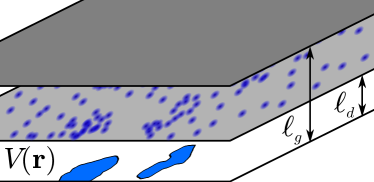
For definiteness we consider -type doping from here on. In the experimental setup donors are located in a layer separated from the quantum well by a spacer of width (see Fig. 9). Donors of average density induce a random potential in the quantum well. It creates puddles by attracting carriers to those regions where the conduction band lies below the Fermi level. Ignoring the screening of by these localized carriers, we have
| (124) |
where lies in the plane of the heterostructure and the last term comes from the induced charge on the gate electrode, located a distance from the quantum well; , see Fig. 9. We denoted the dielectric constant by and the donor charge density by . Taking the latter to be -correlated with variance , we get
| (125) |
where and .
We will now estimate the puddle parameters. At full depletion the density of puddles depends on the ratio of and . We define the characteristic density of donors,
| (126) |
at which .
At high donor densities the band edge fluctuates heavily and dips frequently below the Fermi level. This limit is beyond the scope of this work, since inter-puddle tunneling can lead to and bulk conductivity , corresponding to a symplectic metallic phase rather than to a topological insulator.Fu and Kane (2012) We leave out an estimate of since it depends strongly on the experimental parameters.
Let us next consider low donor density, , so that puddles can be made rare and small by adjusting the Fermi level a distance below the conduction band edge. Bulk conductivity is then activated in nature. If temperature is low enough, conduction can become dominated by the edges. Our next goal is to estimate the puddle density and the mean level spacing . In our analysis we closely follow Ref. Gergel’ and Suris, 1978.
The gate electrode is separated from the quantum well by a distance . Because of screening of the donors by the gate, the potential is correlated in the quantum well on the same length scale . Puddles occur in rare regions of size , where the potential fluctuation exceeds the value . The typical value by which a rare fluctuation exceeds is obtained to leading order in from the distribution [we ignore the logarithm in Eq. (125) considering and of the same order of magnitude]. We get
| (127) |
The carriers in the quantum well form a puddle of area to smoothen out the dip caused by the donor density fluctuation. Since , we approximate the Dirac spectrum by quadratic dispersion with mass (see also the beginning of Section IV). Assuming weak interaction, , we may use the Thomas-Fermi approximation for the description of the puddle, . Therefore the electron density in the puddle is . Denoting by the number of electrons in the puddle, their total electrostatic potential is , assuming . This potential should compensate for the potential fluctuation, . Using, in addition, the above-mentioned Thomas-Fermi estimate of , we find the puddle linear size , where is the effective Bohr radius. Finally, since , we get
| (128) |
The last relation is obtained from Eq. (70) using our assumption of small puddles, . The puddle has a large number of electrons if (which we have assumed throughout this work, except for the qualitative discussion in Section II). Taking a nearly ballistic dot, where the Thouless energy , we can finally estimate .
These are properties of a single puddle. To assess the puddle density , we first note that the distance to the gate is an effective screening radius, and we can divide the quantum well into regions of area between which the potential is uncorrelated. Puddles occur in those rare places where the local potential fluctuation exceeds the value . The probability for this to happen is exponentially small, , as follows from the distribution . The total carrier number of puddles in the square compensates for the corresponding fluctuation in the donor number, . Since only a fraction of the uncorrelated regions contains puddles, we obtain the puddle density
| (129) |
In Eq. (124) above we ignored the screening of potential fluctuations by the electron density due to puddles. This density is to be compared with the typical fluctuation of the donor density on lateral scale (the charge induced on the gate electrode smears out fluctuations on scales larger than ). Therefore the condition to ignore screening by carriers is . Using the relation [see Eq. (126)] with Eqs. (128) and (129) we see that the condition is , which is consistent with our assumption of weak doping, .
Finally, the bulk conductivity caused by rare puddles is negligible. The puddle-to-puddle hopping conductivity is proportional to the tunneling probability times the thermal activation factor (we used and denoted the penetration depth of the electron wavefunction into the bulk). Both of these factors are small at temperatures , making it very difficult for edge electrons to find a percolation path through the bulk. These reasons make the low-temperature bulk conductance negligible compared with the conductance of the edges, even if the latter one is reduced by inelastic backscattering. Next, we estimate the resistivity of the edges induced by the backscattering of edge electrons by nearby puddles.
V.2 Resistivity of a long edge
We are now in a position to assess the applicability of the single-dot theory developed in Sections III and IV to charge puddles created by random fluctuations of the donor density. First of all, we used RMT for dots with electrons. The Thomas-Fermi approximation utilized in derivation Eq. (128) also assumes . This assumption is met in the rare-puddles limit () only if while . Second, Sections III and IV consider the limits of and , respectively, while Eq. (128) predicts for random puddles of charge. Therefore, the random-puddles case is on the border-line of the descriptions developed in the aforementioned sections. In the following, we perform edge resistivity estimate in two limits conforming with the assumptions of Sections III and IV, respectively. We will then identify, which of the model-based conclusions hold under the realistic conditions described by Eq. (128).
V.2.1 Resistivity of a long edge in the absence of charging effects
The single-dot backscattering in the absence of charging effects, , was discussed in Section III. There, in deriving Eqs. (39) and (40), we replaced the dot level widths by their average values. This is what the conductance correction from a typical puddle would be. To assess the conductance of a long edge with many puddles, we need to average over the distribution of level widths. In the case of a long edge, there can be rare instances of exceptional puddles which produce most of the backscattering. This can be seen from Eq. (37) at low temperatures, , when level 1 is close to Fermi energy, . (Here is measured from the Fermi energy.) Averaging Eq. (37) over dot parameters, at fixed peak position and width , leads to 666The second term in Eq. (39) was obtained from Eq. (130) by replacing , which, however, we will not do here
| (130) |
In absence of charging effects the gate-voltage averaged conductance correction, , is dominated by the peaks, as indicated by strong -dependence in Eq. (130). Therefore at low temperatures , we obtain by averaging Eq. (130) over the peak position , and the width of the resonant level. For the latter, we use the symplectic Porter-Thomas distributionHaake (2010) . We then find from Eq. (130),
| (131) |
The integral over in Eq. (131) can be done first and is dominated by . The remaining integral over is dominated by , since the integrand becomes large for small level widths. We see that most of the backscattering at low temperatures is caused by rare quantum dots with rather than typical ones with . This was not captured in Eq. (39), which describes typical dots.
The corresponding high-temperature limit is given in the first term in Eq. (39), and there the average over level width is trivial. Combining the limits of low and high temperatures, we get from the first term in Eq. (39), and Eq. (131)
| (132) |
Since the average level width depends on the distance between the dot and the edge, the above equation gives the conductance correction due to a puddle at a fixed distance from the edge.
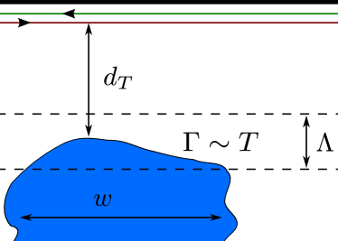
To estimate the long-edge resistivity , we will sum over the single-puddle corrections . Let us first consider an edge with just one puddle contributing to the edge resistance . Then where , and is a small resistance introduced by the puddle. On a long edge multiple puddles contribute to the edge resistance, yielding , where the sum is over all puddles, labeled by the index . Since scattering off puddles is inelastic and incoherent, the long edge is characterized by a self-averaging resistivity. Denoting the edge length by , we then have
| (133) |
We introduced the density of puddles [see Eq. 129] in converting the sum over the puddle positions into a two-dimensional integral. Since is independent of the position along the edge [see Eq. (132)], the integral over the length canceled against the pre-factor . The remaining integral over edge-dot distances, across the width of the sample, was converted into an integral over the average level width . The level width decays exponentially in the distance between the edge and the dot, , where is the penetration depth of the electron wave function into the bulk.
V.2.2 Resistivity of a long edge in the Coulomb blockade regime
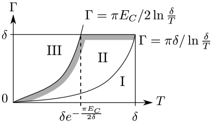
We will next calculate the long-edge resistivity in the limit of large charging energy, . The main contribution to the resistivity comes from puddles with an odd number of electrons. In those puddles the average of over level widths is dominated by their typical values, (unlike in the previous subsection). Therefore, Eqs. (117), and (121)–(123) give the conductance correction averaged over dot parameters and gate voltage, for a fixed edge-dot distance . To find the long-edge resistivity, we need then to sum over possible distances. As explained in the end of the previous subsection, this sum can be converted into an integral over the average level width . This integral is given by Eq. (133) which is applicable also here, in the presence of large charging energy. However, the integration over is more involved than in the previous subsection. We detail the integration in Fig. 11.
At temperatures , the integration domain can be divided into two regions (I and II, see Fig. 11) where is given by Eqs. (117) and (120), respectively. The shaded part in region II, where , gives the main contribution to the integral. Using Eq. (121) in Eq. (133) we find then
| (135a) | |||
At lower temperatures , Eq. (120) is no longer applicable up to , but only up to the smaller value , and region II shrinks accordingly, see Fig. 11. Still, the main contribution to Eq. (133) comes from the upper end of this region, described by Eq. (121). We find
| (135b) |
which matches with Eq. (135a) at .
We see that in the Coulomb blockade case at any , the resistivity of a long edge is weakly dependent on temperature, see Eqs. (135a)-(135b). This is because most of the resistance originates from puddles with an odd number of electrons. In those puddles the ground state degeneracy induces a logarithmic-in- helical edge resistivity for a wide range of temperatures.
The presence of odd-electron-number puddles is probable even if the strong inequality between the charging energy and level spacing is broken and even if the number of electrons in a puddle is not large, i.e., if and . In this case, we expect the anisotropy of the “bare” exchange integral to become . Taking into account that is also never a large parameter, we arrive at the following estimate of edge resistivity
| (136) |
at low doping, , see Eq. (126). This result was included in Section II, see Eq. (19). Equations (135a), (135b), and (136) above differ from that given in Ref. Väyrynen et al., 2013, where , since there the odd-occupied puddles were not accounted for.
VI Analysis of existing experimental data
In this section we connect our theory with existing experiments in HgTe and InAs/GaSb quantum wells. We start by calculating the characteristic donor density and the density of puddles for HgTe quantum wells. Considering a well of thickness , one has König et al. (2008) and . With a dielectric constant König et al. (2013) , we find . Ignoring the logarithm in Eq. (126), we get the characteristic donor density . The doping density in Ref. König et al., 2007, , was somewhat higher than the above value. If the sample of Ref. König et al., 2007 would be in the bulk-metallic phase, we would expect a high bulk conductivity, Fu and Kane (2012) . However, this is not what was observed: the measured conductance of a long sample with dimensions was , giving an upper bound for bulk conductivity, , and indicating an insulating bulk. Therefore it seems that the samples of Ref. König et al., 2007 are near the transition to symplectic metal phase, Fu and Kane (2012) but still on the topological-insulating side of it, as the nonlocal transport Roth et al. (2009) and direct measurements of the current distribution in the sample Nowack et al. (2013) indicate.
Our analysis of Subsection V.1, which assumed , is strictly speaking not valid near the transition. However, in estimating the puddle density, we can still use Eq. (129) by extrapolating to the crossover density, . This leads to . Using König et al. (2007) , and , we find 777 Note that , contrary to the assumptions of Eq. (129). The smaller is, the more effective is the screening of the potential fluctuations that create the puddles. In the limiting case of shorter than the radius of “deep” states with energies close to the center of the gap, the exponent in Eq. (129) is multiplied by an additional small factor . We believe, however, that we are only slightly overestimating by using here Eq. (129), as the heterostructures of Ref. König et al., 2007 are in an intermediate regime, . . Finally, using the wave function penetration depth , we obtain the number of near-edge puddles per unit length, . Therefore it is unlikely that multiple puddles would exist near the edge in short samples of length . This allows us to explain the approximate quantization of conductance observed in samples with . We may associate the deviation of from the universal value with electron backscattering off a single, or at most a few, puddles. Furthermore, the observed König et al. (2007) rapid fluctuation in the dependence of on gate voltage may be related to the sweeping of the chemical potential over the discrete electronic levels of a puddle.
In short samples ( for the parameters of Ref. König et al., 2007) the theory of backscattering off a single puddle developed in Subsection II.0.1 becomes relevant. We showed that at low temperatures () the puddle-induced correction to the edge conductance displays strong dependence on gate voltage (see Fig. 2a). This dependence comes from charging the puddle with electrons one by one. The gate voltage increment corresponding to the addition of an electron is where is the gate-puddle capacitance. Replacing by the puddle total capacitance , we have , where is the puddle charging energy. From Eq. (128) we have so that . This is a lower estimate for since, by replacing with , we ignored screening by other puddles and by the helical edges. Indeed, from Ref. König, we estimate a higher value, . More importantly, our theory predicts the temperature dependence of the helical edge resistance . The increase of the resistance above the single-edge universal value is related to evaluated in Subsection II.0.1, . Note that maxima in backscattering correspond to maxima in the resistance. At , the maxima and average value of depend weakly on temperature over a broad temperature interval [see Eqs. (7), (114), (117)]. This is in contrast with the minima of which obey a stronger ( power-law) dependence, see Eqs. (5) and (107). The amplitude of fluctuations, , decays with increasing temperature. The temperature scale above which fluctuations become suppressed is the puddle charging energy, which typically is of the same order of magnitude as level spacing, , see Eq. (128). While there is no detailed measurements of temperature dependence of resistance in short samples, it has been established that the resistance fluctuations decrease with temperature. König et al. (2007); König ; Eikenberg et al. (2014) However, the suppression of fluctuations with increased temperature is not unique to the above mechanism due to puddles. For example, coherent backscattering off correlated spins may produce such a feature. Cheianov and Glazman (2013); Altshuler et al. (2013) Considering spinful puddles close to the edge, we can estimate the temperature scale , at which the puddle spins become correlated. Cheianov and Glazman (2013) Using and , we get , which is clearly an over-estimate, since we expect . Note also that the derivation of assumes the presence of at least two puddles near the edge, which may not be true in short samples.
Strong evidence for puddles was given in Ref. König et al., 2013, where the edge conductance was shown to be very sensitive to local gating. However, we cannot fully explain the single instance where the authors were able to completely suppress () conduction of an edge state. In our theory, an accidental large () puddle near the edge would give a conductance correction , see Eq. (16).
In long samples () multiple puddles may lie near the edge, leading to resistance scaling linearly with sample length, . Experiments with HgTe samples of show a strongly reduced edge conductance, König et al. (2007); Nowack et al. (2013) or resistive behavior. Gusev et al. (2014) In long samples the current carried by edge modes may start to leak into the bulk. Väyrynen et al. (2013) This happens in samples longer than the leakage length , where is the bulk conductivity and the edge resistivity. In Ref. Nowack et al., 2013 the authors showed that the current was carried by the edges in the topological state, despite the inferred high edge resistance at . Using the estimated bulk resistance , and the sample dimensions , we obtain , while the edge resistivity is . This leads to leakage length , in agreement with low leakage found in Ref. Nowack et al., 2013. Finally, we can estimate the theoretical value for puddle-induced resistivity , by calculating the pre-factor in Eq. (136), . Taking Nowack et al. (2013) and using our previously calculated values and , we find . This leads to and . Our estimate , which is about 6 times higher then the actual , is reasonably close to the measured value, considering the probable overestimation Note (7) of .
The temperature dependence of long edge resistance has been studied in HgTe, Nowack et al. (2013); Gusev et al. (2014) as well as in Si-doped topological InAs/GaSb quantum wells. Spanton et al. (2014); Du et al. (2013) In the latter system Ref. Du et al., 2013 finds a temperature-independent resistance over three decades of temperatures, up to . This is somewhat at odds with our predicted dependence at low temperatures, , see Eq. (136). Measurements at higher temperatures, Spanton et al. (2014) , in the same system show very little -dependence in edge resistance. In HgTe, the resistance at has been measured, and its observed -dependence seems to indicate an onset of activated bulk conduction. Nowack et al. (2013); Gusev et al. (2014) Using the parameters of Ref. König et al., 2007, we find , which makes it possible that in these experiments. Thus, to definitely support or rule out the existence of puddles, experiments at lower temperatures, , are needed. In the next, concluding section, we summarize the predictions for the low-temperature resistance induced by puddles.
VII Conclusions
We have shown in the previous section how several key measurement results are explained qualitatively by the puddle physics. The explained features include the high resistance of the helical edges in long samples and the fluctuations of the excess resistance in short ones. However, we are not aware of detailed low-temperature data which would allow quantitative comparison with the theory developed in this paper. In this section, we will summarize the predictions for the resistance at low temperatures .
We will start by considering a single puddle with relatively large charging energy, . Such a puddle may be found in short samples (, using the parameters of Ref. König et al., 2007), or perhaps even formed intentionally. König et al. (2013) Either way, the resulting puddle-induced edge resistance at low temperatures () will display very distinct dependence on the temperature and gate voltage. (Here is the deviation of edge resistance from the universal value .) Plotted against gate voltage, the resistance displays narrow peaks separating valleys, see Fig. 2. The resistance strongly depends on the parity of electron number in the puddle, and therefore is very different in neighboring valleys. When the puddle occupation is even, the puddle-induced resistance is small and decays fast, , towards the universal value, see Eq. (5). When the occupation is odd, however, the decay is slow, , see Eq. (14). This slow decay persists over a broad interval of temperatures, down to . (Here is the width of electron level in a puddle; reaches its maximum, , when the puddle is very close to the edge.) Only at very low temperatures, below , do we have throughout an odd valley, see Eqs. (5) and (15). In the peaks between the valleys, is approximately independent of temperature at [see Eq. (7)], and has the aforementioned power-law-dependence at lower temperatures, see Eq. (6). Combining the above description of peaks and valleys, we finally note that the amplitude of fluctuations in decreases with increasing temperature, while the gate-voltage-averaged grows.
As we argued in Subsection V.1, in a typical doping-induced puddle we have . The signatures illustrated by Fig. 2 remain valid. We must note, also, that if the puddle is very close to the edge, , then the slow -dependence, , in the odd-occupied valleys may not persist over a broad temperature interval.
On a long edge, there are always puddles far from the edge. Such remote puddles with an odd electron number dominate the low-temperature resistivity of a long edge. Taking , as is appropriate for doping-induced puddles, we find resistivity , see Eq. (19). This result is valid at temperatures below the average level spacing, . The logarithmic temperature-dependence of is one of the main testable predictions of this paper.
Acknowledgements.
We thank Katja Nowack for discussions. This work was supported by NSF DMR Grant No. 1206612, U.S.-Israel Binational Science Foundation (Grant 2010366), the Simons Foundation, and the Bikura (FIRST) program of the Israel Academy of Science. LG is grateful to the Aspen Center for Physics, supported by NSF Grant No. PHYS-106629, for hospitality which helped to complete this work.Appendix A Tunneling through an extended edge-dot contact
In the main text of this work we assumed a point-contact model for the tunneling between the helical edge and the quantum dot. That led us to momentum-independent, diagonal (in the Kramers index) tunneling matrix elements in the Hamiltonian (20). The goal of this section is to demonstrate that our main conclusions remain valid for an extended edge-dot junction. First, we explicitly show below how TR symmetry enforces reflectionless edge transport, at any electron energy, if there is no interaction inside the dot. Next, in Subsection A.1, we include interaction, and show that in the low-temperature limit the backscattering correction to the conductance remains universal, . Finally, we compare the conductance corrections from quantum dots with extended and point-like contacts. We find that dots with an extended contact yield a smaller correction to the conductance than those coupled to the edge by a point-contact.
We start by introducing the most general tunneling Hamiltonian,
| (137) |
The matrix elements of satisfy the relation dictated by TR symmetry,
| (138) |
The tunneling matrix elements form a matrix in the Kramers indices . We can diagonalize this matrix and make its elements real in the diagonal basis by performing a unitary transformation of the dot states. Introducing phases , we can write . Then the diagonalizing unitary transformation reads
| (141) | |||
| (146) |
This rotation generally depends on . If is independent of (tunneling through point-contact), as assumed in the main text, the rotation puts the Hamiltonian in the simple form of Eq. (20)
| (147) |
with .
In this form, the two complementary components of the Kramers doublets for any level are coupled to the respective channels , ; there are no dot states which couple simultaneously to and . Clearly, the Hamiltonian (147) does not lead to backscattering. In the general case of Eq. (137) the unitary transformation (146) does not lead to such decoupling. Nevertheless, TR symmetry forbids elastic backscattering, as we will demonstrate next.
The rate of transition from an initial state to a final state is
| (148) |
where is the thermal probability factor of state . The -matrix is defined as
| (149) |
where is the unperturbed Hamiltonian, and , Eq. (137), is the pertubation. Without interaction, the unperturbed Hamiltonian in Eq. (149) is
Consider first backscattering of a single electron. We will denote the initial and final states as single-particle excitations over some common vacuum state, and . From the TR symmetry of the Hamiltonian and the perturbation , it follows that also the -matrix is TR-symmetric. Therefore we have . Since energy is conserved, , the amplitude vanishes,
| (150) |
Similarly, the backscattering amplitude of non-interacting many-particle states vanishes.
A.1 Backscattering in the constant-interaction model
In this section we will show that even in the constant-interaction model there is backscattering if the edge-dot tunneling contact is extended. We will also compare the resulting conductance correction, , to the one due to a quantum dot point-contact-coupled to the edge. It is found that generally a point-like edge-dot junction gives rise to a larger correction to edge conductance.
The simplest interacting model for the dot is the Anderson-type Hamiltonian of a single level,
| (151) |
where and is above the Fermi level so that the level is empty in its ground state. We will consider low temperatures at which transport through the level is dominated by virtual processes. Using the -matrix approach, we will calculate the backscattering current ,
| (152) |
where the sum is over initial and final states ( and ), is the number of backscattered particles, and is the -matrix fourth order in tunneling, Eq. (149). Assuming that the level is empty in the initial and final states, we have two contributions to the -matrix,
| (153) |
where
| (154) | ||||
| (155) | ||||
| (156) |
The term corresponds to a process where at most one virtual electron occupies the level at a given moment. The second term has a virtual intermediate state where the level is doubly occupied and therefore the second denominator in Eq. (155) is of order . In the non-interacting limit these two processes cancel each other and the amplitude for backscattering vanishes. Considering a final state (we assume unequal momenta and conserved total energy), the amplitudes for these two processes are
where
(Note that vanishes if the tunneling amplitude is independent of momentum.) Accounting only for the above 1-particle backscattering process, correction to ideal conductance from Eq. (152) becomes,
| (157) |
At low energies we can expand the tunneling amplitudes in energy. In particular,
The conductance correction at low temperatures becomes (we drop from the subscript indicating backscattering of one particle)
| (158) |
in agreement with the general result (see Section II).
The derivative in Eq. (158) introduces a length scale , which can be interpreted as the size of the tunneling region. We will next find out how large has to be, in order to yield comparable to that given by a point-contact-coupled quantum dot.
To get a rough estimate, we write , and introduce the level width . We also denote , to ease the comparison to a Coulomb blockaded dot, discussed in Subsection II.0.1. In the limit of large charging energy, the virtual double-occupied dot states are rare, and we have . Then Eq. (158) becomes
| (159) |
The conductance correction due to a dot identical-to-above, but with a point-like contact to the edge, is given in Eq. (5). From Eq. (159), comparing with the point-contact result Eq. (5), we see that only if the tunneling region is large enough, , where is the dot Thouless time. The Thouless time is the diffusion time of electron across the dot, and therefore always larger than the ballistic crossing time , being the dot linear size. Since also , we find , i.e., junction has to be wider than the dot linear size. This is a justification for using a point-contact coupling between the edge and the dot in the main text.
Appendix B Averaging over disorder
In this section, we show how to obtain some of the averages used in the main text. In particular, in Subsection B.1, we calculate the average matrix element of the non-universal interaction . We show that for screened Coulomb interaction . In Subsections B.2 and B.3, we show how to obtain the RMT averages over the dot energy levels cited in the main text, in Sections III and IV.2, respectively. The RMT averages used in Subsection IV.1 are given later, in Appendix E.
B.1 Average of the non-universal part of interaction
In this subsection we give the typical value of the (squared) backscattering matrix elements of the interaction . The backscattering matrix elements are given by the off-diagonal, non-universal part of the intra-dot interaction. In this subsection, we denote this off-diagonal part by . (The same convention is followed in Section IV, where the special notation is reserved for the diagonal part.) Note that in the symplectic ensemble 888We use the symplectic ensemble since a generic single-particle Hamiltonian of the dot does not conserve any component of the electron spin (i.e., the spin scattering rate is larger than the level spacing, ). all the backscattering matrix elements are on average equal. Using the standard diagrammatic approach, Aleiner et al. (2002) we find,
| (160) |
Here denotes average over dot levels, is the dot density of levels, is the area of the dot, denotes average over the Fermi surface, and is the Fourier-transform of the interaction potential . The sum is over the eigenvalues of the diffusion operator with Neumann boundary conditions. The lowest non-zero eigenvalue is the inverse time to diffuse through the system (Thouless energy), and gives the dimensionless conductance of the dot, . Introducing a shape-dependent coefficient we can write in Eq. (160). For the special but realistic case of screened Coulomb interaction the zero-momentum component dominates, , and we find
| (161) |
B.2 Averages over dot energy levels in Section III
In this subsection we show how to average over the level sums in Eqs. (32), (35), and (37), to obtain Eqs. (39) and (40) of the main text. Our main tool in averaging over dot energy levels is the -point correlation function defined as
| (162) |
where the brackets denote average over disorder, and the primed sum is taken over all unequal levels. Therefore vanishes if any of the coordinates coincide, which is a manifestation of level repulsion. The correlation functions are known from RMT.Mehta (2004) For us, the most important correlation function is the 2-point function . Its asymptotic behavior for matching arguments is when , while distant levels are uncorrelated, as . Here for Gaussian orthogonal, unitary, and symplectic ensembles, respectively. Due to the strong spin orbit coupling in the topological insulators, we use the symplectic ensemble throughout. Note (8) The higher order correlation functions behave similarly.
The numbers and in Eqs. (39) and (40) are given by
| (163) | ||||
| (164) |
These averages can be calculated using the correlation functions . Note that in Eqs. (39) and (40) we have the extra condition that level is excluded from the sum, i.e., none of the levels summed over is at the Fermi energy. For example, we then get
| (165) |
We leave out evaluation of the level sum , since it requires, for example, integration of the 6-point function . In principle, can be evaluated similarly to .
B.3 Averages over dot energy levels in Subsection IV.2
In this section we derive from Eq. (106) the disorder-averaged conductance correction, Eq. (107), due to 1-particle backscattering in the even Coulomb blockade valley. The averages over dot levels are evaluated in similar fashion as in the previous subsection B.2.
The main contribution to the sum over levels in Eq. (106) comes from all levels unequal. Dispensing with numerical pre-factors, we get from Eq. (106)
| (166) |
where the dimensionless factor is
The high-energy cutoff on the level sum, , makes dependent on . The main contribution to comes from unequal levels, i.e., unequal in the sum. Since we are not interested in the pre-factors, we will only demonstrate that . For example, the last term gives
| (167) |
where , and we changed variables . To leading order in , we can replace the two-point correlator [Eq. (162)] by one, . The remaining integral gives to leading order
| (168) |
Inserting this into Eq. (166) leads to Eq. (107) of the main text.
Appendix C An exactly-solvable toy-model with arbitrary interaction strength
In this section we derive the substitution, Eq. (46), used in Subsection III.2. To account for the intra-dot interaction exactly, we use the -matrix formalism. This amounts to replacing in the cross section, in Eq. (26), the interaction matrix elements by those of the -matrix, . Here is the two-particle Green function of non-interacting electrons. At high enough temperatures where direct tunneling dominates (which is the case when Eq. (43) is valid), we consider only diagonal parts of the single-particle Green functions, see Eq. (29). Then the two-particle Green function takes the form
Let us consider a toy-model of only two dot levels, and , and an interaction that allows only 2-particle backscattering, . We want to calculate the matrix element . In the basis (we can neglect doubly occupied levels since they are always annihilated by ) the matrix for is proportional to unit matrix (and for our purposes can be treated as a scalar), while
| (169) |
The inverse is easily calculated and the element of the -matrix corresponding to two-particle backscattering becomes,
| (170) |
In resonant tunneling, Eq. (42), we have and thus . Inserting this in Eq. (170) leads to Eq. (46).
Appendix D Derivation of Eq. (106)
In this section, we discuss the conductance correction in the even valley of a Coulomb blockaded quantum dot at low temperatures. We present the detailed derivation of , Eq. (106), due to backscattering of one particle, and show how inclusion of two-particle backscattering modifies the result. We also give the relative importance of different terms in the 5th order -matrix, see Table 2.
As explained in Subsection IV.2 of the main text, in the even valley the main contribution to the -matrix comes from the 12 terms with small denominators (independent signs). These terms are the elements in rows 1, 3, and 6 in Table 2. In particular, the third elements in each of the rows 1 and 6, and third and fourth elements of the row 3, were used in the example in the main text, Eq. (105). The transition amplitude between states and induced by the 12 terms from rows 1, 3, and 6, of Table 2 is
| (171) |
where and
| (172) |
where . Since the dot has an even number of electrons in its ground state, and we are at low temperatures , we used a zero-temperature distribution function for the dot states: , level 1 being the lowest unoccupied level. We can now evaluate the contribution , due to two electrons in Kramers states scattering into states , to the total backscattering current. The partial current is a sum (over the initial and final states) of the transition rates from state to the final state . Equation (73) relates the rate to the amplitude in Eq. (171). Summing over the initial states and the final state momenta , we find
| (173) |
The distribution functions are the result of summing the factors over initial states with weight . The correction to the ideal current is then
| (174) |
where counts the number of backscattered particles. [Naturally, Eq. (174) consists of contributions arising from backscattering of both one and two particles.] The above Eq. (174) is a generalization of Eq. (27) to the case of a Coulomb blockaded quantum dot in the even valley.
Let us next consider the contribution to due to 1-particle backscattering. From Eq. (172) one sees that because is symmetric under time-reversal, is the same for all combinations that backscatter one particle. At low temperatures we can expand the denominators of for small which brings out a factor , leading to as in the case without charging interaction, Eq. (32); see also the amplitude Eq. (4) and its derivation. Linearizing the Fermi functions in Eq. (174) in bias voltage, leads to Eq. (106) given in Subsection IV.2.
The conductance correction due to 2-particle backscattering is obtained similarly from Eq. (174). We find
| (175) |
From Eq. (175), comparing to Eq. (106), we see that at low temperatures.
D.1 2-particle contribution near the peak
In this section we show how 2-particle backscattering modifies the ideal conductance in the even valley near the peak, where and level 1 is the lowest unoccupied level. The 1-particle contribution was given in Eqs. (110) and Eq. (112), calculated in Subsection IV.2.2.
For backscattering of two particles, we set in the amplitude, Eq. (108). Summing the rates, Eq. (73), leads to
| (176) |
The integrals are performed the same way as in Subsection IV.2.2. In the low-temperature limit, , we find
| (177) |
Compared to the 1-particle backscattering contribution, Eq. (110), is smaller by a factor .
Appendix E Components of the exchange tensor and averages in Subsection IV.1
In this section we give the components of the exchange tensor , introduced in Eq. (79) of Subsection IV.1, in terms of microscopic dot parameters. We will also calculate the disorder-averaged odd-valley conductance correction in Subsection E.1. This requires averaging over the proper exchange couplings .
The components can be obtained by using the microscopic dot Hamiltonian [given in Eqs. (71)–(72)] in Eq. (76) and matching terms with Eq. (77).
For the isotropic part we find
| (179) |
The first term in is independent of interaction and corresponds to the exchange coupling of the usual Anderson Hamiltonian. The components [see Eq. (79)] are given in Table 1.
E.1 Averages in Subsection IV.1
In this subsection we obtain the disorder-averaged conductance correction in the odd Coulomb blockade valley, Eqs. (103a)–(103c) of Subsection IV.1.4.
In Eq. (98) we expressed in terms of the bare exchange tensor components . The conductance correction takes the simple form
| (180) |
if we write , , , and . From Table 1 we find
| (181a) | ||||
| and | ||||
| (181b) | ||||
with .
Averaging the terms and in Eq. (180) over disorder is straightforward and follows Subsection B.2. However, due to the large number of different terms we will settle with an order of magnitude estimate.
Let us first consider the behavior near the peak, and take . Then one easily finds
| (182) |
Next we take . Then
| (183) |
where are numerical coefficients, and where we have introduced the averages ()
| (184a) | ||||
| (184b) | ||||
| (184c) | ||||
As long as , the largest sums are and . To leading order in ,
| (185) |
Keeping only the terms and in Eq. (183) leads to Eq. (103b) of the main text. Closer to the bottom of the valley, , the sum of the logarithmic terms in in Eq. (183) above becomes subleading. The main contribution to Eq. (183), and , comes from the terms of the order of in the sums , , , . This leads to Eq. (103c) of the main text.
Appendix F Renormalization group for the anisotropic Kondo model
We saw in Subsection IV.1.4 of the main text that in the odd valley the correction to the conductance, , arises due to anisotropy in the exchange coupling. In this section we study, using perturbative renormalization group, how the weakly anisotropic Kondo model, Eq. (77), flows to the isotropic fixed point at low energies. Anderson (1970) We find that the renormalization leads to a logarithmic suppression of as one approaches low temperatures , see Eq. (99).
In Subsection IV.1 we derived the Hamiltonian for the effective interaction between the helical edge and a quantum dot with spin, valid at temperatures ,
| (186) |
The first term in Eq. (186) corresponds to the free itinerant electrons of the helical edge. The sum over momenta is restricted to a band of energies , and we set . The edge spin density at the point contact is denoted , while is the spin-1/2 operator of the dot. We have explicitly indicated the cutoff-dependence of the exchange couplings .
Next, we will follow Ref. Anderson, 1970 and eliminate the high-energy states in a small strip of width near the edge of the band, thus reducing the cutoff energy to . The resulting low-energy Hamiltonian contains information about the rare virtual transitions between the low- and high-energy sectors. Considering only the exchange part of this low-energy Hamiltonian, we can relate its coupling constants to the couplings of the original Hamiltonian. To second order in the couplings this relation is
| (187) |
Here is the Levi-Civita symbol. Let us assume that is almost isotropic, , where the anisotropic part is traceless and symmetric (trace would add to the isotropic part , and antisymmetric part corresponds to a rotation of ). Taking to be small, we can write the renormalization group equations to linear order in ,
| (188a) | ||||
| (188b) | ||||
Solving the equation for gives the known result that flows to strong coupling at low energies,
| (189) |
The Kondo temperature is invariant under reduction of the cutoff . The anisotropic perturbation flows towards zero upon reduction of bandwidth from to ,
| (190) |
Setting , Eq. (190) gives the logarithmic suppression of backscattering used in Eq. (99).
Appendix G Single-dot conductance correction at temperatures
In this section we consider the correction to the conductance at intermediate temperatures, , alluded to in Subsection IV.4 of the main text.
We will first discuss qualitatively the derivation of . For that, we follow the part of Section II devoted to the electron backscattering by the exchange interaction. The spin of the dot remains finite (albeit not equal to or ) even at . That allows us to relate the backscattered current to the time-averaged derivative of the -component of the total spin,
| (191) |
The number of electrons in a quantum dot is well-defined at . However, its spin is not determined by the electron number, if . That makes the spin transfer from the electrons of the edge to the electrons of the dot effective in the backscattering at any value of . Assuming the dot is “deep” in the Coulomb blockade regime, electrons can not tunnel into it. The backscattering then is governed by an exchange Hamiltonian of a form similar to Eq. (8),
| (192) |
Unlike Eq. (8), the form of Eq. (192) includes off-diagonal in the orbital index matrix elements of the total spin of the dot. That makes Eq. (192) applicable in the energy band and allows for an electron transition between the dot levels in the course of the edge electron scattering. At it is sufficient for us to keep only the largest, isotropic part of exchange [cf. Eq. (9)],
| (193) |
(Here and are the tunneling matrix elements for the dot levels and ; unlike in Eq. (9), we keep in the denominators of Eq. (193) only the charging energy, as we are not aiming here at the description of the Coulomb blockade peaks in ). Indeed, at , contrary to the low-temperature limit, the spin transferred to the dot in a backscattering event may relax due to the intra-dot scattering processes, see Subsection III.3.
The isotropic exchange Hamiltonian, Eqs. (192) and (193), commutes with the total spin, therefore . Here is the intra-dot interaction Hamiltonian which causes the relaxation of the dot spin, . In this way, we relate to the spin kinetics of the dot,
| (194) |
Here is the characteristic rate of the intra-dot electron relaxation at energy , cf. Eq. (49).
In the steady state, is determined by the balance between the above-mentioned intra-dot spin relaxation and transfer of the spin from the edge electrons due to the exchange interaction (192). In the absence of any intra-dot relaxation, the equilibrium with the edge would be reached at , assuming (this relation is derived similarly to the one for the limit considered in Section II). At , the rate of the spin transfer can be estimated as with being the analogue of the inelastic co-tunneling rate. Glazman and Pustilnik (2005) The rate balance equation for thus reads
| (195) |
Solving it and substituting the result in Eq. (194), we find for
| (196) |
The conductance correction scales with temperature as , with the coefficient depending on the ratio between the typical values of and .
Now we proceed with a more detailed derivation of . Since , it is convenient to use the average distribution function of the dot electrons, , introduced in Subsection III.3. (Here is the electron density of states in the dot.) In the absence of bias voltage, is independent of and equal to a Fermi function. Hereafter, we refer to it as the equilibrium distribution.
The correction to the ideal current is obtained from the number of backscattered, say, left-moving edge electrons per unit time. Electrons of the helical edge cannot tunnel into the dot at , and their scattering off the dot is mostly inelastic at (inelastic co-tunneling Glazman and Pustilnik (2005)). An inelastic scattering process leaves behind a particle-hole excitation in the dot. Accounting for the inelastic backscattering, we have
| (197) |
The second equality here follows from the fact that the co-tunneling process preserves the total number of electrons in the dot. The time-derivative is the the counter-part of the second term in Eq. (195) and contributes to the rate equation for the dot distribution function, as shown below.
The full rate equation for the distribution function consists of contributions from both co-tunneling and relaxation inside the dot,
| (198) |
(We neglect the contribution from direct tunneling, which is suppressed at temperatures .) The rate of intra-dot relaxation was evaluated in Eq. (55), see Subsection III.3. Considering a small deviation of from equilibrium distribution (i.e., a Fermi function), we have to linear order in the bias voltage ,
| (199) |
This is obtained from Eq. (49) in the limit of strong spin-orbit coupling (so that the integration kernel there cancels away). It is valid at , since we replaced averages of products by the products of averages when performing the averaging over dot levels, see Subsection III.3.
The backscattering current can be written in terms of the right-hand-side of Eq. (199) as we show next. In the steady state, we have in Eq. (198). Using Eqs. (198) and (199), we can then write in the form
| (200) |
Identifying , we see that Eq. (200) above is the analogue of Eq. (194) in the introduction to this section. To express in terms of known quantities, we will next solve for by using the steady-state version of Eq. (198). For that, we need to first write the equation analogous to Eq. (199) for the co-tunneling term in Eq. (198).
The co-tunneling term in Eq. (198) is evaluated using second order perturbation theory in tunneling or, equivalently, by using the Hamiltonian of Eq. (192) with given by Eq. (193). We find
| (201) |
The relation of Eq. (201) to the Hamiltonian (192) is evident since averaging over different dot levels there gives . Likewise, Eq. (201) is valid at temperatures less than the charging energy, . The distribution function of the edge electrons in Eq. (201) is .
To find the co-tunneling version of Eq. (199), we again consider a small deviation of from equilibrium. To the first order in bias voltage, we find from Eq. (201)
| (202) |
where we have introduced the inelastic co-tunneling rate ,
| (203) |
In the steady state, Eqs. (198), (199), and (202) yield the rate balance equation in the form
| (204) |
equivalent to Eq. (195). We find from Eq. (204)
| (205) |
Inserting Eq. (205) into the expression for , Eq. (200), we find the correction to the conductance,
| (206) |
Comparing to Eq. (66), we see that the result of Subsection III.3 remains qualitatively valid here. However, the tunneling rate there gets replaced by the co-tunneling rate here since, in presence of charging energy, direct tunneling (described by ) is strongly suppressed.
Evaluating the integral in Eq. (206) in the limiting cases of fast () and slow () co-tunneling, leads to
| (207) |
valid in the temperature interval . Here the first line corresponds to the case , where the slow intra-dot relaxation is the bottleneck for backscattering, and . In the second line the bottleneck is shifted to the co-tunneling process, and . Extrapolating towards low-temperatures, , the latter result can be written as where is the (disorder-averaged) isotropic part of exchange in Eq. (77) [see also Eq. (8)]. This is similar in form to the result in the odd valley, , see Eqs. (98) and (104). In the former case, however, the anisotropic part of exchange, , is not necessary for backscattering, since the dot spin relaxes fast in the intra-dot scattering processes.
References
- Kane and Mele (2005a) C. L. Kane and E. J. Mele, Phys. Rev. Lett. 95, 146802 (2005a).
- Kane and Mele (2005b) C. L. Kane and E. J. Mele, Phys. Rev. Lett. 95, 226801 (2005b).
- Bernevig et al. (2006) B. A. Bernevig, T. L. Hughes, and S.-C. Zhang, Science 314, 1757 (2006).
- Xu and Moore (2006) C. Xu and J. E. Moore, Phys. Rev. B 73, 045322 (2006).
- Wu et al. (2006) C. Wu, B. A. Bernevig, and S.-C. Zhang, Phys. Rev. Lett. 96, 106401 (2006).
- Budich et al. (2012) J. C. Budich, F. Dolcini, P. Recher, and B. Trauzettel, Phys. Rev. Lett. 108, 086602 (2012).
- Schmidt et al. (2012) T. L. Schmidt, S. Rachel, F. von Oppen, and L. I. Glazman, Phys. Rev. Lett. 108, 156402 (2012).
- Lezmy et al. (2012) N. Lezmy, Y. Oreg, and M. Berkooz, Phys. Rev. B 85, 235304 (2012).
- Kainaris et al. (2014) N. Kainaris, I. V. Gornyi, S. T. Carr, and A. D. Mirlin, ArXiv e-prints (2014), arXiv:1404.3129 [cond-mat.mes-hall] .
- Qi and Zhang (2011) X.-L. Qi and S.-C. Zhang, Rev. Mod. Phys. 83, 1057 (2011).
- König et al. (2007) M. König, S. Wiedmann, C. Brüne, A. Roth, H. Buhmann, L. W. Molenkamp, X.-L. Qi, and S.-C. Zhang, Science 318, 766 (2007).
- Gusev et al. (2014) G. M. Gusev, Z. D. Kvon, E. B. Olshanetsky, A. D. Levin, Y. Krupko, J. C. Portal, N. N. Mikhailov, and S. A. Dvoretsky, Phys. Rev. B 89, 125305 (2014).
- Du et al. (2013) L. Du, I. Knez, G. Sullivan, and R.-R. Du, ArXiv e-prints (2013), arXiv:1306.1925 [cond-mat.mes-hall] .
- Spanton et al. (2014) E. M. Spanton, K. C. Nowack, L. Du, R.-R. Du, and K. A. Moler, ArXiv e-prints (2014), arXiv:1401.1531 [cond-mat.mes-hall] .
- Liu et al. (2008) C. Liu, T. L. Hughes, X.-L. Qi, K. Wang, and S.-C. Zhang, Phys. Rev. Lett. 100, 236601 (2008).
- Väyrynen et al. (2013) J. I. Väyrynen, M. Goldstein, and L. I. Glazman, Phys. Rev. Lett. 110, 216402 (2013).
- Kouwenhoven et al. (1997) L. P. Kouwenhoven, C. M. Marcus, P. L. McEuen, S. Tarucha, R. M. Westervelt, and N. S. Wingreen, Proceedings of the NATO Advanced Study Institute on Mesoscopic Electron Transport E345, 105 (1997).
- Glazman and Pustilnik (2005) L. I. Glazman and M. Pustilnik, in Nanophysics: Coherence and Transport École d’été de Physique des Houches Session LXXXI, Les Houches, Vol. 81, edited by S. G. G. M. H. Bouchiat, Y. Gefen and J. Dalibard (Elsevier, 2005) pp. 427 – 478.
- Roth et al. (2009) A. Roth, C. Brüne, H. Buhmann, L. W. Molenkamp, J. Maciejko, X.-L. Qi, and S.-C. Zhang, Science 325, 294 (2009).
- Nozières and Pines (1999) P. Nozières and D. Pines, The theory of quantum liquids, Advanced book classics (Perseus, Cambridge, MA, 1999).
- Aleiner et al. (2002) I. L. Aleiner, P. W. Brouwer, and L. I. Glazman, Physics Reports 358, 309 (2002).
- Anderson (1966) P. W. Anderson, Phys. Rev. Lett. 17, 95 (1966).
- Note (1) This limitation is lifted if the tunneling region is extended, see Appendix A.
- Anderson (1970) P. Anderson, Journal of Physics C: Solid State Physics 3, 2436 (1970).
- Tanaka et al. (2011) Y. Tanaka, A. Furusaki, and K. A. Matveev, Phys. Rev. Lett. 106, 236402 (2011).
- Landau and Lifshitz (1980) L. Landau and E. Lifshitz, Statistical Physics, 3rd ed., Vol. 5 (Butterworth-Heinemann, 1980).
- Note (2) Using the equilibrium distribution is compatible with having different chemical potentials of the two fermion species due to the presence of the integral of motion .
- Bloch (1946) F. Bloch, Phys. Rev. 70, 460 (1946).
- Korringa (1950) J. Korringa, Physica 16, 601 (1950).
- van der Wiel et al. (2000) W. G. van der Wiel, S. D. Franceschi, T. Fujisawa, J. M. Elzerman, S. Tarucha, and L. P. Kouwenhoven, Science 289, 2105 (2000).
- Gergel’ and Suris (1978) V. A. Gergel’ and R. A. Suris, Zh. Eksp. Teor. Fiz. 75, 191 (1978), [Sov. Phys. JETP 48, 95 (1978)].
- Note (3) The lower limit is non-zero for a finite width sample where . Here we however assume a wide enough sample, so that the lower limit can be taken smaller than any other scale.
- Shklovskii and Efros (1984) B. Shklovskii and A. Efros, Electronic properties of doped semiconductors, Springer Series in Solid-State Sciences (Springer, Berlin, 1984).
- Note (8) We use the symplectic ensemble since a generic single-particle Hamiltonian of the dot does not conserve any component of the electron spin (i.e., the spin scattering rate is larger than the level spacing, ).
- Sivan et al. (1994) U. Sivan, Y. Imry, and A. Aronov, EPL (Europhysics Letters) 28, 115 (1994).
- Altshuler et al. (1997) B. L. Altshuler, Y. Gefen, A. Kamenev, and L. S. Levitov, Phys. Rev. Lett. 78, 2803 (1997).
- Note (4) For example, for HgTe with , , and one finds Gusev et al. (2014) .
- Hewson (1997) A. C. Hewson, The Kondo problem to heavy fermions (Cambridge University Press, 1997).
- Nozieres (1974) P. Nozieres, Journal of Low Temperature Physics 17, 31 (1974).
- Note (5) This is the gate voltage at which the lowest energy excitation of the dot changes between one with charge and one with spin. The nature of these excitations defines the form of denominators in the perturbative result for , see Eq. (81) and Table 1 of Appendix E.
- Knap et al. (2014) M. Knap, J. D. Sau, B. I. Halperin, and E. Demler, ArXiv e-prints (2014), arXiv:1405.0277 [cond-mat.mes-hall] .
- Fu and Kane (2012) L. Fu and C. L. Kane, Phys. Rev. Lett. 109, 246605 (2012).
- Note (6) The second term in Eq. (39) was obtained from Eq. (130) by replacing , which, however, we will not do here.
- Haake (2010) F. Haake, Quantum signatures of chaos, Vol. 54 (Springer, 2010).
- König et al. (2008) M. König, H. Buhmann, L. W. Molenkamp, T. Hughes, C.-X. Liu, X.-L. Qi, and S.-C. Zhang, Journal of the Physical Society of Japan 77, 031007 (2008).
- König et al. (2013) M. König, M. Baenninger, A. G. F. Garcia, N. Harjee, B. L. Pruitt, C. Ames, P. Leubner, C. Brüne, H. Buhmann, L. W. Molenkamp, and D. Goldhaber-Gordon, Phys. Rev. X 3, 021003 (2013).
- Nowack et al. (2013) K. C. Nowack, E. M. Spanton, M. Baenninger, M. König, J. R. Kirtley, B. Kalisky, C. Ames, P. Leubner, C. Brüne, H. Buhmann, et al., Nature materials 12, 787 (2013).
- Note (7) Note that , contrary to the assumptions of Eq. (129). The smaller is, the more effective is the screening of the potential fluctuations that create the puddles. In the limiting case of shorter than the radius of “deep” states with energies close to the center of the gap, the exponent in Eq. (129) is multiplied by an additional small factor . We believe, however, that we are only slightly overestimating by using here Eq. (129), as the heterostructures of Ref. \rev@citealpnumkonig07 are in an intermediate regime, .
- (49) M. König, Ph.D. thesis.
- Eikenberg et al. (2014) N. Eikenberg et al., (2014), unpublished.
- Cheianov and Glazman (2013) V. Cheianov and L. I. Glazman, Phys. Rev. Lett. 110, 206803 (2013).
- Altshuler et al. (2013) B. L. Altshuler, I. L. Aleiner, and V. I. Yudson, Phys. Rev. Lett. 111, 086401 (2013).
- Mehta (2004) M. L. Mehta, Random matrices (Elsevier/Academic Press, 2004).
| Term in -matrix | Denominator |
|---|---|
| , , | |
| , , | |
| , , , | |
| , , | |
| , | |
| , | |
| , , | |
| , | |
| , | |
| , | |
| , | |
| , | |