Forest resampling for distributed sequential Monte Carlo

Abstract: This paper brings explicit considerations of distributed computing architectures and data structures into the rigorous design of Sequential Monte Carlo (SMC) methods. A theoretical result established recently by the authors shows that adapting interaction between particles to suitably control the Effective Sample Size (ESS) is sufficient to guarantee stability of SMC algorithms. Our objective is to leverage this result and devise algorithms which are thus guaranteed to work well in a distributed setting. We make three main contributions to achieve this. Firstly, we study mathematical properties of the ESS as a function of matrices and graphs that parameterize the interaction amongst particles. Secondly, we show how these graphs can be induced by tree data structures which model the logical network topology of an abstract distributed computing environment. Thirdly, we present efficient distributed algorithms that achieve the desired ESS control, perform resampling and operate on forests associated with these trees.

Keywords: data structures; distributed computing; effective sample size; particle filters

1 Introduction

SMC algorithms are interacting particle methods for approximating sequences of distributions arising in statistics, and are commonly applied to Hidden Markov Models (HMM’s) for filtering and marginal likelihood estimation (see, e.g., [1, 2]). We focus here on this HMM setting for simplicity, although our methodology is relevant to other SMC schemes, such as [3], [4] and [5]. It is becoming increasingly important that computationally intensive algorithms are suited to implementation on many-core computing architectures (see, e.g., [6]), and it is well established that standard SMC algorithms naturally have this property (see, e.g., [7]). In particular, the time in which such algorithms run on many-core devices is typically sublinear in the number of particles, $N$, until $N$ reaches a device- and application-specific critical size, resulting in significant performance improvements for moderate numbers of particles. However, the number of particles required for acceptable accuracy in various settings can be substantially larger than this critical size. In order to provide accurate estimates in these situations in a timely fashion, attention is naturally drawn to distributed implementations of SMC algorithms, in which particles are distributed over multiple devices which can communicate over a network (see, amongst others, [8, 9, 10]). In this environment the interactions between particles, which provide fundamental stability properties of the algorithm, are costly due to relatively slow network speeds in comparison to fast on-device memory accesses.

Motivated by the desire to develop Monte Carlo algorithms whose communication structure is more naturally suited to distributed architectures, Whiteley et al. [11] proposed and studied a generalization of standard SMC algorithms, called $\alpha$SMC, in which interaction between particles may be modulated in an on-line fashion. The “$\alpha$” in $\alpha$SMC refers to certain matrices which are chosen adaptively as the algorithm runs, dictating or constraining this interaction. A special case of $\alpha$SMC is the popular adaptive resampling strategy originally proposed by Liu and Chen [12]. One of the main results of [11] is a stability theorem which shows that, subject to regularity conditions on the HMM, adapting $\alpha$ so as to enforce an appropriate lower bound on the ESS is sufficient to ensure time-uniform convergence of $\alpha$SMC filtering estimates, and endow it with other attractive theoretical properties so that the computational cost of the algorithm grows manageably with the length of the data record. This provides a criterion for stabilization of these algorithms when communication constraints influence interaction.

Monitoring and controlling the ESS using $\alpha$ matrices is therefore very important. However, if implemented naively, this monitoring and control itself involves collective operations on the entire particle system, and so remains as an obstacle to parallelization. In this paper, our overall aim is to address this obstacle and formulate approaches to ESS control which are more appropriate for distributed implementation. In order to do so, we consider a logical tree topology which represents an abstract distributed computing environment. This network structure accommodates divide-and-conquer routines and recursive programming, making it suited to distributed computation, and its hierarchical nature lends itself to partitioning and resampling operations. We consider methods of ESS control involving computations which are local with respect to the topology of these trees.

After outlining $\alpha$SMC in Section 2, our first original contribution in Section 3 is a study of the ESS itself, as a functional of the $\alpha$ matrix governing interaction. This study leads us to consider a subset of potential $\alpha$ matrices with a specific associated graphical structure. We then define a partial order on this set of matrices, which makes precise a sense in which they are more or less suited to distributed architectures, and prove that the ESS is (partial) order-preserving. This important relationship connects computational considerations with statistical performance and informs our algorithm design. Section 3 culminates in a lower bound on the ESS phrased in terms of particle sub-populations, and applied recursively this bound leads to an abstract recursive algorithm for enforcing a lower bound on the population-wide ESS. Crucially, each recursive call of this algorithm can require the consideration of only a small number of aggregated weights, and this is what makes it suited to distributed architectures. Section 4 is devoted to practical implementation of this abstract recursive algorithm in a distributed setting using trees, in such a way that all quantities required are available via local computations whose cost is independent of $N$. An interpretation of the resulting resampling scheme is that it corresponds to a tree sampling procedure involving a number of disjoint trees, and so we term the overall procedure forest resampling. All proofs are given in the appendix.

2 $\alpha$SMC

In this section we overview relevant aspects of the general methodology proposed in [11]. An HMM with measurable state space $\left(\mathsf{X},\mathcal{X}\right)$ and observation space $\left(\mathsf{Y},\mathcal{Y}\right)$ is a process $\left\{\left(X_{n},Y_{n}\right);n\geq 0\right\}$ where $\left\{X_{n};n\geq 0\right\}$ is a Markov chain on $\mathsf{X}$, the observations $\left\{Y_{n};n\geq 0\right\}$, valued in $\mathsf{Y}$, are conditionally independent given $\left\{X_{n};n\geq 0\right\}$, and the conditional distribution of each $Y_{n}$ depends on $\left\{X_{n};n\geq 0\right\}$ only through $X_{n}$. Let $\pi_{0}$ and $f$ be respectively a probability distribution and a Markov kernel on $\left(\mathsf{X},\mathcal{X}\right)$, and let $g$ be a Markov kernel acting from $\left(\mathsf{X},\mathcal{X}\right)$ to $\left(\mathsf{Y},\mathcal{Y}\right)$, with $g(x,\cdot)$ admitting a density, denoted similarly by $g(x,y)$, with respect to some dominating $\sigma$-finite measure. The HMM specified by $\pi_{0}$, $f$ and $g$, is

$$X_{0}\sim\pi_{0},$$

$$X_{n}\mid\left\{X_{n-1}=x_{n-1}\right\}\sim f(x_{n-1},\cdot),\quad n\geq 1,$$

$$Y_{n}\mid\left\{X_{n}=x_{n}\right\}\sim g(x_{n},\cdot),\quad n\geq 0.$$ (1)

Throughout this paper we consider a fixed observation sequence $\left\{y_{n};n\geq 0\right\}$ and write

$$g_{n}(x):=g(x,y_{n}),\quad n\geq 0.$$ (2)

Throughout this paper we shall work under the mild assumption that for each $n\geq 0$, $\sup_{x\in\mathsf{X}}g_{n}(x)<+\infty$ and $g_{n}(x)>0$ for all $x\in\mathsf{X}$.

For $n\geq 1$, let $\pi_{n}$ be the conditional distribution of $X_{n}$ given $Y_{0:n-1}=y_{0:n-1}$, called the prediction filter; and let $Z_{n}$ be the marginal likelihood of the first $n$ observations, evaluated at the point $y_{0:n-1}$. Due to the conditional independence structure of the HMM the following recursions hold:

$$\pi_{n}\left(A\right)=\frac{\int_{\mathsf{X}}\pi_{n-1}\left(dx\right)g_{n-1}(x)f(x,A)}{\int_{\mathsf{X}}\pi_{n-1}\left(dx\right)g_{n-1}(x)},\quad A\in\mathcal{X},\;n\geq 1,$$

and

$$Z_{n}=Z_{n-1}\int_{\mathsf{X}}\pi_{n-1}\left(dx\right)g_{n-1}\left(x\right),\quad n\geq 1,$$

with the convention $Z_{0}:=1$. Our main computational objectives are to approximate $\left\{\pi_{n};n\geq 0\right\}$ and $\left\{Z_{n};n\geq 0\right\}$.

We write $[M]:=\{1,\ldots,M\}$ for a generic $M\in\mathbb{N}$. We denote by $N$ an arbitrary but fixed positive integer representing the number of particles in the algorithm we are about to describe. To simplify presentation, whenever a summation sign appears without the summation set made explicit, the summation set is taken to be $[N]$, for example we write $\Sigma_{i}$ to mean $\Sigma_{i=1}^{N}$.

Let $\mathbb{A}_{[N]}$ be the set of doubly stochastic matrices of size $N\times N$ (this is a special case of the setup of [11], corresponding to their assumption $({\bf B}^{++})$). The $\alpha$SMC algorithm simulates a sequence $\left\{\zeta_{n};n\geq 0\right\}$ with each $\zeta_{n}:=\left(\zeta_{n}^{1},\ldots,\zeta_{n}^{N}\right)$ valued in $\mathsf{X}^{N}$. When $n\geq 1$, this involves choosing a matrix $\alpha_{n-1}$ from $\mathbb{A}_{[N]}$ according to some deterministic function of $\left\{\zeta_{0},\ldots,\zeta_{n-1}\right\}$, and this matrix specifies the type of interaction that occurs at time $n$.

For $n=0$,

For $i=1,\ldots,N$,

Set  $W_{0}^{i}=1$.

Sample  $\zeta_{0}^{i}\sim\pi_{0}$.

For $n\geq 1$,

$(\star)$   Select $\alpha_{n-1}$ from $\mathbb{A}_{[N]}$ as a function of $\left\{\zeta_{0},\ldots,\zeta_{n-1}\right\}$

For $i=1,\ldots,N$,

$(\dagger)$  Set  $W_{n}^{i}=\sum_{j}\alpha_{n-1}^{ij}W_{n-1}^{j}g_{n-1}(\zeta_{n-1}^{j})$.

$(\ddagger)$  Sample

$$\zeta_{n}^{i}|\zeta_{0},\ldots,\zeta_{n-1}$$

$$\quad\sim\dfrac{\sum_{j}\alpha_{n-1}^{ij}W_{n-1}^{j}g_{n-1}(\zeta_{n-1}^{j})f(\zeta_{n-1}^{j},\cdot)}{\sum_{j}\alpha_{n-1}^{ij}W_{n-1}^{j}g_{n-1}(\zeta_{n-1}^{j})}$$

Algorithm 1 $\alpha$SMC

With $\delta_{x}$ denoting the Dirac measure centred on $x$, the objects

$$\pi_{n}^{N}:=\frac{\sum_{i}W_{n}^{i}\;\delta_{\zeta_{n}^{i}}}{\sum_{i}W_{n}^{i}},\quad Z_{n}^{N}:=\frac{1}{N}\sum_{i}W_{n}^{i},\quad n\geq 0,$$ (3)

are regarded as approximations of $\pi_{n}$ and $Z_{n}$, respectively.

In general, some algorithm design is involved at line $(\star)$ of Algorithm 1; one has to decide on a rule which dictates how $\alpha_{n-1}$ is chosen from $\mathbb{A}_{[N]}$, and in practice one will often select $\alpha_{n-1}$ from $\mathbb{A}_{[N]}$ as some function of $\left(W_{n-1}^{1},\ldots,W_{n-1}^{N}\right)$ and $\left(g_{n-1}(\zeta_{n-1}^{1}),\ldots,,g_{n-1}(\zeta_{n-1}^{N})\right)$. Two members of $\mathbb{A}_{[N]}$ used implicitly in methods predating $\alpha$SMC are: $\mathbf{1}_{1/N}$, the $N\times N$ matrix which has $1/N$ as every entry; and $Id$, the identity matrix. If $\alpha_{n}=\mathbf{1}_{1/N}$ for every $n$, $\alpha$SMC reduces to the bootstrap particle filter, whereas if $\alpha_{n}=Id$ for every $n$, $\alpha$SMC reduces to sequential importance sampling. If at each time step one chooses adaptively between $\mathbf{1}_{1/N}$ and $Id$, $\alpha$SMC is equivalent to the adaptive resampling method of [12]. We refer the reader to [11, Section 2.2] for the details of these equivalences.

The ESS associated with the weights $\left\{W_{n}^{i}:i\in[N]\right\}$is

$$N_{n}^{\text{eff}}:=\frac{\left(\sum_{i}W_{n}^{i}\right)^{2}}{\sum_{i}\left(W_{n}^{i}\right)^{2}}.$$ (4)

Looking also at line $(\dagger)$ of Algorithm 1, we see that $N_{n}^{\text{eff}}$ clearly depends on $\alpha_{n-1}$ but not on $\zeta_{n}$. Therefore $\alpha_{n-1}$ can be selected adaptively to ensure that $N_{n}^{\text{eff}}$ exceeds some threshold before $\zeta_{n}$ is simulated. In this paper we investigate methods to carry out this kind of adaptive selection, with $\alpha_{n-1}$ chosen from a large family of matrices which includes $\mathbf{1}_{1/N}$ and $Id$.

One of the main contributions of [11] is the stability theorem stated below, which gives a rigorous theoretical justification for enforcing a lower bound on $N_{n}^{\text{eff}}$. This theorem relies on the following regularity condition on the HMM, which is often used to establish stability results for non-adaptive SMC algorithms (see e.g., [13, 14, 15], and see also [16] for stability under weaker conditions).

Assumption.

$\mathbf{(C)}$ There exists $\left(\delta,\epsilon\right)\in[1,\infty)^{2}$ such that

$$\sup_{n\geq 0}\sup_{x,y}\frac{g_{n}(x)}{g_{n}(y)}\leq\delta,\quad\quad f(x,\cdot)\leq\epsilon f(y,\cdot),\quad(x,y)\in\mathsf{X}^{2}.$$

For $\mu$ a measure on $(\mathsf{X},\mathcal{X})$ and $\varphi$ a real-valued, $\mathcal{X}$-measurable function on $\mathsf{X}$ we define $\mu(\varphi):=\int_{\mathsf{X}}\varphi(x)\mu(dx)$, allowing us to compare $\pi_{n}^{N}$ with $\pi_{n}$ via the differences $\pi_{n}^{N}(\varphi)-\pi_{n}(\varphi)$, for suitable $\varphi$. For example, when $A\in\mathcal{X}$ and $\varphi=\mathbf{1}_{A}$ then $\pi_{n}(\varphi)$ is the conditional probability that $X_{n}\in A$ given $Y_{0:n-1}=y_{0:n-1}$ and $\pi_{n}^{N}(\varphi)$ its $\alpha$SMC estimate.

Theorem.

[11, Theorem 2] Assume $\mathbf{(C)}$. Then there exist finite constants $c_{1}$ and for any $r\geq 1$, $c_{2}(r)$, such that for any $N\geq 1$ and $\tau\in(0,1]$, if

$$\inf_{n\geq 0}N_{n}^{\text{eff}}\geq N\tau,$$ (5)

then

$$\sup_{n\geq 1}\;\mathbb{E}\left[\left(\dfrac{Z_{n}^{N}}{Z_{n}}\right)^{2}\right]^{1/n}\leq 1+\dfrac{c_{1}}{N\tau},$$

and for any $\varphi:\mathsf{X}\rightarrow\mathbb{R}$ which is $\mathcal{X}$-measurable and bounded,

$$\sup_{n\geq 0}\;\mathbb{E}\left[\left|\pi_{n}^{N}(\varphi)-\pi_{n}(\varphi)\right|^{r}\right]^{1/r}\leq\left\|\varphi\right\|_{\infty}\dfrac{c_{2}(r)}{\sqrt{N\tau}}.$$

In this paper our objective is to design instances of $\alpha$SMC which guarantee (5) whilst achieving a desirable balance between the communication costs associated with steps $(\star)$ and $(\ddagger)$ of Algorithm 1. Whiteley et al. [11, Section 5.3] suggested some procedures for adaptively selecting $\alpha_{n-1}$ from $\mathbb{A}_{[N]}$ at line $(\star)$. However, a practical issue concerning these adaptive procedures is that guaranteeing (5) involves evaluating the ESS for some candidate $\alpha_{n-1}$’s, and this task may itself be demanding in terms of communication cost. Indeed, if one wishes to search through a large set of candidates for $\alpha_{n-1}$, e.g. when attempting to guarantee (5) with as sparse an $\alpha_{n-1}$ as possible, the cost of step $(\star)$ may dominate the overall cost of Algorithm 1.

On the other hand, the adaptive resampling particle filter [12] involves only the two candidates $Id$ and $\mathbf{1}_{1/N}$; evaluating the ESS for the candidate $Id$ can be done cheaply, and if $\alpha_{n-1}=\mathbf{1}_{1/N}$, then we always have $N_{n}^{\text{eff}}=N$, so step $(\star)$ is inexpensive. However, if $\alpha_{n-1}=Id$ does not achieve $N_{n}^{\text{eff}}\geq N\tau$ there is no choice but to set $\alpha_{n-1}=\mathbf{1}_{1/N}$, and one then incurs the communication cost associated with the resulting population-wide interaction at step $(\ddagger)$.

To help us understand how we can achieve (5) using sparse $\alpha_{n-1}$, but without excessive communication, we proceed with an investigation of the ESS.

3 Properties of the ESS

3.1 Dependence of the ESS on $\alpha$

Slightly extending our notation, for each non-empty $V\subseteq[N]$ let $\mathbb{A}_{V}$ be the set of all substochastic $N\times N$ matrices $a$ with the following properties:

1. $a$ leaves the uniform distribution on $V$ invariant,

2. $a^{ij}=0$ whenever $(i,j)\in[N]^{2}\setminus V^{2}$.

Note that when $V=[N]$, we have $\mathbb{A}_{V}\equiv\mathbb{A}_{[N]}$ as defined in Section 2. By convention, when $V=\emptyset$, we define $\mathbb{A}_{V}$ to contain only the zero matrix. It is readily observed that if $a\in\mathbb{A}_{V}$ and $a^{\prime}\in\mathbb{A}_{V^{\prime}}$ with $V\cap V^{\prime}=\emptyset$ then $(a+a^{\prime})\in\mathbb{A}_{V\cup V^{\prime}}$.

Now let $\mathbb{A}:=\bigcup_{V\subseteq[N]}\mathbb{A}_{V}$ and define the function $N^{{\rm eff}}:\mathbb{A}\times\mathbb{R}_{+}^{N}\rightarrow\mathbb{R}_{+}$,

$$N^{{\rm eff}}(a,c):=\begin{cases}0&\;a\in\mathbb{A}_{\emptyset},\\ \frac{\left(\sum_{i}\sum_{j}a^{ij}c^{j}\right)^{2}}{\sum_{i}\left(\sum_{j}a^{ij}c^{j}\right)^{2}}&\;\text{otherwise},\end{cases}$$ (6)

where $c=(c^{1},\ldots,c^{N})\in\mathbb{R}_{+}^{N}$ (for simplicity we shall always assume that each $c^{i}$ is strictly positive). This generalizes the ESS in (4): let $c$ be given by $c^{i}:=W_{n-1}^{i}g_{n-1}(\zeta_{n-1}^{i}),\>i\in[N]$. Then, if $\alpha_{n-1}=a\in\mathbb{A}_{[N]}$, we have $N^{{\rm eff}}(\alpha_{n-1},c)\equiv N_{n}^{{\rm eff}}$. If instead $\alpha_{n-1}=a+a^{\prime}$, where $a\in\mathbb{A}_{V}$ for some strict, non-empty subset $V\subset[N]$ and $a^{\prime}\in\mathbb{A}_{[N]\setminus V}$, then

$$N^{{\rm eff}}(a,c)=\frac{\left(\sum_{i\in V}\sum_{j\in V}a^{ij}c^{j}\right)^{2}}{\sum_{i\in V}\left(\sum_{j\in V}a^{ij}c^{j}\right)^{2}}=\frac{\left(\sum_{i\in V}W_{n}^{i}\right)^{2}}{\sum_{i\in V}\left(W_{n}^{i}\right)^{2}}$$

represents the ESS associated with the sub-population of $\left|V\right|$ weights $\left\{W_{n}^{i}:i\in V\right\}$, cf. (4).

The following proposition provides useful properties of $N^{{\rm eff}}$.

Proposition 1.

Let $V,V^{\prime}\subseteq[N]$ such that $V\cap V^{\prime}=\emptyset$. Let $a\in\mathbb{A}_{V}$, $a^{\prime},\tilde{a}^{\prime}\in\mathbb{A}_{V^{\prime}}$ and $c\in\mathbb{R}_{+}^{N}$ be given such that $N^{{\rm eff}}\left(a,c\right)$, $N^{{\rm eff}}\left(a^{\prime},c\right)$ and $N^{{\rm eff}}\left(\tilde{a}^{\prime},c\right)$ are all positive. All of the following hold:

1. Extremes: $1\leq N^{{\rm eff}}(a,c)\leq|V|$ and $N^{{\rm eff}}(a,c)=|V|$ whenever $a^{ij}=|V|^{-1}\mathbb{I}\left(i,j\in V\right)$.

2. Subadditivity:

   $$N^{{\rm eff}}\left(a+a^{\prime},c\right)\leq N^{{\rm eff}}\left(a,c\right)+N^{{\rm eff}}\left(a^{\prime},c\right),$$

   with equality only when $\frac{\sum_{j\in V}c^{j}}{N^{{\rm eff}}(a,c)}=\frac{\sum_{j\in V^{\prime}}c^{j}}{N^{{\rm eff}}(a^{\prime},c)}$.

3. Monotonicity:

   $$N^{{\rm eff}}(a^{\prime},c)\leq N^{{\rm eff}}(\tilde{a}^{\prime},c)\\ \Longrightarrow N^{{\rm eff}}(a+a^{\prime},c)\leq N^{{\rm eff}}(a+\tilde{a}^{\prime},c),$$

   with equality on the right hand side of the implication only when $N^{{\rm eff}}(a^{\prime},c)=N^{{\rm eff}}(\tilde{a}^{\prime},c)$.

4. Lower bound:

   $$N^{{\rm eff}}\left(a+a^{\prime},c\right)\geq\min\left\{N^{{\rm eff}}\left(a,c\right),N^{{\rm eff}}\left(a^{\prime},c\right)\right\}.$$

The first part of this proposition is well known and identifies extremal values of $N^{{\rm eff}}$, of which the maximal value can always be realized by a particular choice of $a$. The other parts concern properties of $N^{{\rm eff}}$ when considering elements of $\mathbb{A}_{V}$ and $\mathbb{A}_{V^{\prime}}$ for some fixed and disjoint $V,V^{\prime}\subseteq[N]$. The second establishes the subadditivity of $N^{{\rm eff}}$ and indicates that the effective sample size associated with $a+a^{\prime}$ is less than the sum of those associated with $a$ and $a^{\prime}$ separately. The third shows that nevertheless a monotonicity property holds when comparing two substochastic matrices in $\mathbb{A}_{V}$, and the fourth provides a simply-proved but tight lower bound on the effective sample size associated with $a+a^{\prime}$.

3.2 Disjoint unions of complete graphs and a partial order

Whiteley et al. [11, Section 5.3] considered a family of candidate $\alpha$ matrices which have the interpretation of being transition matrices of random walks on regular undirected graphs. In this section, we expand upon this duality between $\alpha$ matrices and undirected graphs, and introduce some mathematical machinery which allows us describe how these objects are related to each other, and $N^{{\rm eff}}$. In particular, we consider graphs that are disjoint unions of complete graphs (Definition 1 below): these graphs are not necessarily regular but are highly structured nonetheless and are of interest here because we can define a partial order over them, and then establish a partial order preservation result for $N^{{\rm eff}}$ (see Propositions 2 and 3) that will ultimately guide the efficient exploration of progressively denser stochastic matrices until one is found, $a$, for which we can guarantee $N^{{\rm eff}}(a,c)\geq N\tau$.

To proceed, let us introduce some standard graph-theoretic notions. A graph $G=(V,E)$ is a set of vertices $V\subseteq[N]$ and a set of edges $E\subseteq V^{2}$, where an edge $(i,j)\in E$ represents a connection between vertices $i$ and $j$. We adopt the convention that $(i,i)\in E$ whenever $i\in V$. If $G$ is undirected then $(i,j)\in E\iff(j,i)\in E$. If $G$ is a complete graph then $E=V^{2}$. Since a complete graph is defined solely by its vertex set, and because complete graphs are important building blocks in the sequel, we define $\kappa(V):=(V,V^{2})$ to be the complete graph with vertices $V$.

Let $\cup$ denote the disjoint union of two graphs: if $G=(V,E)$, $G^{\prime}=(V^{\prime},E^{\prime})$ and $V\cap V^{\prime}=\emptyset$ then $G\cup G^{\prime}=(V\cup V^{\prime},E\cup E^{\prime})$.

$$\left[\begin{array}[]{ccccccc}1/2&\cdot&\cdot&\cdot&\cdot&1/2&\cdot\\ \cdot&\cdot&\cdot&\cdot&\cdot&\cdot&\cdot\\ \cdot&\cdot&1/3&{1}/{3}&1/3&\cdot&\cdot\\ \cdot&\cdot&1/3&1/3&1/3&\cdot&\cdot\\ \cdot&\cdot&1/3&1/3&1/3&\cdot&\cdot\\ 1/2&\cdot&\cdot&\cdot&\cdot&1/2&\cdot\\ \cdot&\cdot&\cdot&\cdot&\cdot&\cdot&1\\ \end{array}\right]$$

Figure 1: A graph $G\in\mathbb{G}$, with vertex set $\{1,3,4,5,6,7\}$, and the corresponding matrix $\phi(G)$. For visual clarity, self-loops are not shown.

$\preceq$

Figure 2: Two graphs $G,G^{\prime}\in\mathbb{G}$ with $G\preceq G^{\prime}$.

Definition 1.

(Disjoint union of complete graphs) A graph $G$ is a disjoint union of complete graphs if for some $K\in[N]$ there exists a set of pairwise disjoint subsets of $[N]$, denoted$\{V_{k}:k\in[K]\}$ such that $G=\bigcup_{k\in[K]}\kappa(V_{k})$.

In analogy with $\mathbb{A}_{V}$ (and $\mathbb{A}$) we define $\mathbb{G}_{V}$ to be the set of graphs which have vertices $V$ and which are disjoint unions of complete graphs (and $\mathbb{G}:=\bigcup_{V\subseteq[N]}\mathbb{G}_{V}$). Clearly, if $G\in\mathbb{G}_{V}$, $G^{\prime}\in\mathbb{G}_{V^{\prime}}$ and $V\cap V^{\prime}=\emptyset$, then $G\cup G^{\prime}\in\mathbb{G}_{V\cup V^{\prime}}$. We also define the matrix-valued function $\phi$

$$\phi:G=(V,E)\in\mathbb{G}\longmapsto a=(a^{ij})\in\mathbb{A}$$

where

$$a^{ij}:=\begin{cases}\frac{\mathbb{I}\left\{(i,j)\in E\right\}}{\sum_{k\in[N]}\mathbb{I}\left\{(i,k)\in E\right\}}&\;(i,j)\in V^{2},\\ 0&\;(i,j)\in[N]^{2}\setminus V^{2}.\end{cases}$$ (7)

One trivial property of elements $G=(V,E)\in\mathbb{G}$ is that $(i,j)\in E$ and $(j,k)\in E$ implies $(i,k)\in E$. It is therefore clear that if $G\in\mathbb{G}_{V}$ then $\phi(G)$ is a symmetric matrix and leaves the uniform distribution on $V$ invariant, hence, $\phi(G)\in\mathbb{A}_{V}$. Figure 1 shows an example of a graph $G\in\mathbb{G}$ and the corresponding substochastic matrix $\phi(G)$. Letting $\mathbb{A}_{\mathbb{G}}:=\{\phi(G):G\in\mathbb{G}\}$ be the image of $\phi$, it is straightforward that $\phi:\mathbb{G}\rightarrow\mathbb{A}_{\mathbb{G}}$ is a bijection and so we denote by $\phi^{-1}$ the inverse of $\phi$. In addition, it can be seen that if $G\in\mathbb{G}_{V}$ and $G^{\prime}\in\mathbb{G}_{V^{\prime}}$ with $V\cap V^{\prime}=\emptyset$, then

$$\phi\left(G\cup G^{\prime}\right)=\phi(G)+\phi(G^{\prime}).$$ (8)

We can now introduce a particular relation amongst graphs, and amongst the corresponding substochastic matrices.

Definition 2.

(Binary relation $\preceq$) Let $G=(V,E)$ and $\tilde{G}=(\tilde{V},\tilde{E})$ be members of $\mathbb{G}$. Then we write $G\preceq\tilde{G}$ if and only if $V=\tilde{V}$ and $E\subseteq\tilde{E}$. Since $\phi$ is a bijection between $\mathbb{G}$ and $\mathbb{A}_{\mathbb{G}}$ we will also write, for $a,\tilde{a}\in\mathbb{A}_{\mathbb{G}}$, $a\preceq\tilde{a}$ if and only $\phi^{-1}(a)\preceq\phi^{-1}(\tilde{a})$.

Proposition 2.

(Partial order) $\preceq$ is a partial order over $\mathbb{G}$ and $\mathbb{A}_{\mathbb{G}}$.

Definition 2 says that for some $G,\tilde{G}\in\mathbb{G}_{V}$ we have $G\preceq\tilde{G}$ if $\tilde{G}=G$, or if $\tilde{G}$ can be obtained from $G$ by adding edges in such a way that $\tilde{G}\in\mathbb{G}_{V}$. Intuitively, one can imagine adding edges by choosing two of the complete graphs comprising $G$ and adding edges between all vertices in these two graphs. Figure 2 shows an example of two graphs $G,G^{\prime}\in\mathbb{G}$ such that $G\preceq G^{\prime}$. We note that $\preceq$ is not a total order, because there exist members of $\mathbb{G}_{V}$, $G=(V,E)$, $G^{\prime}=(V,E^{\prime}$) such that $E\nsubseteq E^{\prime}$ and $E^{\prime}\nsubseteq E$. Our interest in $\preceq$ is the following order preservation property.

Proposition 3.

(Order preservation) For any $c\in\mathbb{R}_{+}^{N}$, $a\preceq\tilde{a}\implies N^{{\rm eff}}(a,c)\leq N^{{\rm eff}}(\tilde{a},c)$.

3.3 Local lower bounds on $N^{{\rm eff}}$

In this subsection we present Algorithm 2, a recursive method for efficient selection of $a\in\mathbb{A}_{[N]}$; using a corresponding recursive lower bound on $N^{{\rm eff}}$ (Proposition 4) and the ordering result Proposition 3, we shall validate Algorithm 2 with Proposition 5, which shows that it is guaranteed to achieve $N^{{\rm eff}}(a,c)\geq N\tau$.

For purposes of exposition, we first provide an expression for $N^{{\rm eff}}(\tilde{a},c)$ when $\tilde{a}$ is the substochastic matrix associated with a disjoint union of complete graphs. Following (8), let $\tilde{a}=\sum_{k\in[K]}\phi(\kappa(V_{k}))\in\mathbb{A}_{\mathbb{G}}\cap\mathbb{A}_{V}$ for some $K\in[N]$ and pairwise disjoint $\{V_{k}:k\in[K]\}$ with $V=\bigcup_{k\in[K]}V_{k}$. Then, from (6),

$$N^{{\rm eff}}\left(\tilde{a},c\right) = \frac{\left(\sum_{k\in[K]}\sum_{j\in V_{k}}c^{j}\right)^{2}}{\sum_{k\in[K]}\sum_{i\in V_{k}}\left(\sum_{j\in V_{k}}\phi(\kappa(V_{k}))^{ij}c^{j}\right)^{2}}$$ (9)

$$= \frac{\left(\sum_{k\in[K]}\sum_{j\in V_{k}}c^{j}\right)^{2}}{\sum_{k\in[K]}|V_{k}|\left(|V_{k}|^{-1}\sum_{j\in V_{k}}c^{j}\right)^{2}}.$$

We note that (9) depends on $c$ only through the values of the sums $\left\{\sum_{j\in V_{k}}c^{j}:k\in[K]\right\}$; we can interpret this as saying that $N^{{\rm eff}}\left(\tilde{a},c\right)$ is equal to the ESS associated with a collection of $\sum_{k\in[K]}|V_{k}|$ weights, in which for each $k\in[K]$ there are $|V_{k}|$ weights all taking the value $|V_{k}|^{-1}\sum_{j\in V_{k}}c^{j}$. This lends interpretation to the lower bound in the following proposition.

Proposition 4.

Let $\{V_{k}:k\in[K]\}$ consist of non-empty and pairwise disjoint subsets of $[N]$ and $\{a_{k}:k\in[K]\}$ be given such that each $a_{k}\in\mathbb{A}_{V_{k}}$. Let $a=\sum_{k\in[K]}a_{k}$ and $\tilde{a}=\sum_{k\in[K]}\phi(\kappa(V_{k}))$. Then for any $c\in\mathbb{R}_{+}^{N}$,

$$N^{{\rm eff}}\left(\tilde{a},c\right)\geq N^{{\rm eff}}\left(a,c\right)\geq\min_{k}\left\{\frac{N^{{\rm eff}}(a_{k},c)}{|V_{k}|}\right\}N^{{\rm eff}}\left(\tilde{a},c\right).$$ (10)

Importantly, Proposition 4 enables us to calculate a lower bound on $N^{{\rm eff}}\left(\sum_{k\in[K]}a_{k},c\right)$ without explicit computation of (6). This observation is at the heart of our new algorithms.

A disjoint union of complete graphs with vertices $V\subseteq[N]$ can be succinctly represented by a partition $P=\{V_{k}:k\in[K]\}$ of $V$, where $K\in[\left|V\right|]$. Overloading our $N^{{\rm eff}}(\cdot,c)$ notation so as to conveniently express certain quantities in Algorithm 2, we define for such a partition $P$,

$$N^{{\rm eff}}(P,c):=\frac{\left(\sum_{S\in P}\sum_{j\in S}c^{j}\right)^{2}}{\sum_{S\in P}|S|\left(|S|^{-1}\sum_{j\in S}c^{j}\right)^{2}}.$$ (11)

Since $P$ is a partition of $V$, we have

$$\frac{N^{{\rm eff}}(P,c)}{\sum_{S\in P}\sum_{j\in S}1}=|V|^{-1}N^{{\rm eff}}(P,c)=:\rho(P,c),$$ (12)

and this quantity also appears in Algorithm 2.

If $P$ and $\tilde{P}$ are the partitions representing $G$ and $\tilde{G}$ respectively, where $G,\tilde{G}\in\mathbb{G}_{V}$ for some $V\subseteq[N]$, then $G\preceq\tilde{G}$ if and only if $P$ is a refinement of $\tilde{P}$. This allows us to make the following definition, which will be used extensively in the sequel.

Definition 3.

(Coarsening) Let $P$, $\tilde{P}$ be partitions of some subset of $[N]$. Then $\tilde{P}$ is a coarsening of $P$, written $\tilde{P}\succeq P$, if and only if $P$ is a refinement of $\tilde{P}$.

It follows from Proposition 3 that $\tilde{P}\succeq P\implies N^{{\rm eff}}(\tilde{P},c)\geq N^{{\rm eff}}(P,c)$.

Algorithm 2 Choose an $a\in\mathbb{A}_{V}$ such that $N^{{\rm eff}}\left(\sum_{k\in[K]}a_{k},c\right)\geq\tau|V|$

$\mathtt{choose.a}(V,\tau)$

1. Choose a partition $P$ of $V$ such that $\rho(P,c)\geq\tau$.

2. If $P=\{V\}$ then return $\phi(\kappa(V))$.

3. Otherwise, return

   $$\sum_{k\in[K]}{\tt choose.a}\left(V_{k},\tau/\rho(P,c)\right).$$

Proposition 5.

Algorithm 2 called with $(V,\tau)$ satisfying $\emptyset\neq V\subseteq[N]$ and $\tau\in[0,1]$ returns $a\in\mathbb{A}_{V}$ such that $N^{{\rm eff}}\left(a,c\right)\geq\tau|V|$.

There are a number of ways that step 1 of Algorithm 2 can be implemented. One possibility, motivated by Proposition 3, is to search through a sequence of successively coarser, candidate partitions until the condition $\rho(P,c)\geq\tau$ is met. In Section 4 we provide a more detailed and practical version of this procedure in Algorithm 5, in which the partitions considered arise from collections of tree data structures.

4 Forest resampling

In this section we introduce tree data structures to represent the logical topology of a distributed computer architecture. Loosely, these trees provide a model for how the operations involved in $\alpha$SMC can be arranged over a network of communicating devices, each of which has the capacity to store data and to perform basic simulation and arithmetic tasks. In Sections 4.1–4.2 we explain the connection between the distributed architecture and tree data structures, and in Section 4.3 we explain the connection between trees and forests, and the partitions, graphs and matrices addressed in Section 3. Sections 4 and 4.5 describe the role of forests when implementing respectively lines $(\ddagger)$, $(\dagger)$ and $(\star)$ of Algorithm 1, and all these ingredients are brought together in Algorithm 6, which is an implementation of Algorithm 1 using trees and forests.

4.1 Distributed computer architecture

For the purposes of this paper, we are interested primarily in a setting where there are a number of possibly heterogeneous computing devices that can communicate via sending data over a network. Qualitatively, the structural assumption will be that communication within a device is far quicker than communication between devices. If there are $M$ devices, we might think each device $i\in[M]$ is capable of handling a particle system with $N_{i}$ particles. This implies that interactions involving the $N_{i}$ particles on device $i$ are considerably less costly than interactions involving particles on different devices.

Figure 3: Roles of nodes.

4.2 Trees from architecture

The architecture described in Section 4.1 suggests the use of a particular type of data structure, a tree, to represent possible interactions between computing devices. A tree is a recursive data structure comprising a set of nodes with associated values.

Definition 4.

(Node) A node $\nu$ is an object that has a value, $\mathcal{V}(\nu)$, and a (possibly empty) set of child nodes, $\mathcal{C}(\nu)$.

Definition 5.

(Finite tree) A (finite) tree $T$ is a finite set of nodes which is either empty, or satisfies the following properties:

1. $\mathcal{C}(\nu)\subseteq T$ for every $\nu\in T$ (no node has children outside $T$).

2. $\mathcal{C}(\nu)\cap\mathcal{C}(\nu^{\prime})=\emptyset$ for any distinct $\nu,\nu^{\prime}\in T$ (no node is the child of two different nodes in $T$).

3. There exists a unique element of $T$ called the root and denoted $\mathcal{R}(T)$, such that $\mathcal{R}(T)\notin\bigcup_{\nu\in T}\mathcal{C}(\nu)$ (a unique root node is not a child of any of the other nodes in $T$).

One can show (e.g., by contradiction) that if $T$ is a tree then every node in $T$ other than $\mathcal{R}(T)$ is a descendant of $\mathcal{R}(T)$, i.e., $T\setminus\{\mathcal{R}(T)\}=\mathcal{D}(\mathcal{R}(T))$ where $\mathcal{D}(\nu)$ denotes the descendants of $\nu$:

$$\mathcal{D}(\nu):=\begin{cases}\emptyset&\mathcal{C}(\nu)=\emptyset,\\ \mathcal{C}(\nu)\cup\left(\bigcup_{\chi\in\mathcal{C}(\nu)}\mathcal{D}(\chi)\right)&\mathcal{C}(\nu)\neq\emptyset.\end{cases}$$

Definition 6.

(Subtree) A subtree, of a tree $T$, consists of a node in $T$, taken together with all of the descendants of that node. In particular, for some $\nu\in T$ we call $\mathcal{S}(\nu):=\nu\cup\mathcal{D}(\nu)$ the subtree of $T$ with root $\nu$.

The definitions of a tree and its subtrees are equivalent to those found in [17, p. 308], but with an emphasis on their formulation using children. Here, trees serve as data structures in that the value of each node is the data stored there, and data transfer can occur between a node and its children.

It is conventional to call a node of a tree $T$ whose set of children is empty a leaf, and the set of such nodes comprise the leaves of $T$. Our intention is to have the individual particles, indexed by $j\in[N]$, represented by leaves of a tree and the parents of leaves representing the $M$ devices in the distributed architecture. If each device $i$ is assigned $N_{i}$ particles then the children of the node associated with device $i$ will be the $N_{i}$ leaves associated with the particle indices $\left\{1+\sum_{j\in[i-1]}N_{j},\ldots,\sum_{j\in[i]}N_{j}\right\}$. Beyond these two levels, the structure is purposefully abstract so as to accommodate various choices which could, e.g., be related to more complex architectural considerations such as the geographical location of the devices. It is, however, assumed that each node is physically contained on a single device although more than one node may be physically contained on the same device. The general idea is that a node will both facilitate and modulate interaction between its children. Figure 3 shows a possible tree with $4$ devices.

Let $T_{0}$ be a tree with root node $\nu_{0}$ and exactly $N$ leaves $\{\nu_{i}:i\in[N]\}$. We now define the set of leaf indices associated with a node $\nu$ of $T_{0}$ to be the set of indices associated with the leaves of $\mathcal{S}(\nu)$, i.e., we let $\ell(\nu_{i}):=\{i\}$ for each $i\in[N]$, and for each $\nu\in T_{0}$ such that $\mathcal{C}(\nu)\neq\emptyset$, $\ell(\nu):=\bigcup_{\chi\in\mathcal{C}(\nu)}\ell(\chi)$. Without ambiguity we also define, for $T$ a subtree of $T_{0}$, $\ell(T):=\ell(\mathcal{R}(T))$. For some $c\in\mathbb{R}_{+}^{N}$, we define the value of each node $\nu$ to be

$$\mathcal{V}(\nu):=\left(\mathcal{V}_{1}(\nu),\mathcal{V}_{2}(\nu)\right):=\left(\left|\ell(\nu)\right|,\sum_{j\in\ell(\nu)}c^{j}\right),$$

so that the value of leaf node $\nu_{i}$, e.g., is $\mathcal{V}(\nu_{i})=(1,c^{i})$. Once the values of the leaves have been set, Algorithm 3 can be invoked on $\nu_{0}$ to calculate recursively the values of the rest of the nodes in the tree, and is motivated by the fact that, element-wise,

$$\mathcal{V}(\nu)=\sum_{\chi\in\mathcal{C}(\nu)}\mathcal{V}(\chi),$$ (13)

when $\mathcal{C}(\nu)\neq\emptyset$. This is an instance of a recursive reduction algorithm suitable for implementation in both parallel and distributed settings (see, e.g., [18, 19]) which can be called on the root of the subtree in question. Typically, one will call it on $\nu_{0}$ to populate the entire tree $T_{0}$. The time complexity associated with each node $\nu$’s computation is in $\mathcal{O}(|\mathcal{C}(\nu)|)$.

Algorithm 3 Populate a subtree

$\mathtt{populate}(\nu)$

1. If $\mathcal{C}(\nu)=\emptyset$, return $\mathcal{V}(\nu)$.

2. Otherwise, set $\mathcal{V}(\nu)\leftarrow\sum_{\chi\in\mathcal{C}(\nu)}\mathtt{populate}(\chi)$, where the summation is component-wise.

3. Return $\mathcal{V}(\nu)$.

4.3 Graphs induced by trees and forests

We now take the first step towards connecting our tree data structures with the type of graphs discussed in Section 3. We define the graph induced by a tree $T$ to be

$$G(T):=\kappa(\ell(T)),$$ (14)

the complete graph with vertices $\ell(T)$. This allows us to define the substochastic matrix induced by a tree as $\phi(T):=\phi(G(T))$. It is immediately obvious that the only member of $\mathbb{A}_{[N]}$ that can be induced by a single tree is $\phi(T_{0})={\bf 1}_{1/N}$. The notion of a forest allows a richer subset of $\mathbb{A}_{[N]}$ to be specified using trees.

Definition 7.

(Forest) A forest $F$ is a set of pairwise disjoint trees.

It follows from this definition that if $T,T^{\prime}\in F$ are distinct, then $\ell(T)\cap\ell(T^{\prime})=\emptyset$. If $T$ is a tree then $\{T\}$ and $\{\mathcal{S}(\nu):\nu\in\mathcal{C}(\mathcal{R}(T))\}$ are both examples of forests. In what follows, the forests defined will always be comprised of subtrees of $T_{0}$. Figure 4 supplements the example from Figure 1 with a possible associated tree data structure and forest of subtrees.

Figure 4: A forest made up of subtrees of a tree, and the complete graphs induced by each tree in the forest.

We define the set of leaf indices associated with a forest to be $\ell(F):=\bigcup_{T\in F}\ell(T)$. We also let $\mathbb{F}_{V}:=\{F:\ell(F)=V\}$, where $V\subseteq[N]$, and $\mathbb{F}:=\bigcup_{V\subseteq[N]}\mathbb{F}_{V}$. We can relate any $F\in\mathbb{F}$ to a member of $\mathbb{G}$ by defining

$$G(F):=\bigcup_{T\in F}G(T)=\bigcup_{T\in F}\kappa(\ell(T)).$$

From (8), the substochastic matrix induced by $F\in\mathbb{F}$ is then

$$\phi(F):=\phi(G(F))=\sum_{T\in F}\phi(\kappa(\ell(T))).$$

One can therefore think of a forest $F$ as being a data structure counterpart to a disjoint union of complete graphs represented by the partition $P=\left\{\ell(T):T\in F\right\}$.

4.4 Forest resampling

We now introduce practical methodology that, given a forest $F\in\mathbb{F}_{[N]}$, enables implementation of step $(\ddagger)$ of Algorithm 1 when $\alpha_{n-1}=\phi(F)$. Let $c$ be given by $c^{i}:=W_{n-1}^{i}g_{n-1}(\zeta_{n-1}^{i}),\>i\in[N]$, so that our goal is to sample, for each $i\in[N]$,

$$\zeta_{n}^{i}\mid\zeta_{0},\ldots,\zeta_{n-1}\;\sim\;\dfrac{\sum_{j}\alpha_{n-1}^{ij}c^{j}f(\zeta_{n-1}^{j},\cdot)}{\sum_{k}\alpha_{n-1}^{ik}c^{k}},$$

which can be implemented in two substeps. First one simulates an ancestor index $A_{n-1}^{i}$ with

$$\mathsf{P}\left(A_{n-1}^{i}=j\mid\zeta_{0},\ldots,\zeta_{n-1}\right)=\dfrac{\alpha_{n-1}^{ij}c^{j}}{\sum_{k}\alpha_{n-1}^{ik}c^{k}},$$

and then, secondly, simulates $\zeta_{n}^{i}\sim f(\zeta_{n-1}^{A_{n-1}^{i}},\cdot)$. Implementation of the second step is a model-specific matter, so we focus on the first step. We define $t_{F}$ to be the tree-valued map where for any $i\in\ell(F)$, $t_{F}(i)$ is the unique tree $T\in F$ such that $i\in\ell(T)$. It then follows that $\alpha_{n-1}^{ij}=\mathbb{I}\left\{j\in\ell(t_{F}(i))\right\}/\left|\ell(t_{F}(i))\right|$ and so we can write

$$\mathsf{P}\left(A_{n-1}^{i}=j\mid\zeta_{0},\ldots,\zeta_{n-1}\right)=\dfrac{\mathbb{I}\left\{j\in\ell(t_{F}(i))\right\}c^{j}}{\sum_{k\in\ell(t_{F}(i))}c^{k}},$$ (15)

which implies that $A_{n-1}^{i}$ is categorically distributed over $\ell(t_{F}(i))$ with probabilities proportional to $\left\{c^{k}:k\in\ell(t_{F}(i))\right\}$.

Following (15), we propose Algorithm 4, which given the root node $\mathcal{R}(T)$ of an arbitrary subtree $T$ of $T_{0}$, samples from a distribution over $\ell(T)$ with probability mass function

$$p_{T}(j):=\frac{\mathbb{I}\left\{j\in\ell(T)\right\}c^{j}}{\sum_{k\in\ell(T)}c^{k}},\quad j\in\ell(T).$$

Each recursive call of Algorithm 4 with argument $\nu$ has a time complexity in $\mathcal{O}\left(\left|\mathcal{C}(\nu)\right|\right)$.

Algorithm 4 Obtain a sample according to $p_{\mathcal{S}(\nu)}$

$\mathtt{sample}(\nu)$

1. If $\mathcal{C}(\nu)=\emptyset$, return the only element in $\ell(\nu)$.

2. Otherwise, let $\chi_{1},\ldots,\chi_{|\mathcal{C}(\nu)|}$ be the children of $\nu$.

3. Sample $i$ from a categorical distribution over $\left[\left|\mathcal{C}(\nu)\right|\right]$ with probabilities proportional to $\left\{\mathcal{V}_{2}(\chi_{i}):i\in\left[\left|\mathcal{C}(\nu)\right|\right]\right\}$.

4. Return $\mathtt{sample}(\chi_{i})$.

Proposition 6.

The probability that Algorithm 4 returns $j\in\ell(\nu)$ is $p_{\mathcal{S}(\nu)}(j)$.

Sampling according to (15) for each $i\in[N]$ can be accomplished by calling Algorithm 4 $N$ times with potentially different inputs. For example, if $F=\{T_{0}\}$ then one would call Algorithm 4 $N$ times on $\nu_{0}=\mathcal{R}(T_{0})$, corresponding to standard multinomial resampling with $\alpha_{n-1}=\phi(F)=\mathbf{1}_{1/N}$. In contrast, if $F=\left\{\mathcal{S}(\nu_{1}),\ldots,\mathcal{S}(\nu_{N})\right\}$ then one would call Algorithm 4 once on each member of $\left\{\nu_{1},\ldots,\nu_{N}\right\}$ with the effect that $A_{n-1}^{i}=i$ for each $i\in[N]$, and this corresponds to $\alpha_{n-1}=\phi(F)=Id$. An intermediate between these two extremes would be if $F=\left\{\mathcal{S}(\nu^{1}),\ldots,\mathcal{S}(\nu^{M})\right\}$, where $\nu^{i}$ represents device node $i$ in $T_{0}$, cf. Section 4.1. Then, for each $i\in[M]$, one would call Algorithm 4 $\left|\ell(\nu^{i})\right|$ times, once to set each ancestor index in $\left\{A_{n-1}^{j}:j\in\ell(\nu^{i})\right\}$. These special cases also exemplify a more general phenomenon: sampling according to (15) using Algorithm 4 does not require the explicit computation of $\alpha_{n-1}$. In Section 4.5 we address the issue of how a forest can be chosen adaptively.

Finally, we note that step $(\dagger)$ of Algorithm 1 can also be accomplished straightforwardly when $\alpha_{n-1}=\phi(F)$. Indeed, then

$$W_{n}^{i} = \sum_{j}\phi(F)^{ij}c^{j}=\sum_{k\in\ell(t_{F}(i))}c^{k}/\left|\ell(t_{F}(i))\right|$$

$$= \mathcal{V}_{2}(\mathcal{R}(t_{F}(i)))/\mathcal{V}_{1}(\mathcal{R}(t_{F}(i))).$$

4.5 Forest selection

Our attention now turns to implementing the $(\star)$ step of Algorithm 1. This can be performed by choosing a forest $F\in\mathbb{F}_{[N]}$ such that $N^{{\rm eff}}(\phi(F),c)\geq\tau N$. Algorithm 5 is a recursive implementation of such a procedure, and is essentially a practical analogue of Algorithm 2. The $(\star\star)$ step in this algorithm is specified only abstractly, with concrete choices the subject of Section 4.6. Like steps $(\dagger)$ and $(\ddagger)$ when implemented according to the procedures of Section 4, step $(\star\star)$ also involves only local computations in the following sense. Recalling Definition 3, choosing $P^{\prime}$ to be a partition of $\mathcal{C}(\nu)$ implies that $P$ is a coarsening of $\left\{\ell(\chi):\chi\in\mathcal{C}(\nu)\right\}$, and so the computation of $\rho(P,c)$ involves only the quantities $\left|\ell(\chi)\right|$ and $\sum_{j\in\ell(\chi)}c^{j}$ for each $\chi\in\mathcal{C}(\nu)$, which are readily available through $\left\{\mathcal{V}(\chi):\chi\in\mathcal{C}(\nu)\right\}$.

Algorithm 5 Specify a forest $F$ with $\ell(F)=\ell(\nu)$ and $N^{{\rm eff}}(\phi(F),c)\geq\tau|\ell(V)|$

choose.forest$(\nu,\tau)$

1. If $\mathcal{C}(\nu)=\emptyset$ then return $\{\mathcal{S}(\nu)\}$.

2. $(\star\star)$ Choose a partition $P^{\prime}$ of $\mathcal{C}(\nu)$ such that $\rho(P,c)\geq\tau$, where $P=\left\{\bigcup_{\chi\in S}\ell(\chi):S\in P^{\prime}\right\}$.

3. If $P^{\prime}=\{\mathcal{C}(\nu)\}$ then return $\{\nu\}$. Otherwise, set $R\leftarrow\emptyset$.

4. For each element $S\in P^{\prime}$

   1. If $|S|>1$ then create a node $\nu^{\prime}$ with children $\{\chi:\chi\in S\}$ and set $R\leftarrow R\cup\{\mathcal{S}(\nu^{\prime})\}$.

   2. If $S=\{\chi\}$, set $R\leftarrow R\cup\mathtt{choose.forest}\left(\chi,\tau/\rho(P,c)\right)$.

5. Return $R$.

In Algorithm 5, new nodes can be created. It is assumed that when this happens, the values of the new nodes are set appropriately according to (13).

Gathering together Algorithms 3, 4 and 5 we now arrive at Algorithm 6, which is an implementation of Algorithm 1 using trees and forests.

The recursive nature of the algorithms presented allow them to be fairly straightforwardly translated into architecture specific implementations. In particular, it is imagined that the computations of Algorithms 3, 4 and 5 all take place on the device on which their node argument physically resides, and that the recursive calls then represent messages passed over the network. In addition, Algorithms 3 and 5 are divide-and-conquer algorithms naturally suited to parallel implementation.

The exact implementation of the algorithms may vary slightly, depending on the architectures involved, without changing in principle. For example, one implementation of Step 2e of Algorithm 6 could involve each device sending its list of associated indices “up” the tree until it reaches its root in the forest. From there, the indices may filter “down” the tree in a slight variant of Algorithm 4 until they reach their leaves. If index $i$ reaches leaf $\nu_{j}$, say, the device housing $\nu_{j}$ can send $\zeta_{n-1}^{j}$ to the device housing $\nu_{i}$, which can then sample $\zeta_{n}^{i}\sim f(\zeta_{n-1}^{j},\cdot)$.

Algorithm 6 $\alpha$SMC with forest resampling

1. For $i\in[N]$, sample $\zeta_{0}^{i}\sim\pi_{0}$ and set $W_{0}^{i}\leftarrow 1$.

2. For $n\geq 1$:

   1. Create an unpopulated tree $T_{0}$ with root $\nu_{0}$ and leaves $\left\{\nu_{i}:i\in[N]\right\}$.

   2. For each $i\in[N]$, set

      $$\mathcal{V}(\nu_{i})\leftarrow\left(1,W_{n-1}^{i}g_{n-1}(\zeta_{n-1}^{i})\right).$$

   3. Call $\mathtt{populate}(\nu_{0})$.

   4. Set $F\leftarrow\mathtt{choose.forest}(\nu_{0},\tau)$.

   5. For each $i\in[N]$:

      1. Set $W_{n}^{i}\leftarrow\mathcal{V}_{2}(\mathcal{R}(t_{F}(i)))/\mathcal{V}_{1}(\mathcal{R}(t_{F}(i)))$,

      2. Set $j\leftarrow\mathtt{sample}(\mathcal{R}(t_{F}(i)))$,

      3. Sample $\zeta_{n}^{i}\sim f(\zeta_{n-1}^{j},\cdot)$.

4.6 Partitioning strategies

The $(\star\star)$ step in Algorithm 5 remains to be specified. A simple choice would be to choose the partition $\left\{\{\chi\}:\chi\in\mathcal{C}(\nu)\right\}$ if it satisfies the condition in $(\star\star)$ and $\left\{\mathcal{C}(\nu)\right\}$ otherwise. However, this could lead to more interaction than is necessary.

Before continuing, we note that selecting a partition of child nodes of $\nu$ is equivalent to selecting a partition $P$ of $\ell(\nu)$ subject to the constraint that the chosen partition is a coarsening of $P_{0}:=\left\{\ell(\chi):\chi\in\mathcal{C}(\nu)\right\}$. Therefore, we simplify the presentation by considering partitions of $V\subseteq[N]$ instead of partitions of nodes and our goal is to choose a partition $P\succeq P_{0}$ of $V$ such that $\rho(P,c)\geq\tau$.

If a specific order over coarsenings of $P_{0}$ is defined, one could seek to find the minimal coarsening $P^{*}$ w.r.t. this order that satisfies $\rho(P^{*},c)\geq\tau$. For example, one might wish to find a $P\succeq P_{0}$ subject to $\rho(P,c)\geq\tau$ with the maximal number of elements, or where the size of the largest element is minimized, both of which could be translated roughly as $P$ being as refined as possible. This can always be achieved by enumerating candidate partitions $P_{1},P_{2},\ldots$ in the given order and calculating $\rho(P_{i},c)$ for each until some $\rho(P_{i},c)\geq\tau$, but this can quickly become computationally prohibitive as $\left|\mathcal{C}(\nu)\right|$ grows. Indeed, the number of candidate partitions is the $\left|\mathcal{C}(\nu)\right|$’th Bell number. This type of integer programming optimization problem is related to the Partition problem (see, e.g., [20]) and is likely to be NP-hard in general. We therefore focus on efficient search strategies for finding a $P\succeq P_{0}$ subject to $\rho(P,c)\geq\tau$ for which we hope that $P$ is not much coarser than necessary.

Both of the strategies we introduce below consider a sequence of successively coarser partitions $P_{1},P_{2},\ldots$ which satisfy the constraint that $P_{0}\preceq P_{1}\preceq P_{2}\preceq\cdots$, where $P_{0}$ is as above, and returns $P_{j}$ such that $j=\min\left\{i:\rho(P_{i},c)\geq\tau\right\}$. This general procedure has the property that $\rho(P_{i},c)\geq\rho(P_{i-1},c)$ and $\left|P_{i}\right|\leq\left|P_{i-1}\right|-1$ for $i\in\left[\left|\mathcal{C}(\nu)\right|\right]$. The latter, together with the fact that (from part 1 of Proposition 1) $\left|P\right|=1\implies\rho(P,c)=1\geq\tau$, implies that the total number of partitions considered is at most $\left|\mathcal{C}(\nu)\right|$. The specific strategies below are therefore defined by the precise way in which the sequence $P_{1},P_{2}\ldots$ is chosen.

Pairing strategy for structured trees

This strategy applies when each node in $T_{0}$ has a number of children that is a power of $2$ and the number of leaves associated with each child is equal.

Definition 8.

(Pairing of a partition) Let $P$ be a partition of $V\subseteq[N]$. A pairing $P^{\prime}$ of $P$ is a partition of $V$ where each element of $P^{\prime}$ is the union of two elements of $P$.

Whiteley et al. [11, Section 5.4] suggested a “greedy” pairing strategy, which we formalize in the following proposition.

Proposition 7.

Let $P$ be a partition of $V\subseteq[N]$ with $P=\left\{V_{i}:i\in[2M]\right\}$ for some $M\in[N]$, $M\leq N/2$. Let $V_{i}$ be ordered such that $0\leq\sum_{j\in V_{1}}c^{j}\leq\cdots\leq\sum_{j\in V_{2M}}c^{j}$ and assume that $\left|V_{i}\right|=\left|V_{j}\right|$ for any $i,j\in[2M]$. Then a pairing $P^{\prime}$ of $P$ that maximizes $\rho(P^{\prime},c)$ is given by $P^{\prime}=\left\{\left\{V_{1},V_{2M}\right\},\left\{V_{2},V_{2M-1}\right\},\ldots,\left\{V_{M},V_{M+1}\right\}\right\}$.

In the pairing strategy, then, we define the sequence of partitions $P_{1},P_{2},\ldots$ by each $P_{i}$ being the optimal pairing of $P_{i-1}$ provided by Proposition 7.

Matching strategy

This strategy does not rely on any particular structure of $T_{0}$ and therefore is applicable more generally than the pairing strategy.

Proposition 8.

For some $K\in[N]$ let $P=\{V_{i}:i\in[K]\}$ be a partition of $V$ and $P_{k,l}:=\{V_{i}:i\in[K]\}\setminus\{V_{k},V_{l}\}\cup\{V_{k}\cup V_{l}\}$ a coarsening of $P$ associated with the indices $k,l\in[K]$. Then the choice of $k,l\in[K]$ that maximizes $\rho(P_{k,l},c)$ is

$$\arg\max_{(k,l)\in[K]^{2}}\frac{\left|V_{k}\right|\left|V_{l}\right|}{\left|V_{k}\right|+\left|V_{l}\right|}\left(\frac{\sum_{j\in V_{k}}c^{j}}{\left|V_{k}\right|}-\frac{\sum_{j\in V_{l}}c^{j}}{\left|V_{l}\right|}\right)^{2}.$$

When $[K]$ is large, maximizing this expression by evaluating it for each $(k,l)\in[K]^{2}$ has a time complexity in $\mathcal{O}(K^{2})$, which we wish to avoid. Therefore, we resort to finding the $(k,l)\in[K]^{2}$ for which only the squared expression is maximized. This happens when $k$ and $l$ correspond to the sets of indices whose associated terms in the squared expression are most different.

The matching strategy therefore defines the successively coarser partitions $P_{1},P_{2},\ldots$ by letting $S_{i-1}^{\min}=\arg\min_{S\in P_{i-1}}\left|S\right|^{-1}\sum_{j\in S}c^{j}$, $S_{i-1}^{\max}=\arg\max_{S\in P_{i-1}}\left|S\right|^{-1}\sum_{j\in S}c^{j}$, and setting

$$P_{i}=P_{i-1}\setminus\left\{S_{i-1}^{\min},S_{i-1}^{\max}\right\}\cup\left\{S_{i-1}^{\min}\cup S_{i-1}^{\max}\right\}.$$

An interpretation of this is that the elements of the partition with whose associated values are most different are successively matched.

5 Discussion

5.1 Numerical illustrations

We consider a simplified HMM whose empirical analysis illustrates the cost of the forest resampling schemes. In particular, we assume that the HMM equations (1) satisfy the additional conditional independence criterion that for any $x\in\mathsf{X}$, $f(x,\cdot)=\pi_{0}(\cdot)$, and that $g_{n}$ in (2) is time-homogeneous with $g_{n}(x)=g(x)$. We further assume that when $X\sim\pi_{0}$, $g(X)$ is a $\ln\mathcal{N}\left(-\frac{\sigma^{2}}{2},\sigma^{2}\right)$ random variable, with mean $1$ and variance $\exp\left(\sigma^{2}\right)-1$. This model is not intended to be a realistic, challenging application of SMC. Instead, its greatly simplified structure allows for transparent analysis and easy replication of results; the time-homogeneous nature of the model makes it well-suited for assessing the computational cost of resampling for large $n$, and its conditional independence structure allows us to make some calculations which explicitly show how the ESS is related to the moments of $Z_{n}^{N}$ and $\pi_{n}^{N}(\varphi)$.

Writing $\mathbb{E}$ and $\mathbb{V}$ for respectively expectation and variance under the SMC algorithm, and for some measure $\mu$ and function $\varphi$, ${\rm var}_{\mu}(\varphi):=\int_{\mathsf{X}}\left[\varphi(x)-\mu(\varphi)\right]^{2}\mu(dx)$, one can verify from $(\dagger)$, (4) and (3) that $\mathbb{E}\left(Z_{n}^{N}\mid\zeta_{0},\ldots\zeta_{n-1}\right)=\pi_{0}(g)Z_{n-1}^{N}=Z_{n-1}^{N}$ with

$$\mathbb{V}\left(\frac{Z_{n}^{N}}{Z_{n-1}^{N}}\mid\zeta_{0},\ldots\zeta_{n-2}\right)=\frac{{\rm var}_{\pi_{0}}\left(g\right)}{N_{n-1}^{\text{eff}}}=\frac{\exp\left(\sigma^{2}\right)-1}{N_{n-1}^{\text{eff}}},$$

and $\mathbb{E}\left(\pi_{n}^{N}(\varphi)\mid\zeta_{0},\ldots\zeta_{n-1}\right)=\pi_{n}(\varphi)=\pi_{0}(\varphi)$ with

$$\mathbb{V}\left(\pi_{n}^{N}(\varphi)\mid\zeta_{0},\ldots\zeta_{n-1}\right)=\frac{{\rm var}_{\pi_{0}}\left(\varphi\right)}{N_{n-1}^{\text{eff}}}.$$

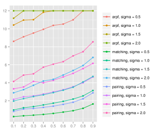
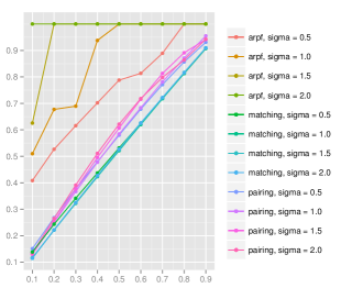
We define the cost of an $\alpha$SMC resampling step at time $n$ to be the average degree of the vertices in the forest corresponding to the $\alpha_{n-1}$ transition matrix chosen in $(\star)$ of Algorithm 1, which we denote $d_{n}^{N}$. For example, when $\alpha_{n-1}=Id$ the cost is $1$ and when $\alpha_{n-1}=\mathbf{1}_{1/N}$ the cost is $N$. We ran Algorithm 1 for $n=200$ iterations with various values of $\tau$ and $\sigma$ and $N=2^{12}=4096$ particles. One can think of the value of $N$ reported here as being a large multiple of $4096$ since, conceptually, one could imagine that the leaves in this experiment represent devices with a large number of particles. The tree $T_{0}$ used at each iteration always consisted of three levels with each node except the leaves having $2^{4}=16$ children, but the leaf/device indices were permuted at each iteration.

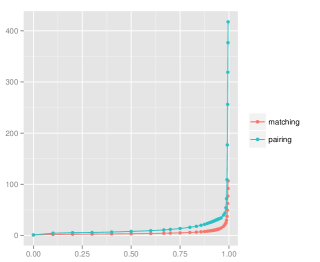
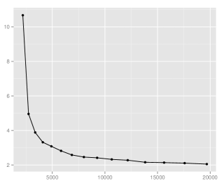
Figure 5 shows the behaviour of $\bar{d}=n^{-1}\sum_{p=1}^{n}d_{p}^{N}$ and $\overline{N^{\text{eff}}}=n^{-1}\sum_{p=1}^{n}N_{p}^{\text{eff}}$ as $\tau$ and $\sigma$ vary using the adaptive resampling particle filter (ARPF) of [12], and the two proposed strategies in Section 4.6, all instances of $\alpha$SMC. We can see that the ARPF is particularly expensive in terms of average degree, and has a higher average ESS than the rest. The pairing and matching strategies perform much better with the latter being less expensive and having an ESS much closer to the threshold. In all cases, increases in $\tau$ and $\sigma$ increase the cost of the algorithm, as one would expect. However, the shape of the curve in Figure 6a suggests that increasing $\tau$ beyond around $0.5$ rapidly becomes expensive. Indeed, the value $\tau=1$ corresponds to an average degree of $4096$ in this example for any of the methods, which is not shown, and is almost $10$ times larger than the corresponding cost for $\tau=224/225\approx 0.996$, the rightmost point shown. Figure 6b shows further that fixing $N\tau=2048$ but increasing $N$ has the effect of reducing the average degree to close to $2$ and suggests that optimizing, in terms of computational cost, the choice of $N$ and $\tau$ with a given target ESS $N\tau$ could involve choosing a large $N$ and a small $\tau$, depending on the relative cost of increasing $N$ compared to the cost in interactions.

(a)

(b)

Figure 5: Graphs of (a) $\log_{2}\bar{d}$ and (b) $\overline{N^{\text{eff}}}/N$ against $\tau$ for the various forest selection schemes and choices of $\sigma$.

(a) Plot of $\bar{d}$ against $\tau$ for $\sigma=1$.

(b) Plot of $\bar{d}$ against $N$ with $N\tau=2048$ for $\sigma=1$ using the matching strategy.

Figure 6: Dependence of $\bar{d}$ on $\tau$

5.2 Connection to existing sampling schemes

Resampling methods other than multinomial can be implemented using trees as well. In order to make this concrete, we assume that the tree is ordered, i.e., the children of each node written in sequence as $\chi_{1},\chi_{2},\ldots$. This imposes only the constraint that the labelling of children is consistent, and allows the specification of Algorithm 7, which implements Algorithm 4 with a single uniform random variable using the recycling method of [21, Section III.3.7]. Proposition 9 and the Remark that follows then imply that we can view this algorithm as a tree-based implementation of the inverse transform method for sampling from a categorical distribution.

Algorithm 7 Select a value in $\ell(\nu)$ given a $u\in[0,1]$

select$(\nu,u)$

1. If $\mathcal{C}(\nu)=\emptyset$, return the only element in $\ell(\nu)$.

2. Otherwise, let $\chi_{1},\ldots,\chi_{|\mathcal{C}(\nu)|}$ be the children of $\nu$ in order.

3. Set

   $$i\leftarrow\min\left\{k:\sum_{j=[k]}\mathcal{V}_{2}(\chi_{j})\geq u\sum_{j\in\left[\left|\mathcal{C}(\nu)\right|\right]}\mathcal{V}_{2}(\chi_{j})\right\}.$$

4. Return

   $$\mathtt{select}\left(\chi_{i},\frac{u\sum_{j\in\left[\left|\mathcal{C}(\nu)\right|\right]}\mathcal{V}_{2}(\chi_{j})-\sum_{j=[i-1]}\mathcal{V}_{2}(\chi_{j})}{\mathcal{V}_{2}(\chi_{i})}\right).$$

Proposition 9.

Assume that the tree is ordered such that for each node its children $(\chi_{i})$ have $j\in\ell(\chi_{i}),k\in\ell(\chi_{i+1})\implies j<k$. Calling Algorithm 7 with $(\nu,u)$ returns $\min\left\{k:\sum_{j\in\ell(\nu)\cap[k]}c^{j}\geq u\sum_{j\in\ell(\nu)}c^{j}\right\}$.

Remark.

The ordering specified above is w.r.t. the indices of particles and imposes no real constraint on how the tree is actually constructed, as long as a specific order is used in step 2 of Algorithm 7. If an alternative ordering is assumed in Proposition 9 the resulting returned value will still be deterministic and of the form given with a slight modification to account for this alternative ordering.

Multinomial resampling corresponds to sampling $N$ i.i.d. uniform random variables $u^{1},\ldots,u^{N}$ and calling select$(\nu,u^{i})$ for each $i\in[N]$, thereby providing $N$ i.i.d. draws from a categorical distribution. One can view other resampling methods as making dependent draws from a categorical distribution by the inverse transform method by using random variables $u^{1},\ldots,u^{N}$ that are not i.i.d. but for which the distribution of $u^{K}$, where $K$ is chosen uniformly at random from $[N]$, is uniform on $[0,1]$ [see, e.g., 22]. Therefore, to implement alternative resampling schemes, one again calls select$(\nu,u^{i})$ for each $i\in[N]$, but with $u^{1},\ldots,u^{N}$ are distributed in a dependent fashion as in [22]. The dependent $u^{i}$ can be interpreted as “trickling” down a tree whose leaves represent ancestor indices in a manner reminiscent of the approach in [23], which most closely resembles the systematic resampling scheme in [24].

5.3 Concluding Remarks

For ease of presentation, we have chosen to work with a particularly simple version of $\alpha$SMC, in which new samples are proposed using the HMM Markov kernel $f$. As noted in [11], the algorithm is easily generalized to accommodate other proposal kernels.

This paper, and the methodology of [11] more generally, naturally complements the contribution of [9]. In particular, the methods in the latter allow particles to be “reconstructed” on a device on the basis of only a small amount of communicated information, and could be used in tandem with the algorithms here in appropriate applications.

Both the approaches in Section 4.6 resemble in some ways greedy strategies for solving the classical Partition problem. It would be of interest to consider analogues of more sophisticated solutions to this problem such as those in [25] and [26]. More generally, it would be of interest to have quantitative theoretical results enabling the comparison of particular tree structures and partition selection schemes.

In practice, it may often be the case that devices are homogeneous, with the network connections between any two devices being of similar latency and bandwidth. In such situations, one will often create the structure of the tree at levels above the device and particle layers in a highly structured way. The use of a randomly generated tree may be beneficial, as suggested by the Random adaptation rule of [11, Section 5.4], which had however no hierarchy. A random permutation of the device nodes, in an otherwise constant tree was used in Section 5.1 for this reason.

Finally, this paper is concerned primarily with $\alpha$ matrices that are induced by disjoint unions of complete graphs, and hence have a particular structure. It would be of interest to explore similar results and methodology for more general $\alpha$ matrices.

Acknowledgements

We thank Dr. Kari Heine for assistance with the figures. The second author is supported in part by EPSRC grant EP/K023330/1.

Appendix A Proofs

Proof of Proposition 1.

It is straightforward to show that if $a\in\mathbb{A}_{V}$ then $\sum_{i}a^{ij}=\sum_{i\in V}a^{ij}=\mathbb{I}(j\in V)$. Therefore,

$$N^{{\rm eff}}(a,c) = \frac{\left(\sum_{i}\sum_{j}a^{ij}c^{j}\right)^{2}}{\sum_{i}\left(\sum_{j}a^{ij}c^{j}\right)^{2}}=\frac{\left(\sum_{i\in V}\sum_{j\in V}a^{ij}c^{j}\right)^{2}}{\sum_{i\in V}\left(\sum_{j\in V}a^{ij}c^{j}\right)^{2}}$$

$$= \frac{\left(\sum_{j\in V}c^{j}\right)^{2}}{\sum_{i\in V}\left(\sum_{j\in V}a^{ij}c^{j}\right)^{2}}.$$

We define $x_{1}:=\sum_{j\in V}c^{j}$, $x_{2}:=\sum_{j\in V^{\prime}}c^{j}$, $y_{1}:=\sum_{i\in V}\left(\sum_{j\in V}a^{ij}c^{j}\right)^{2}$, $y_{2}:=\sum_{i\in V^{\prime}}\left(\sum_{j\in V^{\prime}}\left(a^{\prime}\right)^{ij}c^{j}\right)^{2}$ and $\tilde{y}_{2}:=\sum_{i\in V^{\prime}}\left(\sum_{j\in V^{\prime}}\left(\tilde{a}^{\prime}\right)^{ij}c^{j}\right)^{2}$. This allows us to write $N^{{\rm eff}}\left(a,c\right)=x_{1}^{2}/y_{1}$, $N^{{\rm eff}}\left(a^{\prime},c\right)=x_{2}^{2}/y_{2}$ and $N^{{\rm eff}}\left(\tilde{a}^{\prime},c\right)=x_{2}^{2}/\tilde{y}_{2}$, and since $V\cap V^{\prime}=\emptyset$, $N^{{\rm eff}}\left(a+a^{\prime},c\right)=(x_{1}+x_{2})^{2}/(y_{1}+y_{2})$ and $N^{{\rm eff}}\left(a+\tilde{a}^{\prime},c\right)=(x_{1}+x_{2})^{2}/(y_{1}+\tilde{y}_{2})$.

1. The lower bound holds because

$$\left(\sum_{i}\sum_{j}a^{ij}c^{j}\right)^{2} = \sum_{i,k}\left(\sum_{j}a^{ij}c^{j}\right)\left(\sum_{j}a^{kj}c^{j}\right)$$

$$\geq \sum_{i}\left(\sum_{j}a^{ij}c^{j}\right)^{2},$$

so $N^{{\rm eff}}(a,c)\geq 1$. The upper bound holds because, using Jensen’s inequality,

$$\left(\sum_{i}\sum_{j}a^{ij}c^{j}\right)^{2} = |V|^{2}\left(\sum_{i\in V}|V|^{-1}\sum_{j\in V}a^{ij}c^{j}\right)^{2}$$

$$\leq |V|^{2}\sum_{i\in V}|V|^{-1}\left(\sum_{j\in V}a^{ij}c^{j}\right)^{2}$$

$$= |V|\sum_{i\in V}\left(\sum_{j\in V}a^{ij}c^{j}\right)^{2},$$

so $N^{{\rm eff}}(a,c)\leq|V|$. The upper bound is attained when $a^{ij}=|V|^{-1}\mathbb{I}\left(i,j\in V\right)$ since then

$$\sum_{i\in V}\left(\sum_{j\in V}a^{ij}c^{j}\right)^{2} = \sum_{i\in V}\left(\sum_{j\in V}|V|^{-1}c^{j}\right)^{2}$$

$$= |V|^{-1}\left(\sum_{j\in V}c^{j}\right)^{2}.$$

2. The result follows from

$$N^{{\rm eff}}\left(a,c\right)+N^{{\rm eff}}\left(a^{\prime},c\right)-N^{{\rm eff}}\left(a+a^{\prime},c\right)$$

$$= \frac{x_{1}^{2}}{y_{1}}+\frac{x_{2}^{2}}{y_{2}}-\frac{(x_{1}+x_{2})^{2}}{y_{1}+y_{2}}$$

$$= x_{1}^{2}\left\{\frac{y_{2}}{y_{1}(y_{1}+y_{2})}\right\}+x_{2}^{2}\left\{\frac{y_{1}}{y_{2}(y_{1}+y_{2})}\right\}-\frac{2x_{1}x_{2}}{y_{1}+y_{2}}$$

$$= \frac{y_{1}y_{2}}{y_{1}+y_{2}}\left(\frac{x_{1}}{y_{1}}-\frac{x_{2}}{y_{2}}\right)^{2}\geq 0,$$

with equality only when $\frac{x_{1}}{y_{1}}=\frac{x_{2}}{y_{2}}$, corresponding to $\frac{\sum_{j\in V}c^{j}}{N^{{\rm eff}}(a,c)}=\frac{\sum_{j\in V^{\prime}}c^{j}}{N^{{\rm eff}}(a^{\prime},c)}$.

3. Since $N^{{\rm eff}}(a^{\prime},c)\leq N^{{\rm eff}}(\tilde{a}^{\prime},c)\implies y_{2}\geq\tilde{y}_{2}$,

$$N^{{\rm eff}}(a+\tilde{a}^{\prime},c)-N^{{\rm eff}}(a+a^{\prime},c)$$

$$=\frac{\left(x_{1}+x_{2}\right)^{2}}{y_{1}+\tilde{y}_{2}}-\frac{\left(x_{1}+x_{2}\right)^{2}}{y_{1}+y_{2}}\geq 0,$$

with equality only when $y_{2}=\tilde{y}_{2}$, corresponding to $N^{{\rm eff}}(a^{\prime},c)\leq N^{{\rm eff}}(\tilde{a}^{\prime},c)$.

4. We have

$$N^{{\rm eff}}\left(a_{1}+a_{2},c\right)$$

$$=\frac{(x_{1}+x_{2})^{2}}{y_{1}+y_{2}}$$

$$=\frac{x_{1}^{2}}{y_{1}}\cdot\frac{y_{1}}{y_{1}+y_{2}}+\frac{2x_{1}x_{2}}{y_{1}+y_{2}}+\frac{x_{2}^{2}}{y_{2}}\cdot\frac{y_{2}}{y_{1}+y_{2}}$$

$$\geq\min_{i}\left\{\frac{x_{i}^{2}}{y_{i}}\right\}=\min\left\{N^{{\rm eff}}\left(a,c\right),N^{{\rm eff}}\left(a^{\prime},c\right)\right\}.$$

∎

Proof of Proposition 2.

We prove the result for $\mathbb{G}$ since the result for $\mathbb{A}_{\mathbb{G}}$ then follows. Let $V\subseteq[N]$ and consider $G_{1}=(V,E_{1})$, $G_{2}=(V,E_{2})$ and $G_{3}=(V,E_{3})$. It suffices to check that $\preceq$ is reflexive ($G_{1}\preceq G_{1})$, antisymmetric ($G_{1}\preceq G_{2}$ and $G_{2}\preceq G_{1}$ implies $G_{1}=G_{2}$) and transitive ($G_{1}\preceq G_{2}$ and $G_{2}\preceq G_{3}$ implies $G_{1}\preceq G_{3}$). Since $E_{1}\subseteq E_{1}$, it follows that $G_{1}\preceq G_{1}$. When $G_{1}\preceq G_{2}$ and $G_{2}\preceq G_{1}$, this implies $E_{1}\subseteq E_{2}$ and $E_{2}\subseteq E_{1}$ and it follows that $E_{1}=E_{2}$ and so $G_{1}=G_{2}$. Finally, $G_{1}\preceq G_{2}$ and $G_{2}\preceq G_{3}$ implies that $E_{1}\subseteq E_{2}$ and $E_{2}\subseteq E_{3}$ and so $E_{1}\subseteq E_{3}$ and therefore $G_{1}\preceq G_{3}$. ∎

Proof of Proposition 3.

Since $a\preceq\tilde{a}$ we have that $a,\tilde{a}\in\mathbb{A}_{\mathbb{G}}\cap\mathbb{A}_{V}$ for some $V\subseteq[N]$. Therefore, for some $K,\tilde{K}\in[N]$ we can write $a=\sum_{k\in[K]}\phi(\kappa(V_{k}))$ and $\tilde{a}=\sum_{\tilde{k}\in[\tilde{K}]}\phi(\kappa(\tilde{V}_{\tilde{k}}))$ where each $V_{k}$ and $\tilde{V}_{\tilde{k}}$ are subsets of $V$. Since $a\preceq\tilde{a}$, for each $k\in[K]$ there exists $\tilde{k}\in[\tilde{K}]$ such that $V_{k}\subseteq\tilde{V}_{\tilde{k}}$. We now define a sequence, with $a_{0}=a$, and for $i\in[\tilde{K}]$

$$a_{i}:=a_{i-1}+\phi(\kappa(\tilde{V}_{i}))-\sum_{k\in[K],V_{k}\cap\tilde{V}_{i}\neq\emptyset}\phi(\kappa(V_{k})),$$

and note that $a_{\tilde{K}}=\tilde{a}$. Now for each $i\in[\tilde{K}]$, $a_{i}\in\mathbb{A}_{\mathbb{G}}\cap\mathbb{A}_{V}$ and letting $\check{V}_{i}:=\bigcup_{j=1}^{i}\tilde{V}_{j}$ and

$$b_{i}:=\sum_{k\in[K],V_{k}\cap\check{V}_{i}=\emptyset}\phi(\kappa(V_{k}))+\sum_{j=1}^{i-1}\phi(\kappa(\tilde{V}_{j})),$$

we can write $a_{i-1}=b_{i}+\sum_{k\in[K],V_{k}\cap\tilde{V}_{i}\neq\emptyset}\phi(\kappa(V_{k}))$ and $a_{i}=b_{i}+\phi(\kappa(\tilde{V}_{i}))$. From the first part of Proposition 1 we have that $N^{{\rm eff}}\left(\sum_{k\in[K],V_{k}\cap\tilde{V}_{i}\neq\emptyset}\phi(\kappa(V_{k})),c\right)\leq\left|\tilde{V}_{i}\right|=\phi(\kappa(\tilde{V}_{i}))$ and so by the monotonicity property in Proposition 1 we have $N^{{\rm eff}}(a_{i-1},c)\leq N^{{\rm eff}}(a_{i},c)$ for each $i\in[\tilde{K}]$. It follows that $N^{{\rm eff}}(a,c)\leq N^{{\rm eff}}(\tilde{a},c)$. ∎

Proof of Proposition 4.

The first inequality follows from Proposition 3 since $a\preceq\tilde{a}$. For the second inequality, assume that $\min_{k}\left|V_{k}\right|^{-1}N^{{\rm eff}}(a_{k},c)\geq D$. This implies that for any $k\in[K]$,

$$\sum_{i\in V_{k}}\left(\sum_{j\in V_{k}}a_{k}^{ij}c^{j}\right)^{2}\leq\frac{1}{D|V_{k}|}\left(\sum_{j\in V_{k}}c^{j}\right)^{2}.$$

Therefore

$$N^{{\rm eff}}\left(a,c\right) = \frac{\left(\sum_{k\in[K]}\sum_{j\in V_{k}}c^{j}\right)^{2}}{\sum_{k\in[K]}\sum_{i\in V_{k}}\left(\sum_{j\in V_{k}}a_{k}^{ij}c^{j}\right)^{2}}$$

$$\geq D\frac{\left(\sum_{k\in[K]}\sum_{j\in V_{k}}c^{j}\right)^{2}}{\sum_{k\in[K]}|V_{k}|^{-1}\left(\sum_{j\in V_{k}}c^{j}\right)^{2}}$$

$$= DN^{{\rm eff}}\left(\tilde{a},c\right).$$

∎

Proof of Proposition 5.

The proof is by induction. Note that $\tau\in[0,1]$. If $|V|=1$ then $|P|=1$ and $N_{c}^{{\rm eff}}(P)=1$, so the claim is true. Now assume that the claim holds true for all $V$ with $|V|\in[s-1]$, $s\in\mathbb{N}$, and consider the case where $|V|=s$. First, note that if $P=\{V\}$ then $N^{{\rm eff}}(P,c)=|V|$ by Proposition 1 and so if $|P|=1$ the claim is true. It remains to check that if $|P|>1$ then $a=\sum_{k\in[K]}a_{k}$ satisfies the claim, where $a_{k}={\tt choose.a}(V_{k},\tau/\rho(P,c))$. By the induction hypothesis, for each $k\in[K]$, $N^{{\rm eff}}(a_{k},c)/\left|V_{k}\right|\geq\tau/\rho(P,c)$ since $|V_{k}|\in[s-1]$ and $\tau/\rho(P,c)\in[0,1]$. Then by Proposition 4, with $\tilde{a}=\sum_{k\in[K]}\phi(\kappa(V_{k}))$,

$$N^{{\rm eff}}\left(a,c\right) \geq \min_{k}\left\{\frac{N^{{\rm eff}}(a_{k},c)}{|V_{k}|}\right\}N^{{\rm eff}}\left(\tilde{a},c\right)$$

$$\geq \frac{\tau}{\rho(P,c)}\rho(P,c)\left|V\right|=\tau\left|V\right|,$$

and we conclude. ∎

Proof of Proposition 6.

Let $s_{\nu}(j)$ denote the probability that Algorithm 4 returns $j\in\ell(\nu)$. Given $j\in\ell(\nu)$, let $\nu^{1}$ be the parent of $\nu_{j}$, $\nu^{2}$ be the parent of $\nu^{1}$, etc., until $\nu^{m}=\nu$ is the parent of $\nu^{m-1}$. Then

$$s_{\nu}(j) = \frac{c^{j}}{\sum_{k\in\ell(\nu^{1})}c^{k}}\prod_{i\in[m-1]}\frac{\sum_{k\in\ell(\nu^{i})}c^{k}}{\sum_{k\in\ell(\nu^{i+1})}c^{k}},$$

$$= \frac{c^{j}}{\sum_{k\in\ell(\nu)}c^{k}}=p_{\mathcal{S}(\nu)}(j).$$

∎

Proof of Proposition 7.

We define $x_{i}:=\sum_{j\in V_{i}}c^{j}$ for $i\in[2M]$ and it suffices to show that $P^{\prime}$ minimizes the denominator of $\rho(\cdot,c)$,

$$r(P^{\prime},c):=\left(2\left|V_{1}\right|\right)^{-1}\sum_{S\in P^{\prime}}\left(\sum_{i\in S}x_{i}\right)^{2},$$

since each element of any pairing of $P$ is of size $2\left|V_{1}\right|$. We first prove that $V_{1}\cup V_{2M}$ is a member of at least one pairing of $P$ that minimizes $r(\cdot,c)$. Indeed, assume that a pairing $\check{P}$ that minimizes $r(\cdot,c)$ is given. We will show that a pairing $\check{P}^{\prime}$ containing $V_{1}\cup V_{2M}$ exists for which $r(\check{P}^{\prime},c)\leq r(\check{P},c)$. Let $V_{1}\cup V_{j}$ and $V_{k}\cup V_{2M}$ be elements of $\check{P}$. We define $\check{P}^{\prime}=\check{P}\setminus\{V_{1}\cup V_{j},V_{k}\cup V_{2M}\}\cup\{V_{1}\cup V_{2M},V_{k}\cup V_{j}\}$. Then

$$2\left|V_{1}\right|\left(r(\check{P},c)-r(\check{P}^{\prime},c)\right)$$

$$= \sum_{S\in\check{P}}\left(\sum_{i\in S}x_{i}\right)^{2}-\sum_{S\in\check{P}^{\prime}}\left(\sum_{i\in S}x_{i}\right)^{2}$$

$$= \left(x_{1}+x_{j}\right)^{2}+\left(x_{k}+x_{2M}\right)^{2}$$

$$-\left(x_{1}+x_{2M}\right)^{2}-\left(x_{k}+x_{j}\right)^{2}$$

$$= 2x_{1}x_{j}+2x_{k}x_{2M}-2x_{1}x_{2M}-2x_{k}x_{j}$$

$$= 2x_{k}(x_{2M}-x_{j})-2x_{1}(x_{2M}-x_{j})$$

$$= 2(x_{k}-x_{1})(x_{2M}-x_{j})\geq 0,$$

since $x_{1}$ and $x_{2M}$ are the minimal and maximal values of $\{x_{i}:i\in[2M]\}$, respectively.

Now, let $\check{P}^{\prime}$ be a pairing of $P$ and $S=V_{1}\cup V_{2M}\in\check{P}^{\prime}$. Then $r(\check{P}^{\prime},c)=r(\{S\},c)+r(\check{P}^{\prime}\setminus\{S\},c)$ and so it follows that if $\check{P}^{\prime}$ minimizes $r(\cdot,c)$ then $\check{P}^{\prime}\setminus\{S\}$ is a pairing of $P\setminus\left\{V_{1},V_{2M}\right\}$ that minimizes $r(\cdot,c)$. It then follows that at least one pairing $\check{P}^{\prime}$ of $P$ that minimizes $r(\cdot,c)$ is the union of $V_{1}\cup V_{2M}$ and a pairing of $P\setminus\left\{V_{2M},V_{1}\right\}$ that minimizes $r(\cdot,c)$. But then the argument above shows that $V_{2}\cup V_{2M-1}$ is a valid element of such a minimizing pairing. Continuing, we obtain that $P^{\prime}$ is a pairing of $P$ that minimizes $r(\cdot,c)$ and we conclude. ∎

Proof of Proposition 8.

From (12) we can write $\rho(P{}_{k,l},c)=\rho(P,c)\frac{r(P,c)}{r(P_{k,l},c)}$ where $r(P,c):=\sum_{S\in P}|S|\left(|S|^{-1}\sum_{j\in S}c^{j}\right)^{2}$. It suffices therefore to find $k,l\in[K]$ minimizing $r(P_{k,l},c)$. Letting $m_{i}=\left|V_{i}\right|$ and $x_{i}=\sum_{j\in V_{i}}c^{j}$, we can write

$$r(P_{k,l},c) = r(P,c)-\frac{x_{k}^{2}}{m_{k}}-\frac{x_{l}^{2}}{m_{l}}+\frac{\left(x_{k}+x_{l}\right)^{2}}{m_{k}+m_{l}}$$

$$= r(P,c)-\frac{m_{k}m_{l}}{m_{k}+m_{l}}\left(\frac{x_{k}}{m_{k}}-\frac{x_{l}}{m_{l}}\right)^{2},$$

the equality following along the same lines as the proof of the second part of Proposition 1, and we conclude. ∎

Proof of Proposition 9.

Let $\chi_{\nu}:=\left(\chi_{\nu,1},\ldots,\chi_{\nu,K}\right)$ be the ordered children of $\nu$, where $|\mathcal{C}(\nu)|=K$. To alleviate notation, we define $c(\chi_{\nu,k}):=\sum_{j\in\ell(\chi_{\nu,k})}c^{j}$, $k_{\nu}(u):=\min\left\{k:\sum_{j\in[k]}c(\chi_{\nu,j})\geq u\sum_{j\in\ell(\nu)}c^{j}\right\}$ and $s_{\nu}(k):=\sum_{j\in[k]}c(\chi_{\nu,j})$. Algorithm 7 with input $(\nu,u)$ returns $f_{\nu}(u)$, where

$$f_{\nu}(u):=\begin{cases}\min\ell(\nu)&\left|\ell(\nu)\right|=1,\\ f_{\chi_{\nu,k_{\nu}(u)}}\left(\frac{u\sum_{j\in\ell(\nu)}c^{j}-s_{\nu}(k_{\nu}(u)-1)}{c(\chi_{\nu,k_{\nu}(u)})}\right)&\text{otherwise.}\end{cases}$$

Now we prove by induction that $f_{\nu}(u)=\min\left\{k:\sum_{j\in\ell(\nu)\cap[k]}c^{j}\geq u\sum_{j\in\ell(\nu)}c^{j}\right\}$. If $|\ell(\nu)|=1$, the claim is trivially true. Now assume the claim is true for $\{\nu:|\ell(\nu)|\in[p-1]\}$ and consider $\nu$ with $|\ell(\nu)|=p>1$. We have

$$f_{\nu}(u)=f_{\chi_{\nu,k_{\nu}(u)}}\left(\frac{u\sum_{j\in\ell(\nu)}c^{j}-s_{\nu}(k_{\nu}(u)-1)}{c(\chi_{\nu,k_{\nu}(u)})}\right)$$

and we can apply the induction hypothesis since $|\ell(\chi_{\nu,k_{\nu}(u)})|\in[p-1]$. Therefore, letting $y:=u\sum_{j\in\ell(\nu)}c^{j}-s_{\nu}(k_{\nu}(u)-1)$, and $x:=\chi_{\nu,k_{\nu}(u)}$we can write $f_{\nu}(u)$ as

$$\min\left\{k:\sum_{j\in\ell(x)\cap[k]}c^{j}\geq\frac{y}{c(x)}\sum_{j\in\ell(x)}c^{j}\right\}$$

$$= \min\left\{k:\sum_{j\in\ell(x)\cap[k]}c^{j}\geq u\sum_{j\in\ell(\nu)}c^{j}-s_{\nu}(k_{\nu}(u)-1)\right\}$$

$$= \min\left\{k:\sum_{j\in\ell(\nu)\cap[k]}c^{j}\geq u\sum_{j\in\ell(\nu)}c^{j}\right\},$$

and we conclude. ∎

References

- Doucet et al. [2000] A. Doucet, S. Godsill, and C. Andrieu. On sequential Monte Carlo sampling methods for Bayesian filtering. Stat. Comput., 10(3):197–208, 2000.
- Doucet and Johansen [2008] A. Doucet and A. M. Johansen. A tutorial on particle filtering and smoothing: Fifteen years later. In D. Crisan and B. Rozovsky, editors, Handbook of Nonlinear Filtering. Oxford University Press, 2008.
- Chopin [2002] N. Chopin. A sequential particle filter method for static models. Biometrika, 89(3):539–552, 2002.
- Del Moral et al. [2006] P. Del Moral, A. Doucet, and A. Jasra. Sequential Monte Carlo samplers. J. R. Stat. Soc. Ser. B Stat. Methodol., 68(3):411–436, 2006.
- Chopin et al. [2013] N. Chopin, P. E. Jacob, and O. Papaspiliopoulos. SMC2: an efficient algorithm for sequential analysis of state space models. J. R. Stat. Soc. Ser. B Stat. Methodol., 75(3):397–426, 2013.
- Suchard and Rambaut [2009] M. A. Suchard and A. Rambaut. Many-core algorithms for statistical phylogenetics. Bioinformatics, 25(11):1370–1376, 2009.
- Lee et al. [2010] A. Lee, C. Yau, M. B. Giles, A. Doucet, and C. C. Holmes. On the utility of graphics cards to perform massively parallel simulation of advanced Monte Carlo methods. J. Comput. Graph. Statist., 19(4):769–789, 2010.
- Bolić et al. [2005] M. Bolić, P. M. Djurić, and S. Hong. Resampling algorithms and architectures for distributed particle filters. IEEE Trans. Signal Process., 53(7):2442–2450, 2005.
- Jun et al. [2012] S.-H. Jun, L. Wang, and A. Bouchard-Côté. Entangled monte carlo. In Advances in Neural Information Processing Systems, pages 2726–2734, 2012.
- [10] C. Vergé, C. Dubarry, P. Del Moral, and E. Moulines. On parallel implementation of sequential Monte Carlo methods: the island particle model. Stat. and Comput. To appear.
- Whiteley et al. [2013] N. Whiteley, A. Lee, and K. Heine. On the role of interaction in sequential Monte Carlo algorithms. arXiv preprint 1309.2918, 2013.
- Liu and Chen [1995] J. S. Liu and R. Chen. Blind deconvolution via sequential imputations. J. Amer. Statist. Assoc., 90(430):567–576, 1995.
- Del Moral and Guionnet [2001] P. Del Moral and A. Guionnet. On the stability of interacting processes with applications to filtering and genetic algorithms. Ann. Inst. Henri Poincaré Probab. Stat., 37(2):155–194, 2001.
- Cérou et al. [2011] F. Cérou, P. Del Moral, and A. Guyader. A nonasymptotic variance theorem for unnormalized Feynman Kac particle models. Ann. Inst. Henri Poincaré Probab. Stat., 47(3):629–649, 2011.
- Whiteley and Lee [2014] N. Whiteley and A. Lee. Twisted particle filters. Ann. Statist., 42(1):115–141, 2014.
- Whiteley [2013] N. Whiteley. Stability properties of some particle filters. Ann. Appl. Probab., 23(6):2500–2537, 2013.
- Knuth [1997] D. E. Knuth. The Art of Computer Programming, volume 1. Addison-Wes, 3rd edition, 1997.
- Hillis and Steele Jr [1986] W. D. Hillis and G. L. Steele Jr. Data parallel algorithms. Communications of the ACM, 29(12):1170–1183, 1986.
- Isard et al. [2007] M. Isard, M. Budiu, Y. Yu, A. Birrell, and D. Fetterly. Dryad: distributed data-parallel programs from sequential building blocks. ACM SIGOPS Operating Systems Review, 41(3):59–72, 2007.
- Mertens [2006] S. Mertens. The easiest hard problem: number partitioning. In A. Percus, G. Istrate, and C. Moore, editors, Computational Complexity and Statistical Physics, pages 125–139. Oxford University Press, 2006.
- Devroye [1986] L. Devroye. Non-uniform random variate generation. Springer Verlag, 1986.
- Douc et al. [2005] R. Douc, O. Cappé, and E. Moulines. Comparison of resampling schemes for particle filtering. In Proceedings of the 4th International Symposium on Image and Signal Processing and Analysis, pages 64–69, 2005.
- Crisan and Lyons [2002] D. Crisan and T. Lyons. Minimal entropy approximations and optimal algorithms for the filtering problem. Monte Carlo methods and applications, 8(4):343–356, 2002.
- Kitagawa [1996] G. Kitagawa. Monte Carlo filter and smoother for non-Gaussian nonlinear state space models. J. Comput. Graph. Statist., 5(1):1–25, 1996.
- Karmarkar and Karp [1982] N. Karmarkar and R. M. Karp. The differencing method of set partitioning. Technical report, University of California, Berkeley, 1982.
- Korf [1995] R. E. Korf. From approximate to optimal solutions: A case study of number partitioning. In Proceedings of the 14th international joint conference on Artificial intelligence, pages 266–272, 1995.