Effective spin-1/2 exchange interactions in Tb₂Ti₂O₇

Abstract

We derive an effective spin-1/2 exchange model for non-Kramers Tb³⁺ states in the pyrochlore Tb₂Ti₂O₇. The four anisotropic nearest-neighbour exchange constants, as well as next-neighbour exchange constants are derived for the effective model. This work goes beyond the independent tetrahedra model by considering all nearest-neighbour exchange paths on the pyrochlore lattice. Estimates of the exchange constants reveal that Tb₂Ti₂O₇ is described by a quantum spin ice Hamiltonian.

I Introduction

The rare-earth pyrochlore magnets, with chemical formula R₂Ti₂O₇, exhibit a variety of low-temperature phenomena, from magnetic ordering in Er₂Ti₂O₇ [champion2003, ], to spin ice states in Ho₂Ti₂O₇ [harris1997, ] and Dy₂Ti₂O₇ [ramirez1999, ], and possible spin liquid behaviour in Tb₂Ti₂O₇ [gardner2001, ]. In each case, the magnetic properties are due to the magnetic moments of the rare earth ions, which are proportional to $J$, the total angular momentum of the ion, and to interactions between them. In spite of rather large values of $J$ derived from Hund’s rules, the rare-earth pyrochlores are essentially quantum magnets: a strong crystal electric field (CEF) lowers the $2J+1$-fold degeneracy of the rare earth ions into singlets and doublets, with rather large energy differences between the levels. In many cases, the CEF ground state is a doublet, which is treated as a basic two-level quantum mechanical system.

Recently, there has been a great deal of effort to describe these various rare earth pyrochlores within the same phenomenological model, the spin-1/2 nearest-neighbour exchange interaction. This modeling process is straightforward for materials such as Er₂Ti₂O₇ and Yb₂Ti₂O₇, whose CEF ground state doublets are in fact spinors. However, Tb₂Ti₂O₇ has proven to be especially difficult to model, for two reasons. First, the CEF ground state doublet of Tb₂Ti₂O₇ is not a spinor. Second, Tb₂Ti₂O₇ is complicated by the presence of a low-lying CEF excited state just 17.9 K above the ground state, which tends to mix into the ground state because of the exchange interaction.

The rare earth ions in pyrochlore crystals are located at the 16d Wyckoff position of the space group $Fd\bar{3}m$. There are four 16d sites in the primitive unit cell, located on the vertices of a tetrahedron. The local site symmetry (CEF symmetry) is $D_{3d}$. The 3-fold ($C_{3}$) axes point in different directions for the different sites: $[111]$, $[1\bar{1}\bar{1}]$, $[\bar{1}1\bar{1}]$ and $[1\bar{1}\bar{1}]$ for sites #1, 2, 3 and 4 respectively. These directions define a local $z$-axis for each site on a tetrahedron. For non-Kramers ions (such as Tb³⁺ or Ho³⁺), the CEF states are singlets or doublets belonging to the $A_{1}$, $A_{2}$ or $E$ representations of $D_{3}$. For Kramers ions (such as Er³⁺, Yb³⁺ or Dy³⁺), the CEF states are doublets belonging to either the $\Gamma_{4}$ or $\Gamma_{5}$ representations of $D_{3}^{\prime}$, the double group of $D_{3}$. The CEF ground states for Er³⁺ in Er₂Ti₂O₇ and Yb³⁺ in Yb₂Ti₂O₇ belong to $\Gamma_{4}$, which is isomorphic to spin-1/2. Therefore CEF ground state doublets of Er³⁺ and Yb³⁺ can be easily mapped to a spin-1/2 spinor by an appropriate renormalisation of the matrix elements for the operators $J_{z}$ and $J_{\pm}$. Here we are concerned with finding a map between the non-Kramers ($E$) doublet and a spin-1/2 ($\Gamma_{4}$) doublet. Because these two kinds of doublets transform differently under rotations, such a map must be constructed with care. In fact, a symmetry-preserving map exists if these doublets are considered in groups of 4 (the four vertices of a tetrahedron in the pyrochlore lattice).

In the following section, we describe the CEF ground state of Tb₂Ti₂O₇, and the map between Tb₂Ti₂O₇ and spin-1/2 single tetrahedron states is defined. The exchange interaction is treated in Section III, for the general case, the spin-1/2 case, and for Tb₂Ti₂O₇. A map between spin-1/2 and Tb₂Ti₂O₇ exchange models is given in Section IV. The magnetisation is discussed in Section V. Section VI contains concluding remarks.

II Quantum mechanical states for Tb₂Ti₂O₇

II.1 CEF ground state for Tb³⁺ in Tb₂Ti₂O₇

The CEF Hamiltonian for the rare earth sites in R₂Ti₂O₇ is given by

$$H_{\rm{CEF}}=B^{0}_{2}O^{0}_{2}+B^{0}_{4}O^{0}_{4}+B^{3}_{4}O^{3}_{4}+B^{0}_{6}O^{0}_{6}+B^{3}_{6}O^{3}_{6}+B^{6}_{6}O^{6}_{6}$$ (1)

where $O^{i}_{j}$ are Stevens operators, $j$-th order polynomials of the operator $\vec{J}$, the total angular momentum. $B^{i}_{j}$ are constants determined experimentally. There have been several determinations of $B^{i}_{j}$ for Tb₂Ti₂O₇; allgingras2000 ; mirebeau2007 ; bertin2012 but the most recentzhang2014 are consistent with each other. The differences in these constants do not affect the symmetries of the CEF states, but they are eventually reflected in the exchange constants (see Section V).

According to Hund’s rules, the total angular momentum of the Tb³⁺ ion is $J=6$. The CEF lifts the 13-fold degeneracy into singlets and doublets. The CEF ground state of Tb³⁺ in Tb₂Ti₂O₇ is a doublet,bertin2012

$$|\pm\rangle=\pm 0.263|\pm 5\rangle-0.131|\pm 2\rangle\mp 0.128|\mp 1\rangle-0.947|\mp 4\rangle$$ (2)

where the quantisation axis points along the $C_{3}$ axis, which points in a different direction at each site. The quantisation axis defines a local $z$-axis. In this way, a different set of local axes is defined for each site on a tetrahedron (see Appendix A for a detailed description). The matrix elements for the operators $J_{\pm}\equiv J_{x}\pm iJ_{y}$ within the $|\pm\rangle$ doublet are zero, while

$$j_{1}\equiv\langle+|J_{z}|+\rangle=-3.21.$$ (3)

Here $x,y,z$ subscripts are used to denote local axes, while superscripts will be used to denote global axes.

II.2 The first excited CEF state for Tb³⁺ in Tb₂Ti₂O₇

In Tb₂Ti₂O₇, the first excited CEF state (also a doublet) lies only $\Delta=17.90$ K above the ground state. Therefore, as was recognised long ago,aleksandrov1981 ; aleksandrov1985 there is a significant admixture of this excited state to the lowest energy states. However, the symmetry of the lowest energy states cannot be affected by this admixture.

The first excited CEF state isbertin2012

$$|\uparrow/\downarrow\rangle=\mp 0.923|\pm 5\rangle+0.251|\pm 2\rangle\mp 0.082|\mp 1\rangle-0.280|\mp 4\rangle$$

The matrix element for $J_{z}$ within this doublet is

$$j_{2}\equiv\langle\uparrow|J_{z}|\uparrow\rangle=4.05,$$ (4)

and the matrix elements for $J_{\pm}$ are again zero. The mixing of the first CEF excited state to the ground state will depend on the matrix elements

$$j_{3}\equiv\langle\uparrow|J_{z}|+\rangle=-2.37$$ (5)

and

$$t\equiv\langle\uparrow|J_{+}|-\rangle=4.72.$$ (6)

II.3 Map between states

With four sites per tetrahedron, there are sixteen Tb₂Ti₂O₇ tetrahedron states of the form $|\pm\pm\pm\pm\rangle_{\rm Tb}\equiv|\pm\rangle_{1}\otimes|\pm\rangle_{2}\otimes|\pm\rangle_{3}\otimes|\pm\rangle_{4}$, where $|\pm\rangle_{i}$ is a non-Kramers doublet on the $i$th site. In a similar fashion, we can also define sixteen spin-1/2 tetrahedron states, which will be denoted as $|\pm\pm\pm\pm\rangle_{\frac{1}{2}}$. Each of these kets represents a classical state where each spin can be visualised as pointing into or out of the tetrahedron. There are two anti-ferromagnetic states, $|----\rangle$ and $|++++\rangle$, with all four spins pointing into ($-$) or out of $(+$) the tetrahedron (“all-in/all-out” states), while the six states of the form $|++--\rangle$ are ferromagnetic, with two spins pointing in and two spins pointing out of the tetrahedron (“2-in-2-out” spin ice states). In addition, there are eight “3-in-1-out/1-in-3-out” states.

The symmetry group of a tetrahedron in the pyrochlore lattice is $T_{d}$, with representations $A_{1}$, $A_{2}$, $E$, $T_{1}$ and $T_{2}$. Both the Tb₂Ti₂O₇  and the spin-1/2 tetrahedron states can be used as basis functions to generate a (reducible) representation of $T_{d}$. In both cases, in spite of different transformation properties of the individual site states, the decomposition is $A_{1}\oplus 3E\oplus 2T_{1}\oplus T_{2}$. This finding allows us to define a map between the Tb₂Ti₂O₇ (non-Kramers) tetrahedron states and spin-1/2 tetrahedron states. The map between the Tb₂Ti₂O₇ and spin-1/2 tetrahedron basis states is

$$|\pm\pm\pm\pm\rangle_{{\rm Tb}}\sim(-1)^{\eta}{\cal K}\left|\pm\pm\pm\pm\right\rangle_{\frac{1}{2}}$$ (7)

where ${\cal K}$ stands for time reversal (represented in the standard way as $-i\sigma_{y}{\cal K}_{0}$, where ${\cal K}_{0}$ is complex conjugation) and the exponent $\eta=0$ for the 2-in-2-out states and the 3-in-1-out spin-1/2 states (but not the 1-in-3-out states); $\eta=1$ otherwise. The phase $(-1)^{\eta}$ is a reflection of the non-triviality of the map.

It is worth noting that the tetrahedron states formed from the third kind of doublet (belonging to the $\Gamma_{5}$ representation of $D_{3}^{\prime}$) generate a representation with decomposition $3A_{1}\oplus 2A_{2}\oplus E\oplus 2T_{1}\oplus T_{2}$. Therefore there is no map between $\Gamma_{5}$ tetrahedron states and spin-1/2 tetrahedron states that is generally valid. The CEF ground state of Dy³⁺ in Dy₂Ti₂O₇ belongs to this case.

III The exchange interaction

III.1 Nearest neighbour exchange interaction: general

The exchange interaction is a phenomenological model that describes the energy dependence of different relative orientations of neighbouring magnetic moments. The general form of the exchange Hamiltonian is governed by the symmetry of the crystal. In a highly symmetric crystal, the number of free parameters of the Hamiltonian is small.

The most general form of the of the nearest neighbour exchange interaction on the pyrochlore lattice iscurnoe2008

$$H_{\rm ex}={\cal J}_{1}X_{1}+{\cal J}_{2}X_{2}+{\cal J}_{3}X_{3}+{\cal J}_{4}X_{4}$$ (8)

where ${\cal J}_{i}$ are four independent exchange constants. It is convenient to express the exchange terms $X_{i}$ using the local axes introduced in the previous section and described in detail in Appendix A,

$$X_{1} = -\frac{1}{3}\sum_{\langle ij\rangle}J_{iz}J_{jz}$$ (9)

$$X_{2} = -\frac{\sqrt{2}}{3}\sum_{\langle ij\rangle}[\Lambda_{s_{i}s_{j}}(J_{iz}J_{j+}+J_{jz}J_{i+})+\rm{H.c.}]$$ (10)

$$X_{3} = \frac{1}{3}\sum_{\langle ij\rangle}(\Lambda_{s_{i}s_{j}}^{*}J_{i+}J_{j+}+{\rm H.c.})$$ (11)

$$X_{4} = -\frac{1}{6}\sum_{\langle ij\rangle}(J_{i+}J_{j-}+\rm{H.c.})$$ (12)

where H.c. stands for “Hermitian conjugate,” $\Lambda_{12}=\Lambda_{34}=1$ and $\Lambda_{13}=\Lambda_{24}=\Lambda_{14}^{*}=\Lambda_{23}^{*}=\varepsilon\equiv\exp\left(\frac{2\pi i}{3}\right)$. The sums are over pairs of nearest neighbours and are infinite; the phases $\Lambda_{s_{i}s_{j}}$ depend on the site numbers of the neighbouring spins. When $i$ and $j$ are nearest neighbours, the site numbers $s_{i}$ and $s_{j}$ are always different. Note that in the special case when ${\cal J}_{1}={\cal J}_{2}={\cal J}_{3}={\cal J}_{4}\equiv{\cal J}$, the exchange interaction is isotropic, $H_{\rm ex}=H_{\rm iso}={\cal J}\sum_{\langle i,j\rangle}\vec{J}_{i}\cdot\vec{J}_{j}$.

The simplest case is when ${\cal J}_{2,3,4}=0$. Then the eigenstates of $H_{ex}$ are classical states in which every spin is parallel to its local $z$-axis, pointing either into or out of each tetrahedron. Since each spin sits on the vertex of two vertex-sharing tetrahedra, a spin which points out of one tetrahedron necessarily points into the other. When ${\cal J}_{1}>0$, the ground state is doubly degenerate: all four spins point into or out of each tetrahedron in the lattice. When ${\cal J}_{1}<0$, the ground state is the highly degenerate 2-in-2-out “spin ice” state.

The coupling constants ${\cal J}_{i}$ will be reserved for effective spin-1/2 models. The coupling constants for Tb₂Ti₂O₇ will be denoted ${\cal I}_{i}$,

$$H^{\rm Tb}_{\rm ex}={\cal I}_{1}X_{1}+{\cal I}_{2}X_{2}+{\cal I}_{3}X_{3}+{\cal I}_{4}X_{4}.$$ (13)

$H_{\rm ex}$ (8) and $H_{\rm ex}^{\rm Tb}$ (13) have exactly the same form, but with different coupling constants. Also, $H_{\rm ex}$ acts on spin-1/2 states, while $H_{\rm ex}^{\rm Tb}$ acts on $J=6$ states. Our goal is to replace $H_{\rm ex}^{\rm Tb}$ by effective spin-1/2 model, which we will call $H_{\rm eff}^{\rm Tb}$. The exchange constants ${\cal J}_{i}$ in $H_{\rm eff}^{\rm Tb}$ will be expressed in terms of the constants ${\cal I}_{i}$ in $H_{\rm ex}^{\rm Tb}$.

We will now analyse the models $H_{\rm ex}$ and $H_{\rm ex}^{\rm Tb}$ in more detail. Pairs of nearest neighbours can be visualised as lines that connect nearest neighbour sites on the lattice. In the pyrochlore lattice, these lines are precisely the edges of the tetrahedra. The tetrahedra occur in two orientations, $A$ and $B$ (see Fig. 1). Thus the sum over nearest neighbours can be split into two parts: the set of all $A$ tetrahedra and the set of all $B$ tetrahedra. Then the exchange Hamiltonian can be written as

$$H_{\rm ex}=H^{A}+H^{B}$$ (14)

Let $n$ index the $A$ tetrahedra. For example, $J_{niz}$ is the $J_{z}$ operator (using the local $z$-axis) for the $i$th ($i$=1,2,3,4) site on the $n$th $A$ tetrahedra. Using this notation, we have

$$H^{A}=\sum_{n}H^{A}_{n}=\sum_{n}{\cal J}_{1}X_{1n}^{A}+{\cal J}_{2}X_{2n}^{A}+{\cal J}_{3}X_{3n}^{A}+{\cal J}_{4}X_{4n}^{A}$$ (15)

where, for example, $X_{1n}^{A}$ is the first exchange term for nearest neighbours on the $n$th tetrahedron,

$$X_{1n}^{A} = -\frac{1}{3}(J_{n1z}J_{n2z}+J_{n1z}J_{n3z}+J_{n1z}J_{n4z}$$ (17)

$$+J_{n2z}J_{n3z}+J_{n2z}J_{n4z}+J_{n3z}J_{n4z}).$$

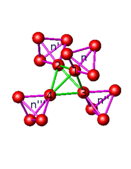
Figure 1: (Colour online) The face centred cubic (fcc) unit cell of Tb₂Ti₂O₇, showing only the Tb³⁺ ions and the exchange paths connecting them. There are two orientations of tetrahedra, which we call $A$ (green) and $B$ (pink). The lines connecting the ions (the edges of the tetrahedra) are the exchange paths. The labels on the ions (1-4) and the $A$ tetrahedra ($n$, $n^{\prime}$, $n^{\prime\prime}$, $n^{\prime\prime\prime\prime}$) illustrate how each ion on a $B$ tetrahedron also belongs to an $A$ tetrahedron.

The operator $H^{B}$ can also be expressed as a sum over A tetrahedra. Consider a particular B tetrahedron. Each of its four spins are located on the vertices of different A tetrahedra. If the spin on site #1 is on the $n$-th A tetrahedron, the spin on site #2 is on the $n^{\prime}$-th A tetrahedron, where $n^{\prime}\equiv n-(1/2,1/2,0)$, the spin on site #3 is on $n^{\prime\prime}\equiv n-(1/2,0,1/2)$, and the spin on site #4 is on $n^{\prime\prime\prime}\equiv n-(0,1/2,1/2)$, as shown in Fig. 1. Then

$$H^{B}=\sum_{n}H^{B}_{n}=\sum_{n}{\cal J}_{1}X_{1n}^{B}+{\cal J}_{2}X_{2n}^{B}+{\cal J}_{3}X_{3n}^{B}+{\cal J}_{4}X_{4n}^{B}$$ (18)

where, for example,

$$X_{1n}^{B} = -\frac{1}{3}(J_{n1z}J_{n^{\prime}2z}+J_{n1z}J_{n^{\prime\prime}3z}+J_{n1z}J_{n^{\prime\prime\prime}4z}$$ (19)

$$+ J_{n^{\prime}2z}J_{n^{\prime\prime}3z}+J_{n^{\prime}2z}J_{n^{\prime\prime\prime}4z}+J_{n^{\prime\prime}3z}J_{n^{\prime\prime\prime}4z}).$$

The exchange Hamilton for Tb₂Ti₂O₇, $H^{\rm Tb}_{\rm ex}$ (13), can be split into A and B parts in a similar way,

$$H_{\rm ex}^{\rm Tb}=H^{\rm A,Tb}+H^{\rm B,Tb}.$$ (20)

III.2 The spin-1/2 independent tetrahedra model

First we consider a simple model involving the exchange paths on a single tetrahedron (the $n$th A tetrahedron),

$$H^{A}_{n}={\cal J}_{1}X_{1n}^{A}+{\cal J}_{2}X_{2n}^{A}+{\cal J}_{3}X_{3n}^{A}+{\cal J}_{4}X_{4n}^{A}.$$ (21)

This can be represented as a $16\times 16$ matrix, which can be block diagonalised using the kets described in Appendix B. Exact eigenfunctions can easily be found.

The solutions to $H^{A}$ (15) are the direct product (over tetrahedra) of the single tetrahedron solutions of $H^{A}_{n}$ (21), which is why it is called the “independent tetrahedra model”. Because it is exactly solvable, $H^{A}$ is often used to model experiments instead of the full Hamiltonian $H_{\rm ex}$ (8).molavian2007 ; dalmas2012 ; curnoe2013 $H^{A}$ is a model that omits half of the exchange paths in $H_{\rm ex}$, which suggests that the exchange constants of $H^{A}$ are approximately twice as large as those of $H_{\rm ex}$.dalmas2012 We also note that $H^{A}$ has a lower symmetry than $H_{\rm ex}$: instead of the full space group $Fd\bar{3}m$, it is $F\bar{4}3m$, with point group $T_{d}$ instead of $O_{h}$.curnoe2008

III.3 The exchange interaction for Tb₂Ti₂O₇

III.3.1 The exchange interaction for non-Kramers spins restricted to the CEF ground state

When non-Kramers spins are restricted to the CEF ground state, the exchange interaction is greatly simplified because the matrix elements for $J_{\pm}$ vanish within this restriction. Then the eigenvectors are the classical states $|\pm\pm\pm\pm\pm\pm\ldots\rangle$. The ground state is either the doubly degenerate all-in-all-out state (${\cal I}_{1}>0$) or a highly degenerate spin ice state (${\cal I}_{1}<0$). This model maps to a spin-1/2 model with ${\cal J}_{1}=4{\cal I}_{1}j_{1}^{2}$ and ${\cal J}_{2,3,4}=0$. This model describes the spin ice material Ho₂Ti₂O₇, but it is insufficient for Tb₂Ti₂O₇, for which higher CEF levels must be included.

III.3.2 The exchange interaction for non-Kramers spins restricted to the CEF ground state and first excited state

Perturbation theory is used to determine the mixing of the first excited CEF level to the CEF ground state manifold. The unperturbed Hamiltonian is $H_{\rm{CEF}}$ (1) restricted to the CEF ground and first excited states, while the exchange interaction $H^{\rm Tb}_{\rm ex}$ (13) is the perturbation.

Second order perturbation theory yields an effective exchange Hamiltonian restricted to the CEF ground state:messiah

$$H^{\rm Tb}_{\rm eff}=PH^{\rm Tb}_{\rm ex}P+PH^{\rm Tb}_{\rm ex}\frac{Q}{a}H^{\rm Tb}_{\rm ex}P$$ (22)

where $P$ is the projector to the CEF ground state and $Q$ is the projector that is supplementary to $P$ i.e. it projects states that have one or more spins in the CEF first excited state. The denominator $a$ is the energy difference between the ground and excited states. $P$ is the direct product of projectors $P_{n}$ which operate on single tetrahedra. $Q$ can also be expressed in terms of single tetrahedron operators: on the $n$th tetrahedron, one, two, three or four spins can be excited, corresponding to the projections $Q_{n,{\rm one}}$, $Q_{n,{\rm two}}$ etc. However, for second order perturbation theory, we need only consider contributions to $Q$ where one or two spins are excited because $H^{\rm Tb}_{\rm ex}$ is bilinear in the spin operators and can only excite up to two spins at a time via the operators $J_{\pm}$ and $J_{z}$. Therefore,

$$\frac{Q}{a}=\sum_{n}\frac{Q_{n,{\rm one}}}{-\Delta}+\sum_{n}\frac{Q_{n,{\rm two}}}{-2\Delta}+\sum_{n,m<n}\frac{Q_{n,{\rm one}}Q_{m,{\rm one}}}{-2\Delta}$$ (23)

where the first term has one spin excited on one tetrahedron, the second term has two spins excited on one tetrahedron and the third term has two spins excited on two different tetrahedra. The operators $Q_{n,{\rm one}}$ and $Q_{n,{\rm two}}$ can be further expanded as

$$Q_{n,{\rm one}} = Q_{n1}P_{n2}P_{n3}P_{n4}+P_{n1}Q_{n2}P_{n3}P_{n4}+$$ (24)

$$P_{n1}P_{n2}Q_{n3}P_{n4}+P_{n1}P_{n2}P_{n3}Q_{n4}$$

$$Q_{n,{\rm two}} = Q_{n1}Q_{n2}P_{n3}P_{n4}+Q_{n1}P_{n2}Q_{n3}P_{n4}+$$ (25)

$$Q_{n1}P_{n2}P_{n3}Q_{n4}+P_{n1}Q_{n2}Q_{n3}P_{n4}+$$

$$P_{n1}Q_{n2}P_{n3}Q_{n4}+P_{n1}P_{n2}Q_{n3}Q_{n4}.$$

In Section IV, we show that $H^{\rm Tb}_{\rm eff}$ (22) has the same matrix representation as $H_{\rm ex}$ (8). However, before considering the full lattice exchange $H_{\rm eff}^{\rm Tb}$, we will study the simpler independent tetrahedra model.

III.3.3 The exchange interaction for non-Kramers spins in the independent tetrahedra model

In the independent tetrahedra model, the Hamiltonian for Tb³⁺ spins is $H^{A,{\rm Tb}}$. Perturbation theory yields

$$H^{A,{\rm Tb}}_{\rm eff} = PH^{A,{\rm Tb}}P+PH^{A,{\rm Tb}}\frac{Q}{a}H^{A,{\rm Tb}}P$$ (26)

$$= \sum_{n}PH^{A,{\rm Tb}}_{n}P+\sum_{n,m}PH^{A,{\rm Tb}}_{n}\frac{Q}{a}H^{A,{\rm Tb}}_{m}P$$

$$= \sum_{n}\left[PH^{A,{\rm Tb}}_{n}P\right.$$

$$\left.+PH^{A,{\rm Tb}}_{n}\left(\frac{Q_{n,{\rm one}}}{-\Delta}+\frac{Q_{n,{\rm two}}}{-2\Delta}\right)H^{A,{\rm Tb}}_{n}P\right]$$

$$\equiv \sum_{n}H_{n,{\rm eff}}^{A,{\rm Tb}}$$ (28)

In the second last line we make use of the fact that $H^{A,{\rm Tb}}_{n}$ acts only within the $n$th tetrahedron, so the only non-zero contribution in the sum over $n$ and $m$ is when $m=n$. Therefore this calculation reduces to a single tetrahedron Hamiltonian $H^{A,{\rm Tb}}_{n,{\rm eff}}$.

IV Map between spin-1/2 and Tb³⁺ exchange models

The results of the single tetrahedron calculation were found previously.curnoe2013 By comparing a matrix representation of $H^{A,{\rm Tb}}_{n,{\rm eff}}$ to a matrix representation of the spin-1/2 single tetrahedron $H^{A}_{n}$, a map between the Tb³⁺ exchange constants and the spin-1/2 exchange constants was found. The basis functions that were used to find the matrix representations are given in Appendix B (82 - 99). Here we follow a slightly different approach to the same result: instead of representing $H^{{\rm Tb}}_{\rm eff}$ (22) and $H_{\rm{ex}}$ (8) in the basis given by (82 - 99), we use the basis $\left|\pm\pm\pm\pm\right\rangle_{\frac{1}{2}}$ for the spin-1/2 states and the corresponding Tb³⁺ tetrahedron states determined by (7). The two approaches differ in the following way. When the basis (82 - 99) is used, matrix elements of the Hamiltonian are real, while (two of) the basis functions are complex. When the $|\pm\pm\pm\pm\rangle$ basis is used, the basis functions are real but the matrix elements of the Hamiltonian are complex. When the map (7) is applied, the Hamiltonian matrix must be complex-conjugated.

IV.1 Matrix representation of the spin-1/2 exchange Hamiltonian $H_{\rm ex}$

In the spin-1/2 case the following operators are replaced by the matrices:

$$J_{z} \rightarrow \frac{1}{2}\left(\begin{array}[]{cc}1&0\\ 0&-1\end{array}\right)\equiv\frac{1}{2}\sigma_{z}$$ (31)

$$J_{+} \rightarrow \left(\begin{array}[]{cc}0&1\\ 0&0\end{array}\right)\equiv S_{+}$$ (34)

$$J_{-} \rightarrow \left(\begin{array}[]{cc}0&0\\ 1&0\end{array}\right)\equiv S_{-}.$$ (37)

The product of operators associated with different sites is replaced by the Kronecker product of matrices. In this way, both the full spin-1/2 exchange Hamiltonian $H_{\rm ex}$ (8) and the spin-1/2 independent tetrahedra Hamiltonian $H^{A}$ (15) can be expressed as matrices by simply using the replacements (31-37).

IV.2 Matrix representation of the Tb³⁺ exchange Hamiltonian $H_{\rm eff}^{\rm Tb}$

In order to compare the matrix representation of the Tb³⁺ exchange Hamiltonian to the matrix representation of the spin-1/2 exchange Hamiltonian, the basis states $|\pm\pm\pm\pm\rangle_{\rm Tb}$ that are used to generate the Tb³⁺ matrix must match the order and relative phase of the basis states $|\pm\pm\pm\pm\rangle_{\frac{1}{2}}$ used to generate the spin-1/2 matrix, i.e., they must be ordered and signed according to (7) and the resulting matrices must be complex-conjugated. The results are then expressed in terms of the spin-1/2 matrices $\sigma_{z}$ and $S_{\pm}$. After following this procedure, we find that the various Tb³⁺ operators which appear in H${}_{\rm eff}^{\rm Tb}$ (22) are represented by the following spin-1/2 matrices:

$$PJ_{z}P \rightarrow -j_{1}\sigma_{z}$$ (38)

$$PJ_{\pm}P \rightarrow 0$$ (39)

$$PJ_{z}\frac{Q}{a}J_{z}P \rightarrow -\frac{j_{3}^{2}}{\Delta}$$ (40)

$$PJ_{+}\frac{Q}{a}J_{+}P \rightarrow 0$$ (41)

$$PJ_{+}\frac{Q}{a}J_{-}P \rightarrow -\frac{t^{2}}{2\Delta}(1+\sigma_{z})$$ (42)

$$PJ_{-}\frac{Q}{a}J_{+}P \rightarrow -\frac{t^{2}}{2\Delta}(1-\sigma_{z})$$ (43)

$$PJ_{1z}\frac{Q}{a}J_{1+}P \rightarrow -\frac{j_{3}t}{\Delta}S_{1-}\sigma_{2z}\sigma_{3z}\sigma_{4z}$$ (44)

$$= PJ_{1+}\frac{Q}{a}J_{1z}P$$ (45)

$$PJ_{1z}\frac{Q}{a}J_{1-}P \rightarrow -\frac{j_{3}t}{\Delta}S_{1+}\sigma_{2z}\sigma_{3z}\sigma_{4z}$$ (46)

$$= PJ_{1-}\frac{Q}{a}J_{1z}P.$$ (47)

The $2\times 2$ identity matrix is assumed when no matrix is given.

IV.2.1 Exchange interaction for Tb³⁺ spins in the independent tetrahedra model

Using the substitutions (38-47), the independent tetrahedra exchange Hamiltonian for Tb³⁺ spins $H^{A,{\rm Tb}}_{\rm eff}$ (28) can be expressed as a matrix. By direct comparison to the matrix representation of the spin-1/2 independent tetrahedra Hamitonian $H^{A}$, the following map between the exchange constants of spin-1/2 and the Tb³⁺ independent tetrahedra models can be inferred and previous resultscurnoe2013 are reproduced:

$${\cal J}_{1} = 4{\cal I}_{1}j_{1}^{2}+\frac{(4{\cal I}_{1}j_{1}j_{3})^{2}}{3\Delta}-\frac{(4{\cal I}_{2}j_{1}t)^{2}}{3\Delta}+\frac{({\cal I}_{3}t^{2})^{2}}{3\Delta}$$ (48)

$$-\frac{({\cal I}_{4}t^{2})^{2}}{12\Delta}$$

$${\cal J}_{2} = -\frac{4{\cal I}_{1}{\cal I}_{2}j_{1}^{2}j_{3}t}{3\Delta}$$ (49)

$${\cal J}_{3} = \frac{2({\cal I}_{2}j_{3}t)^{2}}{3\Delta}-\frac{{\cal I}_{1}{\cal I}_{3}j_{3}^{2}t^{2}}{3\Delta}$$ (50)

$${\cal J}_{4} = \frac{(2{\cal I}_{2}j_{3}t)^{2}}{3\Delta}+\frac{{\cal I}_{1}{\cal I}_{4}j_{3}^{2}t^{2}}{3\Delta}.$$ (51)

A constant offset was also found:

$${\cal C} = -\frac{(2{\cal I}_{1}j_{1}j_{3})^{2}}{3\Delta}-\frac{({\cal I}_{1}j_{3}^{2})^{2}}{3\Delta}-\frac{2(2{\cal I}_{2}j_{1}t)^{2}}{3\Delta}$$ (52)

$$-\frac{(2{\cal I}_{2}j_{3}t)^{2}}{3\Delta}-\frac{({\cal I}_{3}t^{2})^{2}}{6\Delta}-\frac{({\cal I}_{4}t^{2})^{2}}{24\Delta}.$$

IV.2.2 The full lattice exchange interaction for Tb³⁺ spins

We now consider the full exchange model $H^{\rm Tb}_{\rm eff}$ (22) for Tb³⁺ spins. We shall show that $H^{\rm Tb}_{\rm eff}$ is equivalent to the spin-1/2 exchange Hamiltonian $H_{\rm ex}$ (8) plus additional next-nearest-neighbour and fourth order in ${\vec{J}}$ interactions.

Both of the operators $H^{A,{\rm Tb}}$ and $H^{B,{\rm Tb}}$ appear in the expression for $H^{\rm Tb}_{\rm eff}$, which is expanded as:

$$H_{\rm eff}^{\rm Tb} = PH^{A,{\rm Tb}}P+PH^{A,{\rm Tb}}\frac{Q}{a}H^{A,{\rm Tb}}P+$$

$$PH^{B,{\rm Tb}}P+PH^{B,{\rm Tb}}\frac{Q}{a}H^{B,{\rm Tb}}P+$$

$$PH^{A,{\rm Tb}}\frac{Q}{a}H^{B,{\rm Tb}}P+PH^{B,{\rm Tb}}\frac{Q}{a}H^{A,{\rm Tb}}P.$$

The first two terms were already considered in the discussion of independent tetrahedra model $H^{A,{\rm Tb}}_{\rm eff}$ (28), and they correspond to the term $H^{A}$ in $H_{\rm ex}$ (14). The third and fourth terms correspond to $H^{B}$ in $H_{\rm ex}$. It is obvious from symmetry considerations that the constants of the effective spin-1/2 model for $H^{B}$ (18) should be the same as those found for $H^{A}$ (15). The sum of the first four terms therefore corresponds to $H_{\rm ex}$ (8,14), with effective coupling constants as given by (48-52).

The last two terms of (LABEL:HTbeff2) yield additional next-nearest-neighbour (n.n.n.) interactions, and some unusual fourth order (in $\vec{J}$) interactions. Symmetry considerations determine the most general form of these interactions. When the two interacting spins are at different site numbers then the interaction takes the same general form as $H_{\rm ex}$ (8,9-12), except that the sum is over pairs of next-nearest neighbours with different site numbers, $s_{i}\neq s_{j}$. These four contributions will be denoted $X_{i}^{\prime}$, $i=1,2,3,4$. In addition, there are two interaction terms between spins that are next-nearest-neighbours with the same site number ($s_{i}=s_{i^{\prime}}$), for a total of 6 n.n.n. exchange coupling constants:

$$H_{\rm ex,n.n.n.} = {\cal J}_{1}^{\prime}X_{1}^{\prime}+{\cal J}^{\prime}_{2}X_{2}^{\prime}+{\cal J}_{3}^{\prime}X_{3}^{\prime}+{\cal J}_{4}^{\prime}X_{4}^{\prime}+$$ (54)

$${\cal J}^{\prime}_{5}X_{5}^{\prime}+{\cal J}_{6}^{\prime}X_{6}^{\prime}$$

where

$$X_{5}^{\prime} = \sum_{\langle\langle i,i^{\prime}\rangle\rangle}J_{iz}J_{i^{\prime}z}\;\;\mbox{($s_{i}=s_{i^{\prime}}$)}$$ (55)

$$X_{6}^{\prime} = \frac{1}{2}\sum_{\langle\langle i,i^{\prime}\rangle\rangle}J_{i+}J_{i^{\prime}-}+J_{i-}J_{i^{\prime}+}\;\;\mbox{($s_{i}=s_{i^{\prime}}$)}.$$ (56)

Among the many different fourth order in $\vec{J}$ terms which may appear in $H_{\rm eff}^{\rm Tb}$, the ones that are produced by the last two terms of (LABEL:HTbeff2) are

$$H_{\rm ex,4-order}={\cal J}^{\prime}_{7}X_{7}^{\prime}+{\cal J}^{\prime}_{8}X^{\prime}_{8}$$ (57)

where

$$X_{7}^{\prime} = \sum_{\langle i,j,k,l\rangle}\Lambda_{ijkl}J_{i+}J_{jz}J_{kz}J_{lz}+J_{i-}J_{jz}J_{kz}J_{lz}$$ (58)

$$X_{8}^{\prime} = \sum_{\langle i,j,l,i^{\prime}\rangle}\Lambda_{ijki}J_{i+}J_{jz}J_{kz}J_{i^{\prime}z}.$$ (59)

In $X_{7}^{\prime}$, the sites $i,j,k,l$ have different site numbers. Three of the sites ($i$, $j$, $k$) form a triangle, and the fourth site $l$ is connected to the triangle by a nearest neighbour bond (but it does not complete a tetrahedron). In $X_{8}^{\prime}$, the sites $i,j,k$ have different site numbers. They are arranged in a triangle, while the fourth site $i^{\prime}$ has the same site number as the site $i$ and is connected to the triangle by a nearest neighbour bond. Examples of arrangements of ions involved in these interactions are shown in Fig. 2. Similar to the expressions for $X_{2}$ and $X_{3}$, the phases $\Lambda_{ijkl}$ are fixed by symmetry considerations with values of either 1, $\varepsilon$ or $\varepsilon^{2}$.

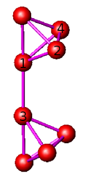
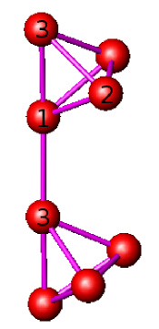
Figure 2: (Colour online) Examples of arrangements of ions involved in fourth order exchange terms. The left diagram corresponds to $X^{\prime}_{7}$ and the right to $X^{\prime}_{8}$.

Matrix representations for $H_{\rm ex,n.n.n.}$ (54) and $H_{\rm ex,4-order}$ (57) can be written using the substitutions (31-37). By comparing these with the matrix representation of $H_{\rm eff}^{\rm Tb}$, the constants ${\cal J}_{i}^{\prime}$ can be inferred:

$${\cal J}_{2,3,4,6}^{\prime} = 0$$ (60)

$${\cal J}_{1}^{\prime} = \frac{2(2{\cal I}_{1}j_{1}j_{3})^{2}}{3\Delta}-\frac{2(2{\cal I}_{2}j_{1}t)^{2}}{3\Delta}$$ (61)

$${\cal J}_{5}^{\prime} = -\frac{2(2{\cal I}_{1}j_{1}j_{3})^{2}}{9\Delta}-\frac{(4{\cal I}_{2}j_{1}t)^{2}}{9\Delta}$$ (62)

$${\cal J}_{7}^{\prime} = \frac{32\sqrt{2}{\cal I}_{1}{\cal I}_{2}j_{1}^{2}j_{3}t}{9\Delta}$$ (63)

$${\cal J}_{8}^{\prime} = -\frac{16\sqrt{2}{\cal I}_{1}{\cal I}_{2}j_{1}^{2}j_{3}t}{9\Delta}.$$ (64)

In summary, we have considered two different exchange models for Tb³⁺ spins in Tb₂Ti₂O₇, the independent tetrahedra model and the full lattice model. The maps for these models onto spin-1/2 exchange models can be illustrated schematically as

Tb₂Ti₂O₇ spin-1/2 independent tetrahedron $\rightarrow$ independent tetrahedron anisotropic exchange anisotropic exchange spin-1/2 Tb₂Ti₂O₇ full lattice full lattice $\rightarrow$ anisotropic exchange anisotropic exchange plus next-nearest neighbour and four-body interactions.

The relation between the anisotropic nearest-neighbour exchange constants, given by (48-51), is the same for both models.

V Discussion

Recent magnetisation measurements on Tb₂Ti₂O₇ have been performed by a few groups [legl2012, ; lhotel2012, ; sazonov2013, ]. In the presence of a magnetic field, the Hamiltonian for Tb₂Ti₂O₇ is

$$H({\vec{B}})=H_{\rm CEF}+H_{\rm ex}^{\rm Tb}+\sum_{i}\mu_{B}g_{J}\vec{J}_{i}\cdot\vec{B}$$ (65)

where $g_{J}=\frac{3}{2}$ is the Landé $g$-factor for Tb³⁺ and $\mu_{B}$ is the Bohr magneton. Being unsolvable, $H({\vec{B}})$ is normally handled using either a self-consistent mean field approximation or by using the independent tetrahedron model. Both of these methods involve considerable simplifications of $H(\vec{B})$. In the former, nearest neighbour exchange interactions are replaced by an effective mean field, and the problem is reduced to the solution of a single ion Hamiltonian. In the latter, a single tetrahedron is solved but correlations between tetrahedra are omitted.

Using the mean field approach, approximate values for the exchange constants for Tb₂Ti₂O₇ were obtained.sazonov2013 The relation between the exchange constants used in Ref. sazonov2013, and those defined by (8,9-12) is given in Appendix C. Using our definitions, the constants are (in kelvin)

$${\cal I}_{1} = -.128$$ (66)

$${\cal I}_{2} = -.083$$ (67)

$${\cal I}_{3} = -.1595$$ (68)

$${\cal I}_{4} = -.281$$ (69)

It should be noted that in Ref. sazonov2013, a constraint was applied in determining these numbers (it was assumed that the anti-symmetric exchange term was absent), such that in effect only three parameters within the four parameter space were explored. Nevertheless, these numbers can provide estimates of the exchange constants for the effective spin-1/2 model. Ref. sazonov2013, uses CEF states derived from the CEF Hamiltonian in Ref. mirebeau2007, , with matrix elements $j_{1}=-3.4$, $j_{2}=4.3$, $j_{3}=-2.0$, $t=4.65$ (defined by Eqs. (3-6)) and $\Delta=18.24$ K. Among all the exchange constants for the spin-1/2 model, only ${\cal J}_{1}$ has a first order in perturbation theory correction; the rest are non-zero only in second order. Using Eq. 48, and the numbers given above, we calculate ${\cal J}_{1}\approx-6.1$. The other constants are calculated using (49-51), which yields ${\cal J}_{2}\approx.085$, ${\cal J}_{3}\approx-0.011$ and ${\cal J}_{4}\approx 0.10$; however, without more accurate knowledge of the Tb₂Ti₂O₇ exchange constants, these values are likely not very meaningful. The values obtained in Ref. curnoe2013, , also highly approximate, are in rough agreement, ${\cal J}_{1}\approx-5.1$, ${\cal J}_{2}\approx 0.2$, ${\cal J}_{3}\approx 0.1$ and ${\cal J}_{4}\approx 0.3$.

The negative sign of ${\cal J}_{1}$ indicates that Tb₂Ti₂O₇ is a spin-1/2 spin ice, with quantum fluctuations arising from the other terms in $H_{\rm ex}$, in agreement with recent observations of spin ice-like correlations in Tb₂Ti₂O₇.fennell2012 ; fritsch2013 It will be interesting to see how magnetic monopoles, which are postulated to exist as excitations in spin ices,castelnovo2008 may be manifested in Tb₂Ti₂O₇.

Using either set of estimates for the exchange constants given above to locate the position of Tb₂Ti₂O₇ in the phase diagrams presented in Refs. savary2012a, and lee2012, , the ground state of Tb₂Ti₂O₇ is predicted to be a “quantum spin liquid” (QSL), or possibly a “Coulomb ferromagnet” (CFM) close to the QSL boundary. Both of these are highly entangled quantum mechanical states, with the CFM state distinguishable from the QSL state by a non-zero magnetisation. However, a complete description of Tb₂Ti₂O₇ is almost certainly more complicated due to interactions with lattice structuremaczka2008 ; bonville2014 or elastic strain.aleksandrov1981 ; aleksandrov1985 ; mamsurova1986 ; ruff2007 ; ruff2010 ; luan2011 ; nakanishi2011 ; fennell2014

VI Summary

Symmetry-based analysis (group theory) is a powerful means of reducing the complexity of highly symmetric crystals with limited degrees of freedom. The observation that non-Kramers doublets and a spin-1/2 spinors possess the same symmetry when considered in groups of four (the four vertices of a tetrahedron in the pyrochlore lattice) is unexpected, non-trivial, and very useful. It defines a map between non-Kramers Tb³⁺ and spin-1/2 basis states, which in turn provides the basis for a map between the exchange interaction specific to Tb₂Ti₂O₇ and a generic spin-1/2 model. Furthermore, the map easily incorporates (via perturbation theory) the effects of a low-lying crystal electric field excited state. However, in order to calculate the spin-1/2 anisotropic exchange constants with quantitative accuracy, precise determinations of the anisotropic exchange constants and the CEF Hamiltonian for Tb₂Ti₂O₇ are essential.

Appendix A Local axes for rare earth ions in pyrochlore crystals

For site #1, the local $z$-axis is parallel to the $[111]$ direction and the local $x$- and $y$-axes are chosen to be perpendicular to $z$ and to obey the right hand rule. These local axes define a set of magnetic operators

$$J_{1x} = (J_{1}^{x}+J_{1}^{y}-2J_{1}^{z})/\sqrt{6}$$ (70)

$$J_{1y} = (-J_{1}^{x}+J_{1}^{y})/\sqrt{2}$$ (71)

$$J_{1z} = (J_{1}^{x}+J_{1}^{y}+J_{1}^{z})/\sqrt{3}$$ (72)

where subscripts are used for operators using local axes and superscripts for global axes.

Local axes for site #2 are defined by rotating the #1 axes by $C_{2z}$ (this operation also exchanges sites #1 and #2):

$$J_{2x} = (-J_{2}^{x}-J_{2}^{y}-2J_{2}^{z})/\sqrt{6}$$ (73)

$$J_{2y} = (J_{2}^{x}-J_{2}^{y})/\sqrt{2}$$ (74)

$$J_{2z} = (-J_{2}^{x}-J_{2}^{y}+J_{2}^{z})/\sqrt{3}.$$ (75)

Similarly, local axes for site #3 are defined by rotating the #1 axes by $C_{2y}$:

$$J_{3x} = (-J_{3}^{x}+J_{3}^{y}+2J_{3}^{z})/\sqrt{6}$$ (76)

$$J_{3y} = (J_{3}^{x}+J_{3}^{y})/\sqrt{2}$$ (77)

$$J_{3z} = (-J_{3}^{x}+J_{3}^{y}-J_{3}^{z})/\sqrt{3}.$$ (78)

Finally, local axes for site #4 are defined by rotating #1 axes by $C_{2x}$:

$$J_{4x} = (J_{4}^{x}-J_{4}^{y}+2J_{4}^{z})/\sqrt{6}$$ (79)

$$J_{4y} = (-J_{4}^{x}-J_{4}^{y})/\sqrt{2}$$ (80)

$$J_{4z} = (J_{4}^{x}-J_{4}^{y}-J_{4}^{z})/\sqrt{3}.$$ (81)

Appendix B Tetrahedron basis functions

A suitable set of basis functions for the non-Kramers doublet that transform according to the irreducible representations $A_{1}\oplus 3E\oplus 2T_{1}\oplus T_{2}$ iscurnoe2007 ; curnoe2013

$$(|A_{1}\rangle = (|++--\rangle+|+-+-\rangle+|+--+\rangle+|--++\rangle+|-+-+\rangle+|-++-\rangle)/\sqrt{6}$$ (82)

$$|E_{+}^{(1)}\rangle = -|----\rangle,\;\;\;|E_{-}^{(1)}\rangle=-|++++\rangle$$ (83)

$$|E_{+}^{(2)}\rangle = (|-+++\rangle+|+-++\rangle+|++-+\rangle+|+++-\rangle)/2$$ (84)

$$|E_{-}^{(2)}\rangle = (|+---\rangle+|-+--\rangle+|--+-\rangle+|---+\rangle)/2$$ (85)

$$|E_{+}^{(3)})\rangle = (|++--\rangle+\varepsilon^{2}|+-+-\rangle+\varepsilon|+--+\rangle+|--++\rangle+\varepsilon^{2}|-+-+\rangle+\varepsilon|-++-\rangle)/\sqrt{6}$$ (86)

$$|E_{-}^{(3)}\rangle = (|++--\rangle+\varepsilon|+-+-\rangle+\varepsilon^{2}|+--+\rangle+|--++\rangle+\varepsilon|-+-+\rangle+\varepsilon^{2}|-++-\rangle)/\sqrt{6}$$ (87)

$$|T_{1z}^{(1)}\rangle = (|+++-\rangle+|++-+\rangle-|+-++\rangle-|-+++\rangle+|+---\rangle+|-+--\rangle-|--+-\rangle$$ (88)

$$-|---+\rangle)/2\sqrt{2}$$

$$|T_{1z}^{(2)}\rangle = (|--++\rangle-|++--\rangle)/\sqrt{2}$$ (89)

$$|T_{2z}\rangle = -(|+++-\rangle+|++-+\rangle-|+-++\rangle-|-+++\rangle-|+---\rangle-|-+--\rangle+|--+-\rangle$$ (90)

$$+|---+\rangle)/2\sqrt{2}.$$

The states $|T_{1,2x}\rangle$ and $T_{1,2y}\rangle$ can be found by rotating $|T_{1,2z}\rangle$. The corresponding spin-1/2 tetrahedron states can be found using (7). They are

$$|A_{1}\rangle = (|++--\rangle+|+-+-\rangle+|+--+\rangle+|--++\rangle+|-+-+\rangle+|-++-\rangle)/\sqrt{6}$$ (91)

$$|E_{+}^{(1)}\rangle = |++++\rangle,\;\;\;|E_{-}^{(1)}\rangle=|----\rangle$$ (92)

$$|E_{+}^{(2)}\rangle = (|+---\rangle+|-+--\rangle+|--+-\rangle+|---+\rangle)/2$$ (93)

$$|E_{-}^{(2)}\rangle = -(|-+++\rangle+|+-++\rangle+|++-+\rangle+|+++-\rangle)/2$$ (94)

$$|E_{+}^{(3)}\rangle = (|++--\rangle+\varepsilon|+-+-\rangle+\varepsilon^{2}|+--+\rangle+|--++\rangle+\varepsilon|-+-+\rangle+\varepsilon^{2}|-++-\rangle)/\sqrt{6}$$ (95)

$$|E_{-}^{(3)}\rangle = (|++--\rangle+\varepsilon^{2}|+-+-\rangle+\varepsilon|+--+\rangle+|--++\rangle+\varepsilon^{2}|-+-+\rangle+\varepsilon|-++-\rangle)/\sqrt{6}$$ (96)

$$|T_{1z}^{(1)}\rangle = (|+++-\rangle+|++-+\rangle-|+-++\rangle-|-+++\rangle-|+---\rangle-|-+--\rangle+|--+-\rangle$$ (97)

$$+|---+\rangle)/2\sqrt{2}$$

$$|T_{1z}^{(2)}\rangle = (|++--\rangle-|--++\rangle)/\sqrt{2}$$ (98)

$$|T_{2z}\rangle = (|+++-\rangle+|++-+\rangle-|+-++\rangle-|-+++\rangle+|+---\rangle+|-+--\rangle-|--+-\rangle$$ (99)

$$-|---+\rangle)/2\sqrt{2}.$$

As described elsewhere,curnoe2013 using the spin-1/2 single tetrahedron states, $H^{A}_{n}$ can be represented as a block matrix, with the eigenvalues ${\cal J}_{1}/6-2{\cal J}_{4}/3$ and $-2{\cal J}_{3}/3+{\cal J}_{4}/6$ in the $A_{1}$ and $T_{2}$ sectors, and the matrices

$$\left(\begin{array}[]{ccc}-\frac{{\cal J}_{2}}{2}&0&\frac{\sqrt{2}{\cal J}_{3}}{\sqrt{3}}\\ 0&-\frac{{\cal J}_{4}}{2}&-\frac{2{\cal J}_{2}}{\sqrt{3}}\\ \frac{\sqrt{2}{\cal J}_{3}}{\sqrt{3}}&-\frac{2{\cal J}_{2}}{\sqrt{3}}&\frac{{\cal J}_{1}}{6}+\frac{{\cal J}_{4}}{3}\end{array}\right)\mbox{ and }\left(\begin{array}[]{cc}\frac{2{\cal J}_{3}}{3}+\frac{{\cal J}_{4}}{6}&\frac{2\sqrt{2}{\cal J}_{2}}{3}\\ \frac{2\sqrt{2}{\cal J}_{2}}{3}&\frac{{\cal J}_{1}}{6}\end{array}\right)$$

in the $E$ and $T_{1}$ sectors. The $E$ sector is doubly degenerate while the $T_{1}$ and $T_{2}$ sectors are triply degenerate.

Appendix C Alternate definitions of the exchange constants

Several different choices of definitions of the four anisotropic nearest neighbour exchange constants have appeared in the literature. This article uses the same definitions as in [curnoe2008, ; mcclarty2009, ; dalmas2012, ] with exchange constants denoted as ${\cal J}_{1}$, ${\cal J}_{2}$, ${\cal J}_{3}$ and ${\cal J}_{4}$.

The constants used in [ross2011, ; savary2012a, ; savary2012b, ; lee2012, ], denoted $J_{zz}$, $J_{z\pm}$, $J_{\pm\pm}$ and $J_{\pm}$, are proportional to the constants used in this work:

$${\cal J}_{1} = -3J_{zz}$$ (100)

$${\cal J}_{2} = 3J_{z\pm}/\sqrt{2}$$ (101)

$${\cal J}_{3} = 3J_{\pm\pm}$$ (102)

$${\cal J}_{4} = 6J_{\pm}.$$ (103)

The constants used in the magnetisation study by Sazonov et al. (Ref. sazonov2013, ), denoted ${\cal J}^{u}$, ${\cal J}^{v}$, ${\cal J}^{w}$ and ${\cal D}$, are defined in Ref. petit2012, . The relation between them and the constants used in this work is

$${\cal J}_{1} = -{\cal J}^{u}+2{\cal J}^{w}-2\sqrt{2}{\cal D}$$ (104)

$${\cal J}_{2} = {\cal J}^{u}/2+{\cal J}^{w}/2+{\cal D}/(2\sqrt{2})$$ (105)

$${\cal J}_{3} = {\cal J}^{u}/2+3{\cal J}^{v}/4-{\cal J}^{w}/4-{\cal D}/\sqrt{2}$$ (106)

$${\cal J}_{4} = -{\cal J}^{u}+3{\cal J}^{v}/2+{\cal J}^{w}/2+\sqrt{2}{\cal D}.$$ (107)

Since ${\cal J}_{i}$ are reserved for spin-1/2 models, the constants ${\cal I}_{1}$, ${\cal I}_{2}$, ${\cal I}_{3}$ and ${\cal I}_{4}$ are used instead for Tb₂Ti₂O₇. Using the results obtained in [petit2012, ; sazonov2013, ], $({\cal J}^{u},{\cal J}^{v},{\cal J}^{w},{\cal D})=(-.068,-.2,-.098,0)$ K, we calculate the results given in (66)-(69).

For completeness, we also include the constants used in [zhitomirsky2012, ; zhitomirsky2014, ], denoted $J_{zz}$, $J_{z\perp}$, $J_{\perp}$ and $J_{\perp}^{a}$:

$${\cal J}_{1} = -3J_{zz}$$ (108)

$${\cal J}_{2} = -\sqrt{3}J_{z\perp}/(2\sqrt{2})$$ (109)

$${\cal J}_{3} = J_{\perp}-J_{\perp}^{a}/4$$ (110)

$${\cal J}_{4} = J_{\perp}+J_{\perp}^{a}/2.$$ (111)

References

• (1) J. D. M. Champion, M. J. Harris, P. C. W. Holdsworth, A. S. Wills, G. Balakrishnan, S. T. Bramwell, E. Čižmár, T. Fennell, J. S. Gardner, J. Lago, D. F. McMorrow, M. Orendáč, A. Orendáčová, D. McK. Paul, R. I. Smith, M. T. F. Telling, and A. Wildes, Phys. Rev. B 68, 020401(R) (2003).
• (2) M. J. Harris, S. T. Bramwell, D. F. McMorrow, T. Zeiske and K. W. Godfrey, Phys. Rev. Lett. 79, 2554 (1997).
• (3) A. P. Ramirez, A. Hayashi, R. J. Cava, R. Siddharthan and B. S. Shastry, Nature 399, 333 (1999).
• (4) J. S. Gardner, B. D. Gaulin, A. J. Berlinsky, P. Waldron, S. R. Dunsiger, N. P. Raju and J. E. Greedan, Phys. Rev. B 64, 224416 (2001).
• (5) M. J. P. Gingras, B. C. den Hertog, M. Faucher, J. S. Gardner, S. R. Dunsiger, L. J. Chang, B. D. Gaulin, N. P. Raju and J. E. Greedan, Phys. Rev. B 62, 6496 (2000).
• (6) I. Mirebeau, P. Bonville and M. Hennion, Phys. Rev. B 76, 184436 (2007).
• (7) A. Bertin, Y. Chapuis, P. Dalmas de Réotier and A. Yaouanc, J. Phys.: Condens. Matter 24, 256003 (2012).
• (8) J. Zhang, K. Fritsch, Z. Hao, B. V. Bagheri, M. J. P. Gingras, G. E. Granroth, P. Jiramongkolchai, R. J. Cava, and B. D. Gaulin, Phys. Rev. B 89, 134410 (2014).
• (9) I. V. Aleksandrov, L. G. Mamsurova, K. K. Pukhov, N. G. Trusevich and L. G. Shcherbakova, JETP Lett. 34, 62 (1981).
• (10) I. V. Aleksandrov, B. V. Lidskii, L. G. Mamsurova, M. G. Neigauz, K. S. Pigal’skii, K. K. Pukhov, N. G. Trusevich and L. G. Shcherbakova, Sov. Phys. JETP 62, 1287 (1985).
• (11) S. H. Curnoe, Phys. Rev. B 78, 094418 (2008).
• (12) H. R. Molavian, M. J. P. Gingras and B. Canals, Phys. Rev. Lett. 98, 157204 (2007).
• (13) P. Dalmas de Réotier, A. Yaouanc, Y. Chapuis, S. H. Curnoe, B. Grenier, E. Ressouche, C. Marin, J. Lago, C. Baines and S. R. Giblin, Phys. Rev. B 86, 104424 (2012).
• (14) S. H. Curnoe, Phys. Rev. B 88, 014429 (2013).
• (15) A. Messiah, Quantum Mechanics, chap. XVI (Wiley, 1958).
• (16) S. Legl, C. Krey, S. R. Dunsiger, H. A. Dabkowska, J. A. Rodriguez, G. M. Luke and C. Pfleiderer, Phys. Rev. Lett. 109, 047201 (2012).
• (17) E. Lhotel, C. Paulson, P. Dalmas de Réotier, A. Yaouanc, C. Marin and S. Vanishri, Phys. Rev. B 86, 020410(R) (2012).
• (18) A. P. Sazonov, A. Gukasov, H. B. Cao, P. Bonville, E. Ressouche, C. Decorse and I. Mirebeau, Phys. Rev. B 88, 184428 (2013).
• (19) T. Fennell, M. Kenzelmann, B. Roessli, M. K. Haas and R. J. Cava, Phys. Rev. Lett. 109, 017201 (2012).
• (20) K. Fritsch, K. A. Ross, Y. Qiu, J. R. D. Copley, T. Guidi, R. I. Bewley, H. A. Dabkowska and B. D. Gaulin, Phys. Rev. B 87, 094410 (2013).
• (21) C. Castelnovo, R. Moessner and S. L. Sondhi, Nature 451, 42 (2008).
• (22) L. Savary and L. Balents, Phys. Rev. Lett. 108, 037202 (2012).
• (23) S. B. Lee, S. Onoda and L. Balents, Phys. Rev. B 86, 104412 (2012).
• (24) M. Ma̧czka, M. L. Sanjuán, A. F. Fuentes, K. Hermanowicz and J. Hanuza, Phys. Rev. B 78, 134420 (2008).
• (25) P. Bonville, A. Gukasov, I. Mirebeau and S. Petit, Phys. Rev. B 89, 085115 (2014).
• (26) L. G. Mamsurova, K. S. Pigal’skĩi and K. K. Pukhov, JETP Lett. 43, 755 (1986).
• (27) J. P. C. Ruff, B. D. Gaulin, J. P. Castellan, K. C. Rule, J. P. Clancy, J. Rodriguez and H. A. Dabkowska, Phys. Rev. Lett. 99, 237202 (2007).
• (28) J. P. C. Ruff, Z. Islam, J. P. Clancy, K. A. Ross, H. Nojiri, Y. H. Matsuda, H. A. Dabkowska, A. D. Dabkowski and B. D. Gaulin, Phys. Rev. Lett. 105, 077203 (2010).
• (29) Y. Luan, Elastic properties of complex transition metal oxides studied by Resonant Ultrasound Spectroscopy, Ph. D. thesis (University of Tennessee, 2011).
• (30) Y. Nakanishi, T. Kumagai, M. Yoshizawa, K. Matsuhira, S. Takagi and Z. Hiroi, Phys. Rev. B 83, 184434 (2011).
• (31) T. Fennell, M. Kenzelmann, B. Roessli, H. Mutka, J. Ollivier, M. Ruminy, U. Stuhr, O. Zaharko, L. Bovo, A. Cervellino, M. K. Haas and R. J. Cava, Phys. Rev. Lett. 112, 017203 (2014).
• (32) S. H. Curnoe, Phys. Rev. B 75, 212404 (2007).
• (33) P. A. McClarty, S. H. Curnoe and M. J. P. Gingras, J. Phys.: Conference Series 145, 012032 (2009).
• (34) K. A. Ross, L. Savary, B. D. Gaulin and L. Balents, Phys. Rev. X 1, 021002 (2011).
• (35) L. Savary, K. A. Ross, B. D. Gaulin, J. P. C. Ruff and L. Balents, Phys. Rev. Lett. 109, 167201 (2012).
• (36) S. Petit, P. Bonville, J. Robert, C. Decorse and I. Mirebeau, Phys. Rev. B 86, 174403 (2012).
• (37) M. E. Zhitomirsky, M. V. Gvozdikova, P. C. W. Holdsworth and R. Moessner, Phys. Rev. Lett. 109, 077204 (2012).
• (38) M. E. Zhitomirsky, P. C. W. Holdsworth and R. Moessner, Phys. Rev. B 89, 140403(R) (2014).