Magnetic energy dissipation and mean magnetic field generation in planar convection driven dynamos

Abstract

A numerical study of dynamos in rotating convecting plane layers is presented which focuses on magnetic energies and dissipation rates, and the generation of mean fields (where the mean is taken over horizontal planes). The scaling of the magnetic energy with the flux Rayleigh number is different from the scaling proposed in spherical shells, whereas the same dependence of the magnetic dissipation length on the magnetic Reynolds number is found for the two geometries. Dynamos both with and without mean field exist in rapidly rotating convecting plane layers.

It is generally assumed that celestial bodies without a fossil magnetic field left over form the birth of the object create their magnetic fields through the dynamo effect, and that in most bodies, convection is driving the motion of the fluid conductor whose kinetic energy is transformed into magnetic energy by the dynamo effect. Spherical shells and plane layers are two geometries in which convection driven dynamos are conveniently studied with numerical simulations. More attention has been paid to the spherical shell because of its greater geo- and astrophysical relevance and a larger data base exists for this geometry. A scaling for the magnetic field energy derived from these simulations Christensen and Aubert (2006) has matched observations well Christensen et al. (2009) and has even been invoked for mechanically driven dynamos Dwyer et al. (2011); Le Bars et al. (2011), which raises the question of how universal this scaling is. An obvious test is to compare convection dynamos in spherical shells with the most closely related standard problem, which is convection driven dynamos in plane layers. Rotating convection in spherical shells is inhomogeneous in the sense that the region inside the cylinder tangent to the inner core and coaxial with the rotation axis behaves differently from the equatorial region, and boundaries are curved. Convection in a plane layer with its rotation axis perpendicular to the plane of the layer may be viewed as a model for a small region surrounding the poles of a spherical shell. Are the physics in this region representative for the rest? This question is the motivation to look at the scaling of magnetic energy and energy dissipation in plane layer dynamos and to compare the results with data from simulations in spherical shells.

Field morphologies are more difficult to compare. Dynamos in spherical shells are frequently classified according to whether they produce a magnetic field dominated by its dipole component (in which case they are a candidate for a model of the geodynamo) or not. A similar distinction can be made among plane layer dynamos: They either produce a mean field, obtained by averaging over horizontal planes, or not. Even though this issue is not obviously analogous to the question of the dominating dipole field in the sphere, the end of this paper will be devoted to showing that a transition in plane layer dynamos separates dynamos generating mean fields from those who do not.

The model and the numerical method used here are the same as in ref. Tilgner, 2012 and are briefly reviewed here for completeness. The parameters of the numerical runs are the same, too, except for some additional simulations at larger aspect ratios. Consider a plane layer with boundaries perpendicular to the $z$ axis. Rotation $\Omega$ and gravitational acceleration $g$ are parallel and antiparallel to this axis, respectively. The fluid in the layer has density $\rho$, kinematic viscosity $\nu$, thermal diffusivity $\kappa$, thermal expansion coefficient $\alpha$, and magnetic diffusivity $\lambda$. The boundaries are located in the planes $z=0$ and $z=d$ and periodic boundary conditions are applied in the lateral directions imposing the periodicity lengths $l_{x}$ and $l_{y}$ along the $x$ and $y$ directions. In all simulations, $l_{x}=l_{y}$, and the aspect ratio $A$ is defined as $A=l_{x}/d$. Four additional control parameters govern magnetic rotating convection within the Boussinesq approximation, namely the Rayleigh number $\mathrm{Ra}$, the Ekman number $\mathrm{Ek}$, the Prandtl number $\mathrm{Pr}$, and the magnetic Prandtl number $\mathrm{Pm}$. They are defined by

$$\mathrm{Ra}=\frac{g\alpha\Delta Td^{3}}{\kappa\nu}~{}~{}~{},~{}~{}~{}\mathrm{Ek}=\frac{\nu}{\Omega d^{2}}~{}~{}~{},~{}~{}~{}\mathrm{Pr}=\frac{\nu}{\kappa}~{}~{}~{},~{}~{}~{}\mathrm{Pm}=\frac{\nu}{\lambda}$$ (1)

where $\Delta T$ is the temperature difference between bottom and top boundaries. With $d$, $d^{2}/\kappa$, $\kappa/d$, $\rho\kappa^{2}/d^{2}$, $\Delta T$ and $\sqrt{\mu_{0}\rho}\kappa/d$ as units of length, time, velocity, pressure, temperature difference from the temperature at $z=d$, and magnetic field, respectively, the nondimensional equations for the velocity field $\bm{v}(\bm{r},t)$ as a function of position $\bm{r}$ and time $t$, the magnetic field $\bm{B}(\bm{r},t)$ and the temperature field $T(\bm{r},t)$, are given by:

$$\partial_{t}\rho+\nabla\cdot\bm{v}=0$$ (2)

$$\begin{split}\partial_{t}\bm{v}+(\bm{v}\cdot\nabla)\bm{v}+2\frac{\mathrm{Pr}}{\mathrm{Ek}}\hat{\bm{z}}\times\bm{v}=\\ -c^{2}\nabla\rho+\mathrm{Pr}~{}\mathrm{Ra}~{}\theta\hat{\bm{z}}+\mathrm{Pr}\nabla^{2}\bm{v}+(\nabla\times\bm{B})\times\bm{B}\end{split}$$ (3)

$$\partial_{t}\theta+\bm{v}\cdot\nabla\theta-v_{z}=\nabla^{2}\theta$$ (4)

$$\partial_{t}\bm{B}+\nabla\times(\bm{B}\times\bm{v})=\frac{\mathrm{Pr}}{\mathrm{Pm}}\nabla^{2}\bm{B}$$ (5)

$$\nabla\cdot\bm{B}=0$$ (6)

where $\theta$ is the deviation from the conductive temperature profile. The numerical code implements an artificial compressibility method Chorin (1967) with the equation of state $p=c^{2}\rho$, with pressure $p$ and sound speed $c$. The standard Boussinesq equations, with eq. (2) replaced by $\nabla\cdot\bm{v}=0$ and with the term $-c^{2}\nabla\rho$ replaced by $\nabla p$ in eq. (3), are recovered in the limit of $c$ tending to infinity. In all simulations, $c$ was chosen large enough to approximate well the Boussinesq equations Tilgner (2012).

Eq. (2) is the full continuity equation linearized around a density equal to 1, $\rho$ being the density perturbation. Only $\nabla\rho$ enters the momentum equation so that we can set the unperturbed density to an arbitrary constant. The system with the linearized continuity equation reduces to the same Boussinesq limit for $c$ tending to infinity as the full system, it also satisfies conservation of mass, and it is computationally more efficient because it avoids round off errors in the term $1+\rho$ appearing in the full continuity equation.

One may also wonder if it would not be more efficient to simulate the Boussinesq equations directly. Suppose we are content to approximate the Boussinesq solutions to an accuracy of $1\%$ because we expect errors due to limited time averaging of larger magnitude. The error introduced by a finite sound speed is of the order $(U/c)^{2}$, where $U$ is the typical flow velocity. We thus need $c\approx 10U$ for the desired accuracy. With an explicit time stepping method, the time step will need to be 10 times smaller for the artificial compressibility method than for the simulations of the Boussinesq equations, assuming the advection CFL criterion limits the size of the time step. However, every time step solving the Boussinesq equations requires the solution of a Poisson equation. One therefore has to compare the execution time of 10 explicit time steps and one Poisson inversion to decide which method is better suited. The computations presented here solved eqs. (2-6) with a finite difference method implemented on graphical processing units Tilgner (2012), which are highly parallel with relatively slow communication between some components of the board, so that the artificial compressibility method was favored.

The boundary conditions implemented at the top and bottom boundaries were fixed temperature ($\theta=0$), free slip ($v_{z}=\partial_{z}v_{y}=\partial_{z}v_{x}=0$), and a perfect conductor was assumed outside the fluid layer ($B_{z}=\partial_{z}B_{y}=\partial_{z}B_{x}=0$).

Spatial resolution was up to $256^{3}$ points. In all runs, $\mathrm{Pr}$ was set to $0.7$, and $\mathrm{Pm}$ to either 1 or 3. For both $\mathrm{Pm}$, the $\mathrm{Ek}$ of $2\times 10^{-4}$, $2\times 10^{-5}$, and $2\times 10^{-6}$ have been simulated. For each of the six combinations of $\mathrm{Pm}$ and $\mathrm{Ek}$, $\mathrm{Ra}$ was varied from its critical value to up to 100 times critical for $\mathrm{Ek}=2\times 10^{-4}$ and three times critical for $\mathrm{Ek}=2\times 10^{-6}$. The typical length scale of rotating convection varies with $\mathrm{Ek}$ as $\mathrm{Ek}^{1/3}$ near the onset of convection and throughout much of the range of Rayleigh numbers investigated here Schmitz and Tilgner (2010). Accordingly, the aspect ratio $A$ was chosen to be $A=1$, $1/2$ and $1/4$ for $\mathrm{Ek}=2\times 10^{-4}$, $2\times 10^{-5}$ and $2\times 10^{-6}$, respectively. The aspect ratio dependence of the mean magnetic field will be discussed towards the end of the paper.

The densities of kinetic and magnetic energies, $e_{\mathrm{kin}}$ and $e_{B}$, are given by

$$e_{\mathrm{kin}}=\frac{1}{V}\int\frac{1}{2}\bm{v}^{2}dV~{}~{}~{},~{}~{}~{}e_{B}=\frac{1}{V}\int\frac{1}{2}\bm{B}^{2}dV,$$ (7)

where the integration extends over the entire fluid volume $V$. If we denote the time average by angular brackets, one can compute average energy densities $E_{\mathrm{kin}}$ and $E_{B}$ from $E_{\mathrm{kin}}=\langle e_{\mathrm{kin}}\rangle$ and $E_{B}=\langle e_{B}\rangle$ as well as the Reynolds number $\mathrm{Re}$ and the magnetic Reynolds number $\mathrm{Rm}$ from

$$\mathrm{Re}=\langle\sqrt{2e_{\mathrm{kin}}}\rangle/\mathrm{Pr}~{}~{}~{},~{}~{}~{}\mathrm{Rm}=\mathrm{Re}\,\mathrm{Pm}.$$ (8)

In the previous study of this model Tilgner (2012), it was found that there is a transition at $\mathrm{Rm}\,\mathrm{Ek}^{1/3}=13.5$. The combination $\mathrm{Rm}\,\mathrm{Ek}^{1/3}$ is proportional to the magnetic Reynolds number based on the size of a columnar vortex near the onset of convection. As the Rayleigh number is increased starting from small values, the growth rate of kinematic dynamos first increases, then goes through a minimum at $\mathrm{Rm}\,\mathrm{Ek}^{1/3}=13.5$ and then increases again. The growth rate is not a monotonic function of neither $\mathrm{Rm}$ nor $\mathrm{Ra}$ at constant $\mathrm{Ek}$. The amplitude of the saturated magnetic field obeys different scaling laws below and above this transition. These are given in ref. Tilgner, 2012 in terms of $\mathrm{Rm}$, $\mathrm{Ek}$, and $\mathrm{Pm}$. The $\mathrm{Rm}$ is not a control parameter of the problem, but it is more accessible to observations than $\mathrm{Ra}$, so that these scaling laws are of interest even if they are not expressed in terms of control parameters only.

Another parameter of greater relevance to observations than $\mathrm{Ra}$ is the flux Rayleigh number, $\mathrm{Ra_{f}}$, based on the heat flux. If the fluid is at rest, the heat flux across the layer is purely diffusive and given by $\kappa\rho c_{p}\Delta T/d$ where $c_{p}$ is the heat capacity at constant pressure. When convection sets in, the heat flux may be written as $\kappa\rho c_{p}\Delta T/d+Q_{\mathrm{adv}}$, where $Q_{\mathrm{adv}}$ is the difference between the actual heat flux and the diffusive heat flux through the fluid at rest. The Nusselt number $\mathrm{Nu}$ is defined as

$$\mathrm{Nu}=1+Q_{\mathrm{adv}}/(\kappa\rho c_{p}\Delta T/d)$$ (9)

and

$$\mathrm{Ra_{f}}=\mathrm{Ra}\,\mathrm{(Nu-1)}\,\mathrm{Ek^{3}}/\mathrm{Pr}=(g\alpha Q_{\mathrm{adv}})/(\rho c_{p}\Omega^{3}d^{2}).$$ (10)

The flux Rayleigh number is independent of diffusivities, and the heat flux is better constrained by observations than the temperature difference $\Delta T$.

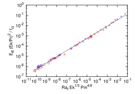
Figure 1: (Color online) $(E_{B}/f_{\Omega})(\mathrm{Ek}/\mathrm{Pr})^{2}$ as a function of $\mathrm{Ra_{f}}\,\mathrm{Pm}^{1/3}$ (top panel) and $\mathrm{Ra_{f}}\,\mathrm{Ek}^{1/3}\,\mathrm{Pm}^{4/9}$ (bottom panel). Results for $Pm=1$ are shown in blue and those for $Pm=3$ are in red. For $Pm=1$, the Ekman numbers of $2\times 10^{-4}$, $2\times 10^{-5}$, and $2\times 10^{-6}$ are indicated by the plus sign, triangle down, and circle, respectively, whereas for $Pm=3$, the same Ekman numbers are indicated by the x sign, triangle up, and square. The straight lines show power laws with the exponents 2/3 (top panel) and 3/5 (bottom panel).

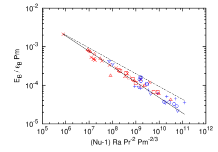
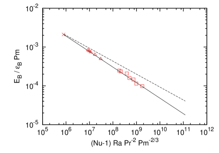
Figure 2: (Color online) $(E_{B}/\epsilon_{B})\mathrm{Pm}$ as a function of $\mathrm{Ra}\,(\mathrm{Nu}-1)\,\mathrm{Pr}^{-2}\,\mathrm{Pm}^{-2/3}$ with the same symbols as in fig. 1. The straight lines indicate power laws with the exponents $-2/5$ (solid line) and $-1/3$ (dashed line). The bottom panel contains the same data as the top panel but shows only points below the transition with $\mathrm{Rm}\,\mathrm{Ek}^{1/3}<13.5$ and $\mathrm{Pm}=3$.

It would be interesting to know a relation between the saturation magnetic field strength and $\mathrm{Ra_{f}}$. From their simulations in spherical shells, Christensen and Aubert Christensen and Aubert (2006) find $(E_{B}/f_{\Omega})(\mathrm{Ek}/\mathrm{Pr})^{2}=(0.76\,\mathrm{Ra_{f}}^{0.32}\mathrm{Pm}^{0.11})^{2}$ where $f_{\Omega}$ is the ratio of ohmic to total dissipation, which in the units used here is given by

$$f_{\Omega}=\frac{\epsilon_{B}/\mathrm{Pm}}{(\epsilon_{v}+\epsilon_{B}/\mathrm{Pm})}$$ (11)

with

$$\epsilon_{B}=\frac{1}{V}\int<(\nabla\times\bm{B})^{2}>dV$$ (12)

and

$$\epsilon_{v}=\frac{1}{V}\int<(\partial_{j}v_{i})(\partial_{j}v_{i})>dV,$$ (13)

where summation over repeated indices is implied and the integration extends over the whole computational volume. The form of this scaling comes from an attempt to determine the magnetic field strength not from a balance of forces but from energy considerations. One can derive from the equations of evolution (2-6) (in the limit of large sound speed $c$, i.e. in the standard Boussinesq limit) the energy budget

$$\epsilon_{v}+\frac{\epsilon_{B}}{\mathrm{Pm}}=(\mathrm{Nu}-1)\mathrm{Ra}.$$ (14)

For the spherical dynamo models with the radial variation of gravity usually simulated, an exact equation of the same structure is not available, but a fit in ref. Christensen and Aubert (2006) shows that the total dissipation is still approximately proportional to $(\mathrm{Nu}-1)\mathrm{Ra}$. The purely ohmic dissipation is related to the total dissipation by the factor $f_{\Omega}$ by definition, and $E_{B}/\epsilon_{B}$ is the square of a magnetic length scale, $l_{B}$, with

$$l_{B}=\sqrt{E_{B}/\epsilon_{B}}.$$ (15)

The magnetic dissipation time, defined as the ratio of magnetic energy and ohmic dissipation, made nondimensional with the ohmic diffusion time, is also given by $E_{B}/\epsilon_{B}$. Ref. Christensen and Aubert (2006) finds an acceptable fit for $l_{B}$ as a function of the control parameters of the flow, which together with the fit for the total dissipation rate as a function of $(\mathrm{Nu}-1)\mathrm{Ra}$ leads to a relation between $E_{B}/\epsilon_{B}$ and the control parameters. A more elaborate fitting procedure Stelzer and Jackson (2013) in which one searches directly a power law fit for $E_{B}/f_{\Omega}$ as a function of $\mathrm{Ra_{f}}$, $\mathrm{Ek}$ and the Prandtl numbers leads to $(E_{B}/f_{\Omega})(\mathrm{Ek}/\mathrm{Pr})^{2}=(0.60\,\mathrm{Ra_{f}}^{0.31}\mathrm{Pm}^{0.16})^{2}$. For the purpose of the discussion below, we can round the exponents to

$$\frac{E_{B}}{f_{\Omega}}\left(\frac{\mathrm{Ek}}{\mathrm{Pr}}\right)^{2}\propto\left(\mathrm{Ra_{f}}\,\mathrm{Pm}^{1/3}\right)^{2/3}.$$ (16)

The data available for the plane layer will not allow us to determine an exponent for $\mathrm{Pm}$, and the analysis of the $\mathrm{R}a_{f}$ dependence will not depend on discrepancies of 0.01 in the exponent. Note also that the factor $\mathrm{Ek}/\mathrm{Pr}$ on the left hand side is due to the different units of magnetic field used here and in ref. Christensen and Aubert, 2006. Eq. (16) has no predictive power for $E_{B}$ unless one guesses $f_{\Omega}$. However, an upper bound for $f_{\Omega}$ is 1, resulting in an upper bound for $E_{B}$ if $f_{\Omega}$ is set to 1 in Eq. (16).

Figure 1 shows $(E_{B}/f_{\Omega})(\mathrm{Ek}/\mathrm{Pr})^{2}$ as a function of $\mathrm{Ra_{f}}\,\mathrm{Pm}^{1/3}$ for the plane layer dynamos and eq. (16) seems to provide a satisfying fit. Remarkably, there is no trace of a transition between different types of dynamos in this plot. However, one can simplify Eq. (16) by using the energy budget (14) in order to obtain

$$\frac{E_{B}}{\epsilon_{B}}\mathrm{Pm}\propto\left(\mathrm{Ra}\,(\mathrm{Nu}-1)\,\mathrm{Pr}^{-2}\,\mathrm{Pm}^{-2/3}\right)^{-\alpha}.$$ (17)

with $\alpha=1/3$. This equation is simpler than eq. (16) because common factors $\mathrm{Ra}(\mathrm{Nu}-1)$ and $\mathrm{Ek}$ are removed. Figure 2 shows $(E_{B}/\epsilon_{B})\mathrm{Pm}$ as a function of $\mathrm{Ra}(\mathrm{Nu}-1)\mathrm{Pr}^{-2}\mathrm{Pm}^{-2/3}$. Because of the removal of the common factors, the data points spread over fewer decades and it becomes apparent that $\alpha=1/3$ is not an acceptable exponent, neither as a fit to the data cloud as a whole, nor to the points below the transition at $\mathrm{Rm}\,\mathrm{Ek}^{1/3}=13.5$, nor to individual series of simulations at $\mathrm{Ek}$, $\mathrm{Pm}$ and $\mathrm{Pr}$ constant. Instead, the best fitting exponent is close to $\alpha=2/5$. This exponent describes the dependence on $\mathrm{Ra}(\mathrm{Nu}-1)$. The dependence on $\mathrm{Pm}$ and $\mathrm{Pr}$ is not seriously tested by the data.

We can now reinflate eq. (17) for $\alpha=2/5$ with the help of the energy budget to obtain a relation analogous to eq. (16), which becomes

$$\frac{E_{B}}{f_{\Omega}}\left(\frac{\mathrm{Ek}}{\mathrm{Pr}}\right)^{2}=0.55\left(\mathrm{Ra_{f}}\,\mathrm{Ek}^{1/3}\,\mathrm{Pm}^{4/9}\right)^{3/5}.$$ (18)

where the prefactor is taken from fig. 1 which shows eq. (18) to be a satisfactory fit, again. An $\mathrm{Ek}$ dependence of the right hand side therefore appears in eq. (18). In the spherical models on the contrary, the best fit does not contain any $\mathrm{Ek}$ dependence (see table 4 of ref. Stelzer and Jackson, 2013).

For completeness, fig. 3 plots $f_{\Omega}$ as a function of $\mathrm{Rm}\,\mathrm{Ek}^{1/3}$. It is plausible that $f_{\Omega}$ is small for dynamos close to the onset in the case of a supercritical bifurcation and that $f_{\Omega}$ approaches 1 as the magnetic field grows stronger. However, $f_{\Omega}$ is already 0.7 at the smallest $\mathrm{Rm}\,\mathrm{Ek}^{1/3}$ in fig. 3. This supports the scenario of a subcritical convection driven dynamo in plane layers Stellmach and Hansen (2004); Jones and Roberts (2000). According to Tilgner (2012), a second type of dynamo operates for $\mathrm{Rm}\,\mathrm{Ek}^{1/3}>13.5$, and in this range, $f_{\Omega}$ is increasing as a function of $\mathrm{Rm}\,\mathrm{Ek}^{1/3}$ as expected. When scalings of $E_{B}$ are sought in terms of $\mathrm{Rm}$ and $\mathrm{Ek}$, these two types of dynamos have to be considered separately Tilgner (2012), but they can be fitted simultaneously in a graph of $E_{B}/f_{\Omega}$ like fig. 1 because the complications of the transition are hidden in $f_{\Omega}$.

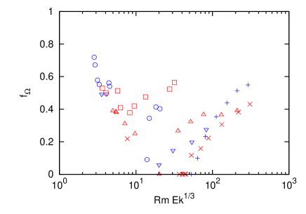
Figure 3: (Color online) $f_{\Omega}$ as a function of $\mathrm{Rm}\,\mathrm{Ek}^{1/3}$ with the same symbols as in fig. 1.

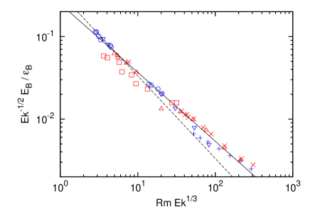
Figure 4: (Color online) $\mathrm{Ek}^{-1/2}E_{B}/\epsilon_{B}$ as a function of $\mathrm{Rm}\,\mathrm{Ek}^{1/3}$ with the same symbols as in fig. 1. The straight lines indicate power laws with the exponents $-5/6$ (solid line) and $-1$ (dashed line).

Figure 5: $\bar{E}/(E_{B}-\bar{E})$ as a function of $\mathrm{Rm}\,\mathrm{Ek}^{1/3}$ for $A=0.5$ (circles), 1 (crosses) and 2 (stars). The dashed line follows the prediction of first order smoothing and shows $\bar{E}/(E_{B}-\bar{E})\propto(\mathrm{Rm}\,\mathrm{Ek}^{1/3})^{-2}$. The solid lines plot the functions $0.09/\sqrt{x}$, $0.09/(4\sqrt{x})$, and $0.09/(16\sqrt{x})$.

The magnetic length scale $l_{B}$ introduced in eq. (15) is connected to the total dissipation $\mathrm{Ra}\,(\mathrm{Nu}-1)$ in Eq. (17). It is more natural to seek a relation between $l_{B}$ and $\mathrm{Rm}$. From spherical shell simulations, ref. Christensen and Tilgner, 2004 infers $E_{B}/\epsilon_{B}\propto 1/\mathrm{Rm}$, whereas a more extended analysis Christensen (2004) yielded $E_{B}/\epsilon_{B}\propto\mathrm{Rm}^{-5/6}(\mathrm{Ek}/\mathrm{Pm})^{1/6}$. There is no theoretical basis for this relationship, it is at present a purely empirical finding. Fig. 4 shows $\mathrm{Ek}^{-1/2}E_{B}/\epsilon_{B}$ as a function of $\mathrm{Rm}\,\mathrm{Ek}^{1/3}$ and confirms the dependence of $l_{B}$ on $\mathrm{Rm}$ in $\mathrm{Rm}^{-5/6}$ which is therefore identical in spherical and in planar geometry, and also confirms the $\mathrm{Ek}$ dependence found in ref. Christensen (2004) to within a factor $\mathrm{Ek}^{1/18}$, which is too small to be discerned in the data.

Fig. 4 shows that the behavior of the magnetic dissipation length $l_{B}$ is not affected by the transition at $\mathrm{Rm}\,\mathrm{Ek}^{1/3}=13.5$ and that it behaves the same for the two types of dynamos, above and below the transition. The variable $\mathrm{Rm}\,\mathrm{Ek}^{1/3}$ does on the other hand decide on whether a mean field is generated. The energy in the mean field, $\bar{E}$, is computed as

$$\bar{E}=\frac{1}{2}\frac{1}{V}<\int dz\left(\int dy\int dx\,\bm{B}\right)^{2}>.$$ (19)

It is well known that close to the onset of dynamo action in rapidly rotating plane layer convection, the generated magnetic field is dominated by its mean field component Stellmach and Hansen (2004). The dynamo is then accessible to the tools of mean field magnetohydrodynamics and first order smoothing Soward (1974) which predict $\bar{E}/(E_{B}-\bar{E})\propto(\mathrm{Rm}\,\mathrm{Ek}^{1/3})^{-2}$. In the simulations presented here, the ratio $\bar{E}/(E_{B}-\bar{E})$ was smaller than 0.01 at the highest $\mathrm{Rm}\,\mathrm{Ek}^{1/3}$. The simulations at $\mathrm{Ek}=2\times 10^{-5}$ and $\mathrm{Pm}=3$ have been complemented by simulations at different aspect ratios. Most points have been obtained at an aspect ratio of 0.5, and a few points have been added for aspect ratios 1 and 2. The result is shown in fig. 5. If the aspect ratio is increased for points below the transition at $\mathrm{Rm}\,\mathrm{Ek}^{1/3}<13.5$, one observes variations in both $\mathrm{Rm}$ and $\bar{E}$ which increase as one approaches the transition. However, the variation in $\bar{E}/(E_{B}-\bar{E})$ is always less than by a factor of 2 even if the aspect ratio changes by a factor of 4. Above the transition, on the other hand, an increase of the aspect ratio $A$ by a factor of 2 always reduces $\bar{E}/(E_{B}-\bar{E})$ by a factor of 4. This behavior is readily understood if one assumes that these dynamos do not genuinely generate a mean field, but that the statistical fluctuations of the local field do not cancel exactly in a volume of finite size. Assume that the magnetic field has a correlation length $l_{c}$. The number of independent degrees of freedom in a plane of cross section $A\times A$ is $(A/l_{c})^{2}$. The mean field computed in each plane is the sum of $(A/l_{c})^{2}$ random numbers drawn from a probability distribution with a width proportional to $\sqrt{E_{B}}$, so that $\bar{E}/(E_{B}-\bar{E})\approx\bar{E}/E_{B}\propto(l_{c}/A)^{2}$. Doubling $A$ thus reduces $\bar{E}/(E_{B}-\bar{E})$ by a factor of 4.

The evidence thus points at a dynamo without a mean magnetic field above the transition, even though in any numerical realization, the mean field is not exactly zero but depends on the aspect ratio. Below the transition, the dynamo does generate a mean field, but as its amplitude is small, the contribution from the statistical fluctuations of the mean field introduces some aspect ratio dependence in these dynamos as well.

Favier and Bushby Favier and Bushby (2013) also found in their simulations of dynamos in rotating compressible convection a mean field which decreases with increasing aspect ratio, so that the mean field detected in these simulations may well be a statistical feature as described above. Cattaneo and Hughes Cattaneo and Hughes (2006) simulate dynamos which produce magnetic energy spectra which peak at small scales suggesting a dynamo process at small scales (similarly to Favier and Bushby (2013)). They for example present a case with $\mathrm{Rm}\,\mathrm{Ek}^{1/3}$ around 200 (which is clearly above the transition) at the relatively large $\mathrm{Ek}$ of $2.8\times 10^{-3}$ and an aspect ratio of 10 and find as expected a small value for $E_{B}/\epsilon_{B}$ on the order of $10^{-4}$.

Large mean fields were observed on the other hand in refs. Stellmach and Hansen (2004); Jones and Roberts (2000); Rotvig and Jones (2002). Stellmach and Hansen Stellmach and Hansen (2004) used the exact same model as here, but simulated Rayleigh numbers closer to onset than in the present study, so that the existence of an important mean field is not surprising. Refs. Jones and Roberts (2000); Rotvig and Jones (2002) used Rayleigh numbers a few times and up to ten times critical, and Ekman numbers comparable to these in the present study, so that these dynamos should be examples of dynamos below the transition. The authors found mean fields about 2-3 times as large as here. One may speculate that this is due to different boundary conditions: For the perfectly conducting boundaries used here, the average over $z$ of the mean field must be zero Jones and Roberts (2000), but this constraint does not exist for the insulating boundaries used in refs. Jones and Roberts (2000); Rotvig and Jones (2002).

In summary, convection in rotating plane layers supports dynamos both with and without a mean field. The scaling exponents for the energy and the magnetic dissipation length inferred from simulations in spherical shells at first glance fit perfectly well the data from the plane layer. However, closer inspection reveals the field energy scaling proposed for the spherical shell to be unacceptable for the plane layer data. Of course, more aspects of the model than the boundary geometry have been changed in going from the usual spherical dynamo simulation to the plane layer model presented here, such as the spatial variation of gravity and the magnetic boundary conditions, and it is not yet possible to tell which of those features is relevant for the magnetic field scalings. The present work at any rate leads us to also expect differences between different spherical models, such as models with different ratios of outer and inner radii, with different radial dependencies of gravity, or with different boundary conditions.

References

- Christensen and Aubert (2006) U. Christensen and J. Aubert, Geophys. J. Int., 166, 97 (2006).
- Christensen et al. (2009) U. Christensen, V. Holzwarth, and A. Reiners, Nature, 457, 167 (2009).
- Dwyer et al. (2011) C. Dwyer, D. Stevenson, and F. Nimmo, Nature, 479, 212 (2011).
- Le Bars et al. (2011) M. Le Bars, M. Wieczorek, O. Karatekin, D. Cébron, and M. Laneuville, Nature, 479, 215 (2011).
- Tilgner (2012) A. Tilgner, Phys. Rev. Lett., 109, 248501 (2012).
- Chorin (1967) A. Chorin, J. Comp. Phys., 2, 12 (1967).
- Schmitz and Tilgner (2010) S. Schmitz and A. Tilgner, Geophys. Astrophys. Fluid Dynam., 104, 481 (2010).
- Stelzer and Jackson (2013) Z. Stelzer and A. Jackson, Geophys. J. Int., 193, 1265 (2013).
- Stellmach and Hansen (2004) S. Stellmach and U. Hansen, Phys. Rev. E, 70, 056312 (2004).
- Jones and Roberts (2000) C. Jones and P. Roberts, J. Fluid Mech., 404, 311 (2000).
- Christensen and Tilgner (2004) U. Christensen and A. Tilgner, Nature, 429, 169 (2004).
- Christensen (2004) U. Christensen, Space Science Rev., 152, 565 (2004).
- Soward (1974) A. Soward, Phil. Trans. R. Soc. Lond. A, 275, 611 (1974).
- Favier and Bushby (2013) B. Favier and P. Bushby, J. Fluid Mech., 723, 529 (2013).
- Cattaneo and Hughes (2006) F. Cattaneo and D. Hughes, J. Fluid Mech., 553, 401 (2006).
- Rotvig and Jones (2002) J. Rotvig and C. Jones, Phys. Rev. E, 66, 056308 (2002).