Configurational entropy of hydrogen-disordered ice polymorphs

Abstract

The configurational entropy of several H-disordered ice polymorphs is calculated by means of a thermodynamic integration along a path between a totally H-disordered state and one fulfilling the Bernal-Fowler ice rules. A Monte Carlo procedure based on a simple energy model is used, so that the employed thermodynamic path drives the system from high temperatures to the low-temperature limit. This method turns out to be precise enough to give reliable values for the configurational entropy $s_{th}$ of different ice phases in the thermodynamic limit (number of molecules $N\to\infty$). The precision of the method is checked for the ice model on a two-dimensional square lattice. Results for the configurational entropy are given for H-disordered arrangements on several polymorphs, including ices Ih, Ic, II, III, IV, V, VI, and XII. The highest and lowest entropy values correspond to ices VI and XII, respectively, with a difference of 3.3% between them. The dependence of the entropy on the ice structures has been rationalized by comparing it with structural parameters of the various polymorphs, such as the mean ring size. A particularly good correlation has been found between the configurational entropy and the connective constant derived from self-avoiding walks on the ice networks.

I Introduction

Water presents a large variety of solid phases. Up to now sixteen different crystalline ice polymorphs have been identified, most of them obtained by application of high pressures, which produces a denser packing of water molecules than in the usual hexagonal ice Ih.Petrenko and Whitworth (1999); Dunaeva et al. (2010); Bartels-Rausch et al. (2012) The determination of their crystal structures and stability range in the pressure-temperature phase diagram has been a subject of investigation over the last few decades. However, in spite of the wide amount of experimental and theoretical works on the solid phases of water, some of their properties still lack a full understanding. This is largely due to the presence of hydrogen bonds between adjacent molecules, which give rise to some peculiar characteristics of these condensed phases (the so-called ‘water anomalies’).Eisenberg and Kauzmann (1969); Petrenko and Whitworth (1999); Robinson et al. (1996)

In the known ice polymorphs (leaving out ice X), water molecules appear as well defined entities forming a network linked by H-bonds. In such a network each H₂O molecule is H-bonded to four others in a disposition compatible with the so-called Bernal-Fowler ice rules. These rules state that each molecule is oriented so that its two H atoms point toward adjacent oxygen atoms and that there must be exactly one H atom between two contiguous oxygens.Bernal and Fowler (1933) We will refer to these rules simply as ‘ice rules.’

Orientational disorder of the water molecules is present in several ice phases. Oxygen atoms show full occupancy ($f$) of their crystallographic sites ($f=1$), but hydrogen atoms may present a disordered distribution, as indicated by a fractional occupancy of their lattice positions ($f<1$). For example, hexagonal ice Ih presents full hydrogen disorder compatible with the ice rules (occupancy of H-sites $f=0.5$). Other polymorphs such as ice II are H-ordered, while some phases as ices III and V display partial hydrogen order (some fractional occupancies $f\neq 0.5$).

The sixteen known crystalline ice phases can be classified according to their network topology. Thus, one finds polymorphs sharing the same topology, as happens for ices Ih and XI. Something similar occurs for other ice polymorphs, and at present six such pairs of ice structures are known: Ih-XI, III-IX, V-XIII, VI-XV, VII-VIII, and XII-XIV,Salzmann et al. (2011) where the first polymorph in each pair is H-disordered and the second is H-ordered. In each case, both polymorphs share the same network topology and are related one to the other through an order/disorder phase transition. In addition to these twelve polymorphs, there exist other ice structures for which no pair has been found: ice Ic (H-disordered), ice II (H-ordered), and ice IV (H-disordered). Finally, ice X is topologically equivalent to ices VII and VIII, with the main difference that in ice X hydrogen atoms are situated on the middle point between adjacent oxygen atoms, so that water molecules lose in fact their own entity. Then, one has nine topologically different ice structures. We note that the ice VII network (as well as ices VIII and X) consists of two independent interpenetrating subnetworks not hydrogen-bonded to each other (each of them equivalent to the ice Ic network). There is another case, the pair VI-XV, for which the network is also made up of two disjoint subnetworks, but they are not equivalent to the network of any other known ice polymorph.

The first evaluation of the configurational entropy $S$ associated to H disorder in ice was presented by Pauling,Pauling (1935) who found $S=Nk_{B}\ln(3/2)$ for a crystal of $N$ water molecules. This result turned out to be in rather good agreement with the ‘residual’ entropy obtained from the experimental heat capacity of ice Ih,Giauque and Stout (1936); Haida et al. (1974) even though the calculation did not consider the actual structure of this ice polymorph. NagleNagle (1966) calculated later the residual entropy of hexagonal ice Ih and cubic ice Ic by a series method, and found for both polymorphs very similar values, which were close to but slightly higher than the Pauling’s estimate. In recent years, Berg et al.Berg et al. (2007, 2012) have employed multicanonical simulations to calculate the configurational entropy of ice Ih, assuming a disordered H distribution consistent with the ice rules. Furthermore, the configurational entropy of partially ordered ice phases has been studied earlier,Howe and Whitworth (1987); MacDowell et al. (2004); Berg and Yang (2007) and will not be addressed here.

Besides their application to condensed phases of water, ice-type models are relevant for other types of solids displaying atomic or spin disorder,Isakov et al. (2004); Pomaranski et al. (2013) as well as in statistical-mechanics studies of lattice problems.Ziman (1979); Bell and Lavis (1989) At present, no analytical solutions for the ice model in actual three-dimensional (3D) ice structures are known, so that no exact values for the configurational entropy are available. An exact solution was found by LiebLieb (1967a, b) for the two-dimensional (2D) square lattice, where the entropy resulted to be $S=Nk_{B}\ln W$, with $W=(4/3)^{3/2}=1.5396$, a value somewhat higher than Pauling’s result $W_{P}=1.5$.

A goal of the present work consists in finding relations between thermodynamic properties and topological characteristics of ice polymorphs. In this line, it has recently been shown that the network topology plays a role to quantitatively describe the configurational entropy associated to hydrogen disorder in ice structures.Herrero and Ramírez (2013a) This has been known after the work by Nagle,Nagle (1966) who showed that the actual structure is relevant for this purpose, by comparing his results for ices Ih and Ic with Pauling’s value for the configurational entropy, which is in fact the limiting value corresponding to a loop-free network (Bethe lattice).

In this paper, we present a simple but ‘formally exact’ numerical method, to obtain the configurational entropy of H-disordered ice structures. It is based on a thermodynamic integration from high to low temperatures for a model whose lowest-energy states are consistent with the ice rules. The configurational space is sampled by means of Monte Carlo (MC) simulations, which provide us with accurate values for the heat capacity of the considered model. This method has been employed earlier to calculate the entropy of H-disordered ices Ih and VI in Ref. Herrero and Ramírez, 2013a. Apart from ice Ih, Ic, and VI, we are not aware of any calculation of the configurational entropy of other H-disordered ice polymorphs. Entropy calculations have been also carried out earlier for H distributions displaying partial ordering on the available crystallographic sites, as happens for ices III and V.MacDowell et al. (2004)

II Method of calculation

For concreteness, we recall the ice rules, as established by Bernal and FowlerBernal and Fowler (1933) in 1933: First, there is one hydrogen atom between each pair of neighboring oxygen atoms, forming a hydrogen bond, and second, each oxygen atom is surrounded by four H atoms, two of them covalently bonded and two other H-bonded to it. Fulfillment of these rules implies that short-range order must be present in the distribution of H atoms in ice polymorphs.

Calculating the configurational entropy of different ice structures, assuming that the hydrogen distribution is only conditioned by the ice rules, is equivalent to find the number of possible hydrogen configurations compatible with these rules. Since the entropy is a state function, one can employ any thermodynamic integration that connects the required state with any other state whose thermodynamic properties are known. For the present problem, this can be adequately done by considering a simple model, in which an energy function is defined so that all states compatible with the ice rules are equally probable (have the same energy $U_{0}$), and other hydrogen configurations have higher energy. The calculation of the configurational entropy of ice is thus reduced to finding the degeneracy of the ground state of considered model. Taking the H configurations according to their Boltzmann weight, as is usual in the canonical ensemble, only those with the minimum energy $U_{0}$ will appear for $T\to 0$. In this respect, the only requirement for a valid energy model is that it has to reproduce the ice rules at low temperature. Thus, irrespective of its simplicity, it will yield the actual configurational entropy if an adequate thermodynamic integration is carried out.

Our model is defined as follows. We consider an ice structure as defined by the positions of the oxygen atoms, so that each O atom has four nearest O atoms. This defines a network, where the nodes are the O sites, and the links are H-bonds between nearest neighbors. The network coordination is four, which gives a total of $2N$ links, $N$ being the number of nodes. We assume that on each link there is one H atom, which can move between two positions on the link (close to one oxygen or close to the other). We will use reduced variables, so that quantities such as the energy $U$ and the temperature $T$ are dimensionless. The entropy per site $s$ presented below is related with the physical configurational entropy $S$ as $S=Nk_{B}s$, $k_{B}$ being Boltzmann’s constant.

Figure 1: Schematic illustration of the different hydrogen configurations around an oxygen atom. Open and solid circles represent oxygen and hydrogen atoms, respectively. For each configuration, $i$ is the number of H atoms close (covalently bonded) to the central oxygen, $g(i)$ indicates its multiplicity, and $E(i)$ is its dimensionless energy in the model described in the text.

For a given configuration of H atoms on an ice network, the energy $U$ is defined as:

$$U=\sum_{n=1}^{N}E(i_{n})$$ (1)

where the sum runs over the $N$ nodes in the network, and $i_{n}$ is the number of hydrogen atoms covalently bonded to the oxygen on site $n$, which can take the values $i_{n}$ = 0, 1, 2, 3, or 4. The energy associated to site $n$ is defined as $E(i_{n})=|i_{n}-2|$ (see Fig. 1), having a minimum for $i_{n}=2$ ($E_{2}=0$), which imposes accomplishment of the ice rules at low temperature. In this way, all hydrogen configurations compatible with the ice rules on a given structure are equally probable, because they have the same energy ($U_{0}=0$ in our case).

This energy model is a convenient tool to derive the configurational entropy, but it does not represent any realistic interatomic interaction. In fact, we are not dealing with an actual ordering process in an H-bond network, but with a numerical approach to ‘count’ H-disordered configurations. One can obtain the number of configurations compatible with the ice rules on a given structure by a thermodynamic integration, going from a reference state ($T\to\infty$) for which the H configuration is random (does not follow the ice rules), to a state in which these rules are strictly satisfied ($T\to 0$).

This model assumes that all hydrogen arrangements that satisfy the Bernal-Fowler rules are energetically degenerate. In the actual ice structures there will be variations in the energy due to different hydrogen bonding patterns.Knight et al. (2006); Singer and Knight (2012) For large system size and at temperatures at which the H-disordered phases are stable, the crystal structures corresponding to different hydrogen arrangements will form a nearly degenerate energy band, populated almost uniformly. Thus, the idea underlying the calculation of ‘residual’ entropies is that the accessible hydrogen configurations do not correspond to the actual stable phase at $T=0$ (which should be ordered), but to an equilibrium H-disordered phase at higher $T$. This means that small energy differences between different hydrogen arrangements are supposed to not affect significantly their relative weight for the residual entropy, as these arrangements will have nearly the same probability in the (equilibrium) disordered phase.

We obtain the configurational entropy per site at temperature $T$ from the heat capacity, $c_{v}$, as

$$s(T)=s(\infty)+\int_{\infty}^{T}\frac{c_{v}(T^{\prime})}{T^{\prime}}\,d\,T^{\prime}$$ (2)

where

$$c_{v}(T)=\frac{1}{N}\frac{d\langle U\rangle}{d\,T}\,,$$ (3)

and the entropy in the high-temperature limit ($T\to\infty$) is given by

$$s(\infty)=\frac{1}{N}\ln(2^{2N})=2\ln 2$$ (4)

Here, $2N$ is the number of links in the considered network, and $2^{2N}$ is the total number of possible configurations in our model, as two different positions are accessible for an H atom on each link.

Although Eq. (2) is exact in principle, a practical problem in this thermodynamic integration appears because the limit $T\to\infty$ cannot be reached in actual simulations. One can introduce a high-temperature cutoff $T_{c}$ for this integration, but even if $T_{c}$ is very high (in our units $T_{c}\gg 1$), it may introduce uncontrolled errors in the calculated entropies. Thus, a reasonable solution to this problem can be calculating the integral in Eq. (2) up to a temperature $T_{c}$, and then obtaining the remaining part (from $T_{c}$ to $T=\infty$) by an alternative method. With this purpose, an analytical procedure has been introduced in Ref. Herrero and Ramírez, 2013a, and is described in the following section dealing with an independent-site model.

II.1 Independent-site model

For a real ice network, thermodynamic variables at high temperatures ($T\gg 1$ here) can be well described by considering ‘independent’ nodes, as in Pauling’s original calculation for a hypothetical loop-free network. In such a case, the partition function can be written as

$$Z=\frac{z^{N}}{2^{2N}}\,,$$ (5)

$z$ being the one-site partition function, and the term $2^{2N}$ in the denominator appears to avoid counting links with zero or two H atoms. This correction is in fact similar to that introduced by Pauling in his entropy calculation.Pauling (1935)

To obtain the partition function $z$, we consider the 16 possible configurations of four hydrogen atoms, as given in Fig. 1, which yields at temperature $T$:

$$z=\sum_{i=0}^{4}g(i)\,\exp\left[-\frac{E(i)}{T}\right]=6+8\,{\rm e}^{-1/T}+2\,{\rm e}^{-2/T}\,.$$ (6)

From this expression for $z$ one obtains the partition function $Z$ using Eq. (5). Thus, the high-temperature limit of $Z$ is $Z_{\infty}=16^{N}/4^{N}=2^{2N}$, which is the number of configurations compatible with the condition of having an H atom per link, as indicated above.

In this independent-site model, the energy per site at temperature $T$ is

$$\langle u\rangle=\frac{1}{N}\,T^{2}\,\frac{\partial\ln Z}{\partial T}=\frac{4}{z}\left(2\,{\rm e}^{-1/T}+{\rm e}^{-2/T}\right)\,.$$ (7)

For the entropy per site we have

$$s=\frac{1}{N}\,\frac{\partial\,(T\ln Z)}{\partial\,T}\,,$$ (8)

and using Eqs. (5) and (7), one finds

$$s=\ln z+\frac{\langle u\rangle}{T}-2\ln 2\,.$$ (9)

In the limit $T\to 0$ (ice rules strictly fulfilled), we have

$$\lim_{T\to 0}\frac{\langle u\rangle}{T}=0\,,$$ (10)

and $z\to 6$ [see Eq.(6)], so that $s(0)=\ln\frac{3}{2}$, which coincides with Pauling’s result.Pauling (1935)

For our calculations on real ice networks we will employ a cutoff temperature $T_{c}=10$. Introducing this temperature in Eq. (9), we find for the independent-site model $s(T_{c})$ = 1.38414, which coincides with the value obtained in Ref. Herrero and Ramírez, 2013a from a series expansion in powers of $1/T$ up to fourth order.

II.2 Actual ice networks

The above independent-site equations are exact for a loop-free network, i.e., the so-called Bethe lattice or Cayley tree.Ziman (1979); Bell and Lavis (1989) For real ice structures, the corresponding networks contain loops, which means that the factorization of the partition function in Eq. (5) is not possible. Nevertheless, at high temperatures thermodynamic variables for the real structures converge to those of the independent-site model, and this is the fact we use to obtain the high-temperature part of our thermodynamic integration.

Thus, for the actual ice networks we calculate the configurational entropy per site for hydrogen-disordered distributions compatible with the ice rules (accomplished in our method for $T\to 0$) as:

$$s(0)=s(T_{c})-\int_{0}^{T_{c}}\frac{c_{v}(T^{\prime})}{T^{\prime}}\,dT^{\prime}$$ (11)

where $s(T_{c})$ = 1.38414 is the value obtained for the independent-site model, and the heat capacity $c_{v}$ is derived from MC simulations for the considered ice polymorph in the temperature range from $T=0$ to $T=T_{c}$ (we will take $T_{c}=10$ here).

Table 1: Crystal system and space group for the ice polymorphs studied in this work, along with the references from where crystallographic data were taken. $N_{max}$ is the number of water molecules in the largest supercell employed here for each ice structure.

Phase	Crystal system	Space group	Ref.	$N_{max}$
Ih	Hexagonal	$P6_{3}$/$mmc$, 194	Peterson and Levy,1957	2880
Ic	Cubic	$Fd\bar{3}m$, 227	König,1944	2744
II	Rhombohedral	$R\bar{3}$, 148	Kamb et al.,1971	2592
III	Tetragonal	$P4_{1}2_{1}2$, 92	Lobban et al.,2000	2592
IV	Rhombohedral	$R\bar{3}c$, 167	Engelhardt and Kamb,1981	2400
V	Monoclinic	$A2/a$, 15	Lobban et al.,2000	2688
VI	Tetragonal	$P4_{2}/nmc$, 137	Kuhs et al.,1984	3430
XII	Tetragonal	$I\bar{4}2d$, 122	Lobban et al.,1998	2400

Using the energy model described above, we carried out MC simulations on ice networks of different sizes. Crystallographic data employed to generate the ice structures are given in Table I, along with the corresponding references from where they were taken. In this Table we also present the size $N_{max}$ of the largest supercells employed for the different ice polymorphs. Details of the simulations are similar to those employed earlier for ices Ih and VI.Herrero and Ramírez (2013a) For the hydrogen distribution on the available sites along the MC simulations, we assumed periodic boundary conditions. Sampling of the configuration space at different temperatures was carried out by the Metropolis update algorithm.Binder and Heermann (2010) For each network we considered 360 temperatures in the range between $T$ = 10 and $T$ = 1, and 200 temperatures in the interval from $T$ = 1 to $T$ = 0.01. For each considered temperature, we carried out $10^{4}$ MC steps for system equilibration, followed by $8\times 10^{6}$ steps for averaging of thermodynamic variables. A MC step included an update of $2N$ (the number of H-bonds) hydrogen positions successively and randomly chosen. Once calculated the heat capacity $c_{v}(T)$ at the considered temperatures, the integral in Eq. (11) was numerically evaluated by using Simpson’s rule. Finite-size scaling was employed to obtain the configurational entropy per site $s_{th}$ corresponding to the thermodynamic limit (extrapolation to infinite size, $N\to\infty$).

Although the heat capacity $c_{v}(T)$ can be obtained from MC simulations by numerical differentiation using directly its definition in Eq. (3), we found more practical to derive it from the energy fluctuations at temperature $T$. Thus, we employed the expressionChandler (1987)

$$c_{v}(T)=\frac{(\Delta U)^{2}}{N\,T^{2}}\,,$$ (12)

where $(\Delta U)^{2}=\langle U^{2}\rangle-\langle U\rangle^{2}$. In particular, using this expression we obtained $c_{v}$ values with smaller statistical noise than employing Eq. (3).

Now a relevant question is whether the high-temperature replacement of real ice structures by the independent-site model introduces any appreciable error in the calculated configurational entropies. We have checked this point in two different ways. First, we have compared for some temperatures higher than $T_{c}$ the energy and heat capacity obtained in the independent-site model with those derived from MC simulations for actual ice structures. Second, we have calculated the configurational entropy obtained with our procedure in the low-$T$ limit for the ice model on a 2D square lattice, for which an exact analytical solution is known.Lieb (1967a) Both procedures indicate that the error of our method is smaller than the error bars associated to the statistical uncertainty of the MC simulations and the error due to the numerical integration of the ratio $c_{v}/T$ in Eq. (11). This is discussed below.

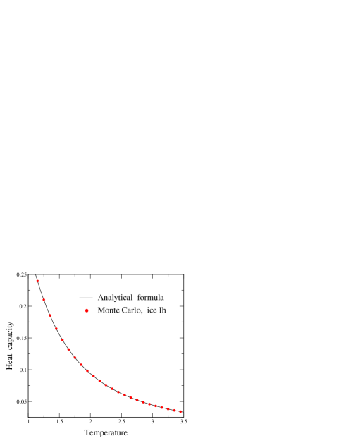
Figure 2: Heat capacity per site as a function of temperature. Solid circles are data points obtained from MC simulations for ice Ih. Error bars are less than the symbol size. The solid line represents the analytical function obtained for the independent-site model as $c_{v}(T)=d\langle u\rangle/dT$ with $\langle u\rangle$ given by Eq. (7).

In Fig. 2 we present the heat capacity $c_{v}(T)$ in the temperature region from $T$ = 1 to 3.5. Symbols are results of our MC simulations for ice Ih, whereas the solid line is the analytical result obtained for the independent-site model as $c_{v}(T)=d\langle u\rangle/dT$, with $\langle u\rangle$ given in Eq. (7). Data obtained by both procedures coincide within the statistical error bars of the simulation results. Although not appreciable in the figure, we observe a trend of the $c_{v}$ values derived from MC simulations to be slightly larger than the analytical ones at temperatures $T\sim 1$. At temperatures $T\sim T_{c}$, differences between both methods are clearly less than the error bars.

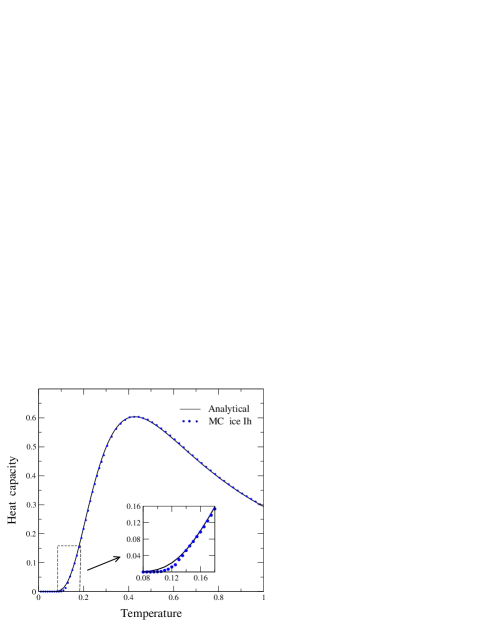
Figure 3: Heat capacity per site as a function of temperature. Solid circles are data points obtained from simulations for the structure of ice Ih. Error bars are less than the symbol size. The solid line corresponds to the independent-site model: $c_{v}(T)=d\langle u\rangle/dT$ with $\langle u\rangle$ given by Eq. (7).

The heat capacity reaches a maximum at $T_{max}\sim 0.4$, and with our numerical precision vanishes at temperatures $T<0.08$. Larger differences between both procedures are observed at temperatures $T<1$, as shown in Fig. 3. At $T\gtrsim 0.4$, results of the MC simulations are slightly larger than the analytical ones, and the opposite happens at $T<0.4$. We observe in the inset that an appreciable difference appears in the region between $T$ = 0.10 and 0.14. Note that the area under the curve $c_{v}(T)$ is independent of the considered network, since it is given by the difference between the high- and low-temperature limits of the energy:

$$\int_{0}^{\infty}c_{v}(T)\,dT=\lim_{T\to\infty}\langle u\rangle-\frac{U_{0}}{N}=0.75$$ (13)

For the energy model considered here we have $U_{0}=0$.

An alternative procedure to calculate the configurational entropy can consist in directly obtaining the density of states as a function of the energy, as described elsewhere for order/disorder problems in condensed-matter problems.Herrero and Ramírez (1992) Thus, the entropy can be obtained in the present problem from the number of states with $U=0$, i.e., compatible with the ice rules.

To avoid any possible misunderstanding, we note that the simple model used in our calculations is not aimed at reproducing any physical characteristic of ice polymorphs (as order/disorder transitions) beyond calculating the entropy of H distributions compatible with the Bernal-Fowler rules. This model implicitly takes for granted that the distribution of H atoms on an ice network does not necessarily display long-range order, and only requires strict fulfillment of the ice rules (short-range order) for $T\to 0$. The configurational entropy derived in this way is what has been traditionally called residual entropy of ice.Pauling (1935) Taking all this into account, we are not allowing for any violation of the third law of Thermodynamics, which implies that for $T\to 0$ an ice polymorph displaying H disorder cannot be the thermodynamically stable phase. Thus, it is generally accepted that the equilibrium ice polymorphs in the low-temperature limit show ordered proton structures, as expected from a vanishing of the entropy. In this context, order-disorder transitions have been observed between several pairs of ice phases.Dunaeva et al. (2010); Bartels-Rausch et al. (2012); Singer and Knight (2012) These transitions are accompanied by an orientational reorganization of water molecules, which turns out to be a kinetically unfavorable rearrangement of the H-bond network.

III Results

We have applied the integration method described above to calculate the configurational entropy of the ice model in eight structures. These structures include the ice polymorphs showing hydrogen disorder, but also the network of ice II, for which no hydrogen disorder has been observed. In this case, the results presented below have to be understood to apply to a hypothetical structure with the same topology as ice II. Moreover, for ices III and V, a partial hydrogen disorder has been found (site occupancies $f$ different from 0.5), a question that will not be taken into account here (see the discussion below on this question). Ice VII will not be discussed, since it consists of two sub-networks, each of them equivalent to the ice Ic network (see the Introduction).

For each considered network, we obtained the configurational entropy $s_{N}$ in the limit $T\to 0$ for several supercells of size $N$, as described in Sect. II. Then, the entropy per site in the thermodynamic limit, $s_{th}$, is obtained by extrapolating $N\to\infty$. The precision of our procedure can be checked by calculating the configurational entropy for the ice model on a 2D square lattice, for which an exact analytical solution is known.Lieb (1967a, b)

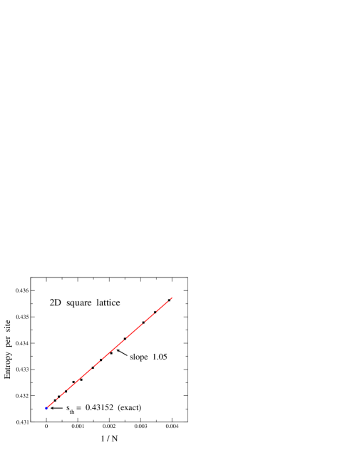
Figure 4: Entropy per site $s_{N}$ vs inverse lattice size ($1/N$) for the 2D square lattice. Solid squares indicate results of our thermodynamic integration in the limit $T\to 0$. Error bars are in the order of the symbol size. A solid circle shows the exact analytical result obtained by Lieb in the limit $N\to\infty$.Lieb (1967a)

In Fig. 4 we present $s_{N}$ for the 2D square lattice as a function of the inverse supercell size $1/N$. Solid squares represent the entropy values yielded by our thermodynamic integration. It is found that the entropy per site $s_{N}$ decreases for increasing size $N$, and a linear dependence of $s_{N}$ on $1/N$ is observed for $N\gtrsim 150$, as

$$s_{N}=s_{th}+\frac{\alpha}{N}\,,$$ (14)

with a slope $\alpha=1.05$. For supercell sizes $N<150$ (not displayed in Fig. 4), $s_{N}$ values slightly deviate from the linear trend given in Eq. (14), being smaller than those predicted from the fit for $N>150$. Extrapolating $s_{N}$ to infinite size ($1/N\to 0$) gives a value $s_{th}$ = 0.43153(3), in agreement with the exact solution for the square lattice derived by LiebLieb (1967a) from a transfer-matrix method: $s_{th}=\frac{3}{2}\ln(4/3)=0.43152$.

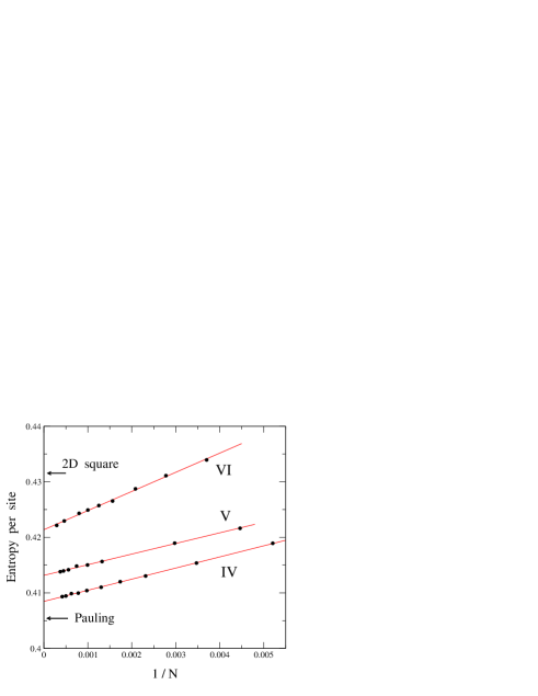
Figure 5: Entropy per site $s_{N}$ as a function of the inverse supercell size ($1/N$) for three ice structures: IV, V, and VI. Data points were derived from thermodynamic integration in the limit $T\to 0$. Error bars are less than the symbol size. Arrows indicate the entropy $s_{th}$ corresponding to the 2D square lattice and the Pauling result.

For the 3D structures of ice polymorphs we also found a linear dependence of the configurational entropy $s_{N}$ on the inverse supercell size. This is shown in Fig. 5 for ices IV, V, and VI. One observes that both the slope $\alpha$ and the infinite-size limit $s_{th}$ depend on the ice structure. The slope is clearly larger than in the 2D case ($\alpha=1.05$), as for ices IV, V, and VI we find $\alpha$ = 2.00(2), 1.91(3), and 3.44(6), respectively. For comparison, arrows in Fig. 5 indicate the entropy per site for the 2D square lattice and the Pauling result. The data for the ice polymorphs converge in the infinite-size limit to $s_{th}$ between those two values.

Table 2: Configurational entropy $s_{th}$ associated to hydrogen disorder in several ice polymorphs, as derived from our Monte Carlo simulations. For comparison we also give results for the 2D square lattice, as well as Pauling’s value (Bethe lattice). $W=\exp(s_{th})$; $n_{p}$: number of data points employed in the linear fits; $\alpha$: slope of the linear fit as in Eq. (14); $\rho$: correlation coefficient.

Ice	$n_{p}$	$\alpha$	$s_{th}$	$W$	$\rho$
Ih	9	1.84(2)	0.41069(8)	1.50786(12)	0.9994
Ic	10	1.82(2)	0.41064(7)	1.50778(11)	0.9994
II	12	1.87(1)	0.40919(4)	1.50560(6)	0.9998
III	12	1.79(2)	0.41165(7)	1.50931(11)	0.9990
IV	10	2.00(2)	0.40847(4)	1.50451(6)	0.9997
V	8	1.91(3)	0.41316(6)	1.51159(9)	0.9992
VI	9	3.44(6)	0.42138(11)	1.52406(16)	0.9990
XII	10	2.08(3)	0.40813(5)	1.50400(8)	0.9992
Square	12	1.05(1)	0.43153(3)	1.53961(5)	0.9994
Pauling	-	-	0.405465	1.5	-

For other ice structures not shown in Fig. 5 we also obtained $s_{th}$ values between the square lattice and the Pauling result (see Table II). The largest value corresponds to ice VI ($s_{th}=0.42138(11)$), and the smallest one was found for ice XII ($s_{th}=0.40813(5)$). Between both values one finds a relative difference of about 3%. For hexagonal ice Ih, the configurational entropy is found to be an 1.3% larger than Pauling’s estimate. For other ice polymorphs, the difference between $s_{th}$ and the Pauling result ranges from 0.7% for ice XII to 3.9% for ice VI.

Information on the least-square fit of $s_{N}$ values for different ice polymorphs, such as the parameter $\alpha$, the correlation coefficient $\rho$, and the number of points $n_{p}$ employed in the fit, are given in Table II. When discussing the configurational entropy of ice, it is usually given in the literature the parameter $W$, instead of the entropy $s_{th}$ itself. Here, we find directly $s_{th}$ from thermodynamic integration and finite-size scaling, so that $W$ values given in Table II were calculated for the different ice polymorphs as $W=\exp(s_{th})$. The error bars $\Delta W$ and $\Delta s_{th}$ for the values of $s_{th}$ and $W$ are related by the expression $\Delta W=W\,\Delta s_{th}$, as can be derived by differentiating the exponential function. Error bars for $s_{th}$ represent one standard deviation, as given by the least-square procedure employed to fit the data. These error bars are less than $\pm 10^{-4}$, except for ice VI, for which we found $\Delta s_{th}=1.1\times 10^{-4}$.

For comparison with the results found for the ice structures, we also give in Table II data for the 2D square lattice (linear fit shown in Fig. 4) and for a loop-free network with coordination $z=4$ (Pauling’s result). Note that, although the result obtained by Pauling was intended to reproduce the residual entropy of ice Ih, it does not take into account the actual ice network, but only the fourfold coordination of the structure.

Now the question arises why the entropy per site decreases for increasing supercell size. A qualitative explanation is the following. Let us call $\Omega_{N}$ the number of configurations compatible with the ice rules for supercell size $N$. For two independent cells of size $N$, the number of possible configurations is then $\Omega_{N}^{2}$. If one puts both cells together to form a larger cell of size $2N$, one has $\Omega_{2N}<\Omega_{N}^{2}$, since configurations not fitting correctly at the border between both $N$-size cells are unsuitable and have to be rejected. Then, one has

$$s_{2N}=\frac{1}{2N}\,\ln\Omega_{2N}<\frac{1}{2N}\,\ln\Omega_{N}^{2}=\frac{1}{N}\,\ln\Omega_{N}=s_{N}$$ (15)

Something similar can be argued in general for two different cell sizes, $N<M$, so that $s_{M}<s_{N}$. This means that the decrease in $s_{N}$ for rising $N$ can be considered to be a consequence of the cyclic boundary conditions. Assuming that $s_{N}$ behaves regularly as a function of $1/N$ in the thermodynamic limit ($1/N\to 0$), one can write for large $N$ the power expansion: $s_{N}=s_{th}+\alpha/N+\beta/N^{2}+...$. In fact, this is what we found from our simulations for the different ice polymorphs, with the parameter $\beta$ so small that a linear dependence of $s_{N}$ on $1/N$ is consistent with the results of the thermodynamic integration at least for $N>150$.

For ice Ih we find $s_{th}$ = 0.41069(8). As already observed in the analytical result by NagleNagle (1966) and in the multicanonical simulations by Berg et al.,Berg et al. (2007, 2012) the configurational entropy is higher than the earlier estimate by Pauling. Our result is somewhat higher than that of Nagle,Nagle (1966) who found $s_{th}$ = 0.41002(10), and slightly higher than the results of multicanonical simulations, although the latter may be compatible with our data, taking into account the error bars. We do not find at present a clear reason why our result for ice Ih is higher than that found by Nagle using a series method. The error bar given by this author is not statistical, and one could argue that maybe it was underestimated, but this question should be further investigated. A discussion on the various results for ice Ih is given in Ref. Herrero and Ramírez, 2013a.

For cubic ice Ic, we found $s_{th}$ = 0.41064(7), which coincides within error bars with our result for hexagonal ice Ih. To our knowledge, the only earlier calculation for ice Ic is that presented by Nagle in 1966,Nagle (1966) who concluded that within the limits of his estimated error, the entropy is the same for ices Ic and Ih, i.e., $s_{th}$ = 0.41002(10). We reach the same conclusion concerning both ice polymorphs, but in our case the entropy value is higher by an 0.15%. This difference seems to be small, but it is significant as it amounts to more than eight times our error bar (standard deviation).

It is known that ices III and V show partially ordered hydrogen distributions. This means that some fractional occupancies of H-sites are different from 0.5. Then, the actual configurational entropy for these polymorphs is lower than that corresponding to a H-disordered distribution compatible with the ice rules. MacDowell et al.MacDowell et al. (2004) calculated the configurational entropy of partially ordered ice phases by using an analytical procedure, based on a combinatorial calculation. For ices III and V, these authors found entropy values $s_{th}$ = 0.3686 and 0.3817, respectively, which they used to calculate the phase diagram of water with the TIP4P model potential. Taking the Pauling result as the entropy value for H-disordered ice phases, the data by MacDowell et al. mean an entropy reduction of 9.1% and 5.9%, for ice III and V, respectively. This is an appreciable entropy reduction, which is noticeable in the calculated phase diagram.MacDowell et al. (2004) However, if one takes for the H-disordered phases more realistic entropy values, as those derived here, the entropy drop due to partial hydrogen ordering is somewhat larger. In fact, one finds 10.5% for ice III and 7.6% for ice V. In any case, it is known that the hydrogen occupancies of the different crystallographic sites may change to some extent with the temperature, so that the configurational entropy will also change.MacDowell et al. (2004)

IV Relation with structural properties

Topological characteristics of solids at the atomic or molecular level have been considered along the years to study properties of various types of materials.Pearson (1972); Liebau (1985); Wells (1986) For crystalline ice polymorphs, a discussion of different network topologies and the relation of ring sizes in the various phases with the crystal volume was presented by Salzmann et al.Salzmann et al. (2011), and more recently by the present authors in Ref. Herrero and Ramírez, 2013b. As indicated earlier,Herrero and Ramírez (2013a) one expects that structural and topological aspects of ice networks can be relevant to understand quantitatively the configurational entropy of H-disordered structures. In particular, this entropy should in some way be related with effective parameters describing topological aspects of the corresponding networks.

Table 3: Minimum ($L_{min}$), maximum ($L_{max}$), and mean ring size $\langle L\rangle$ for different ice structures, along with the corresponding parameter $a$ and connective constant $\mu$. $a$ is the coefficient of the quadratic term in the coordination sequence, $M_{k}\sim ak^{2}$, as in Eq. (16).

Network	$L_{min}$	$L_{max}$	$\langle L\rangle$	$a$	$\mu$
Ih	6	6	6	2.62	2.8793
Ic	6	6	6	2.50	2.8792
II	6	10	8.52	3.50	2.9049
III	5	8	6.67	3.24	2.8714
IV	6	10	9.04	4.12	2.9162
V	4	12	8.36	3.86	2.8596
VI	4	8	6.57	2.00	2.7706
XII	7	8	7.6	4.26	2.9179
Square	4	4	4	0.0	2.6382
Bethe	–	–	–	–	3.0000

The tendency of the entropy $s_{th}$ to increase due to the presence of loops in the ice structures has been pointed out recently.Herrero and Ramírez (2013a) The Pauling approximation ignores the presence of loops, as happens in the Bethe lattice,Ziman (1979); Bell and Lavis (1989) and yields a value $s_{th}=0.40547$. For ice Ih, which contains six-membered rings of water molecules, the configurational entropy is higher than Pauling’s value by an 1.3%, and it is still higher for the ice model on a 2D square lattice, including four-membered rings (a 6.4% with respect to the Pauling approach). For other ice polymorphs with larger ring sizes, one can expect a smaller configurational entropy for disordered hydrogen distributions, and thus closer to the Pauling result. In Table III we give the minimum ($L_{min}$), maximum ($L_{max}$), and mean ring size $\langle L\rangle$ for the ice structures considered here.

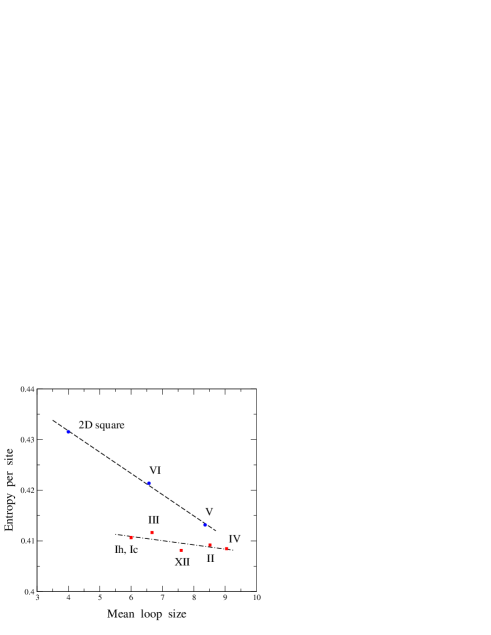
Figure 6: Configurational entropy per site $s_{th}$ vs mean loop size $\langle L\rangle$ for several ice structures. Error bars for the entropy are less than the symbol size. The 2D square lattice is included for comparison. The dashed line is a least-square linear fit to the data of structures containing four-membered rings ($L_{min}=4$). The dashed-dotted line is a fit for the ice structures with $L_{min}>5$.

In this line, we consider the mean loop size $\langle L\rangle$ as a first topological candidate to be compared with $s_{th}$. A correlation between both quantities was suggested in Ref. Herrero and Ramírez, 2013a, and will be considered in more detail here. In Fig. 6 we present the configurational entropy of various ice polymorphs vs $\langle L\rangle$. For comparison, we also include a data point for the 2D square lattice, where all loops have $L=4$. There appears a tendency of the configurational entropy $s_{th}$ to decrease for rising $\langle L\rangle$, but one observes a large dispersion of the data points for different ice polymorphs, indicating a low correlation between both quantities. However, a careful observation of the data displayed in Fig. 6 reveals that points corresponding to the ice structures are roughly aligned, with the exception of ices V and VI, which are located away from the general trend. A common characteristic of these two ice polymorphs is that they contain four-membered rings ($L_{min}=4$). In fact, we find a good linear correlation between $s_{th}$ and the mean ring size $\langle L\rangle$ for these structures and the 2D square lattice (dashed line in Fig. 6). The dashed-dotted line is a linear fit to the data points of ice structures not including four-membered rings. For these structures we have $L_{min}>4$, i.e. $L_{min}=5$ for ice III, $L_{min}=6$ for ices Ih, Ic, II, and IV, and $L_{min}=7$ for ice XII. We observe that the point corresponding to ice III appears above the dashed-dotted line, whereas that corresponding to ice XII lies below it. This appears to be in line with the trend found for ices V and VI, since $L_{min}({\rm III})<6<L_{min}({\rm XII})$, indicating that for a given value of $\langle L\rangle$, a lower $L_{min}$ causes a larger entropy $s_{th}$.

These observations allow us to conclude that the configurational entropy tends to lower as the mean ring size increases, but the presence of four-membered rings greatly affects the actual value of the entropy $s_{th}$. Thus, the configurational entropy for ice VI turns out to be clearly higher than that of ice III, even though both polymorphs have similar values of $\langle L\rangle$. However, the effect of four-membered rings is smaller for larger $\langle L\rangle$, as can be seen by comparing $s_{th}$ values for ices II an V (see Fig. 6).

Further than structural rings, the topology of a given ice network can be characterized by the so-called coordination sequences $\{M_{k}\}$ ($k$ = 1, 2, …), where $M_{k}$ is the number of sites at a topological distance $k$ from a reference site (we call topological distance between two sites the number of bonds in the shortest path connecting one site to the other).Herrero and Ramírez (2013b) For 3D structures, $M_{k}$ increases at large distances as:

$$M_{k}\sim a\,k^{2}\hskip 8.53581pt,$$ (16)

where $a$ is a network-dependent parameter. $M_{k}$ increases quadratically with $k$ just as the surface of a sphere increases quadratically with its radius. For structures including topologically non-equivalent sites, the actual coordination sequences corresponding to different sites may be different, but the coefficient $a$ coincides for all sites in a given structure.Herrero and Ramírez (2013b) This parameter $a$ can be used to define a ‘topological density’ $\rho_{t}$ for ice polymorphs as $\rho_{t}=w\,a$, where $w$ is the number of disconnected subnetworks in the considered network. Usually $w=1$, but for ice structures including two interpenetrating networks (as ices VI and VII) one has $w=2$. The parameter $a$ and the topological density $\rho_{t}$ of crystalline ice structures have been calculated earlier.Herrero and Ramírez (2013b) It was found that $a$ ranges from 2.00 (ice VI) to 4.27 (ice XII), as can be seen in Table III for the ice polymorphs studied here.

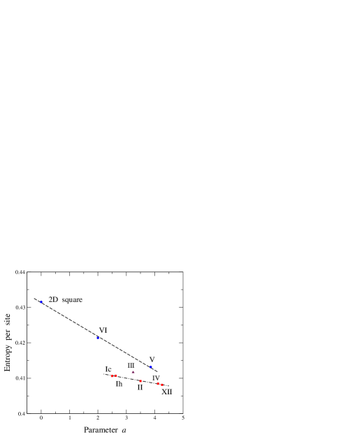
Figure 7: Configurational entropy per site $s_{th}$ vs parameter $a$ of coordination sequences for several ice structures. Error bars for the entropy are less than the symbol size. A point for the 2D square lattice ($a=0$) is shown for comparison. The dashed line is a least-square linear fit to the data of structures containing four-membered rings ($L_{min}=4$). The dashed-dotted line is a fit for the ice structures with $L_{min}>5$.

In Fig. 7 we display the configurational entropy per site $s_{th}$ of ice polymorphs vs the coefficient $a$ derived from the corresponding coordination sequences. We include also a point for the 2D square lattice, for which $a=0$, as in this case the dependence of $M_{k}$ on the distance $k$ is linear: $M_{k}=4k$. We find that $s_{th}$ decreases for increasing parameter $a$, but there appears an appreciable dispersion in the data points, which can be associated to the size of structural rings in the considered ice polymorphs. In particular, ice networks including four-membered rings ($L_{min}=4$) depart clearly from the general trend for the other structures, similarly to the fact observed above in Fig. 6 for the relation between entropy and mean loop size. Thus, two different fits are also displayed in Fig. 7. The dashed line is a linear fit for the ice polymorphs with $L_{min}=4$ (ices V and VI), along with the 2D square lattice. The dashed-dotted line is a least-square linear fit for the structures with $L_{min}>5$, with all of them having $L_{min}=6$ except ice XII, for which $L_{min}=7$. There remains ice III ($L_{min}=5$), not included in either of the fittings, whose data point (solid triangle) lies on the region between both lines in Fig. 7.

From these results we conclude that the configurational entropy tends to decrease as the parameter $a$ (density of nodes) increases. However, the presence of small rings in the ice structures strongly affects the actual value of $s_{th}$. Thus, $s_{th}$ for ices V and VI (with $L_{min}=4$) is clearly larger than that corresponding to ice polymorphs with similar $a$ values but with $L_{min}>4$.

We see that the correlation of the configurational entropy with both the mean loop size and the topological parameter $a$ is highly affected by the presence of structural rings with small number of water molecules, in particular by those of the smallest size found for the known crystalline polymorphs, $L=4$. It would be desirable to find other structural or topological characteristics which could correlate more directly with the entropy $s_{th}$. In this line, various parameters defined in statistical-mechanics studies of lattice problems have been found earlier to be useful to characterize several thermodynamic properties. One of these parameters, which can be used to characterize the topology of ice structures, is the ‘connective constant’ $\mu$, or effective coordination number.Domb (1970); Herrero (1995, 2014) This network-dependent parameter can be calculated from the long-distance behavior of the number of possible self-avoiding walks (SAWs) in the corresponding structures.Binder and Heermann (2010); McKenzie (1976); Rapaport (1985)

A self-avoiding walk on an ice network is defined as a walk in the simplified structure (only oxygen sites, see Sect. II) which can never intersect itself. The number $C_{n}$ of possible SAWs of length $n$ starting from a given network site is asymptotically given byPrivman et al. (1991); McKenzie (1976); Rapaport (1985)

$$C_{n}\sim n^{\gamma-1}\mu^{n}\hskip 5.69054pt,$$ (17)

where $\gamma$ is a critical exponent which takes a value $\approx 7/6$ for 3D structures.McKenzie (1976); Caracciolo et al. (1998); Chen and Lin (2002) Then, the connective constant $\mu$ can be obtained as the limit

$$\mu=\lim_{n\to\infty}\frac{C_{n}}{C_{n-1}}\,.$$ (18)

This parameter $\mu$ depends upon the particular topology of each structure, and has been accurately determined for standard 3D lattices.McKenzie (1976) For the networks of different ice polymorphs, the connective constant $\mu$ has been recently calculated, and was compared with other topological characteristics of these networks.Herrero (2014) It ranges from 2.770 for ice VI to 2.918 for ice XII, as shown in Table III.

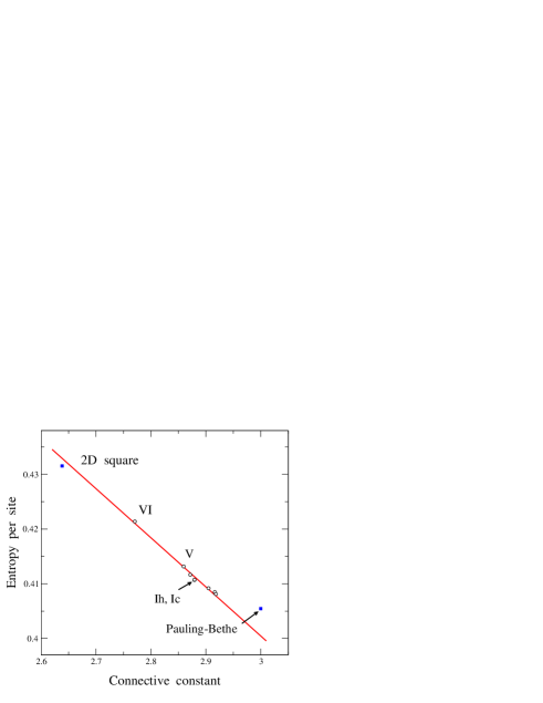
Figure 8: Configurational entropy per site $s_{th}$ vs connective constant $\mu$ for several ice structures (open circles). Values for the 2D square lattice and the Bethe lattice (Pauling model) are displayed for comparison (solid squares). The solid line is a least-square linear fit to the data of ice structures. Error bars for the entropy are less than the symbol size.

In Fig. 8 we present the configurational entropy per site $s_{th}$ vs the connective constant $\mu$ for the considered ice polymorphs, as well as for the loop-free Bethe lattice (Pauling’s result) and the 2D square lattice. One observes in this figure a negative correlation between the entropy $s_{th}$ and $\mu$. The line is a least-square fit to the data points of the ice polymorphs. Data corresponding to the square lattice and the Bethe lattice were not included in the fit, as they depart from the trend of the ice structures. This seems to be due to the role played by dimensionality in the actual values of the configurational entropy (the Bethe lattice has no well-defined dimension $d$, and for some purposes it can be considered as $d\to\infty$).

In relation to the data displayed in Fig. 8 for ice polymorphs, we cannot find at present any reason why the correlation between $s_{th}$ and $\mu$ should be strictly linear, but it is clear that there is a relation between both magnitudes. To obtain some insight into this question, a qualitative argument is the following. The connective constant $\mu$ is a measure of the mean number of sites connected to a node in long SAWs. Then, for the distribution of H atoms on the links of the ice structures according to the Bernal-Fowler rules, a larger $\mu$ is associated to a rise in the correlations between occupancies of different hydrogen sites, as information on the actual occupancy of a link propagates ‘more effectively’ through the ice network.Herrero (2002); Herrero and Saboyá (2003) This correlation gives rise to a decrease in the number of configurations compatible with the ice rules for a given structure, which means a reduction of the configurational entropy of the hydrogen distribution on the considered ice network. Similar relations between SAWs and order/disorder problems, such as Ising or lattice-gas models, have been found and discussed earlier.Pelissetto and Vicari (2002); Domb (1970); Herrero (1995) In this line, the relation observed here between configurational entropy and SAWs should be investigated further in the context of the statistical mechanics of lattice models.

Going back to the topological characteristics of ice structures, the smallest cycles of water molecules in crystalline ice phases are four-membered rings. As observed in Figs. 6 and 7, and commented above, the presence of these rings in ices V and VI imposes correlations on the hydrogen atom distribution clearly stronger than in other ice phases including larger rings. A qualitative argument for this fact can be obtained from an estimation of the way in which the presence of rings affects the configurational entropy, similarly to calculations carried out by Hollins Hollins (1964) for ice Ih. This author found that the correction to the Pauling value ($W=1.5$) introduced by six-membered rings (considered to be independent) is $\Delta W=0.0041$. Using the same reasoning, with the so-called ‘poles’ in Ref. Hollins, 1964, we find for ice VI a correction about 4.5 times larger ($\Delta W=0.0185$). These values of $\Delta W$ are smaller than those found in the more precise thermodynamic integration given in Table. II, as the former do not take into account correlations such as those present between adjacent rings and at larger distances in the network. In any case, it is clear that the correlation introduced by four-membered rings is significantly stronger than for larger rings. This stronger correlation affects similarly the configurational entropy and connective constant of the H-bond networks studied here, as manifested by the correlation displayed by both quantities (see Fig. 8), where all considered ice phases, containing or not four-membered rings, follow the same trend.

V Concluding remarks

We have presented results for the configurational entropy of H-disordered ice structures, as calculated from a thermodynamic integration for a simple model which reproduces the Bernal-Fowler rules in the limit $T\to 0$. This model has allowed us to obtain the entropy for different ices polymorphs, taking into account the actual structure of each of them. This procedure has turned out to be very precise, indicating that the associated error bars can be made relatively small without using elaborate procedures, but only employing standard statistical mechanics and numerical techniques. In fact, the estimated error bars of the calculated entropy values are about one part in 4,000, i.e. around a 0.03% of the actual $s_{th}$ value.

For real ice structures we found entropy values ranging from $s_{th}$ = 0.4081 for ice XII to $s_{th}$ = 0.4214 for ice VI, which means a difference of 3.3% between these polymorphs. These values are 0.7% and 3.9% larger than Pauling’s result, respectively. For ice Ih we obtained $s_{th}$ = 0.4107, which is close to the result of earlier calculations using multicanonical simulations.

Given the diversity of ice structures, the resulting values of the configurational entropy have been analyzed in view of different aspects of the corresponding networks. In this line, it was found a trend of the entropy to lower as the mean ring size $\langle L\rangle$ increases. However, the presence of four-membered rings in some polymorphs (ices V and VI) markedly affects the actual value of the entropy. A similar conclusion can be derived for the correlation between the configurational entropy and other topological parameters of ice networks, such as the parameter $a$ giving the topological density $\rho_{t}$. A better correlation has been found between the configurational entropy of H-disordered ice polymorphs and the corresponding connective constants, derived from self-avoiding walks on their networks. This allows one to rationalize the entropy differences obtained for the ice polymorphs in terms of parameters depending on the actual topology of the associated structures.

The entropy difference found here for real ice polymorphs may be important for detailed calculations of the phase diagram of water,Sanz et al. (2004); Ramírez et al. (2012, 2013) as indicated earlier for ice phases with partial proton ordering.MacDowell et al. (2004) Moreover, the method described here to calculate the configurational entropy of ice can be applied to other condensed-matter problems, such as the so-called spin-ice systems, where understanding the spin disorder is crucial to explain their magnetic properties.Isakov et al. (2004); Pomaranski et al. (2013)