Time Series Analysis of Active Galactic Nuclei: The case of Arp 102B, 3C 390.3, NGC 5548 and NGC 4051

Abstract

We used the Z-transformed Discrete Correlation Function (ZDCF) and the Stochastic Process Estimation for AGN Reverberation (SPEAR) methods for the time series analysis of the continuum and the H${\alpha}$ and H${\beta}$ line fluxes of a sample of well known type 1 active galactic nuclei (AGNs): Arp 102B, 3C 390.3, NGC 5548, and NGC 4051, where the first two objects are showing double-peaked emission line profiles. The aim of this work is to compare the time lag measurements from these two methods, and check if there is a connection with other emission line properties. We found that the obtained time lags from H$\beta$ are larger than those derived from the H$\alpha$ analysis for Arp 102B, 3C 390.3 and NGC 5548. This may indicate that the H$\beta$ line originates at larger radii in these objects. Moreover, we found that the ZDCF and SPEAR time lags are highly correlated ($r\sim 0.87$), and that the error ranges of both ZDCF and SPEAR time lags are correlated with the FWHM of used emission lines ($r\sim 0.7$). This increases the uncertainty of the black hole mass estimates using the virial theorem for AGNs with broader lines.

1 Introduction

In active galactic nuclei (AGNs), the variation of the optical broad emission lines and the continuum flux are correlated, but with a certain time-delay, $\tau$, that corresponds to the time propagation across the broad line region (BLR).

Therefore, a widely accepted method for the BLR size determination is to determine the first moment of transfer function (the time-delay or ‘lag’) between the broad line and continuum light curves using the cross-correlation function (CCF) technique (Gaskell & Sparke, 1986; Gaskell & Peterson, 1987). Measuring time lags is important for understanding the physical size of the BLRs, and that in combination with the virial theorem yields to determination of the mass of the supermassive black hole (SMBH) in the center of AGNs.

The CCF is a convolution of the delay map (the strength of reprocessed light as a function of various time delays) with the continuum auto-correlation function (ACF) (Horne, 1999). With this, delay map could be obtained from the CCF with application of some deconvolution technique on ACF. Thus, the lag extracted by cross-correlation analysis depends not only on the delay distribution (e.g. transfer function), but also on the characteristics ACF of the continuum variations. Because of this, different monitoring programs may provide different time lags even when the underlying delay map is the same (Horne et al., 2004). For example, the continuum variability properties of AGN NGC 5548 vary from year to year leading to a change in the ACF, and as an artifact of this, a change in the lag could be measured without a visible change in the delay-map (Cackett & Horne, 2006). There are attempts of using more refined velocity-delay mapping which aims to recover the delay map rather than just a characteristic time lag (Vio et al., 1994; Krolik & Done, 1995; Pijpers and Wanders, 1994; Horne et al., 1991; Kollatschny, 2003; Cackett & Horne, 2006; Denney et al., 2009b; Bentz et al., 2006, 2008; Denney et al., 2009b). These mapping methods generally require more complete data than the cross-correlation analyses. Nevertheless, there are many systematic errors that can affect time lag determinations (see Denney et al., 2009a, 2011; Bentz et al., 2010), e.g. errors of the emission line width measurements due to narrow-line contamination, low data quality (i.e., S/N), or blending of spectral features, undersampling of data (simple shortage of data and offset in timescales sampled), etc. Understanding and mitigating these systematic uncertainties are important, since they affect the SMBH mass estimates, in the AGN reverberation monitoring method (that gives the BLR size and thus the SMBH mass using the virial theorem) or in a widely used single-epoch BH mass measurement, that is based on the relationship between the AGN luminosity and the size of the BLR (for a review on SMBH mass estimates see e.g. Peterson (2011), and reference therein).

There are several commonly accepted CCF methods for estimations of the time lag between two data series: the Discrete Correlation Function (DCF) method (Edelson & Krolik, 1988; Peterson, 1993; White & Peterson, 1994), the Interpolated Cross Correlation Function (ICCF), Gaskell & Peterson (1987); Peterson (1993), the Modified Cross Correlation Function (MCCF), Koratkar & Gaskell (1989); Koptelova et al. (2006), etc. In the theory, the CCF requires that time series are uniformly sampled, which is not commonly achievable from the ground based observations.

The discrete sampling problem has been addressed differently in different CCF methods. The ICCF of Gaskell & Peterson (1987) uses a linear interpolation scheme to determine the missing data in the light curves, while the discrete correlation function (DCF; Edelson & Krolik, 1988) can utilize a binning scheme to approximate the missing data. On the other hand, z-transformed Discrete Correlation Function formulation (ZDCF; Alexander, 1997, 2013) is also a binning type of method and is a modification of the DCF technique, but its distinguishing feature is that the data are binned by equal population rather than equal binwidth as in the DCF. Up to now, there are several studies which showed that the ZDCF is more robust than both ICCF and DCF when applied to sparsely and unequally sampled light curves (see e.g. Giveon et al., 1999; Roy et al., 2000). For example, Liu et al. (2008, 2011) calculated and analized ZDCFs between unequally sampled light curves of AGNs, and obtained successfully interband time lags. Consequently, the ZDCF is applicable and reliable for the analysis of the unequally sampled light curves. Therefore, we will be considering this technique in our analysis.

More recently, Zu et al. (2011) gave one new method to estimate the time lag between continuum and broad emission line of AGNs and this is so-called Stochastic Process Estimation for AGN Reverberation or SPEAR method. It uses the assumption that all emission-line light curves are time-delayed, scaled, smoothed, and displaced versions of the continuum. This approach fits the light curves directly using a damped random walk model (DRW model, Kelly et al. (2009); Kozlowski et al. (2010); MacLeod et al. (2010) and aligns them to recover the time lag and its statistical confidence limits. Zu et al. (2011) re-measured the time lags in a sample of reverberation-mapped AGNs with the SPEAR method and demonstrated its ability to recover accurate time lags. The method has since been successfully used to improve the reverberation-mapped measurements (Grier et al., 2012; Dietrich et al., 2012) and even recover velocity-delay maps (Grier et al., 2013a). For example, Zhang (2013) applied both SPEAR and CCF methods to calculate time lags for AGN 3C 390.3, showing that these values are strongly correlated (see their Fig 3). Thus, the SPEAR method is used as a second one in our analysis of time lags.

The aim of this paper is to compare the results of the two (ZDCF and SPEAR) methods that are applied on the four well known type 1 AGNs (Arp 102B, 3C 390.3, NGC 5548, and NGC 4051), and discuss the reliability of their time lag determination. Moreover, we will check if there is a connection of time lag measurements with other emission line properties, especially the emission line width.

Since the diversity in the shape and width of the line profiles implies the diversity in the shape of transfer function and thus significant variations in the strength of the line response to continuum variations (see Robinson, 1995), we selected our sample to have two types of objects: AGNs with double-peaked broad line profiles (Arp 102B and 3C 390.3) and typical type 1 AGNs with single-peaked profiles (NGC 5548 and NGC 4051). The double-peaked broad lines of Arp 102B and 3C390.3 were successfully modeled with the circular relativistic Keplerian accretion disk around a SMBH (Chen et al., 1989; Chen & Halpern, 1989; Halpern, 1990; Eracleous et al., 1997, 2009). However, their broad emission line profiles vary in a complex way, thus more complex BLR models are needed (Gezari et al., 2007; Popović et al., 2011). The other two objects, NGC 5548 and NGC 4051 are typical broad single-peaked line AGNs. Over the 6-year monitoring campaign since 1996, NGC 5548 sometimes crosses the boundary between a Sy1 type and a Sy1.8 type AGN (Shapovalova et al., 2004), and NGC 4051 is relatively nearby object that was part of the extensive reverberation mapping campaign (see Peterson et al., 2004; Denney et al., 2006). All the sample AGNs have redshift $z<0.06$, thus the time dilation correction is negligible.

The paper is organized as follows: in the section Data used data samples are described, in the section Methodology we describe the ZDCF and SPEAR methods in more details, in section Results we give estimates of time lags for all objects, in section Discussion we discuss our results, and finally in the last section we outline our conclusions.

2 Data

In our analysis we use the integral fluxes of the broad H${\alpha}$ and H${\beta}$ emission lines and the fluxes of the red and blue continuum. Spectra of Arp 102B, 3C 390.3, and NGC 5548 were taken from our monitoring campaign (see papers Shapovalova et al., 2004, 2010, 2013) and were observed with the following telescopes: the 6 m and 1 m telescopes of the Special Astrophysical Observatory (SAO) of the Russian Academy of Science (Russia), the INAOE’s 2.1 m telescope of the Guillermo Haro Observatory at Cananea, Sonora, Mexico, the 2.1 m telescope of the Observatorio Astronomico Nacional at San Pedro Martir, Baja California, Mexico (only Arp 102B), and the 3.5 m and 2.2 m telescopes of Calar Alto observatory, Spain (only Arp 102B is observed). Taking into account all observations, the mean sampling rate is 0.016 observations per day for Arp 102B, for 3C 390.3 it is 0.011 observations per day, while for NGC 5548 the mean sampling rate is 0.032 observations per day. The basic information about the sources of spectroscopic observations of these 3 objects are listed in Table 1, while more details about the observations and data reduction can be found in Shapovalova et al. (2004, 2010, 2013).

Table 1: Sources of spectroscopic observations for Arp 102B, 3C 390.3, and NGC 5548. Columns left to the right: Object, Name of the observatory, Telescope aperture and spectrograph, Projected spectrograph entrance apertures (slit width$\times$slit length in ${}^{\prime\prime}\times^{\prime\prime}$), Focus of the telescope, Number or spectra obtained, Observation period (in years). All of the observations are obtained with good transparency.

Object	Observatory	Tel.aperture	Aperture	Focus	No	Period
		+equipment	${}^{\prime\prime}\times^{\prime\prime}$
Arp 102B	SAO (Russia)	6 m + Long slit	2.0$\times$6.0	Nasmith	4	1998-2004
	SAO (Russia)	6 m + UAGS	2.0$\times$6.0	Prime	11	1998-2004
	SAO (Russia)	6 m + Scorpio	1.0$\times$6.07	Prime	4	2004-2009
	SAO (Russia)	1 m + GAD	4.0$\times$9.45	Casscgrain	19	2004-2005
						2006-2010
	Gullermo Haro (Mexico)	2.1 m + B,C	2.5$\times$6.0	Cassegrain	104	2000-2007
	San Pedro Martir (Mexico)	2.1 m + B,C	2.5$\times$6.0	Cassegrain	9	2005-2007
	Calar Alto (Spain)	3.5m+B,C	(1.5-2.1)$\times$3.5	Cassegrain	8	1987-1993
		TWIN
	Calar Alto (Spain)	2.2m+B,C	2.0$\times$3.5	Cassegrain	2	1992-1994
3C 390.3	SAO (Russia)	6 m + Long slit	1.0$\times 6.1,2.0\times$6.0	Prime	69	1995-2007
	SAO (Russia)	6 m + Long slith	2.0$\times$6.0	Nasmith	13	1995-1999
	SAO (Russia)	1 m + GAD	4.2$\times$19.8, 4.2x13.8	Cassegrain	2	1996-1998
	Gullermo Haro (Mexico)	2.1 m + B,C	2.5$\times$6.0	Cassegrain	73	1998-2007
NGC 5548	SAO (Russia)	1 m + UAGS	$4.2\times 19.8$	Cassagrain	58	1996-2003
	SAO (Russia)	6 m + UAGS	2.0$\times$6.0	Nasmith	35	1996-2001
	Gullermo Haro (Mexico)	2.1 m + B,C	2.5$\times$6.0	Cassegrain	23	1998-2003

We show the representative optical spectra of Arp 102B, 3C 390.3, and NGC 5548 from our monitoring campaining (Fig. 1). In the case of 3C 390.3, the typical wavelength interval covered was from 4000 Å  to 7500 Å , the spectral resolution varied between 5 and 15 Å , and the $S/N$ ratio was $>$50 in the continuum near H${\alpha}$ and H${\beta}$ lines. The mean uncertainties in the fluxes are: for the continuum $\sim 3\%$, for the broad H${\beta}$ line $\sim 5\%$, and for the broad H${\alpha}$ line $\sim 10\%$. These quantities were estimated by comparing results from spectra obtained within a time interval shorter than 3 days. For Arp 102B, the typical observed wavelength range was from 4000 Å  to 7500 Å , the spectral resolution was in the range of 8–-15 Å , and the $S/N$ ratio was 20–50. For this object we also used the observations taken with the Calar Alto 3.5 m and 2.2 m telescopes, for which wavelength ranges from 3630 Å  to 9100 Å , and the spectral resolution was $10–-15$ Å . The mean errors in the observed continuum fluxes at 5100 Å  and 6100 Å  are 3.4$\%$ and 4.4$\%$, respectively, while in the observed fluxes of emission lines H${\alpha}$ and H${\beta}$ are $\sim 4\%$ and $\sim 3\%$, respectively. For NGC 5548, the typical wavelength range was from 4000 Å  to 7500 Å , the spectral resolution was 4.5–15 Å , and the S/N ratio was $>50$. The mean error in our flux determination for both, the H$\beta$ and the continuum, is $\sim 3\%$, while it is $\sim 5\%$ for H$\alpha$. For these 3 objects, all details of line and continuum fluxes variability (e.g. light curves) are given in Shapovalova et al. (2004, 2010, 2013).

Finally, for NGC 4051 the data were taken from Denney et al. (2006). All details of data and discussion of observations and data reduction could be found in Denney et al. (2006) and Peterson et al. (2004).

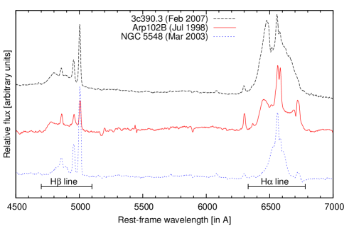
Figure 1: Examples of spectra of objects from our monitoring campaign: 3C 390.3, Arp 102B, and NGC 5548. The dates of observations are given in brackets.

3 Methodology

Before describing in details the two used method, we outline the basics of the CCF analysis, that is a standard tool in the time series analysis. The CCF is used as a measure of the similarity or correlation between two time series (i.e., light curves) as a function of the time shift between them. Its formal description is

$${CCF(\tau)=\frac{E\left[(s(t)-\bar{s})(p(t+{\tau})-\bar{p})\right]}{\sqrt{V_{s}V_{p}}}}$$ (1)

where $s(t)$ and $p(t)$ are two light curves, $\tau$ is the time lag, $\bar{s}$, $\bar{p}$ are the means of the corresponding light curves, and ${V}_{s},{V}_{p}$ are the variances of the corresponding light curves. The time lag $\tau$ corresponding to the peak in the CCF is quantifying the delay between two time series.

Eq. (1) assumes an uniform sampling in the light curves, but since this is not usually the case some approximative methods have to be employed for providing the uniform sampling. A well known approximation technique is the ICCF method given by Gaskell & Peterson (1987) (which was later modified by White & Peterson, 1994; Peterson et al., 1998, 2004) based on a linear interpolation scheme which allows to determine the missing data in the light curve. In this method the cross-correlation is performed twice: first time series is interpolated and correlated with the second one, and vice versa. The average is taken for the final result. So, the form of the ICCF, when the interpolation is performed in time series $p(t)$ is given as

$${ICCF(\tau)=\frac{1}{N}\sum\frac{(s_{i}(t)-\bar{s})\left[L_{p}\left[p(t+{\tau})\right]-\bar{p}\right]}{\sqrt{{\sigma}_{s}{\sigma}_{p}}}}$$ (2)

where $\rm L_{p}$ is a piecewise linear interpolation of the time series $p$ at $t+\tau$, $N$ is the number of data in time series $s$, and $\sigma_{s}$, $\sigma_{p}$ are standard deviations of the corresponding time series. While $\bar{s}$, $\bar{p}$ have been already defined above. The ICCF works well if assuming that the variations in the light curve are smooth.

Another method, is the DCF (Edelson & Krolik, 1988) which utilizes a binning scheme to approximate the missing data. In this procedure, pairwise combinations of measured flux values from the two light curves are binned according to their relative delays or lags. For the data pairs within each lag bin, a quantity which is essentially a Pearsons linear correlation coefficient is computed (Press et al., 1992). This technique estimates CCF with

$${DCF(\tau)=\frac{1}{M_{\tau}}\sum_{(i,j)\in K}\frac{(s_{i}-\bar{s})(p_{j}-\bar{p})}{\sqrt{\sigma_{s}\sigma_{p}}}}$$ (3)

where $s_{i}$ and $p_{j}$ are pair of i-th and j-th data points from the first and the second light curves, respectively, in the collection K of i and j within selected bin $M_{\tau}$ at $\tau-{\frac{\Delta{\tau}}{2}}\leq{t_{j}-t_{i}}\leq\tau+{\frac{\Delta{\tau}}{2}}$, and $\Delta{\tau}$ is a chosen bin size. The errors in the DCF are estimated from the standard deviation in each bin.

Both the ICCF and DCF methods are widely applied in the time series analyses. The algorithms and limitations of the methods have been discussed in detail by Robinson & Perez (1990) and by White & Peterson (1994), and here we just outline that the DCF does not give reasonable results for the limited number of data points. Moreover, both methods are unable to provide direct estimates of the uncertainties in the estimated lags, thus the assumption-dependent Monte Carlo simulations are used. Also, it is not clear how such operations as interpolation and rebinning will change the result of the analysis.

Further, we describe in details the two CCF techniques applied in this paper.

3.1 Z-transformed Discrete Correlation Function (ZDCF)

Another common method used to estimate the CCF of non uniformly sampled light curves is the ZDCF (see Alexander, 1997, 2013). This is also a binning algorithm and can be considered as a modification of the DCF technique, in which all points from the two light curves are ordered according to their time difference $\tau_{ij}$, and binned according to the user’s perception. The ZDCF scheme is based on the approximation of the cross-correlation function CCF($\tau$) with the correlation coefficient between the two time series. It is defined as:

$${r=\sum_{i=1}^{n}\frac{(s_{i}-\bar{s})(p_{i}-\bar{p})}{{(n+1)S}_{s}{S}_{p}}}$$ (4)

where $n$ is the number of time series pairs in a given time lag bin and, in difference to the DCF where the normalization is by the mean and standard deviation of the whole time series. The variances $S_{s}^{2}$ and $S_{p}^{2}$ are used to normalize each individual bin. Therefore, the ZDCF is normalized by the mean and standard deviation of the cross correlated light curves using only the data points that contribute to the calculation of each lag, i.e. called ’local CCF’ (Welsh, 1999). The method uses the Fisher’s z-transform of $r$ (Fisher, 1920) to estimate the confidence level of a measured correlation, where the binning is defined by the equal population rather than the equal width $\Delta{\tau}$. The z-transform’s convergence requires a minimum of $n_{min}=11$ points per bin (Alexander, 1997, 2013).

For equal binning, the ZDCF estimates of the CCF are equal to the DCF results, but the uncertainties are better behaved. However, it has been shown that the calculation of the ZDCF is more robust than the ICCF and DCF methods when applied to very sparsely and irregularly sampled light curves (see e. g., Edelson et al., 1996; Alexander, 1997a; Chiang et al., 2000; Giveon et al., 1999; Roy et al., 2000; Liu et al., 2008, 2011; Alexander, 2013). This method has advantage on our light curves which have more sparse data by nature. More details will be discussed in Section 4.1. The ZDCF method determines the peak of ZDCF profile and the corresponding lag uncertainty with maximum likelihood function on a large number of Monte Carlo simulations.

3.2 Stochastic Process Estimation for AGN Reverberation (SPEAR)

Beside CCF methods which measure the time delay between the continuum and emission-line variations, Zu et al. (2011) recently provided an alternative method of measuring reverberation time lags called Stochastic Process Estimation for AGN Reverberation (SPEAR).

The SPEAR method treats gaps in the temporal coverage of light curves in a well defined statistical approach. For any given damped random walk (DRW) model parameters, the stochastic process model not only interpolates between data points, but also self-consistently estimates and includes the uncertainties in the interpolation. The method can: i) separate light curve means, trends, and systematic errors from variability signals and measurement noise in a self-consistent way, ii) derive lags of multiple emission lines and their covariances simultaneously, and iii) provide statistical confidence limits on the lag estimates as well as other parameters.

The fundamental idea of the DRW model is that the variability of signal $s(t)$ (e.g. continuum) has one simple exponential covariance between two different epochs $t_{i}$ and $t_{j}$, in a form

$${<s(t_{i})s(t_{j})>={\sigma}^{2}\cdot exp^{\frac{-\left|{t_{i}}-{t_{j}}\right|}{\tau_{0}}}.}$$ (5)

Then, through the two DRW parameters, the damped intrinsic variability time-scale $\tau_{0}$ and the damped intrinsic variability amplitude $\sigma$, the AGN variabilities in both observed and unobserved epochs can be well reproduced.

The covariance between line signal $s_{l}$, and continuum signal $s_{c}$, can be defined as

$${<s_{l}(t_{i})s_{c}(t_{j})>=\int dt^{\prime}g(t_{i}-t^{\prime})<s_{c}(t^{\prime})s_{c}(t_{j})>}$$ (6)

Here we assumed that a simple top hat function $g(t-t^{\prime})=A\cdot\Delta\tau,(t-t^{\prime})\in[t_{1},t_{2}]$, which has a mean lag $<\tau>=(t_{1}+t_{2})$ and temporal width $\Delta\tau=t_{2}-t_{1}$. The scaling coefficient $A$ determines the line response for a given change in the continuum, but SPEAR largely views it as a nuisance variable.

The SPEAR method provides confidence limits for all parameters through calculation of the Highest Posterior Density (HPD) intervals. The logarithmic likelihood value of these parameters are calculated. The ratio log-likelihood functions of this method is defined in the following form

$${L=-2\cdot ln(\frac{\mathcal{L}}{\mathcal{L}_{max}})}$$ (7)

The likelihood $\mathcal{L}$ is defined in Eq. (17) in Zu et al. (2011) and is proportional to $e^{\frac{-\chi^{2}}{2}}$. The best model, corresponding to $\mathcal{L}_{max}$, is associated with the minimum $\chi^{2}$ of the lag model, thus minimizing L in Eq. 5, as it is shown in Grier et al. (2012), the following formula is obtained

$${\Delta\chi^{2}=-2\cdot ln(\frac{\mathcal{L}}{\mathcal{L}_{max}}).}$$ (8)

Based on this considerations, this measures $\Delta\chi^{2}$ between models using each lag and the best model.

The SPEAR method has been successfully used to improve reverberation mapping measurements (Grier et al., 2012; Dietrich et al., 2012), providing velocity-delay maps (Grier et al., 2013a), and the super massive black hole mass estimates (Grier et al., 2013b). The difference between the SPEAR and classical cross-correlation methods are in two basic aspects: i) SPEAR explicitly models the light curve and transfer function and fits it to the continuum and the line data, maximizing $\mathcal{L}$ of the model and then computing uncertainties using the Markov chain Monte Carlo method; ii) SPEAR models the continuum light curve as an autoregressive process using a DRW model where a self-correcting term is added to a random walk model to confine any deviations back toward the mean value. The parameters of the DRW model are included in the fits and their uncertainties, as it is a top-hat model of the transfer function and the light curve means. This auto-regressive process has been demonstrated using large samples of quasar light curves to be a valid statistical representation of quasar variability (Gaskell & Peterson, 1987; Kelly et al., 2009; Kozlowski et al., 2010; MacLeod et al., 2010; Meusinger et al., 2011; Bailer-Jones, 2012; Andrae et al., 2013; Zu et al., 2013).

4 Results

4.1 The ZDCF analysis

We apply the ZDCF method to the continuum and emission-line light curves of Arp 102B, 3C 390.3, NGC 5548, and NGC 4051, considering the continuum measurements as the first time series and the line flux as the second one. The results from the ZDCF analysis are presented in Fig. 2 and Table 2. In Fig. 2 the ZDCF correlation coefficients as a function of time lag are shown, where the horizontal and vertical error bars represent the $1\sigma$ intervals in the time lags and correlation coefficients, respectively. Table 2 summarizes the following ZDCF parameters for each object: the time lag with the maximum likelihood coefficient $\tau_{ML}$ , the peak of ZDCF curve $r_{\rm max}$, and the value of maximum likelihood parameter ML. $\bar{P_{cont}}$, $\tilde{P_{cont}}$ are the mean and median sampling periods for the continuum and $\bar{P_{line}}$, $\tilde{P_{line}}$ are the mean and median sampling periods for the line light curves, respectively, while N1 and N2 are the total number of points in the corresponding light curve. We use median vales for sampling period because median is much more resistant to outliers than is the mean. The time lag ($\tau_{ML}$) is basically the location of the peak of the correlation coefficient nearest to the zero lag, and it also has the largest maximum likelihood parameter. In the case of H${\alpha}$ line of Arp 102B, in addition to the lag of around 15 days, there is also a lag of ${157.90}_{-46.33}^{+20.3}$ days, with large maximum likelihood of 0.87. Therefore we also list this result. In Table 2 the peak of maximum likelihood can be better determined in the case with more sampling points, as H$\alpha$ of Arp 102B and 3C 390.3 make it evident.

Table 2: The ZDCF method results applied on the continuum (first time series) and emission line (second time series). The positive lags mean that the second time series is delayed relative to the first. In case of Arp 102B first two time lags are given. See text for details.

Object	Time series 1	${\bar{P_{cont}}}$	$\tilde{P_{cont}}$	N1	Time series 2	${\bar{P_{line}}}$	$\tilde{P_{line}}$	N2	$\tau_{ML}$	$r_{max}$	ML
	continuum	(days)	(days)		emission line	(days)	(days)		(days)	(days)
Arp 102B	red	96.88	28.96	88	H$\alpha$	94.66	28.96	90	${15.0}_{-13.8}^{+24.4}$	$0.20_{-0.14}^{+0.14}$	0.79
									${157.1}_{-110.1}^{+20.3}$	$0.39_{-0.22}^{+0.21}$	0.87
	blue	73.08	20.98	116	H$\beta$	40.43	17.1	110	${22.8}_{-20.9}^{+64.0}$	$0.23_{-0.1}^{+0.09}$	0.995
3C 390.3	5100 Å	128.61	108.6	34	H$\alpha$	128.67	92.9	34	${23.9}_{-10.5}^{+95.8}$	$0.90_{-0.06}^{+0.05}$	0.47
	5100 Å	35.78	22.7	129	H$\beta$	35.78	22.7	129	$94.5_{-48.0}^{+27.1}$	$0.94_{-0.03}^{+0.02}$	0.60
NGC 5548	5190 Å	28.35	7.29	81	H$\alpha$	42.42	9.48	56	$27.0_{-5.7}^{+14.4}$	$0.87_{-0.05}^{+0.04}$	0.99
	5190 Å	28.35	7.29	81	H$\beta$	28.11	7.53	84	$49.2_{-7.7}^{+18.6}$	$0.90_{-0.03}^{+0.03}$	0.997
NGC 4051	5100 Å	0.57	0.45	233	H$\beta$	1.08	1.0	108	$2.6_{-1.1}^{+0.9}$	$0.49_{-0.08}^{+0.08}$	0.43

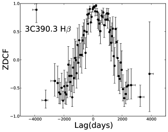
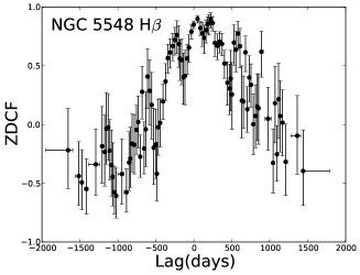
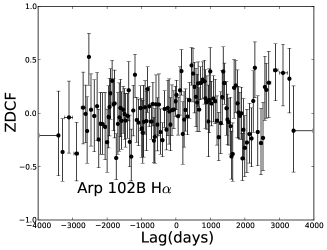
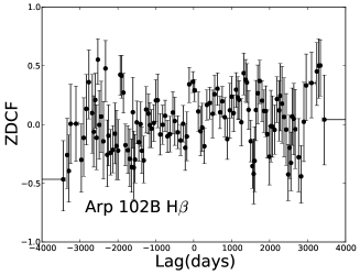
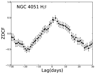
Figure 2: The ZDCF analysis of object and emission line doneted on each plot. The horizontal and vertical error bars correspond to $1\sigma$ uncertainties for a normal distribution.

Table 3: The SPEAR method results based on fitting of the continuum and emission line. The last three columns are giving the same results if the continuum and two lines (H$\alpha$ and H$\beta$) are fitted simultaneously. See text for details.

Object	Line	$\tau_{SPEAR}$	$\sigma$	$\tau_{d}$	$\tau_{SPEAR}^{\star}$	$\sigma^{\star}$	$\tau_{d}^{\star}$
Arp 102B	H$\alpha$	${23.8}_{-18.8}^{+27.5}$	0.069	45.15	${31.5}_{-22.1}^{+47.3}$	0.662	430
	H$\beta$	${47.6}_{-37.2}^{+57.2}$	0.095	45.51	${42.2}_{-27.5}^{+49.7}$
3C 390.3	H$\alpha$	${43.8}_{-34.8}^{+48.6}$	0.82	1382.0	${77.4}_{-59.0}^{+90.4}$	0.92	1025
	H$\alpha$	${150.9}_{-143.8}^{+157.5}$	0.82	1732.0
	H$\beta$	$76.9_{-74.7}^{+79.1}$	0.94	1147	$76.0_{-55.0}^{+78.8}$
NGC 5548	H$\alpha$	$43.5_{-39.3}^{+47.7}$	0.25	476.38	$45.5_{-39.9}^{+49.1}$	0.273	475
	H$\beta$	$45.4_{-43.0}^{+47.0}$	0.27	415.45	$43.4_{-38.4}^{+47.4}$
NGC 4051	H$\beta$	$2.8_{-2.3}^{+3.1}$	0.005	5.58

4.2 The SPEAR analysis

In order to perform SPEAR analysis , we build the continuum model to determine the DRW parameters of the continuum light curves for all four objects. Then, in order to measure the time lag between the continuum and H${\alpha}$ and H${\beta}$, SPEAR interpolates the continuum based on the posteriors derived, and then shifts, smooths, and scales each continuum light curve to compare to H${\alpha}$ and H${\beta}$.

Examples of the mean light curve models of the continuum and emission line, obtained by the SPEAR fitting, are presented in Fig. 3. Fig. 4 gives $\Delta\chi^{2}$ from Eq. (5) between models. The time lag values $\tau_{SPEAR}$, the updated posteriors of the damping time scale $\tau_{d}$ and the variability amplitude $\sigma$ are given in Table 3. The values obtained from fitting the continuum and a single line are given in the first set of columns. The results for fitting the continuum and both H$\alpha$ and H$\beta$ line simultaneously with SPEAR method are also given in Table 3 (last three columns). The values of $\tau_{\rm SPEAR}$ for H$\alpha$ and H$\beta$ obtained from simultaneous fitting procedure are slightly different. The contrast arises from differences in sampling periods and number of data points of continuum curves around H$\alpha$ and H$\beta$ lines respectively (see Table 2). E. g, SPEAR simultaneous procedure has been applied on two types of set of curves. The first model consisted of the continuum around H$\alpha$ line, the H$\alpha$ line (as the first line) and H$\beta$ line (as the second), while the second model consisted of the continuum around H$\beta$ line, H$\beta$ line (as the first line) and H$\alpha$ (as the second line).

The slow (or lack of) convergence and existence of multiple peaks of the log-likelihood function (Fig. 4) could be influenced by: sampling characteristics of data set (Zu et al., 2011), the relationship among variables of set of observations as well as their values even in the case of well sampled data (Grier et al., 2012). In the case of our data set of NGC 5548, H$\alpha$ line’s average sampling period is twice larger than both the continuum and H$\beta$ line, while median sampling periods are almost similar. The average sampling periods of Arp 102B H$\alpha$ line and corresponding continuum are quite large (about 100 days, almost 3 times larger than median sampling period, which indicates skewness of its data distribution).

In the case of H$\alpha$ and continuum of 3C 390.3, the both the median and average sampling periods are the largest among the sample of AGNs. Its log-likelihood function shows two peaks and slow convergence. The curves are actually modeled as a Gaussian process, while in principle there could be deviations of light curves from Gaussian process infecting the fitting parameters. The large multi-year gaps in the data would result in weaker constraints on the final model fit, since the covariance matrix is calculated for given differences between observational times. Also, the parameters $\tau_{d}$ and $\sigma_{d}$ are found to be correlated with the physical properties of accretion disks, including optical luminosities, Eddington ratios, and black hole masses, which also could affecting fitting results of the SPEAR method (DRW is actually phenomenological model).

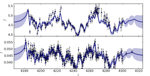
(a) NGC 4051, top: cont., bottom: H${\beta}$ line

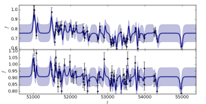
(b) Arp 102B, top: cont., bottom: H${\alpha}$ line

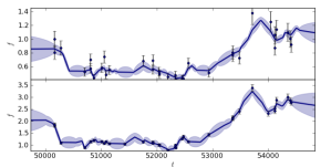
(c) 3C 390.3, top: cont., bottom: H${\alpha}$ line

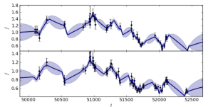
(d) NGC 5548, top: cont., bottom: H${\beta}$ line

Figure 3: The predicted mean light curves from the best-fit SPEAR model of the continuum (upper plots) and one emission line (bottom plots). The units in the case of NGC 4051 are $10^{-15}{\rm erg\,s^{-1}cm^{-2}}$ Å ^-1 for continuum, and $10^{-11}{\rm erg\,s^{-1}cm^{-2}}$ Å ^-1 for H${\beta}$, while in case of other objects the normalized light curves are given. The black points with error bars show the observed light curves, the solid line shows the mean of the SPEAR light curve models fit to the observed data, and the blue bands present the standard deviation (see Zu et al., 2011).

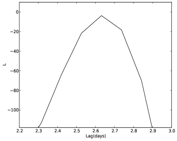
(a) NGC 4051,H$\beta$ line

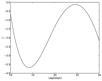
(b) Arp 102B,H$\alpha$ line

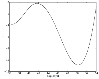
(c) NGC 5548,H$\alpha$ line

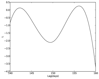
(d) 3C 390.3,H$\alpha$ line

Figure 4: The ratio of log-likelihood functions from the SPEAR analyses. The y-axis shows the SPEAR likelihood ratios for continuum and single emission line as labeled. The log-likelihood ratio is negative since it is calculated for a simple vs simple hypothesis. The number of parameters in the models are the same, while the range of lag is varied: wider range and narrower range around obtained lag. The ranges of time lag $\tau$ used in fitting procedure are enclosing time lags obtained from continuum+one line and unique solution obtained from continuum+two line fitting procedure. The unique solution obtained from continuum+two line fitting eliminates spurious lags. The ratio of log likelihoods can not pass the narrower range of lags used in testing hypothesis. In the case of 3C 390.3 is given ratio log-likelihoods for range of time lag enclosing the secondary solution from continuum+one line fitting SPEAR’s procedure.

5 Discussion

For comparison, we summarize the time lag measurements given in the literature for these 4 objects in Table 4. Our results from both methods are comparable (not congruent) with the earlier estimates, but some differences could be found.

The largest time lags are for 3C 390.3 and NGC 5548 (see Table 4). For 3C 390.3 the longest monitoring campaign was undertaken by Shapovalova et al. (2010) and Dietrich et al. (2012). Analyzing the discrepancy between the time lags obtained from these two campaigns, Dietrich et al. (2012) found that the properties of the continuum strength variations have a significant effect on the time delay obtained using CCF. Also, Sergeev et al. (2002, 2011) noted that the width of the auto-correlation function (ACF) of the continuum light curve which is covering several years up to more than a decade is much broader than the ACF of a shorter campaign, and that this will result in a longer time delay. Since the CCF is the convolution of the transfer function with ACF of the continuum, and the ACF is a symmetric function, asymmetric properties of the transfer function (e.g. the position of the peak) must be reflected in a similar manner in the CCF (e. g. Mrk 50; Pancoast et al., 2012). However, it is also possible that changes in the measured cross-correlation lag arise from changes in the continuum ACF rather than in the delay-map (see Robinson & Perez (1990), Perez et al. (1992a), Perez et al. (1992b), Welsh (1999)). If the continuum variations become slower, a sharp peak at low time-delay in the delay distribution will be blurred by the broader ACF, and the peak of the CCF will be shifted to larger delays (Netzer & Maoz, 1990). Thus, the lag measured by cross-correlation analysis depends not only on the delay distribution, transfer function, but also on the characteristics ACF of the continuum variations. The monitoring campaining of Dietrich et al. (2012) lasted for 80 days and they could not measure longer delays. On the other hand, wider temporal sampling of the long monitoring campainings could affect results too. For NGC 5548, our calculations produced larger values for H$\beta$ time lags, while for NGC 4051 we could see that time lag obtained by Denney et al. (2009b) is about 3 times smaller than the value obtained by Peterson et al. (2000), and our calculation confirms value of about 2.5 days.

Table 4: Time lag measurements for Arp 102B, 3C 390.3, NGC 5548, and NGC 4051.

Object	Continuum waveband	Line	$\tau$	Method used	References
	(in Å )		(days)
Arp 102B	cnt 6368-6412	H$\alpha$	$13_{-105}^{14}$	ICCF	Sergeev et al. (2000)
	cnt 6356-6406	H$\alpha$	$15_{-13.8}^{15.7}-17_{-14.3}^{14.3}$	ZDCF	Shapovalova et al. (2013)
			$23_{-30.2}^{16.8}$	SPEAR	Shapovalova et al. (2013)
	cnt 6356-6406	H$\alpha$	$15_{-13.8}^{24}$,$24_{-18.8}^{27.5}$	ZDCF,SPEAR	this work
	cnt 5200-5250	H$\beta$	$11_{-9.8}^{19.3}-21_{-19}^{54.3}$	ZDCF	Shapovalova et al. (2013)
			$37_{-47.5}^{19.7}$	SPEAR	Shapovalova et al. (2013)
	cnt 5200-5250	H$\beta$	$23_{-20.9}^{64}$,$48_{-37}^{57}$	ZDCF,SPEAR	this work
3C 390.3	cnt 4400-9000	H$\alpha$	$20\pm 8$	ICCF+ZDCF+DCF	Dietrich et al. (1998)
	cnt 6484-6608	H$\alpha$	$162_{-15}^{32}$	ICCF	Sergeev et al. (2002)
	cnt 5369-5399	H$\alpha$	$23_{-7}^{5}$	ZDCF+ICCF	Shapovalova et al. (2010)
	cnt 6200	H$\alpha$	$174\pm 16$	ICCF	Sergeev et al. (2011)
	cnt 5100	H$\alpha$	$56.3_{-6.6}^{2.4}$	ICCF	Dietrich et al. (2012)
			$52.5_{-0.6}^{0.7}$	SPEAR	Dietrich et al. (2012)
	cnt 5369-5399	H$\alpha$	$24_{-10.5}^{95.8}$,$44_{-35}^{49}$	ZDCF,SPEAR	this work
	cnt 4400-9000	H$\beta$	$20\pm 8$	ICCF+ZDCF+DCF	Dietrich et al. (1998)
	cnt 4400-9000	H$\beta$	$24.2_{-8.4}^{6.7}$	photoiozination	Wandel et al. (1999)
	cnt 5000-5006	H$\beta$	$50_{-10}^{100}$	ICCF	Peterson et al. (2004)
	cnt 5370-5420	H$\beta$	$100_{-97}^{101}$	ICCF	Shapovalova et al. (2001)
	cnt 5360-5425	H$\beta$	$89_{-10}^{12}$	ICCF	Sergeev et al. (2002)
	cnt 5369-5399	H$\beta$	$96_{-47}^{28}$	ZDCF+ICCF	Shapovalova et al. (2010)
	cnt 5100	H$\beta$	$94\pm 16$	ICCF	Sergeev et al. (2011)
	cnt 5100	H$\beta$	$44.3_{-3.3}^{3}$	ICCF	Dietrich et al. (2012)
			$47.9_{-4.2}^{2.4}$	SPEAR	Dietrich et al. (2012)
	cnt 5369-5399	H$\beta$	$95_{-48}^{27}$,$77_{-75}^{79}$	ZDCF,SPEAR	this work
	cnt 4400-9000	H$\gamma$	$20\pm 8$	ICCF+ZDCF+DCF	Dietrich et al. (1998)
	cnt 5100	H$\gamma$	$58.1_{-6.1}^{4.3}$	ICCF	Dietrich et al. (2012)
			$32.1\pm 17.3$	SPEAR	Dietrich et al. (2012)
	cnt 5100	HeII	$22.3_{-3.8}^{6.5}$	ICCF	Dietrich et al. (2012)
			$36\pm 5.2$	SPEAR	Dietrich et al. (2012)
	cnt 1330-1470	Ly$\alpha$	$69_{-19}^{50}-108_{-21}^{15}$	ICCF+DCF	Wamsteker et al. (1997)
	CIV		$49_{-17}^{13}-63_{-20}^{57}$		Wamsteker et al. (1997)
	cnt 1340-1400	Ly$\alpha$	$34\pm 17$	ICCF+DCF	O Brien et al. (1998)
	CIV		$66\pm 35$		O Brien et al. (1998)
NGC 5548	cnt 6300-6350	H$\alpha$	$11.02_{-1.15}^{1.27}$	ICCF	Bentz et al. (2010a)
	cnt 5190	H$\alpha$	$27_{-6}^{14}$,$43_{-39}^{48}$	ZDCF,SPEAR	this work
	cnt 5185-5195	H$\beta$	$6_{-4.08}^{4.44}-26.4_{-2.63}^{4.67}$	ICCF	Peterson et al. (2002)
	cnt 5170-5200	H$\beta$	$6.5_{-2.5}^{2.5}$	ICCF+DCF	Bentz et al. (2007)
	cnt 4800-4830	H$\beta$	$18_{-5}^{5.8}-25_{-1.5}^{1.4}$	ICCF	Sergeev et al. (2007)
	cnt 5150-5200	H$\beta$	$4.25_{-1.33}^{0.88}$	ICCF	Bentz et al. (2009)
	cnt 6300-6350	H$\beta$	$4.25_{-1.33}^{0.88}$	ICCF	Bentz et al. (2010a)
	cnt 5190	H$\beta$	$49_{-7.7}^{19},45_{-43}^{47}$	ZDCF,SPEAR	this work
	cnt 6300-6350	H$\gamma$	$1.25_{-2.34}^{1.86}$	ICCF	Bentz et al. (2010a)
NGC 4051	cnt 5100-6800	H$\alpha$	$3.1\pm 1.6$	DCF	Shemmer et al. (2003)
	cnt 5090-5120	H$\beta$	$6\pm 3$	ICCF+DCF	Peterson et al. (2000)
	cnt 5100-6800	H$\beta$	$2\pm 2.3$	DCF	Shemmer et al. (2003)
	cnt 5090-5130	H$\beta$	$1.87_{-0.5}^{0.54}$	ICCF+DCF	Denney et al. (2009c)
	cnt 5100	H$\beta$	$3.5_{-0.5}^{12}$	ICCF	Yang et al. (2013)
	cnt 5190	H$\beta$	$3_{-1.1}^{0.9},3_{-2.3}^{3.1}$	ZDCF,SPEAR	this work

In order to test the statistical relationship between the ZDCF and SPEAR results, we calculated the Pearson correlation coefficient $r$ and the p-value between different sets of time lags, which confirmed that results obtained from H$\alpha$ of 3C 390.3 are an outlier. Such behavour of H$\alpha$ line of this object could have roots in bad median and average sampling period and very broad the ACF of the continuum and the line itself.

The secondary (spurious) time lags are obtained for H$\alpha$ lines of Arp 102B and 3C 390.3. These spurious lags could arise due to the fact that the H$\alpha$ line and continuum of both objects have large sampling period. In the case of 3C 390.3 average and median sampling periods are larger than 100 days and in the case of Arp 102B average sampling period is 100 days. The median value is three times smaller, indicating skewness of data distribution. Other two objects have much smaller sampling periods. The ACF of continuum and H$\alpha$ of 3C 390.3 are very broad, which can also lead to spurious large values of CCF (see Welsh, 1999). As for the secondary lag of Arp 102B, we noticed that the autocorrelation functions of continuum and H$\alpha$ line are noisy and similar to each other (it could be a consequence of irregular sampling and physical nature of light curves itself).

Since we have spurious time lags, we defined both sets with and without these values. We found the strongest correlation ($r\sim 0.9$) between the ZDCF and one-line SPEAR fitting time lags (when spurious lags of H$\alpha$ of Arp 102B and 3C 390.3 are excluded in ZDCF and SPEAR sets, respectively). Also, we found a weaker correlation between the sets of ZDCF time lags (without spurious lag included, the unique solution from SPEAR’s continuum + two line fitting procedure eliminates second peak) and two-line SPEAR fitting time lags. This is not surprising since when we fit both lines simultaneously, the light curve together with its determined lag adds extra information to the continuum light curve, and thus better constrains the another light curve’s lag. Both correlations are suggesting that these sets of time lags are reliable and linearly dependent. All other combinations which include spurious time lags of H$\alpha$ Arp 102B and 3C 390.3 in ZDCF and SPEAR sets are linearly uncorrelated, which allowed us to discard these spurious peaks.

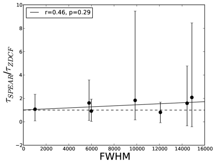
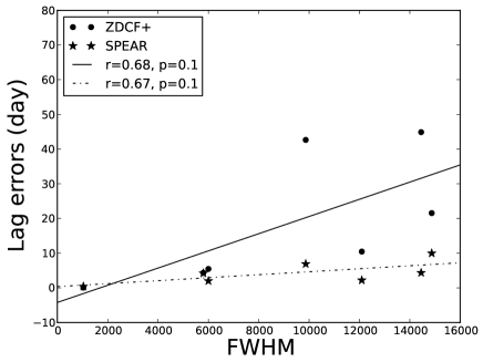
Figure 5: The ratio of the SPEAR and ZDCF time lags as a function of the FWHM of analyzed lines (upper plot), and the SPEAR and ZDCF lag errors as a function of the FWHM (bottom plot). The horizontal dashed line on upper plot enhances visibility of depicted trend. The Pearson correlation coefficient $r$ and the p-value are indicated in the upper left corner.

We also probe the correlation between the sets of calculated time lags, their errors and emission line widths (see Fig. 5). For the line widths we use the Full Width Half Maximum (FWHM) of the RMS profiles of H${\alpha}$ and H${\beta}$, taken from Shapovalova et al. (2013) for Arp 102B, Shapovalova et al. (2010) for 3C 390.3, Shapovalova et al. (2004) for NGC 5548, and Denney et al. (2009c) for NGC 4051. In the upper panel of Fig. 5, depicted trend of higher lag ratio with larger FWHM is not significant (see dashed line with slope 0 at lag ratio 1, passing all the error bars, without increase $\chi^{2}$ in fitting).

Obtained results are just suggesting that deviation between two methods is affected by FWHM (see Fig. 5, bellow panel), but the trend is not statistically significant. It could be seen that the ZDCF lag errors are larger than SPEAR’s. Namely, the ZDCF lag errors are calculated from fiducial distribution and the fiducial interval cannot be narrower than the bin width corresponding to maximum ZDCF value. Also, the ZDCF method bins by equal population and as a result the bins are not equal in time-lag width.

Also, the lag errors are more sensitive to the FWHM in ZDCF method than in the SPEAR one (see Fig. 5, bottom panel). A possible explanation is that the line widths influence strongly the error of time lag measurements. Consequently, this increases the uncertainty of the black hole mass. On the other hand, we found a weak correlation between the FWHM and one line SPEAR fitting time lags (without spurious time lag). The time lag in cross correlation analysis is the first moment of transfer function, and it is more sensitive to the autocorrelation function of the continuum, and because of this we can not find correlations between the ZDCF time lags and FWHM. Empirically, it is expected that the scaling coefficient A in the transfer function is inversely correlated with the ionizing continuum flux, where A is defined as $A=\frac{\left|scale_{1}\cdot scale_{2}\right|}{swid_{1}}$ (Zu et al., 2011). Parameters $scale_{1}$, $scale_{2}$, $swid_{1}$ are scale factors and tophat width obtained from posterior distribution, note that appearance of $swid_{1}$ in denominator depends on SPEAR’s input parameters.

This may cause problems in case of the light curves with the significant long term trends observed and it could be a reason for correlation between the SPEAR time lags (from one line fitting) and FWHM. Also, this should be tested on large number of simulated light curves, which will provide more insights.

The time lags from reverberation mapping provide more robust measurement on the size of the BLR comparing with estimating it from the 5100 Å  luminosity used in empirical virial masses estimate for black holes with H$\beta$ line width (Kaspi et al., 2000) and H$\alpha$ line width (Greene & Ho, 2005). Moreover, our results for the time lags of $\sim$30 ld for Arp 102B and $\sim$80 ld for 3C 390.3 are in good agreement with the estimated disk dimensions for these objects (1000 $R_{\rm G}$ and 1400 $R_{\rm G}$ given by Chen & Halpern (1989) and Flohic & Eracleous (2008), respectively) if we assume the SMBH masses of $1.1\times 10^{8}M_{\odot}$ for Arp 102B (Shapovalova et al., 2013) and $5\times 10^{8}M_{\odot}$ for 3C 390.3 (Nelson et al., 2004; Dietrich et al., 2012).

As can be shown by many studies, the choice of the method to calculate time delay should not have to be made apriori, however the unceirtainities depends directly on this decision. In our study we found that the time lags determined by the ZDCF (excluding the large value of H$\alpha$ of Arp 102B) and SPEAR (excluding large value of H$\alpha$ of 3C 390.3) methods are consistent with each other as expected. Moreover, the results are consistent with previous estimates summarized in Table 4. For example, the consistency of the SPEAR and ICCF time lags of 3C 390.3 has been confirmed (Zhang, 2013). These consistencies indicate that our procedures to estimate the time lag by the SPEAR method and by the CCF method are reliable. Hereby we note that using different collection of AGNs could bring some other conclusions. For example, in the case of H$\alpha$ 3C 390.3, that has the worst sampling rate, both methods produced largest uncertainties. However, both methods recovered successfully time lags that are consistent with previous results.

As for the advantages and disadvantages of the used methods, we can say that the broad line profiles of Arp 102B, 3C 390.3, and NGC 5548 have produced ’flat-top’ ZDCF curves, while the unfavorable sampling rate continuum and emission lines induced (Arp 102B, 3C 390.3, and NGC 5548) slow convergence of log-likelihood functions in the SPEAR method. Also, the broad line profiles could as well contribute to the slow convergence, as was noticed in case of Mrk 1501 (Grier et al., 2012), which data were well sampled however the log-likelihood function does not converge. The lines we used for the SPEAR two-line fits are pairs of two Balmer lines, which have similar low ionization levels, and this could affect the fitting results (Zu et al., 2011). Finally, the nature of the non classical BLR of Arp 102B and 3C 390.3 could affect SPEAR and ZDCF to produce larger values for H$\beta$ than for H$\alpha$ time lags. The ZDCF limitation is arising from discrete binning, which implicitly assumes that the spacing between the data points is uncorrelated with their observing times. However, if this special sampling pattern appears in given light curve, it will be reflected in spurious fluctuations between consecutive ZDCF points.

Such fluctuations disappeared only when the ZDCF bin size was enlarged, or when the data were omitted from the light curves. As for limitations of SPEAR method, it assumes that the continuum variation is a damped random walk and that the line flux should vary in a corresponding way, which could be deformed by some other known and unknown mechanisms.

Finally, the characteristics of light curves such as: irregular sampling, correlated errors, and seasonal gaps are well-known factors of quality of time-series analysis not only in the reverberation mapping campaigns, but also in all the ground-based time-domain observational studies (including black hole mass measurements) (see, e.g. Grier et al., 2008; Peterson, 2011; Zu et al., 2011). For the black hole mass estimates, among the most crucial factors is accuracy of time lag calculations. The expected accuracy of a time delay measurement depends on the number of observation (N) as follows $\sigma({\tau})\sim\frac{1}{\sqrt{N}}$ (Horne, 2013, personal communication). Sampling is contributing to the time lag measurements, in the manner as MacLeod et al. (2010) concluded that probing the timescales as short as $\frac{\tau}{10}$, ($\tau$ is damping timescale, also called the characteristic timescale) and assuming a characteristic redshift of 2 of AGN, the light curves should be sampled every 3 days in the observer’s frame. The common belief is that the time series used to compute the CCF should be at least 4 times longer than the lags of interest, and preferably $\sim 10$ times longer, which is well illustrated in Welsh (1999). Note that all our time series cover periods which are much more than 10 times longer of calculated time lags. Beside this, the length of time series is also important. As for an example, more serious problem (see Koen, 1994) than the complexity of the relation between light curves could be possible non-stationarity of such relation. Non-stationarity could be due to changes in the lag between the two series. This could be analyzed by using very long sets of observations and studying segments of the series and comparing the estimate lags. Finally, beside frequency domain methods, it is important to use more of cross-spectrum to study relation between time series (see e.g. Sriram et al., 2009).

6 Conclusion

Here we present time series analysis of the continuum and the H${\alpha}$ and H${\beta}$ lines of two well known type 1 AGNs with optical spectra showing double peaked line profiles (Arp 102B and 3C 390.3) and two well known broad line AGNs (NGC 5548 and NGC 4051 ). We used the ZDCF and the SPEAR method for time lag calculations and can outline the following conclusions:

(i) AGNs with broader emission have larger time lag uncertainties in both ZDCF and SPEAR methods. This should be taken into account for the black hole mass estimates using the virial theoreme. This should be further tested on a larger set of AGNs.

(ii) The ZDCF time lags (without large value of H$\alpha$ of Arp 102B) and SPEAR time lags (without large value of H$\alpha$ of 3C 390.3) are similar.

(iii) Based on (ii) SPEAR and ZDCF produced larger values for H$\beta$ than for H$\alpha$ time lags, especially in the case of 3C 390.3, while in the case of NGC 5548 they are closer.

Also, in the case of Arp 102B H$\alpha$ line has the time lag which is similar to the time lag of H$\beta$.

Finally, we conclude that both SPEAR and ZDCF method give similar results for time lags, that are consistent with previous measurements using ICCF methods in the literature. They are reliable for the time lag analysis of AGN continuum and emission line light curves, especially in the case of unevenly sampled data. The main advantage of SPEAR is possibility of rapid increase in the dimensionality of the problem: determination lags by fitting continuum and one line, two lines or even more lines (where empirical power spectral distribution of light curves shares the same form with the model) , while ZDCF corrects skewness of the sampling distribution of cross correlation coefficients by using z-transform. On the other hand, in the case of SPEAR, if the light curves are intrinsically noisy or the uncertainties are overly underestimated both could affect fitting results, while ZDCF method has tendency to overestimate errors.

7 Acknowledgments

This work was supported by the Ministry of Education and Science of Republic of Serbia through the project Astrophysical Spectroscopy of Extragalactic Objects (176001) and RFBR (grants N12-02-01237a, 12-02-00857a) (Russia) and CONACYT research grants 39560, 54480, and 151494 (Mexico). We are grateful for the very helpful comments from prof. Keith Horne. We would like to thank to referees for very useful and detailed remarks which allowed us to improve our manuscript.

References

- Alexander (1997) Alexander, T., Is AGN Variability Correlated with Other AGN Properties? ZDCF Analysis of Small Samples of Sparse Light Curves, Astronomical Time Series, Eds. D. Maoz, A. Sternberg, and E.M. Leibowitz, 1997 (Dordrecht: Kluwer), p. 163-166, 1997.
- Alexander (1997a) Alexander, T., Bloated stars as AGN broad-line clouds: the emission-line response to continuum variations, MNRAS, 285, 891-897, 1997a.
- Alexander (2013) Alexander, T., Improved AGN light curve analysis with the z-transformed discrete correlation function, 2013arXiv1302.1508A, 1-20, 2013.
- Andrae et al. (2013) Andrae, R. and Kim, D. W. and Bailer-Jones, C. A. L., Assessment of stochastic and deterministic models of 6304 quasar lightcurves from SDSS Stripe 82, A&A, 554, A137, 1-11, 2013.
- Bailer-Jones (2012) Bailer-Jones, C. A. L., A Bayesian method for the analysis of deterministic and stochastic time series, 546, A89, 1-16, 2012.
- Bentz et al. (2006) Bentz, M. C., Denney, K. D., Cackett, E. M., Dietrich, M. et al., A Reverberation-based Mass for the Central Black Hole in NGC 4151 ApJ, 651, Issue 2, 775-781, 2006.
- Bentz et al. (2007) Bentz, M. C., Denney, K. D., Cackett, E. M., Dietrich, M. et al, NGC 5548 in a Low-Luminosity State: Implications for the Broad-Line Region, ApJ, 662, Issue 1, 205-212, 2007.
- Bentz et al. (2008) Bentz, M. C., Walsh, J. L., Barth, A. J., Baliber, N., Bennert, N., Canalizo, G. et al ., First Results from the Lick AGN Monitoring Project: The Mass of the Black Hole in Arp 151, ApJL, 689, L21-L24, 2008.
- Bentz et al. (2009) Bentz, M. C., Walsh, J. L., Barth, A. J., et al., The Lick AGN Monitoring Project: Broad-line Region radii and black hole masses from reverberation mapping of H, ApJ, 705, 199-217, 2009.
- Bentz et al. (2010) Bentz, M. C., Horne, K., B. J., Bennert, V. N., et al., The Lick AGN Monitoring Project: velocity-delay maps from the maximum-entropy method for Arp 151, ApJ Letters, 720, 1, L46-L51, 2010.
- Bentz et al. (2010a) Bentz, M. C., Walsh, J. L., Barth, A. J., Yoshii, Y. et al., The Lick AGN monitoring project: Reverberation mapping of optical hydrogen and helium recombination Lines, ApJ, 716, 993-1011, 2010a.
- Cackett & Horne (2006) Cackett, E. M., & Horne, K.,Photoionised Hbeta emission in NGC 5548: It Breathes!, MNRAS, 365,1180-1190, 2006.
- Chen & Halpern (1989) Chen, K., & Halpern, J. P., Structure of line-emitting accretion disks in active galactic nuclei - Arp 102B, ApJ, 344, 115-124, 1989.
- Chen et al. (1989) Chen, K., Halpern, J. P., & Filippenko, A. V., Kinematic evidence for a relativistic Keplerian disk - Arp 102B, ApJ, 339, 742-751,1989.
- Chiang et al. (2000) Chiang, J., Reynolds, C. S., Blaes, O. M., Nowak, M. A., Murray, N. et al., Simultaneous EUVE/ASCA/RXTE observations of NGC 5548, ApJ, 528, 292-305, 2000.
- Denney et al. (2006) Denney, K. D., Bentz, M. C., Peterson, B. M., Pogge, R. W., et al.,The Mass of the Black Hole in the Seyfert 1 Galaxy NGC 4593 from Reverberation Mapping ,ApJ, 653, Issue 1, 152-158, 2006.
- Denney et al. (2009a) Denney, K. D., Peterson, B .M, Dietrich, M., Vestergaard, M., & Bentz, M. C., Systematic uncertainties in black hole masses determined from single epoch spectra, ApJ, 692, 246–264, 2009a.
- Denney et al. (2009b) Denney, K. D., Peterson, B. M., Pogge, R. W., et al., Diverse kinematic signatures from reverberation mapping of the Broad-Line Region in AGNs, ApJ, 704, L80-L84, 2009b.
- Denney et al. (2009c) Denney, K. D., Watson, L. C., Peterson, B. M., Pogge, R. W., et al., A Revised Broad-line Region Radius and Black Hole Mass for the Narrow-line Seyfert 1 NGC 4051, ApJ, 702, Issue 2, 1353-1366, 2009c.
- Denney et al. (2011) Denney, K. D., Assef, R. J., Bentz , M. C, Dietrich, M., Horne, K., Kochanek, C. S, Mathur, S., Peterson, B. M., Pogge, R. W., & Vestergaarda, M., Addressing systematic uncertainties in black hole mass measurements, in Narrow-Line Seyfert 1 Galaxies and their place in the Universe, Proceedings of Science, POS(NLS1)032, 1-14, 2011.
- Dietrich et al. (1998) Dietrich, M., Peterson, B. M., Albrecht, P., Altmann, M., Barth, A. J., Bennie, P. J., & Bertram, R., Steps toward Determination of the Size and Structure of the Broad-Line Region in Active Galactic Nuclei. XII. Ground-based Monitoring of 3C 390.3, ApJS, 115, 185–, 1998.
- Dietrich et al. (2012) Dietrich, M., Peterson,B. M., Grier, C., & Bentz, M. C., Optical monitoring of the broad-line radio galaxy 3C 390.3, ApJ, 757, 53 , 1-22, 2012.
- Edelson & Krolik (1988) Edelson, R. A., & Krolik, J. H., The discrete correlation function - A new method for analyzing unevenly sampled variability data, ApJ, 333, 646-659, 1988.
- Edelson et al. (1996) Edelson, R. A., Alexander, T., Crenshaw, D. M., Kaspi, S., Malkan, M. A., Peterson, B. M. et al., Multiwavelength observations of short-timescale variability in NGC 4151. IV. Analysis of Multiwavelength Continuum Variability ,ApJ,470, 364-377, 1996.
- Eracleous et al. (1997) Eracleous, M., Halpern, J., Gilbert, A., Newman, J. A., & Filippenko, A. V., Rejection of the Binary Broad-Line Region interpretation of double-peaked emission lines in three Active Galactic Nuclei, ApJ, 490, 216-226, 1997.
- Eracleous et al. (2009) Eracleous, M., Lewis, K. T., & Flohic, H. M. L. G., Double-peaked emission lines as a probe of the broad-line regions of active galactic nuclei, NewAR, 53, 133-139, 2009.
- Fisher (1920) Fisher, R. A., Accuracy of observation, A mathematical examination of the methods of determining, by the mean error and by the mean square error , MNRAS, 80, 758-770, 1920.
- Flohic & Eracleous (2008) Flohic, H. M. L. G., & Eracleous, M., Interpreting the Variability of Double-Peaked Emission Lines in Active Galactic Nuclei with Stochastically Perturbed Accretion Disk Models, Ap J, 686, 1, 138-147, 2008.
- Gaskell & Sparke (1986) Gaskell, C. M., & Sparke, L. S., Line variations in quasars and Seyfert galaxies,ApJ, 305, 175-186, 1986.
- Gaskell & Peterson (1987) Gaskell, C. M.,& Peterson, B. M., The accuracy of cross-correlation estimates of quasar emission-line region sizes ApJSS, 65, p. 1-11, 1987.
- Gezari et al. (2007) Gezari, S., Halpern, J. P., & Eracleous, M., Long-Term profile variability of double-peaked emission lines in Active Galactic Nuclei, ApJS, 169, 167-212, 2007.
- Giveon et al. (1999) Giveon, U., Maoz, D., Kaspi, S., Netzer, H., & Smith, P. S., Long-term optical variability properties of the Palomar-Green quasars, MNRAS,306,637-654, 1999.
- Greene & Ho (2005) Greene, J. & Ho, L. C., Estimating Black Hole Masses in Active Galaxies using the H emission line, ApJ, 630, 122, 2005.
- Grier et al. (2008) Grier, C. J., Grier, C. J., Peterson, B. M., Bentz, M. C., Denney, K. D. et al., The mass of the black hole in the quasar PG 2130+099, ApJ, 688, 837-843, 2008.
- Grier et al. (2012) Grier, C. J., Peterson, B. M., Pogge, R. W., Denney, K. D., Bentz, M. C. et al., Reverberation Mapping Results for Five Seyfert 1 Galaxies,755, 60, 1–16, 2012.
- Grier et al. (2013a) Grier, C. J., Peterson, B. M., Horne, K., Bentz, M. C., Pogge, R. W., Denney, K. D., et al., The Structure of the Broad-line Region in Active Galactic Nuclei. I. Reconstructed velocity-delay maps, ApJ, 764, 1, 1-47, 2013a.
- Grier et al. (2013b) Grier, C. J. and Martini, P. and Watson, L. C. and Peterson, B. M., Bentz, M. C. et al., Stellar velocity dispersion measurements in high-luminosity quasar hosts and implications for the AGN black hole mass scale, ApJ, 773, id90, 2013b.
- Halpern (1990) Halpern, J. P., Line emission from another relativistic accretion disk - 3C 332, ApJ, 365, L51-L54, 1990.
- Horne et al. (1991) Horne, K., Welsh, W. F., & Peterson, B. M., Echo mapping of broad H-beta emission in NGC 5548, ApJ,Part 2 - Letters, 367, L5-L8, 1991.
- Horne (1999) Horne, K., Echo mapping of agn emission regions, in quasars and cosmology, ASP Conference Series 162, Edited by G. Ferland and J. Baldwin, Astronomical Society of the Pacific (San Francisco), 189-212, 1999.
- Horne et al. (2004) Horne, K., Peterson, B. M., Collier, S. J., & Netzer, H., Observational requirements for high-fidelity reverberation mapping, PASP, 116, 465-476, 2004.
- Kaspi et al. (2000) Kaspi, S., Smith, P. S., Netzer, H., Maoz, D., Jannuzi, B. T. & Giveon, U., Reverberation Measurements for 17 Quasars and the Size-Mass-Luminosity Relations in Active Galactic Nuclei, ApJ, 533, 631-649, 2000.
- Kelly et al. (2009) Kelly, B. C., Bechtold, J., & Siemiginowska, A., Are the variations in quasar optical flux driven by thermal fluctuations?, ApJ, 698, 895-910, 2009.
- Koen (1994) Koen, C., Finding the lag between two irregularly observed random walk series, MNRAS, 268, 690-704, 1994.
- Kollatschny (2003) Kollatschny, W., Accretion disk wind in the AGN broad-line region: Spectroscopically resolved line profile variations in Mrk 110,A&A, 407, 461-472,2003.
- Koratkar & Gaskell (1989) Koratkar, A. P. & Gaskell, C. M., Emission-line variability of Fairall 9 - Determination of the size of the broad-line region and the direction of gas motion, ApJ, 3445,637-646, 1989.
- Koptelova et al. (2006) Koptelova, E. A., Oknyanskij, V. L., & Shimanovskaya, E. V., Determining time delay in the gravitationally lensed system QSO2237+0305, ,A&A, 452, 37-46, 2006.
- Kozlowski et al. (2010) Kozlowski, S., Kochanek, C. S., Udalski, A., Wyrzykowski, L., Soszynski, I., et al.,Quantifying quasar variability as part of a general approach to classifying continuously varying sources, ApJ, 708, 927-945, 2010.
- Krolik & Done (1995) Krolik, J. H., & Done, C.,Reverberation mapping by regularized linear inversion, ApJ, Part 1, 440, 1, 166-180 ,1995.
- Liu et al. (2008) Liu, H. T., Bai, J. M., Zhao, X. H. & Ma, L., Tests for Standard Accretion Disk Models by Variability in Active Galactic Nuclei, ApJ, 677, 884-894, 2008.
- Liu et al. (2011) Liu, H. T., Bai, J. M., Wang, J. M. & Li, S. K., Constraining broad-line regions from time lags of broad emission lines relative to radio emission, 418, 418, 90-95, 2011.
- MacLeod et al. (2010) MacLeod, C. L., Ivezić, Ž., Kochanek, C. S., Kozlowski, S., Kelly, B., et al., Modeling the time variability of SDSS stripe 82 quasars as a damped random walk, ApJ, 721, 1014-1033, 2010.
- Meusinger et al. (2011) Meusinger, H., Hinze, A., de Hoon, A., Spectral variability of quasars from multi-epoch photometric data in the Sloan Digital Sky Survey Stripe 82, A&A, 525, A37, 1-16, 2011.
- Nelson et al. (2004) Nelson, C. H., Green, R. F., Bower, G., Gebhardt, K., & Weistrop, D., The Relationship Between Black Hole Mass and Velocity Dispersion in Seyfert 1 Galaxies, ApJ, 615, 652-661, 2004.
- Netzer & Maoz (1990) Netzer, H. and Maoz, D., On the emission-line response to continuum variations in the Seyfert galaxy NGC 5548, ApJL,365, L5-L7, 1990.
- O Brien et al. (1998) O Brien, P. T., Dietrich, M., Leighly, K., Alloin, D., Clavel, J., Crenshaw, D. M., Horne, K. et al, Steps toward determination of the size and structure of the Broad-Line Region in Active Galactic Nuclei. XIII. Ultraviolet Observations of the Broad-Line Radio Galaxy 3C 390.3, ApJ, 509, Issue 1, 163-176, 1998.
- Pancoast et al. (2012) Pancoast, A., Brewer, B. J., Treu, T., Barth, A. J., Bennert, V. N. et al., The Lick AGN monitoring project 2011: Dynamical modeling of the Broad-line region in Mrk 50, ,ApJ, 754,id49, 1-8, 2012.
- Perez et al. (1992a) Perez, E., Robinson, A. & de La Fuente, L.,The response of the broad emission line region to ionizing continuum variations. II - Numerical simulations, MNRAS, 255,502-520, 1992a.
- Perez et al. (1992b) Perez, E., Robinson, A. & de La Fuente, L.,The response of the broad emission line region to ionizing continuum variations. III - Numerical simulations, MNRAS, 256,103-110, 1992b.
- Peterson (1993) Peterson, B. M., Reverberation mapping of Active Galactic Nuclei , PASP, 105, 247-268, 1993.
- Peterson et al. (1998) Peterson, B. M., Wanders, I., Bertram, R., Hunley, J. F., Pogge, R. W.,& Wagner, R. M.,Optical continuum and emission-line variability of Seyfert 1 Galaxies, ApJ, 501,82-93, 1998.
- Peterson et al. (2000) Peterson, B. M., McHardy, I. M., Wilkes, B. J., Berlind, P., Bertram, R. et al., X-Ray and Optical Variability in NGC 4051 and the Nature of Narrow-Line Seyfert 1 Galaxies, ApJ, 542, 161-174, 2000.
- Peterson et al. (2002) Peterson, B. M., Berlind, P., Bertram, R., Bischoff, K., Bochkarev, N. G. et al., Steps toward Determination of the Size and Structure of the Broad-Line Region in Active Galactic Nuclei. XVI. A 13 Year Study of Spectral Variability in NGC 5548, ApJ, 548, 197-204, 2002.
- Peterson et al. (2004) Peterson, B. M., Ferrarese L., Gilbert K. M., Kaspi, S., et al., Central masses and Broad-Line Region sizes of Active Galactic Nuclei. II. A homogeneous analysis of a large reverberation-mapping database, ApJ, 613, 682-699, 2004.
- Peterson (2011) Peterson, B. M., Masses of black holes in Active Galactic Nuclei: Implications for NLS1s (invited), Proceedings of Science, POS(NLS1)032, 1-19, 2011.
- Pijpers and Wanders (1994) Pijpers, F. P.& Wanders, I., Reverberation mapping of active galactic nuclei: the SOLA method for time-series inversion. MNRAS, 271, No. 1, 183 - 196, 1994.
- Popović et al. (2011) Popović, L. Č., Shapovalova, A. I., Ilić, D., Kovačević, A., Kollatschny, W., Burenkov, A. N., Chavushyan, V. H., Bochkarev, N. G., & Leon-Tavares, J., Spectral optical monitoring of 3C 390.3 in 1995-2007. II. Variability of the spectral line parameters, A&A, 528, A130, 1-25, 2011.
- Press et al. (1992) Press, W. H., Teukolsky, S. A., Vetterling, W. T., & Flannery, B. P., Numerical recipes in FORTRAN. The art of scientific computing, Cambridge University Press, 2nd ed, 1992.
- Proga & Kallman (2004) Proga, D. & Kallman, T. R., Dynamics of line-driven disk winds in Active Galactic Nuclei. II. effects of disk radiation, ApJ, 616, 688-695, 2004.
- Robinson & Perez (1990) Robinson, A. & Perez, E., The response of the broad emission line region to ionizing continuum variations, MNRAS, 244, 138-148, 1990
- Robinson (1995) Robinson, A.,The profiles and response functions of broad emission lines in active galactic nuclei,, MNRAS, 276, Issue 3, 933-943, 1995.
- Roy et al. (2000) Roy, M. , Papadakis, I. E., Ramos-Colón, E. , Sambruna, R., Tsinganos, K., Papamastorakis, J. & Kafatos, M., The recent high state of the BL Lacertae object AO 0235 and cross-correlations between optical and radio bands, ApJ, 545,758-771, 2000.
- Sergeev et al. (2000) Sergeev, S. G., Pronik, V. I., & Sergeeva, E. A., Arp 102B: variability patterns of the H line profile as evidence for gas rotation in the broad-line region, A&A, 356, 41-49, 2000.
- Sergeev et al. (2002) Sergeev, S. G., Pronik, V. I., Peterson, B. M., Sergeeva, E. A., & Zheng, W., Variability of the Broad Balmer Emission Lines in 3C 390.3 from 1992 to 2000, ApJ, 576, 660-672, 2002.
- Sergeev et al. (2007) Sergeev, S. G., Doroshenko, V. T., Dzyuba, S. A., Peterson, B. M., Pogge, R. W., & Pronik, V. I., ,Thirty Years of Continuum and Emission-Line Variability in NGC 5548, ApJ, Issue 2, 708-720, 2007.
- Sergeev et al. (2011) Sergeev, S. G., Klimanov, S. A., Doroshenko, V. T., Efimov, Yu. S., Nazarov, S. V., & Pronik, V. I, Variability of the 3C 390.3 nucleus in 2000-2007 and a new estimate of the central black hole mass MNRAS, 410, Issue 3, 1877-1885, 2011.
- Shapovalova et al. (2001) Shapovalova, A. I., Burenkov, A. N., Carrasco, L., Chavushyan, V. H. et al., Intermediate resolution H spectroscopy and photometric monitoring of 3C 390.3. I. Further evidence of a nuclear accretion disk, A&A, 376, 775-792, 2001.
- Shapovalova et al. (2004) Shapovalova, A. I., Doroshenko, V. T., Bochkarev, N. G., Burenkov, A. N., Carrasco, L., Chavushyan, V. H et al., Profile variability of the H and H broad emission lines in NGC 5548, A&A, 422, 925-940, 2004.
- Shapovalova et al. (2010) Shapovalova, A. I., Popović, L. Č., Burenkov, A. N., Chavushyan, V. H., Ilić, D., et al., Spectral optical monitoring of 3C 390.3 in 1995-2007. I. Light curves and flux variation in the continuum and broad lines , A&A, 517, A42, 1-27, 2010.
- Shapovalova et al. (2013) Shapovalova, A. I., Popović, L. Č., Burenkov, A. N., Chavushyan, V. H., Ilić, D., Kollatschny, W. et al, Spectral optical monitoring of a double-peaked emission line AGN Arp 102B: I. Variability of spectral lines and continuum, A&A, 559, A10, 1-17, 2013.
- Shemmer et al. (2003) Shemmer, O., Uttley, P., Netzer, H., & McHardy, I. M., Complex optical-X-ray correlations in the narrow-line Seyfert 1 galaxy NGC 4051, MNRAS, 343, Issue 4, 1341-1347, 2003.
- Sriram et al. (2009) Sriram, K., Agrawal, V. K., & Rao, A. R., Energy-dependent time lags in the Seyfert 1 Galaxy NGC 4593, ApJ, 700, 1042-1046, 2009.
- Vio et al. (1994) Vio, R., Horne, K., & Wamsteker, W.,Echo mapping of active galactic nuclei broad-line regions: Fundamental algorithms PASP, 106, 704, 1091-1103, 1994.
- Wamsteker et al. (1997) Wamsteker, W., Wang, T. G, Schartel, N., & Vio, R.,The nature of the broad-line region in the radio-loud active galactic nucleus 3C 390.3 MNRAS, 288, Issue 1, 225-236, 1997.
- Wandel et al. (1999) Wandel, A., Peterson, B. M., & Malkan, M. A., Central Masses and Broad-Line Region Sizes of Active Galactic Nuclei. I. Comparing the Photoionization and Reverberation Techniques ApJ, 526, Issue 2, 579-591, 1999.
- Welsh (1999) Welsh, W. F., On the reliability of cross-correlation function lag determinations in Active Galactic Nuclei, PASP,111,1347-1366,1999
- White & Peterson (1994) White, R. J. & Peterson, B. M.,Comments on cross-correlation methodology in variability studies of active galactic nuclei, PASP, 106, 879-889, 1994.
- Yang et al. (2013) Yang, Z., Bian, W. H., & Wang, Y. F., Optical spectral decomposition of NGC 4051, Astrophysics and Space Science, Online First, 10.1007/s10509-013-1566-3, 1-11,2013.
- Zhang (2011) Zhang, X. G., 3C 390.3: more stable evidence that the double-peaked broad Balmer lines originate from an accretion disc near a central black hole, MNRAS, 416, 2857-2868, 2011.
- Zhang (2013) Zhang, X. G., Further evidence for the accretion disc origination of the double-peaked broad H of 3C 390.3, MNRAS, 431(1), L112-L116, 2013
- Zu et al. (2011) Zu, Y., Kochanek, C. S., & Peterson, B. M., An alternative approach to measuring reverberation lags in Active Galactic Nuclei, ApJ, 735, Issue 2, article id. 80, 1-16, 2011.
- Zu et al. (2013) Zu, Y., Kochanek, C. S., Kozlowski, S. & Udalski, A., Is quasar optical variability a damped random walk?, ApJ, 765, id106, 1-7, 2013.