Optimal control of high-harmonic generation by intense few-cycle pulses

Abstract

At the core of attosecond science lies the ability to generate laser pulses of sub-femtosecond duration. In tabletop devices the process relies on high-harmonic generation, where a major challenge is to obtain high yields and high cutoff energies required for the generation of attosecond pulses. We develop a computational method that can simultaneously resolve these issues by optimizing the driving pulses using quantum optimal control theory. Our target functional, an integral over the harmonic yield over a desired energy range, leads to a remarkable cutoff extension and yield enhancement for a one-dimensional model H-atom. The physical enhancement process is shown to be twofold: the cutoff extension is of classical origin, whereas the yield enhancement arises from increased tunneling probability. The scheme is directly applicable to more realistic models and, within straightforward refinements, also to experimental verification.

The revolution of attosecond science, i.e., monitoring and controlling the dynamics of electrons in their native time scale, relies on the generation of laser pulses with duration of a few dozens of attoseconds [See; e.g.; ]attosecond_pulse_generation. Such pulses can be generated by using large-scale free-electron laser facilities [See; e.g.; ][andreferencestherein.]fel_review or in tabletop devices using high harmonic generation (HHG), an ultrafast frequency conversion process Corkum and Krausz (2007). Using tabletop devices, however, comes with a price: the generated attosecond pulses are often too long and they suffer from low intensity Corkum and Krausz (2007).

A high harmonic spectrum has an energy range of nearly constant intensity (plateau), which ends in a distinctive cutoff [See; e.g.; ]hhg_spectrum_form. Attosecond pulses are formed from the harmonics on the plateau Corkum and Krausz (2007). Hence, the low amplitude of the pulses is due to low harmonic yield and the pulse duration is determined by the cutoff energy (the higher the energy the shorter the pulse) Corkum and Krausz (2007). The objectives of increasing the yield and reducing the pulse duration can be addressed by temporal shaping of the driving pulse – already experimentally realizable either with multicolor fields or more sophisticated techniques [See; e.g.; ]wirth_pulse_shaping; *[and]3genfst. Yet a crucial question remains unanswered: how to find the optimal shape of the driving pulse to enhance HHG?

Numerous previous studies have tackled the issues of cutoff and yield; for a recent review see, e.g., Refs. Winterfeldt et al. (2008) and Kohler et al. (2012). The main scheme behind the cutoff extension has been using two-color laser fields Shao et al. (2010); Zeng et al. (2007) or chirped pulses Lee et al. (2001); Carrera and Chu (2007); Xiang et al. (2009), but also steepening of the carrier wave Radnor et al. (2008) or even using a sawtooth pulse should extend the cutoff Chipperfield et al. (2009). In addition, also combined temporal and spatial synthesis of the driving field has been shown to extend the cutoff Pérez-Hernández et al. (2013). A previous study based on quantum optimal control theory (QOCT), for example, demonstrated some cutoff extension, albeit with a low yield, by maximizing the ground state occupation at the end of the pulse Räsänen and Madsen (2012). Yield increase of the plateau has been accomplished, e.g., by two-color fields Ishikawa (2003, 2004); Kim et al. (2005); Brizuela et al. (2013); Mansten et al. (2008); Fleischer and Moiseyev (2008) and also by using a mixture of two target gases Takahashi et al. (2007). In a separate work [][(submitted)]selective_theoretical, some of the authors of the present work have addressed the selective enhancement of harmonic peaks; selective harmonic enhancement has been studied using QOCT also in Ref. Schaefer and Kosloff (2012), and experimentally, e.g., in Ref. Wei et al. (2013). Recently also the attosecond pulse generation has been optimized using genetic algorithms Balogh et al. (2014).

In this paper, we provide an efficient computational method to simultaneously enhance both the yield and the cutoff energy of the harmonic plateau by optimizing the driving pulses with QOCT Peirce et al. (1988); Kosloff et al. (1989); [ForarecentreviewonQOCT; see; e.g.; ]qoct_review1; *qoct_review2. The optimal pulses are found by maximizing the target functional, an integral over the harmonic yield over a desired energy range. Surprisingly, the enhancements are achieved with fixed-fluence pulses, i.e., the search is performed over the set of pulses with equal duration and fixed fluence (integrated intensity). We examine in detail the physical origin behind the enhancement, which is found to be of classical nature to a significant extent.

To demonstrate our method, we use one-dimensional hydrogen with the soft-Coulomb potential Javanainen et al. (1988) $V(x)=1/\sqrt{x^{2}+1}$ as our model system and the laser-electron interaction is calculated in the dipole approximation. The harmonic spectra are calculated from the Fourier transform of the dipole acceleration $\ddot{d}(\omega)$ as $S(\omega)=|\ddot{d}(\omega)|^{2}/\omega^{2}$ as suggested in Ref. Baggesen and Madsen (2011). Unless otherwise specified, Hartree atomic units (a.u.) are used throughout the paper, i.e., $\hbar=q_{e}=m_{e}=1/(4\pi\epsilon_{0})=1$. The time-evolution operator is calculated using the exponential mid-point rule [See; e.g.; ]exp_mid_octopus with the Lanczos algorithm Hochbruck and Lubich (1977) for the operator exponential; during time-propagation we also use imaginary absorbing boundaries. We use box size of $4000\ldots 6000$, grid spacing $0.2\dots 0.3$, and time step of $0.03\ldots 0.05$; the parameters have been checked to ensure full convergence. Most of the calculations – including QOCT discussed below – are done in length-gauge using the octopus code Marques et al. (2003); *octopus2.

In QOCT one solves for a laser pulse $\epsilon(t)$ that maximizes a target functional $J_{1}[\epsilon]$. To optimize harmonic spectrum, we have implemented a target of the form

$$J_{1}[\epsilon]=\int\limits_{\omega_{a}}^{\omega_{b}}|\ddot{d}[\epsilon](\omega)|^{2}\,d\omega,$$ (1)

where $\left[\omega_{a},\omega_{b}\right]$ is the frequency range for the desired enhancement of the HHG spectrum. The field $\epsilon$ is represented by a set of parameters, and maximization of the functional defined in Eq. (1) amounts to a function maximization for those parameters. We have used both a gradient-free algorithm (Newuoa Powell (2008)), and the gradient-based Broyden-Fletcher-Goldfarb-Shannon (BFGS) algorithm Fletcher (2000) (the expression for the gradient is supplied by the QOCT). As we will see, both algorithms provide similar enhancements in the harmonic spectrum. The optimized pulses are constrained by (i) a finite number of frequencies with the maximum frequency $\omega_{\max}$, (ii) a fixed pulse length, and (iii) a fixed fluence which is set to that of a single-frequency reference pulse, whose shape will be shown in the figures below. For each set of pulse constraints, we begin the optimization from several (5-10) random initial pulses, and report here the best result; it is important to note that QOCT always converges into a local maximum in the parameter space.

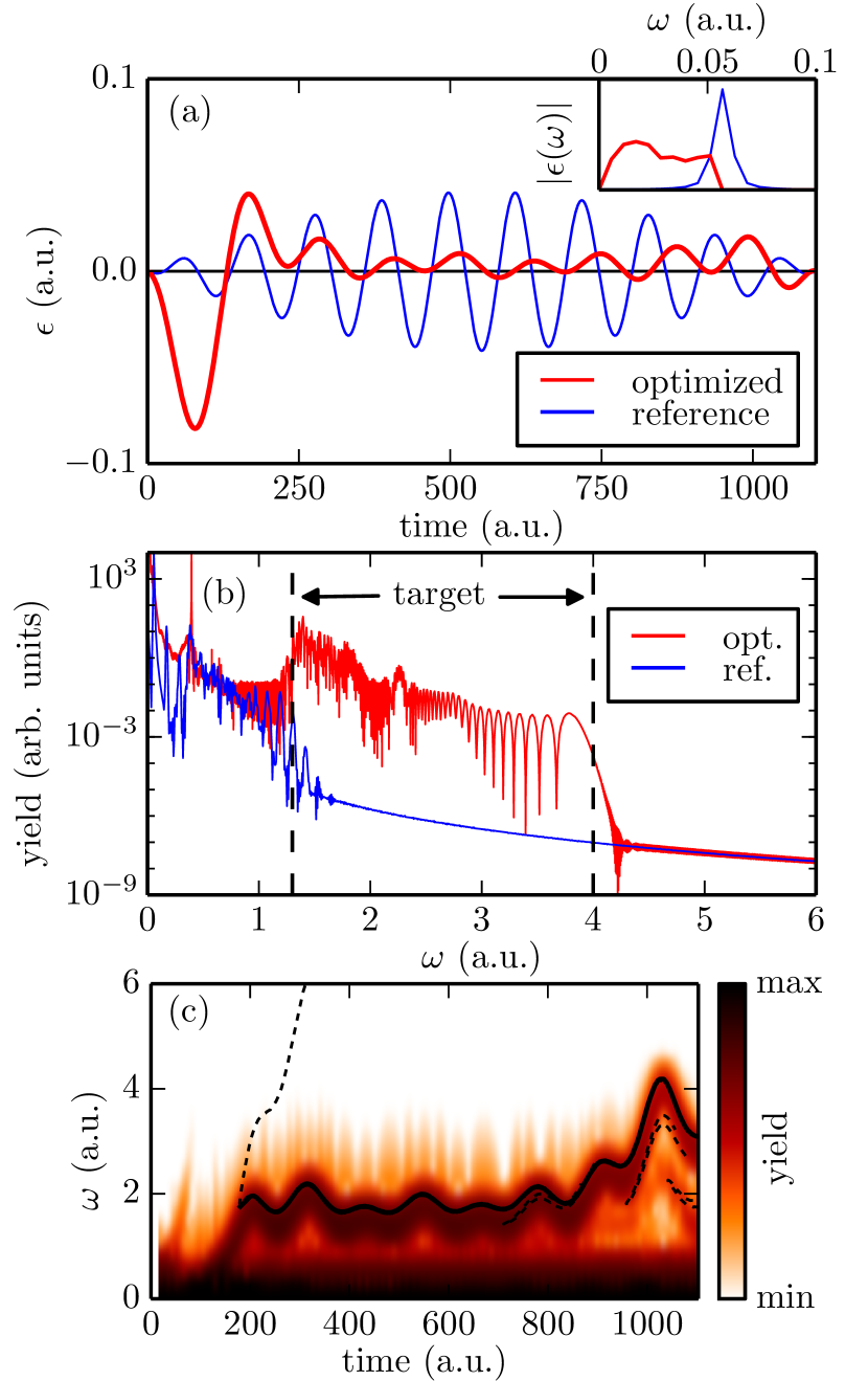
Figure 1: Optimization results for the HHG spectrum with the target range $\omega\in\left[1.3,4\right]$ a.u. The pulse length is $T=1104$ a.u. and the frequency of the reference pulse is $\omega=0.0569$ a.u., equal to the maximum frequency in the optimization. The fluence is kept constant. (a) Optimized [red (light gray)] and reference [blue (dark gray)] pulses and their frequencies (inset). (b) High-harmonic spectra for optimized [red (light gray) and reference [blue (dark gray)] pulses. The target range is shown with vertical dashed lines. (c) Quantum mechanical time-dependent harmonic spectrum in log-scale [colorscale (grayscale)] and return energies calculated from the semiclassical model (solid line). Spurious branches from uniform tunneling rate are shown with dashed lines (see text).

First we apply the Newuoa algorithm to optimize a laser pulse for HHG in the target interval $\omega\in\left[1.3,4\right]$ a.u. The pulse length is fixed to $T=1104$ ($26.7$ fs) and the carrier frequency of the reference pulse is $\omega=0.0569$ a.u. (wavelength $\lambda\approx 800$ nm corresponding to the typical range of Ti:sapphire lasers), which we choose to keep as the maximum allowed frequency of the optimized pulse to prevent the formation of complicated pulses with high frequency components. The peak intensity of the reference pulse is $6\times 10^{13}\,\text{W}/\text{cm}^{2}$, and the fluence is kept constant in the optimization. The reference and optimized pulses are shown in Fig. 1(a) as red (light gray) and blue (dark gray) lines, respectively. The optimized harmonic spectrum in Fig. 1(b) completely fulfills the desired target, and in addition to the cutoff extension, the yield is also increased by several orders of magnitude.

Next we comment on the two most obvious characteristics of the optimized pulse in Fig. 1(a). First, it is important to note that the high-intensity half-cycle in the beginning is not responsible for the significant increase in the HHG yield and cutoff. If this part were later in the pulse, the cutoff would be at $\omega\approx 2.5$ a.u. A similar effect is seen if, e.g., the last low-intensity peak is missing. Secondly, as shown in the inset of Fig. 1(a), the optimized pulse contains lower-frequency components. Indeed, the standard theoretical HHG considerations predict that lower frequencies should lead to higher cutoff energy due to higher ponderomotive energy. However, merely using low frequency single-color pulses produces very low yields. It is the shaped multi-frequency pulses that produce both the large cutoff and high intensities. Furthermore, in the case of HHG resulting from pulses that have a single carrier frequency, the harmonic peaks are equally separated by twice the carrier frequency. In the case of optimized pulses, however, we find no connection between the frequency components in the pulse and the HHG peak separations. This is expected in view of the complexity of the optimized pulse in the time-frequency plane, even though we applied rather simple pulse constraints as explained above.

The emission process is further demonstrated in Fig. 1(c), where the color (grayscale) image shows the time-frequency map of the quantum dipole acceleration, $\ddot{d}(t,\omega)$. The time-frequency map is calculated as a discrete short-time Fourier transform Allen (1977) (STFT) using the Blackman window function Blackman and Tukey (1958). In essence, the time-axis is split into multiple overlapping windows, and the dipole acceleration is Fourier-transformed in each window. Finally, we plot the quantity $S(t,\omega)=|\ddot{d}(t,\omega)|^{2}/\omega^{2}$ in log-scale in analog with the harmonic yield; here $t$ corresponds to the middle of each time-window of the STFTs. $S(t,\omega)$ essentially describes HHG in time. Bicubic interpolation is used for slight visual improvements. The cutoff extension up to $\omega\lesssim 2.5$ a.u. occurs throughout the pulse as it is the effect of the high-intensity peak. The full extension up to $\omega=4$ a.u., however, occurs only at the end of the pulse. This clarifies the above-mentioned fact that the complete structure of the optimized pulse is important.

Next we examine the physical origin of the cutoff extension in more detail by employing semiclassical simulations. An ensemble of classical trajectories is propagated with initial times $t_{0}$ distributed according to either a uniform tunneling rate $w(t_{0})\sim 1$ or exponential tunneling rate Perelomov et al. (1966); *[English:]PPTen; Ammosov et al. (1986); *[English:]ADKen; Delone and Krainov (1991) $w\left(t_{0}\right)\sim\exp\left\{-\Big{[}2\left(2I_{p}\right)^{3/2}\Big{]}/\Big{[}3\lvert\epsilon(t_{0})\rvert\Big{]}\right\}$, where $I_{p}=0.669$ a.u. is the ionization potential of our system. At the tunnel exit obtained from the classical turning point equation $V\left(x\right)+F_{x}\left(t\right)x=-I_{p}$, the velocity is set to zero and the electron is propagated classically. Upon return of the tunneled electron to the origin, a photon is emitted with frequency corresponding to the kinetic energy of the electron; also later returns are recorded and taken into account. Note that in contrast to the three-step (simple man) model Corkum (1993), where the electron starts from the origin and moves in the laser field only, the electron in our model starts at the tunnel exit and moves in the combined force field of the laser and the atomic potential. It should be noted that in contrast to our semiclassical simulation taking the atomic potential into account, the three-step model underestimates the cutoff energy. For the parameters of Fig. 2 the cutoff calculated from the three-step model corresponds to 3.2 a.u. (cf. to 4.2 a.u. predicted by semiclassical simulations with binding potential shown in Fig.2).

The return energy maps of the semiclassical model as a function of the return time (solid curves) are compared with the time-dependent harmonic spectrum in Fig. 1(c). Due to the pulse shape, the electron can return only once to the origin. With uniform tunneling distribution, the semiclassical model exhibits a few spurious branches (dashed black curves), which are suppressed when using the exponential tunneling rate. The remarkable agreement between the semiclassical and quantum descriptions highlights the classical origin of the cutoff extension.

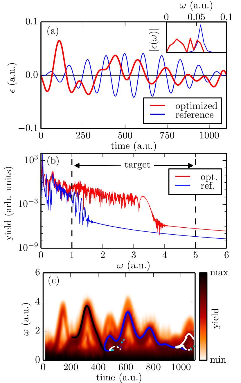
Figure 2: Same as Fig. 1 but for an extended target range (up to $\omega=5$ a.u.) and for the gradient-based BGFS optimization algorithm. In (c), energies of an electron calculated from the semiclassical model upon its first, second, third, and fourth return to the origin are shown with black, blue (medium gray), white, and cyan (light gray) curves, respectively.

In Fig. 2(a) we show a BFGS-optimized pulse [red (light gray)] with the same reference pulse [blue (dark gray)] as in Fig. 1. The target range is now $\omega\in\left[1,5\right]$ a.u., i.e., considerably larger than in the previous case. Despite a slightly more complicated temporal shape of the optimized pulse, the resulting HHG spectrum [Fig. 2(b)] is similar to the first case. Now, however, the optimized pulse allows multiple returns of the electron to the origin as shown in Fig. 2(c) when using an exponential tunneling rate. Not all of the quantum mechanical harmonic emissions can be found in the semiclassical model with exponential tunneling distribution. They are, however, allowed by the semiclassical model and visible when using a uniform tunneling rate. Therefore, the semiclassical picture does agree with the quantum description, but the exponential tunneling distribution does not produce all tunneling events.

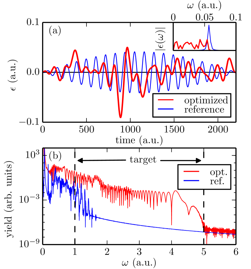
Figure 3: Same as Fig. 2(a-b) but for a longer pulse with $T=2209$ a.u. ($53.5$ fs).

Next we double the pulse length while keeping the peak intensity of the reference pulse, the maximum frequency, and the target HHG range the same (note that the fluence is also doubled). The BFGS-optimized pulse of Fig. 3(a) now leads to complete extension of the cutoff all the way up to $\omega=5$ a.u. as demonstrated in Fig. 3(b). This is likely due to higher fluence and more freedom in the shaping of the longer pulse.

The effect of late returns [see, e.g., Fig. 2(c)] can be analyzed in the semiclassical picture. The harmonic spectrum can be calculated as a histogram of the electron energies upon return to the origin with weights from the exponential tunneling rate (see above). The resulting spectra demonstrate varying contributions of late returns between different pulses. Even in the case of pulse of Fig. 2(a), where late returns are evident, their contributions to the spectra in the semiclassical models are minimal. In contrast, for the optimal pulse of Fig. 3, also the second return plays an important role in enhanced HHG.

The yield increase can be attributed to the increased tunneling probability compared to the reference pulses. Indeed, yield increase of comparable, albeit slightly larger, magnitude can be found when using single-frequency pulses with the same maximum amplitude as in the optimized pulses, but the extension of the cutoff does not reach the optimized results. Sensitivity of HHG to the pulse amplitude has been previously reported in, e.g., Refs. Kim et al. (2005) and Dahlström et al. (2011). The sensitivity is also obvious from the analytic factorization of the HHG rates in Ref. Frolov et al. (2009). We emphasize that the yield increase of the presented optimized HHG arises from increased tunneling rate, not from resonances as, e.g., in Ref. Ishikawa (2003): in our case a minimum of seven-photon absorption would be required, which is highly unlikely.

Finally, we verify which stationary states are involved in the enhanced HHG process. For this purpose, we solve the time-dependent Schrödinger equation in momentum space and velocity gauge by expanding the state in terms of the eigenstates of the field-free Hamiltonian Shvetsov-Shilovski et al. (2014). Note that the occupations are gauge-dependent. We find that approximately four lowest bound states are essential for the enhanced HHG, but ten are required for (nearly) full convergence of the spectrum; the numbers are similar for reference pulses. However, in the optimized HHG much of the electron density reaches high-energy continuum states, whereas the for the reference pulse the electron occupation is mostly in the bound states and in the low-energy continuum (see Fig. 4).

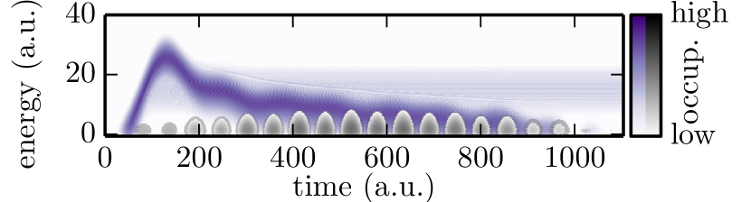
Figure 4: Occupations (log-scale) of stationary states in velocity gauge for the reference (gray bulb-shaped structures at the bottom) and optimized (colored structures elsewhere) pulse of Fig. 1.

To summarize, we have developed an optimal-control scheme to simultaneously enhance both the yield and the cutoff energy of high-harmonic generation (HHG). Our target functional, an integral over the harmonic yield in a desired energy range, leads to significant increase in the HHG yield and cutoff energy within two different optimization algorithms. Furthermore, we have shown through semiclassical studies that the extension of the cutoff is of classical origin. Instead, the increase in the harmonic yield is found to be due to increased tunneling probability arising from increased peak amplitudes, while the fluence is kept constant in the optimization. We note that in higher dimensional models, the harmonic yield will be affected by transversal spreading of the electron wave packet. However, our preliminary results (not shown here) demonstrate even the 1D-optimized pulses to provide qualitatively similar cutoff extension and no significant loss of yield also when applied to a two-dimensional model; we expect similar tendency also for three dimensions. In addition, by doing the optimization within the same dimensionality, there can be additional degrees of freedom in the pulse regarding, e.g., polarization, number of frequency components and pulse sources, which will help counter the issue of wave packet spreading.

We leave the detailed analysis of realistic pulse constraints to three-dimensional and many-electron models, where such analysis will be more relevant. With such refinements, we expect our method to be usable also in experimental applications, which can have direct implications in the development of efficient, flexible, and tunable light-emitting tabletop devices.