Optical bistability of graphene in the terahertz range

Abstract

We use an exact solution of the relaxation-time Boltzmann equation in an uniform AC electric field to describe the nonlinear optical response of graphene in the terahertz (THz). The cases of monolayer, bilayer and ABA-stacked trilayer graphene are considered, and the monolayer species is shown to be the most appropriate one to exploit the nonlinear free electron response. We find that a single layer of graphene shows optical bistability in the THz range, within the electromagnetic power range attainable in practice. The current associated with the third harmonic generation is also computed.

I Introduction

Optical bistability is a way of controlling light with light Gibbs ; Shen82 . Bistability refers to an optical effect where a system exhibits two different values of the transmitted light intensity for a single value of the input intensity. One way of analyzing the bistability is to explore the optical Kerr-effect, a non-linear phenomenon where the light the modulates material’s refractive index Boyd . In general, for the effect to be measurable, the light field must transverse a macroscopic distance within the non-linear material. In a semiconductor, optical bistability was observed a long time ago Gibbs79 . The desired goal in the field of optical bistability is the possibility of realizing in a single device a set of functionalities, such as switching, logic functions, memory with a fast time response, and modulation, all using a low power laser Almeida04 . Eventually, the practical realisation of an optical computer is in the horizon Smith85 .

In general, optical bistability can be realized at the interface between a linear and a non-linear material, with the reflected light intensity showing hysteresis Smith79 . However, what may seem surprising is that the hysteresis can be observed in a system one-atom thick, such as graphene. In the optical region of the spectrum, it has been shown that graphene has a strong non-linear optical response Hendry10 ; Gu12 ; Kim12 ; Mikhailov12 . The same phenomenon has been observed in graphene derivatives Liaros13 and in graphene nano-ribbons intercalated with boron nitride Zhang14 . It has also been shown that graphene can dramatically change the nonlinear response of a silicon photonic crystal Kim12 .

Theoretically, the non-linear response of graphene at optical frequencies has been exploited to produce a novel class of nonlinear self-confined modes Nesterov . On the other hand, in the THz spectral range, graphene has the potential for many applications Bludov2013 ; Low14 ; Abajo14 ; Stauber14 .

Some aspects of the non-linear optical properties of graphene have already been considered in the literature Mikhailov_2007 ; Mikhailov_2008 ; Mikhailov_2008_b ; Mikhailov_2009 . However, the exploitation of those properties to the problem of bistability was not considered before. Results for the non-linear Drude response of graphene in the collisionless regime have been derived previously Mikhailov_2007 ; Mikhailov_2008 ; Mikhailov_2008_b ; Mikhailov_2009 . Here we extend the derivation to the regime where a finite relaxation time exists, given two alternative methods to generate the expansion (one of them non-perturbative). The response of graphene to an electromagnetic pulse has also been obtained Mikhailov_2008_b . It has also been shown that strong magnetic fields, which drive the system to the quantum Hall regime, can induce a giant optical non-linearity in graphene Yao_2012 . In addition, the latter authors, have also discussed an efficient nonlinear generation of THz plasmons in graphene Yao_2014 .

In this paper we show that graphene has a strong non-linear response in the THz leading to the phenomenon of bistability. This property may allow the fabrication of active devices in this spectral range. Furthermore, the study of non-linear surface plasmon polaritons on graphene becomes accessible, since we can now solve the dispersion relation in the presence of a field-dependent conductivity. Indeed, one can even envision controlling light with light exploiting plasmonic nanostructures Martti12 .

The article is organized as follows. In Sec. II we present the general solution of the Boltzmann equation, which is exact within the momentum-independent relaxation time approximation. This solution is used in Sec. III to calculate the frequency-dependent nonlinear conductivity of monolayer, bilayer, and ABA-stacked trilayer graphene. The THz optical bistability in monolayer graphene is considered in Sec. IV and the last section is devoted to conclusions.

II Boltzmann equation for a 2D electron system under AC electric field

In the presence of an AC field, $\mathbf{E}=E(t)\mathbf{u}_{x}$ (which is directed along $x$-axis and the time dependence of $E(t)$, in principle, can have an arbitrary form), within the relaxation time approximation, the Boltzmann equation reads:

$$\frac{\partial f_{n}({\mathbf{k}},t)}{\partial t}-\frac{e}{\hbar}E(t)\frac{\partial f_{n}({\mathbf{k}},t)}{\partial k_{x}}=-\frac{f_{n}({\mathbf{k}},t)-f_{0}[\epsilon_{n}(\mathbf{k})]}{\tau}\,,$$ (1)

where $f_{0}[\epsilon_{n}(\mathbf{k})]$ is the Fermi-Dirac distribution function, $\epsilon_{n}(\mathbf{k})$ is the $n$-th band energy of 2D electrons with ${\mathbf{k}}=(k_{x},k_{y})$, and $\tau$ is the (microscopic) relaxation time. As shown in Appendix A, this equation can be solved analytically if we assume that the microscopic relaxation time does not depend on $\mathbf{k}$. Although it might look unrealistic at first sight, this approximation is justified by the fact that $\tau$ disappears from the expression for the electric current in the physically interesting limit of frequencies ($\omega\tau\gg 1$), as it will be shown below. Alternatively, one can solve Eq. (1) by iterations (see Appendix B), a procedure that allows to take into account the dependence of the microscopic relaxation time upon the electron momentum. The exact solution is:

$$f_{n}(\mathbf{k},t)=e^{-t/\tau}\int_{-\infty}^{t}\frac{dt^{\prime}}{\tau}e^{t^{\prime}/\tau}f_{0}[\epsilon(k_{x}+\kappa(t,t^{\prime}),k_{y})]\,.$$ (2)

Here we introduced a shorthand notation $\kappa(t,t^{\prime})=(e/\hbar)\int^{t}_{t^{\prime}}E(t^{\prime\prime})dt^{\prime\prime}$. For a harmonic time-dependence $E(t)=E_{0}\cos(\omega t)$, which will be focus of our study, the function $\kappa$ is

$$\kappa(t,t^{\prime})=\int^{t}_{t^{\prime}}\frac{eE(t^{\prime\prime})}{\hbar}dt^{\prime\prime}=\frac{eE_{0}}{\hbar\omega}[\sin(\omega t)-\sin(\omega t^{\prime})]\,.$$ (3)

III Non-linear current response

III.1 General expression

The current is given in terms of the solution of the Boltzmann equation, Eq. (2), by

$$j_{x} = -\frac{e}{\pi^{2}\hbar}\sum_{n=1}^{N}\int d\mathbf{k}\frac{\partial\epsilon_{n}}{\partial k_{x}}\,f_{n}(\mathbf{k},t)$$ (4)

$$= -\frac{e}{\pi^{2}\hbar}e^{-t/\tau}\int^{t}_{-\infty}\frac{dt^{\prime}}{\tau}e^{t^{\prime}/\tau}$$

$$\times\sum_{n=1}^{N}\int d\mathbf{k}\frac{\partial\epsilon_{n}}{\partial k_{x}}f_{0}[\epsilon_{n}(k_{x}+\kappa(t,t^{\prime}),k_{y})]\,,$$

where $N$ is the number of bands in the spectrum (e.g. 2 in the case of bilayer graphene) and the integration is over the first Brillouin zone. In the low temperature limit ($T\rightarrow 0$) the equilibrium Fermi-Dirac distribution function can be replaced by the Heaviside step-function $\theta$, so that the non-equilibrium distribution function becomes:

$$f_{0}[\epsilon_{n}(k_{x}+\kappa(t,t^{\prime}),k_{y})]=\theta[\epsilon_{F}-\epsilon_{n}(k_{x}+\kappa(t,t^{\prime}),k_{y})].$$ (5)

In the following, Eqs.(4–5) will be used to compute the non-linear response in different forms of graphene where the electronic energy spectra are different.

III.2 Monolayer graphene

The spectrum of monolayer graphene consists of only one band ($N=1$), which in the Dirac cone approximation can be respresented as $\epsilon_{1}(\mathbf{k})=v_{F}\hbar\sqrt{k_{x}^{2}+k_{y}^{2}}$ ($v_{F}=\sqrt{3}at/(2\hbar)$ is the Fermi velocity of the electrons, $a$ is the lattice constant and $t$ is the tight-binding nearest-neghbour hopping parameter). To compute $j_{x}$ we first focus our attention on the momentum integration. To that end, we define the integral

$$I_{11}(\kappa)=\int dk_{x}dk_{y}\frac{k_{x}}{\sqrt{k_{x}^{2}+k_{y}^{2}}}\theta\left(\epsilon_{F}-v_{F}\hbar\sqrt{(k_{x}+\kappa)^{2}+k_{y}^{2}}\right)\,,$$ (6)

such that

$$j_{x}=-\frac{ev_{F}}{\pi^{2}}e^{-t/\tau}\int^{t}_{-\infty}\frac{dt^{\prime}}{\tau}e^{t^{\prime}/\tau}I_{11}(\kappa),$$ (7)

and $\kappa\equiv\kappa(t,t^{\prime})$. Note that we consider a doped graphene sheet, i.e., we assume a finite $\epsilon_{F}$ (and a corresponding finite $k_{F}=\epsilon_{F}/(\hbar v_{F})$). Performing the substitutions $k_{x}+\kappa=\tilde{k}_{x}$, $k_{y}=\tilde{k}_{y}$ the integral becomes

$$I_{11}(\kappa)=\int d\tilde{k}_{x}d\tilde{k}_{y}\frac{\tilde{k}_{x}-\kappa}{\sqrt{(\tilde{k}_{x}-\kappa)^{2}+\tilde{k}_{y}^{2}}}\theta(\epsilon_{F}-v_{F}\hbar\sqrt{\tilde{k}_{x}^{2}+\tilde{k}_{y}^{2}})\,.$$ (8)

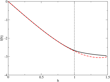
Figure 1: (color online) Plot of the function $I(\kappa)$ vs $h=\kappa/k_{F}$. Function $I(\kappa)$, as computed from Eq. (10), and (dashed line) the approximation given by Eq. (12); we have taken $k_{F}=1$.

Introducing the limits of integration imposed by the step-function, the integral splits into two terms

$$I_{11}(\kappa)=\int_{-k_{F}}^{k_{F}}d\tilde{k}_{y}\int_{0}^{\sqrt{k_{F}^{2}-k_{y}^{2}}}d\tilde{k}_{x}\frac{\tilde{k}_{x}-\kappa}{\sqrt{(\tilde{k}_{x}-\kappa)^{2}+\tilde{k}_{y}^{2}}}+$$

$$\int_{-k_{F}}^{k_{F}}d\tilde{k}_{y}\int^{0}_{-\sqrt{k_{F}^{2}-k_{y}^{2}}}d\tilde{k}_{x}\frac{\tilde{k}_{x}-\kappa}{\sqrt{(\tilde{k}_{x}-\kappa)^{2}+\tilde{k}_{y}^{2}}}\,.$$ (9)

The integral over $d\tilde{k}_{x}$ is elementary and we end up with

$$I_{11}(\kappa) = 2\int_{0}^{k_{F}}d\tilde{k}_{y}\left(\sqrt{\kappa^{2}+k_{F}^{2}-2\kappa\sqrt{k_{F}^{2}-\tilde{k}_{y}^{2}}}\right.$$ (10)

$$-\left.\sqrt{\kappa^{2}+k_{F}^{2}+2\kappa\sqrt{k_{F}^{2}-\tilde{k}_{y}^{2}}}\right)\,.$$

We note that $I_{11}(\kappa)$ is an odd function of $\kappa$. The integral $I_{11}(\kappa)$ can be written in terms of elliptic integrals, a result valid for all values of the ratio $\kappa/k_{F}$. In the regime $\kappa/k_{F}\leq 1$ the integral $I(\kappa)$ can be expressed in terms of the Gaussian hypergeometric functionAbramowitz ${}_{2}F_{1}(a,b;c,x)$ as

$$I_{11}(\kappa)=-\pi\kappa k_{F}\times\,_{2}F_{1}\left(-\frac{1}{2},\frac{1}{2};2,\frac{\kappa^{2}}{k_{F}^{2}}\right)\,.$$ (11)

Although this is a formal analytical expression, it is preferable to expand it in powers of $\kappa/k_{F}$,

$$I_{11}(\kappa)\approx-\pi k_{F}\kappa\left[1-\frac{1}{8}\left(\frac{\kappa}{k_{F}}\right)^{2}-\frac{1}{64}\left(\frac{\kappa}{k_{F}}\right)^{4}\right]\,.$$ (12)

It is important to stress that all terms but the first in this series have the same sign. A comparison between the result of Eq. (10) with the approximate expression (12) is given in Fig. 1. Clearly, the expansion (12) works very well all the way from $\kappa/k_{F}=0$ till $\kappa/k_{F}=1$.

To evaluate the current at zero temperature we still need to compute the integral over $t^{\prime}$. The first-order term is

$$J^{(1)} = e^{-t/\tau}\int^{t}_{-\infty}\frac{dt^{\prime}}{\tau}e^{t^{\prime}/\tau}\kappa(t,t^{\prime})$$ (13)

$$=\frac{eE_{0}}{\hbar}\frac{\tau[\cos(t\omega)+\tau\omega\sin(t\omega)]}{1+\tau^{2}\omega^{2}}$$

$$=\frac{eE_{0}}{2\hbar}\tau\frac{1+i\tau\omega}{1+\tau^{2}\omega^{2}}e^{-i\omega t}+{\rm c.c.}\,.$$

The current is thus

$$j_{x}^{(1)}=\frac{ev_{F}k_{F}}{\pi}J^{(1)}=\frac{e^{2}}{\pi\hbar}\frac{\epsilon_{F}\tau}{\hbar}\frac{1}{1-i\tau\omega}\frac{E_{0}}{2}e^{-i\omega t}\,,$$ (14)

which is nothing but Drude’s result. Here we have extracted the dependence of the integral on $e^{-i\omega t}$ only. In the limit $\omega\tau\gg 1$, the linear part of the current can be expressed as

$$j_{x}^{(1)}=i\nu_{1}\frac{E_{0}}{2}e^{-i\omega t}\,,\qquad\nu_{1}=\frac{e^{2}}{\pi\hbar}\frac{\epsilon_{F}}{\hbar\omega}\>.$$ (15)

The calculation of the third order term is more tedious.note1 We have to evaluate

$$J^{(3)}=e^{-t/\tau}\int^{t}_{-\infty}\frac{dt^{\prime}}{\tau}e^{t^{\prime}/\tau}\kappa^{3}(t,t^{\prime})=$$

$$-\frac{18\tau^{3}}{(2i\tau\omega-1)(1+\tau^{2}\omega^{2})}\left(\frac{eE_{0}}{2\hbar}\right)^{3}e^{-i\omega t}$$ (16)

$$+\frac{6\tau^{3}}{1-6i\omega\tau-11\tau^{2}\omega^{2}+6i\tau^{3}\omega^{3}}\left(\frac{eE_{0}}{2\hbar}\right)^{3}e^{-i3\omega t}+{\rm c.c.}\,$$

which for $\omega\tau\gg 1$ leads to

$$J^{(3)}=\frac{9i}{\omega^{3}}\left(\frac{eE_{0}}{2\hbar}\right)^{3}e^{-i\omega t}-\frac{i}{\omega^{3}}\left(\frac{eE_{0}}{2\hbar}\right)^{3}e^{-i3\omega t}\,.$$ (17)

The third order current, $j_{x}^{(3)}$, is given by

$$j_{x}^{(3)}=-\frac{ev_{F}}{8\pi k_{F}}J^{(3)}=j_{x}^{(3,\omega)}+j_{x}^{(3,3\omega)}\,,$$ (18)

where

$$j_{x}^{(3,\omega)}=-i\nu_{3}\frac{E_{0}^{3}}{8}e^{-i\omega t}\,,\qquad\nu_{3}=9\frac{e^{2}}{\hbar\pi}\frac{v_{F}^{2}}{8\epsilon_{F}}\frac{e^{2}}{\hbar\omega^{3}}$$ (19)

and

$$j_{x}^{(3,3\omega)}=i\frac{\nu_{3}}{9}\frac{E_{0}^{3}}{8}e^{-i3\omega t}\,.$$ (20)

The term $j_{x}^{(3,3\omega)}$ represents the third harmonic generation. We also note that result (19) differs by a factor of 3 from the result for the same quantity computed by Mikhailov Mikhailov_2007 . This difference exists, because Mikhailov treatment does not permit to study the regime of $\omega\tau\gg 1$, since by construction it assumes that the observation time is much smaller than $\tau$. Finally, the current to fifth order (in the limit $\tau\omega\gg 1$) is given by

$$j_{x}^{(5,\omega)}=-i\nu_{5}\left(\frac{E_{0}}{2}\right)^{5}e^{-i\omega t}\,,\qquad\nu_{5}=\frac{25}{16}\frac{e^{2}}{\hbar\pi}\frac{v_{F}^{4}}{\epsilon_{F}^{3}}\frac{e^{4}}{\hbar\omega^{5}}.$$ (21)

This concludes the derivation of the nonlinear response of monolayer graphene. An alternative way to obtain the nonlinear current in monolayer graphene is presented in Appendix B, where the Boltzmann equation is solved by means of expansion of the nonlinear distribution function in powers of the electric field, while here the expansion was performed during the calculation of the current density. In both cases the dimensionless expansion parameter is $k_{0}/k_{F}$, where $k_{0}=eE_{0}/(\hbar\omega)$. The procedure is valid if $k_{0}/k_{F}<1$.

III.3 Bilayer and trilayer graphene

We next consider a AB-stacked graphene bilayer, whose spectrum consists of two parabolic bands ($N=2$) and can be represented asc:bilayer

$$\epsilon_{1}({\bf k})=\frac{v_{F}^{2}\hbar^{2}(k_{x}^{2}+k_{y}^{2})}{t_{\perp}}\>;$$ (22)

$$\epsilon_{2}({\bf k})=t_{\perp}+\frac{v_{F}^{2}\hbar^{2}(k_{x}^{2}+k_{y}^{2})}{t_{\perp}},$$ (23)

where $t_{\perp}$ is the hopping parameter between the layers. Substituting (22) and (23) into Eq. (4), we obtain the following expression for the current density:

$$j_{x}=-\frac{2ev_{F}^{2}\hbar}{\pi^{2}t_{\perp}}e^{-t/\tau}\int^{t}_{-\infty}\frac{dt^{\prime}}{\tau}e^{t^{\prime}/\tau}\left[I_{21}(\kappa)+I_{22}(\kappa)\right],$$ (24)

where $I_{2n}$ with $n=1,\>2$ are integrals analogous to $I_{11}$ defined in the previous section, and are evaluated in Appendix C. Substituting them into Eq. (24) and using Eq. (13) we obtain:

$$j_{x}=\frac{2e}{\pi\hbar}\left[\epsilon_{F}+\left(\epsilon_{F}-t_{\perp}\right)\theta\left(\epsilon_{F}-t_{\perp}\right)\right]J^{(1)}$$

$$=\frac{2e^{2}}{\pi\hbar^{2}}\left[\epsilon_{F}+\left(\epsilon_{F}-t_{\perp}\right)\theta\left(\epsilon_{F}-t_{\perp}\right)\right]\frac{E_{0}}{2}\tau\frac{1+i\tau\omega}{1+\tau^{2}\omega^{2}}e^{-i\omega t}.$$

(25)

It is interesting that, owing to its parabolic energy spectrum [Eqs. (22)–(23)], bilayer graphene is a purely linear system. If the Fermi level is below the interlayer hopping energy $t_{\perp}$, the conductivity is equal to twice the first order conductivity of monolayer graphene [compare Eqs. (25) and (14)]. For $\epsilon_{F}>t_{\perp}$, there is a correction to the conductivity due to the second band filling.

The spectrum of the ABA-stacked trilayer graphene consists of one Dirac-type and two parabolic bands,c:trilayer

$$\epsilon_{1}=\frac{\hbar^{2}v_{F}^{2}(k_{x}^{2}+k_{y}^{2})}{\sqrt{2}t_{\perp}}\>;$$ (26)

$$\epsilon_{2}=\hbar v_{F}\sqrt{k_{x}^{2}+k_{y}^{2}}\>;$$ (27)

$$\epsilon_{3}=\sqrt{2}t_{\perp}+\frac{\hbar^{2}v_{F}^{2}(k_{x}^{2}+k_{y}^{2})}{\sqrt{2}t_{\perp}}\>.$$ (28)

Substituting these relations into Eq. (4) and proceeding as before we obtain the following expression for the induced current:

$$j_{x}=\frac{e^{2}}{\pi\hbar^{2}}\left[3\epsilon_{F}+2\left(\epsilon_{F}-\sqrt{2}t_{\perp}\right)\theta\left(\epsilon_{F}-\sqrt{2}t_{\perp}\right)\right]\times$$

$$\frac{E_{0}}{2}\tau\frac{1+i\tau\omega}{1+\tau^{2}\omega^{2}}e^{-i\omega t}+j_{x}^{(3)}+j_{x}^{(5,\omega)}\>.$$ (29)

Here $j_{x}^{(3)}$, $j_{x}^{(5,\omega)}$ coincide with those defined by Eqs. (18) and (21), respectively. The main result is that, in contrast with the case of bilayer graphene, this material is a nonlinear medium alike monolayer graphene. However, the linear part of the induced current in this case is larger than for monolayer graphene, so we may say that its nonlinearity is relatively weaker.

We note that below we use the expressions for the non-linear optical response of graphene in the collisionless regime. This may be experimentally justified. In a previous experimental study Lee_2011 of the transmittance of graphene in the wavenumber range of $[30,1000]$ cm^-1, a relaxation rate of $\Gamma=95$ cm^-1 was found (see Fig. 3 of that reference). For the two frequencies considered below the product $\omega\tau=2\pi f\tau$ is $2.2$ and $1.1$ for the frequencies of $f=1$ THz and $f=0.5$ THz, respectively (see also Ref. Mak_2012, for different (smaller) values of $\Gamma$). Clearly these numbers are not in the in the regime $\omega\tau\gg 1$. However, these numbers are for large area CVD grown graphene, which is known to produce a low-mobility material. On the other hand, exfoliated graphene has mobilities that are more than one order of magnitude larger. In an experiment done in this type of graphene one would be in the regime $\omega\tau\gg 1$. Indeed, a recent theoretical calculationSule_2014 of the optical response of suspended graphene in the terahertz range, using ab-initio methods, yielded a value of $\Gamma=1/\tau\sim 0.8$ THz which leads to $2\pi f/\Gamma\sim 7.9$.

IV Bistability of monolayer graphene

We shall now discuss the possibility of optical bistability in graphene. To this end, we start by solving the scattering problem in the geometry defined by Fig. 2, where a graphene sheet, the non-linear medium, is located at $z=0$.

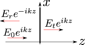
Figure 2: (color online) Scattering geometry. The thick line represents the graphene sheet.

The boundary conditions obeyed by the electromagnetic field are

$$E_{r}+E_{0}=E_{t}\,,$$ (30)

and

$$B_{L}-B_{R}=\mu_{0}j_{x}\,,$$ (31)

where $B_{L}$ is the magnetic field of the electromagnetic field to the left of graphene and $B_{R}$ that to the right. From Maxwell’s equations it follows that

$$\partial_{z}E_{x}=i\omega B_{y}\,,$$ (32)

which imply that

$$B_{L}=\frac{k}{\omega}(E_{0}-E_{r})\,,$$ (33)

and

$$B_{R}=\frac{k}{\omega}E_{t}\,.$$ (34)

Thus

$$\frac{k}{\omega}(E_{0}-E_{r})-\frac{k}{\omega}E_{t}=i\mu_{0}(\nu_{1}E_{t}-\nu_{3}E_{t}^{3}-\nu_{5}E_{t}^{5})\,,$$ (35)

or

$$E_{0}=E_{t}\left[1-i\frac{\mu_{0}c}{2}(\nu_{1}-\nu_{3}E_{t}^{2}-\nu_{5}E_{t}^{4})\right]\,,$$ (36)

where $\nu_{1}$, $\nu_{3}$, $\nu_{5}$ are defined in Eqs. (15), (19), and (21). We must stress the bistability effect does not require the inclusion of the fifth order term. We only include it here to show that the effect is not suppressed by higher order powers of the expansion. Here we suppose for convenience that $E_{t}$ is purely real, i.e. possesses zero phase, then $E_{0}$ is complex. Taking the square of the modulus of Eq. (36), we obtain

$$|E_{0}|^{2}=E_{t}^{2}\left[1+\frac{\mu_{0}^{2}c^{2}}{4}\nu_{1}^{2}\left(1-\frac{\nu_{3}+E_{t}^{2}\nu_{5}}{\nu_{1}}E_{t}^{2}\right)^{2}\right]\,.$$ (37)

Defining $|E_{0}|^{2}=Y$ and $E_{t}^{2}=X$ [Markos, ], we rewrite Eq. (37) as

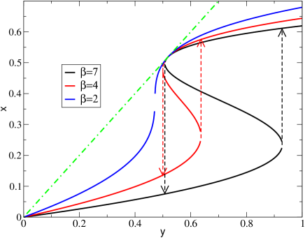
Figure 3: (color online) Bistability curves of the dimensionless field $x$ as function of $y$, for different values of the parameter $\beta$. When the power of the laser is increased the transmission through graphene follows the curve starting at zero until it reaches a point where the transmission suffers a sudden jump to higher values. The dashed-dotted straight line is the function $x=y$.

$$Y=X\left[1+\beta\left(1-\Lambda X\right)^{2}\right]$$ (38)

where

$$\beta=\frac{\mu_{0}^{2}c^{2}}{4}\nu_{1}^{2}=4\alpha^{2}\frac{\epsilon_{F}^{2}}{\hbar^{2}\omega^{2}}\,,$$ (39)

is a dimensionless parameter, $\alpha$ is the fine structure constant, and

$$\Lambda=\frac{\nu_{3}+E_{t}^{2}\nu_{5}}{\nu_{1}}=\frac{9}{8}\frac{v_{F}^{2}\hbar^{2}}{\epsilon_{F}^{2}}\frac{e^{2}}{\hbar^{2}\omega^{2}}+\frac{25}{16}\frac{v_{F}^{4}}{\epsilon_{F}^{4}}\frac{e^{4}}{\omega^{4}}X\,.$$ (40)

Clearly, it follows from Eq. (38) that for $X=1/\Lambda$ resonant transmission occurs, that is, the system becomes fully transparent ($X=Y$).note2

It is more convenient to rewrite Eq. (38) in dimensionless form. To that end we introduce the new variables

$$x=\frac{e^{2}E_{t}^{2}}{\hbar^{2}\omega^{2}k_{F}^{2}}$$ (41)

and

$$y=\frac{e^{2}E_{0}^{2}}{\hbar^{2}\omega^{2}k_{F}^{2}}\,,$$ (42)

which leads to a universal equation for the relation between $x$ and $y$ as function of the dimensionless parameter $\beta$:

$$y=x\left[1+\beta\left(1-\frac{9}{8}x-\frac{25}{16}x^{2}\right)^{2}\right]$$ (43)

Let us now analyse the consequences of Eq. (43). For a given value of $E_{0}$ this equation has one or more real solutions, such that $E_{t}<E_{0}$. These solutions are depicted in Fig. 3. From this figure we see that there is a region of incoming intensities ($Y_{-}\leq Y\leq Y_{+}$) for which there are three possible values of the transmitted intensity ($X$). However, the intermediate one corresponds to an unstable state (like in the case of first-order phase transitions). If one starts at small values of $Y$ and cranks up the intensity of the laser, one follows the lower curve till a point $Y_{+}$ where there is a sudden jump in the transmitted intensity $X$, represented by an arrow pointing up. On the other hand, if one starts at a high power and reduces it, the transmitted power will follow the solid curve, until it suddenly jumps to a regime of low transmission ($Y_{-}$), represented by a dashed line with an arrow pointing down. This implies that there is a hysteresis effect, or bistability. We should emphasize that this bistability is of electronic origin and, therefore, the switching of the bistability should be quite fast.

The incident power domain where Eq. (38) has three roots can be found by putting its discriminant equal to zero, namely

$$27\beta\Lambda^{2}Y^{2}-4\beta\Lambda(\beta+9)Y+4(1+\beta)^{2}=0\>$$ (44)

(the last term in (40) was neglected for simplicity). From Eq. (44) we obtain

$$Y_{\pm}=\frac{2}{27\beta\Lambda}\left[\beta(\beta+9)\pm\sqrt{\beta(\beta-3)^{3}}\right].$$ (45)

It follows from Eq. (45) that if $\beta\leq 3$ there is only one root of Eq. (38), i.e. there is no bistability. For $\beta>3$ an increase of $\beta$ leads to the broadening of the bistability domain $Y_{-}\leq Y\leq Y_{+}$.

The solution of the bistability equation in terms of dimensionless variables allow us to control the validity of the expansion, since for the considered parameters we always have $x<1$, that is, the condition $h=k_{0}/k_{F}<1$ [with $k_{0}=eE_{t}/(\hbar\omega)$] is not violated along the hysteresis curve.

V Conclusions

In summary, we analysed the nonlinear response of doped monolayer and multilayer graphene in the THz range, where it is determined by intraband transitions of free electrons. Our analysis, based on an exact solution of the relaxation-time Boltzmann equation, shows the crucial role of the Dirac-type electronic spectrum in getting considerable (third-order) nonlinearity and indicates monolayer graphene as the most appropriate one to exploit it. The nonlinearity causes the third harmonic generation (the current $j^{(3,3\omega)}$ calculated in Sec. III) and the optical bistability considered in the previous section. The latter is important because of its potential for applications in THz laser pulse modulation, optical switching, and signal processing. The estimated switching powers are attainable with existing terahertz radiation sources. In fact, THz lasers with peak electric fields of $\sim 4$ MV/m have recently been built Beck10 . Single-cycle THz pulses with amplitudes exceeding 100 MV/m are also possible Hirori11 . These peak values are within the range needed to perform experiments associated with the results of Fig. 3. The effect can be enhanced by stacking several layers of graphene together, separated from each other by a boron nitride spacer (rather than using multilayer graphene sheets).

Appendix A Exact solution of the Boltzmann equation

Here we give, for completeness, a derivation of the exact solution for the relaxation-time Boltzmann equation with uniform, time-dependent fields. This situation has been analyzed by a large number of researchers in the past. The solution is implicit (but not explicitly stated) in the early work of ChambersChambers , and analyzed in detail by Ignatov and Romanov in their discussion of nonlinear electromagnetic properties of semiconductor superlatticesIgnatov . To solve (1) we proceed as follows. Making the transformation

$$f({\mathbf{k}},t)=e^{-t/\tau}g(\mathbf{k},t)\,,$$ (46)

Eq.(1) reads

$$\tau\frac{\partial g({\mathbf{k}},t)}{\partial t}-k_{0}(t)\frac{\partial g({\mathbf{k}},t)}{\partial k_{x}}=f_{0}e^{t/\tau}\,,$$ (47)

where $k_{0}(t)=eE(t)\tau/\hbar$. This differential equation can be solved by the method of characteristics. We thus write

$$\frac{dt}{\tau}=-\frac{dk_{x}}{k_{0}(t)}=\frac{dg({\mathbf{k}},t)}{f_{0}e^{t/\tau}}\,.$$ (48)

The characteristic curves are defined by the solution of

$$\frac{dt}{\tau}=-\frac{dk_{x}}{k_{0}(t)}\Leftrightarrow k_{0}(t)dt=-\tau dk_{x}\,,$$ (49)

which upon integration gives

$$\int^{t}k_{0}(t_{1})dt_{1}+\tau k_{x}=C\,,$$ (50)

which defines a family of curves for different $C$’s. We can again use the characteristic relations and write

$$dg({\mathbf{k}},t)=f_{0}(k_{x},k_{y})e^{t/\tau}\frac{dt}{\tau}\,.$$ (51)

Using the equation for the characteristic curve we write

$$dg({\mathbf{k}},t)=f_{0}[C/\tau-\int^{t}k_{0}(t_{1})dt_{1}/\tau,k_{y}]e^{t/\tau}\frac{dt}{\tau}\,,$$ (52)

which upon integration gives

$$g({\mathbf{k}},t)=\int_{t_{0}}^{t}\frac{dt^{\prime}}{\tau}f_{0}[C/\tau-\int^{t^{\prime}}k_{0}(t_{1})dt_{1}/\tau,k_{y}]e^{t^{\prime}/\tau}\,,$$ (53)

and writing

$$C/\tau=\int^{t}k_{0}(t_{1})dt_{1}/\tau+k_{x}\,,$$ (54)

the equation for $g({\mathbf{k}},t)$ reads

$$g({\mathbf{k}},t)=\int_{t_{0}}^{t}\frac{dt^{\prime}}{\tau}e^{t^{\prime}/\tau}f_{0}[k_{x}+\int^{t}_{t^{\prime}}k_{0}(t_{1})dt_{1}/\tau,k_{y}]\,,$$ (55)

from which $f(\mathbf{k},t)$ follows. The value of $t_{0}$ is determined from the condition: if $k_{0}(t)\rightarrow 0$ then $f(\mathbf{k},t)\rightarrow f_{0}(\mathbf{k})$. In this limit we obtain

$$\lim_{E(t)\rightarrow 0}f(\mathbf{k},t)\rightarrow f_{0}(\mathbf{k})e^{-t/\tau}\int_{t_{0}}^{t}e^{t^{\prime}/\tau}dt^{\prime}/\tau\,,$$ (56)

which implies that $t_{0}=-\infty$. Thus

$$f(\mathbf{k},t)=e^{-t/\tau}\int_{-\infty}^{t}\frac{dt^{\prime}}{\tau}e^{t^{\prime}/\tau}f_{0}[k_{x}+\int^{t}_{t^{\prime}}k_{0}(t_{1})dt_{1}/\tau,k_{y}]\,,$$ (57)

the result presented in the main text.

Appendix B Iterative solution of the Boltzmann equation

The results obtained in the bulk of the text for the non-linear current can also be derived, although in a less elegant way, by an iterative approach. We give here the derivation of the current $j_{x}^{3,\omega}$ for the case of graphene. We assume a momentum independent relaxation time, but the method works as well if $\tau$ is momentum dependent.

Within the relaxation time approximation, Boltzmann equation reads

$$\frac{\partial f}{\partial t}-\frac{e}{\hbar}\vec{E}\cdot\vec{\nabla}_{\vec{k}}f=-\frac{f-f_{0}}{\tau}$$ (58)

where $e>0$, $f_{0}$ is the distribution function in equilibrium, and $f$ is the distribution function in the presence of the field (that it, out of equilibrium). We assume that the system is subjected to a finite AC field of the form

$$\vec{E}=\epsilon_{0}\hat{u}_{x}e^{-i\omega t}+\epsilon_{0}^{\ast}\hat{u}_{x}e^{i\omega t}\,,$$ (59)

where at some point in the calculation we take $\epsilon_{0}=\epsilon_{0}^{\ast}=E_{0}/2$. We seek a distribution function in the form

$$f(t)=f_{0}+f_{1}(t)+f_{2}(t)+f_{3}(t)\,,$$ (60)

where the sub-index refers to the power of the field within the term of the distribution.

We note in passing that the solution of a differential equation of the form

$$\dot{y}+ay=s(t)\,,$$ (61)

where $s(t)$ is a source term, reads

$$y(t)=e^{-at}\int_{-\infty}^{t}s(t^{\prime})e^{at^{\prime}}dt^{\prime}\,.$$ (62)

For sure, this is indeed a particular solution, but one where the memory of the transient response has been lost; this is assured by taking $t^{\prime}=-\infty$ in the lower limit of the integral. In the context of the response of an electron gas to an AC electric field, where dissipation exists, this choice for the lower limit of the integral is physically justified.

We now plug in the expansion (60) in Boltzmann equation and gather the terms with the same order in the field. This leads to

$$\dot{f}_{1}+\frac{f_{1}}{\tau} = \frac{e}{\hbar}\vec{E}\cdot\vec{\nabla}_{\vec{k}}f_{0}\,,$$ (63)

$$\dot{f}_{2}+\frac{f_{2}}{\tau} = \frac{e}{\hbar}\vec{E}\cdot\vec{\nabla}_{\vec{k}}f_{1}\,,$$ (64)

$$\dot{f}_{3}+\frac{f_{3}}{\tau} = \frac{e}{\hbar}\vec{E}\cdot\vec{\nabla}_{\vec{k}}f_{2}\,.$$ (65)

Equation (63) is of the form (62) and we obtain for $f_{1}$ the result

$$f_{1}=\frac{\partial f_{0}}{\partial\epsilon}\frac{e\vec{v}_{F}\cdot\hat{u}_{x}\epsilon_{0}}{1/\tau-i\omega}e^{-i\omega t}+\frac{\partial f_{0}}{\partial\epsilon}\frac{e\vec{v}_{F}\cdot\hat{u}_{x}\epsilon_{0}^{\ast}}{1/\tau+i\omega}e^{i\omega t}\,,$$ (66)

where $\epsilon=v_{F}\hbar k$ and $\vec{v}_{F}=v_{F}\vec{k}/k$. The details of the calculation are as follows:

$$f_{1}=e^{-t/\tau}\frac{e}{\hbar}\vec{\nabla}_{\vec{k}}f_{0}\cdot\int_{-\infty}^{t}(\epsilon_{0}\hat{u}_{x}e^{-i\omega t}+\epsilon_{0}^{\ast}\hat{u}_{x}e^{i\omega t})e^{t^{\prime}/\tau}dt^{\prime}\,.$$ (67)

Upon integration, the result (66) follows. We have also used the result

$$\vec{\nabla}_{\vec{k}}f_{0}=\frac{\partial f_{0}}{\partial\epsilon}\vec{v}_{F}\,.$$ (68)

We now proceed to the solution of equation (64). Explicitly, we have

$$\dot{f}_{2}+\frac{f_{2}}{\tau}=\frac{e}{\hbar}(\epsilon_{0}\hat{u}_{x}e^{-i\omega t}+\epsilon_{0}^{\ast}\hat{u}_{x}e^{i\omega t})\cdot\vec{\nabla}_{\vec{k}}\left[\frac{\partial f_{0}}{\partial\epsilon}\left(\frac{e\vec{v}_{F}\cdot\hat{u}_{x}\epsilon_{0}}{1/\tau-i\omega}e^{-i\omega t}+\rm{H.\,c.}\right)\right]$$ (69)

Taking $\epsilon_{0}=\epsilon_{0}^{\ast}$ and solving the differential equation, we obtain for $f_{2}$ the result

$$f_{2} = f_{0}^{\prime\prime}\frac{e^{2}v_{F}^{2}}{1/\tau-i\omega}(\vec{v}_{F}\cdot\hat{u}_{x}\epsilon_{0})^{2}\left(\frac{e^{-2i\omega t}}{1/\tau-2i\omega}+\tau\right)$$ (70)

$$+ f_{0}^{\prime}\frac{e^{2}v_{F}}{\/\tau-i\omega}\frac{1}{\hbar k}[\epsilon_{0}^{2}-(\epsilon_{0}\hat{u}_{x}\cdot\vec{v}_{F}/v_{F})^{2}]\left(\frac{e^{-2i\omega t}}{1/\tau-2i\omega}+\tau\right)+\rm{H.\,c.}\,,$$

where

$$f_{0}^{\prime}=\frac{\partial f_{0}}{\partial\epsilon}$$ (71)

and

$$f_{0}^{\prime\prime}=\frac{\partial^{2}f_{0}}{\partial\epsilon^{2}}\,,$$ (72)

and the result ($\vec{\epsilon}_{0}=\epsilon_{0}\hat{u}_{x}$)

$$\vec{\nabla}_{\vec{k}}(\vec{\epsilon}_{0}\cdot\vec{v}_{F})=v_{F}\vec{\nabla}_{\vec{k}}(\vec{\epsilon}_{0}\cdot\vec{k}/k)=v_{F}\left(\frac{\vec{\epsilon}_{0}}{k}-\frac{\vec{\epsilon}_{0}\cdot\vec{k}}{k^{3}}\vec{k}\right)$$ (73)

has been used. Clearly, $f_{2}$ does not contribute to the current, because

$$\int_{0}^{2\pi}\cos\theta=\int_{0}^{2\pi}\cos^{3}\theta=0\,.$$ (74)

We should note the presence in $f_{2}$ of a term that does not oscillate in time. This term, however, will contribute to another term in $f_{3}$ oscillating with frequency $\omega$. Finally, we have to solve

$$\dot{f}_{3}+\frac{f_{3}}{\tau}=\frac{e}{\hbar}(e^{-i\omega t}+e^{i\omega t})\epsilon_{0}\hat{u}_{x}\cdot\vec{\nabla}_{\vec{k}}f_{2}\,.$$ (75)

The rhs of the last equation together with its integration produces a number of terms. We are interested in those terms proportional to $e^{-i\omega t}$. We note that we can write $f_{2}$ in form more convenient to our purposes (that is, power counting) as

$$f_{2} = \left[f_{0}^{\prime\prime}e^{2}(\vec{v}_{F}\cdot\hat{u}_{x}\epsilon_{0})^{2}+f_{0}^{\prime}\frac{e^{2}v_{F}}{\hbar k}[\epsilon_{0}^{2}-(\epsilon_{0}\hat{u}_{x}\cdot\vec{v}_{F}/v_{F})^{2}]\right]$$

$$\times \left(\frac{2}{(1/\tau)^{2}+\omega^{2}}+\frac{e^{-2i\omega t}}{(1/\tau-i\omega)(1/\tau-2i\omega)}+\rm{H.\,c.}\right)\,,$$

where H. c. refers to the Hermitian conjugate of the second term. Given the form of $f_{3}$ in (75) and equation (LABEL:eq_f2_new_form) it is a simple task to isolate those terms proportional to $e^{-i\omega t}$; there are four such terms. The calculations are straightforward. The result is

$$f_{3} = \frac{e^{3}v_{F}^{2}}{\hbar}\epsilon_{0}\hat{u}_{x}\cdot\vec{\nabla}_{\vec{k}}[f_{0}^{\prime\prime}(\epsilon_{0}\hat{u}_{x}\cdot\vec{k}/k)^{2}]g(\omega)$$ (77)

$$+ \frac{e^{3}v_{F}}{\hbar^{2}}\epsilon_{0}\hat{u}_{x}\cdot\vec{\nabla}_{\vec{k}}[f_{0}^{\prime}(\epsilon_{0}^{2}/k-(\epsilon_{0}\hat{u}_{x}\cdot\vec{k})^{2}/k^{3})]g(\omega)$$

$$+ \ldots\,,$$

where $g(\omega)$ reads

$$g(\omega) = \frac{2}{1/\tau^{2}+\omega^{2}}\frac{e^{-i\omega t}}{1/\tau-i\omega}$$ (78)

$$+ \frac{e^{-i\omega t}}{(1/\tau-i\omega)^{2}(1/\tau-2i\omega)}\,.$$

In Eq. (77) only the terms proportional to $e^{-i\omega t}$ are written explicitly. The collisionless limit of $g(\omega)$ reads

$$\lim_{\tau\rightarrow\infty}g(\omega)=\frac{3i}{2\omega^{3}}e^{-i\omega t}\,.$$ (79)

We notice that the terms containing derivatives of the $\delta-$functions do not contribute to the current. In this case, the current that oscillates with frequency $\omega$ is simply given by

$$j^{(3,\omega)}_{x} = -\frac{e^{4}v_{F}}{\pi^{2}\hbar^{3}}\int_{0}^{2\pi}\int_{0}^{\infty}kdk\cos^{2}\theta\delta(k-k_{F})\frac{1}{k^{2}}\times$$ (80)

$$3\epsilon_{0}^{3}\sin^{2}\theta g(\omega)\,.$$

Performing the integrations and writing $\epsilon_{0}=E_{0}/2$ we obtain

$$j^{(3,\omega)}_{x}=-\frac{3}{4}\frac{e^{4}}{\pi\hbar^{3}}\frac{v_{F}}{k_{F}}\frac{E_{0}^{3}}{8}g(\omega)\,,$$ (81)

which in the collisionless limit reads

$$j^{(3,\omega)}_{x}=-i\frac{9}{8}\frac{e^{4}}{\pi\hbar^{3}}\frac{v_{F}}{k_{F}}\frac{E_{0}^{3}}{8}e^{-i\omega t}\,.$$ (82)

The explicit form of $f_{3}$ is obtained from

$$f_{3} = f_{0}^{\prime\prime\prime}e^{3}(\vec{\epsilon}_{0}\cdot\vec{v}_{F})^{3}g(\omega)+f_{0}^{\prime\prime}\frac{e^{3}}{\hbar}\vec{\epsilon}_{0}\cdot\vec{\nabla}_{\vec{k}}(\vec{v}_{F}\cdot\vec{\epsilon}_{0})^{2}g(\omega)$$ (83)

$$+ f_{0}^{\prime\prime}\frac{e^{3}}{\hbar}v_{F}\vec{v}_{F}\cdot\vec{\epsilon}_{0}\left(\frac{\epsilon_{0}^{2}}{k}-\frac{(\vec{\epsilon}_{0}\cdot\vec{k})^{2}}{k^{3}}\right)g(\omega)$$

$$+ f_{0}^{\prime}\frac{e^{3}}{\hbar^{2}}v_{F}\vec{\epsilon}_{0}\cdot\vec{\nabla}_{\vec{k}}\left(\frac{\epsilon_{0}^{2}}{k}-\frac{(\vec{\epsilon}_{0}\cdot\vec{k})^{2}}{k^{3}}\right)g(\omega)$$

$$+ \ldots\,,$$

where the following relations are useful

$$\vec{\epsilon}_{0}\cdot\vec{\nabla}_{\vec{k}}(\vec{\epsilon}_{0}\cdot\vec{v}_{F}/v_{F})^{2} = 2(\vec{\epsilon}_{0}\cdot\vec{v}_{F}/v_{F})\times$$ (84)

$$\left(\frac{\epsilon_{0}^{2}}{k}-\frac{(\vec{\epsilon}_{0}\cdot\vec{k})^{2}}{k^{3}}\right)$$

and

$$\vec{\epsilon}_{0}\cdot\vec{\nabla}_{\vec{k}}\left(\frac{\epsilon_{0}^{2}}{k}-\frac{(\vec{\epsilon}_{0}\cdot\vec{k})^{2}}{k^{3}}\right) = -3\frac{\epsilon_{0}^{2}}{k^{2}}(\vec{\epsilon}_{0}\cdot\vec{v}_{F}/v_{F})$$ (85)

$$+ 3\frac{(\vec{\epsilon}_{0}\cdot\vec{v}_{F}/v_{F})^{3}}{k^{2}}\,.$$

We also note the result

$$\int F(k)\delta^{(n)}(k-k_{F})dk=(-1)^{n}F^{(n)}(k_{F})\,,$$ (86)

where the superscript $(n)$ refers to the order of the derivative in order to $k$. This result is used to prove that the terms proportional to derivatives of the $\delta-$function (the first three terms) in Eq. (83) give a zero contribution to the current.

Appendix C Details of calculation of the current in bilayer and trilayer graphene

Two parabolic bands characteristic of bilayer graphene lead to the following integrals entering the expression for the current density (24):

$$I_{2n}(\kappa)=\int dk_{x}dk_{y}k_{x}\times$$

$$\theta\left\{\epsilon_{F}-\delta_{2,n}t_{\perp}-\frac{v_{F}^{2}\hbar^{2}\left[(k_{x}+\kappa)^{2}+k_{y}^{2}\right]}{t_{\perp}}\right\}\,,$$ (87)

In order to evaluate these integrals, we perform the same substitution as in the calculation of $I_{11}$, $k_{x}+\kappa=\tilde{k}_{x}$ and $k_{y}=\tilde{k}_{y}$. Thus, (87) takes the form

$$I_{2n}(\kappa)=\int d\tilde{k}_{x}d\tilde{k}_{y}(\tilde{k}_{x}-\kappa)\times$$

$$\theta\left(\epsilon_{F}-\delta_{2,n}t_{\perp}-\frac{v_{F}^{2}\hbar^{2}(\tilde{k}_{x}^{2}+\tilde{k}_{y}^{2})}{t_{\perp}}\right)$$

$$=-\kappa\pi\frac{\left(\epsilon_{F}-\delta_{2,n}t_{\perp}\right)t_{\perp}}{v_{F}^{2}\hbar^{2}}\theta\left(\epsilon_{F}-\delta_{2,n}t_{\perp}\right)\,.$$ (88)

In the case of trilayer graphene, the current density is:

$$j_{x}=-\frac{\sqrt{2}ev_{F}^{2}\hbar}{\pi^{2}t_{\perp}}e^{-t/\tau}\int^{t}_{-\infty}\frac{dt^{\prime}}{\tau}e^{t^{\prime}/\tau}\left[I_{31}(\kappa)+I_{33}(\kappa)\right]-$$

$$-\frac{ev_{F}}{\pi^{2}}e^{-t/\tau}\int^{t}_{-\infty}\frac{dt^{\prime}}{\tau}e^{t^{\prime}/\tau}I_{32}(\kappa),$$ (89)

where

$$I_{3n}(\kappa)=\int dk_{x}dk_{y}k_{x}\times$$

$$\theta\left\{\epsilon_{F}-\delta_{3,n}\sqrt{2}t_{\perp}-\frac{v_{F}^{2}\hbar^{2}\left[(k_{x}+\kappa)^{2}+k_{y}^{2}\right]}{\sqrt{2}t_{\perp}}\right\}\,.$$ (90)

for $n=1,3$ and $I_{32}(\kappa)=I_{11}(\kappa)$ [see Eq. (6)]. Using this and the similarity between the integrals $I_{31}$, $I_{33}$ and $I_{21}$, $I_{22}$ (replacing $t_{\perp}\to\sqrt{2}t_{\perp}$), we obtain the final expression for the current density given in the text.

References

- (1) Hyatt M. Gibbs, Optical Bistability: Controlling Light with Light, (Academic Press, 1985).
- (2) Y. R. Shen, Nature 299, 779 (1982)
- (3) R. W. Boyd, Nonlinear Optics, 3th. Ed., (Academic Press, 2008).
- (4) H. M. Gibbs, S. L. McCall, T. N. C. Venkatesan, A. C. Gossard, A. Passner, and W. Wiegmann, Appl. Phys. Lett. 35, 451 (1979).
- (5) Vilson R. Almeida and Michal Lipson, Optics Letters 29, 2387 (2004).
- (6) S. D. Smith, Nature 316, 319 (1985).
- (7) P. W. Smith, J.-P. Hermann, W. J. Tomlinson, and P. J. Maloney, Appl. Phys. Lett. 35, 846 (1979).
- (8) E. Hendry, P. J. Hale, J. Moger, A. K. Savchenko, and S. A. Mikhailov, Phys. Rev. Lett. 105, 097401 (2010).
- (9) S. A. Mikhailov, Physica E 44, 924 (2012).
- (10) T. Gu, N. Petrone, J. F. McMillan, A. van der Zande, M. Yu, G. Q. Lo, D. L. Kwong, J. Hone, and C. W. Wong, Nature Photonics 6, 554 (2012).
- (11) Kinam Kim, Seong-Ho Cho, and Chang-Won Lee, Nature Photonics 6, 502 (2012)
- (12) N. Liaros, A. B. Bourlinos, R. Zboril, and S. Couris, Optics Express 21, 21027 (2013).
- (13) Minyi Zhang, Guangshe Li, and Liping Li, J. Mater. Chem. C 2, 1482 (2014).
- (14) Maxim L. Nesterov, Jorge Bravo-Abad, Alexey Yu. Nikitin, Francisco J. Garc a-Vidal, and Luis Martin-Moreno, Laser Photonics Rev. 7, L7 (2013).
- (15) Yu. V. Bludov, A. Ferreira, N. M. R. Peres, and M. I. Vasilevskiy, Int. J. Mod. Phys. B 27, 1341001 (2013).
- (16) Tony Low and Phaedon Avouris, ACS Nano 8, 1086 (2014).
- (17) F. Javier Garcia de Abajo, ACS Photonics 1, 135 (2014).
- (18) T. Stauber, J. Phys. Condens. Matter 26, 123201 (2014).
- (19) S. A. Mikhailov, Europhys. Lett. 79, 27002 (2007).
- (20) S. A. Mikhailov and K. Ziegler, J. Phys.: Condens. Matter 20, 384204 (2008).
- (21) S.A. Mikhailov, Physica E 40, 2626 (2008).
- (22) S.A. Mikhailov, Microelectronics Journal 40, 712 (2009).
- (23) Xianghan Yao and Alexey Belyanin, Phys. Rev. Lett. 108, 255503 (2012).
- (24) Xianghan Yao, Mikhail Tokman, and Alexey Belyanin, Phys. Rev. Lett. 112, 055501 (2014).
- (25) Martti Kauranen and Anatoly V. Zayats, Nature Photonics 6, 737 (2012).
- (26) M. Abramowitz and I. Stegun, eds., Handbook of Mathematical Functions (Dover, New York, 1972).
- (27) Second order term vanishes since we consider a spatially homogeneous system. Electron convection current (dependent on coordinate), quadratic in electric field was considered in Ref. Popov2013, .
- (28) V. V. Popov, Appl. Phys. Lett. 102, 253504 (2013).
- (29) A. Ferreira, J. Viana-Gomes, J. Nilsson, E. R. Mucciolo, N. M. R. Peres, and A. H. Castro Neto, Phys. Rev. B 83, 165402 (2011).
- (30) Z. Rashidian, Yu. V. Bludov, N. M. R. Peres, and M. I. Vasilevskiy, arXiv:1402.7218 (2014).
- (31) Peter Markos and Costas M. Soukoulis, Wave Propagation: From Electrons to Photonic Crystals and Left-Handed Materials, (Princeton University Press, 2008).
- (32) Note that we are considering the regime where the physics is dominated by the intraband optical conductivity and therefore there is no relation between the so called universal conductivity of grapheneNair in the optical range, where graphene shows a transmittance of 97.7%, and the present regime of validity of our calculations, which apply to the THz range.
- (33) R. R. Nair, P. Blake, A. N. Grigorenko, K. S. Novoselov, T. J. Booth, T. Stauber, N. M. R. Peres, and A. K. Geim, Science 320, 1308 (2008).
- (34) Chul Lee, Joo Youn Kim, Sukang Bae, Keun Soo Kim, Byung Hee Hong, and E. J. Choi, Appl. Phys. Lett. 98 071905 (2011).
- (35) Kin Fai Mak, Long Ju, Feng Wang, and Tony F. Heinz, Solid State Communications 152, 1341 (2012).
- (36) N. Sule, K. J. Willis, S. C. Hagness, and I. Knezevic, Phys. Rev. B 90, 045431 (2014).
- (37) M. Beck, H. Schäfer, G. Klatt, J. Demsar, S. Winnerl, M. Helm, and T. Dekorsy, Optics Express 18, 9251 (2010).
- (38) H. Hirori, A. Doi, F. Blanchard, and K. Tanaka, Appl. Phys. Lett. 98, 091106 (2011).
- (39) R. G. Chambers, Proc. Phys. Soc. (London) Series A 65, 458 (1952).
- (40) A. A. Ignatov and Yu. A. Romanov, phys. stat. sol. (b) 78, 327 (1976).