Static corrections versus dynamic correlation effects
in the valence band Compton profile spectra of Ni

Abstract

We compute the Compton profile of Ni using the Local Density Approximation of Density Functional Theory supplemented with electronic correlations treated at different levels. The total/magnetic Compton profiles show not only quantitative but also qualitative significant differences depending weather Hubbard corrections are treated at a mean field +U or in a more sophisticated dynamic way. Our aim is to discuss the range and capability of electronic correlations to modify the kinetic energy along specific spatial directions. The second and the fourth order moments of the difference in the Compton profiles are discussed as a function of the strength of local Coulomb interaction $U$.

I Introduction

The study of physical and chemical properties of transition metals is still an extremely active experimental field and at the same time is the subject of extensive theoretical studies. The fascinating aspect of $d$-electron systems is the possible interplay of relativistic and electron correlation effects that has long been questioned. Ab-initio methods provide the framework in which relativity and correlations may be treated at equal footing. One notable example is the magnetic anisotropy energy for Ni. Experimentally it is known that the easy axis is along the [111] direction and the energy cost to rotate the magnetic moment axis into [001] direction is about $3~{}\mu$eV per atom[1]. LSDA+U calculations [2] accounting for spin-orbit and non-collinear coupling have been employed and showed to reproduce these values for relatively small value of the local Coulomb interaction $U=1.9$ eV and $J=1.2$ eV. Changes in the topology of the Fermi surface were discussed in the context of magneto-crystalline anisotropy of Ni [3]. These changes were recently addressed using the Gutzwiller variational theory with ab-initio parameters which showed the importance of the spin-orbit coupling [4].

As a matter of fact, nickel is perhaps the most studied electronic system. In the ordered ferromagnetic phase the vast majority of band structure calculations within the Local Density Approximation to the Density Functional Theory (DFT) converge to a value for the magnetic moment of $\approx 0.62~{}\mu_{B}$, which is a slightly overestimation of the experimental data. The orbital contribution amounts up to $10\%$ and the spin moment is found to be around $0.56~{}\mu_{B}$. The Generalized Gradient Approximation (GGA) add gradient correction to the local density approximation, does not change upon the value of the magnetic moment, however improve on the equilibrium lattice parameter and bulk modulus. The exchange splitting in both LSDA/GGA is in the range of $0.7$ to $0.75$ eV [5], while experimental data are situated between $0.3-0.5$ eV [6, 7, 8, 9, 10]. The valence band photoemission spectra of Ni shows a $3d$-band width that is about $30\%$ narrower than the value obtained from the LSDA calculations. It is known that LSDA cannot reproduce the dispersionless feature at about 6 eV binding energy, the so-called 6 eV satellite [11]. An improved description of correlation effects for the $3d$ electrons via the combined Local Density Approximation and Dynamical Mean Field Theory [12, 13, 14], LSDA+DMFT, gives the width of the occupied $3d$ bands of Ni properly, reproduce the exchange splitting and the 6 eV satellite structure in the valence band [15, 16, 17, 18, 19, 20, 21, 22].

Momentum space quantities such as the spin-dependent electron momentum density distribution have been calculated using various methods [23, 24] mostly employing the LSDA. In addition to that, magnetic Compton scattering can provide a sensitive method of investigating the spin-dependent properties. For example, in Ni, it has already been shown that the negative polarization of the $s$- and $p$-like band electrons can be observed [23, 25]. Although the total spin moment is well reproduced by theory, the degree of negative polarization at low momentum, where these electrons contribute, is typically underestimated. This discrepancy is often regarded as being due to the insufficient treatment of correlation present in the LSDA exchange-correlation functional at low momentum [23]. Early studies of electronic correlations in band structure calculations for the Compton profiles in Li and Na (alkali metals) have been performed by Eisenberger et al. [26] and by Lundqvist and Lynden [27]. In the former study, the linear response theory to the atomic potential in the random phase approximation is used [26], while in the later the orthogonalized plane wave method for the homogeneous interacting electron gas data [27] has been employed. Although both studies have been succesful to describe the momentum densities and the Compton profiles they are not suitable for transition-metal systems. Later on in the study of transition metals Bauer et al. [28, 29, 30, 31] investigated extensively the role of local and non-local DFT functionals for the problem of electron-electron correlation effects pointing out several inconsistencies and improving the agreement of theoretical difference profiles with the experimental data. We have studied recently whitin the framework of LSDA+DMFT the directional Compton profile $J({\bf p}_{z})$ for both Fe and Ni [32, 33]. The second moment of the Compton profile difference allowed to quantify the momentum space anisotropy of the electronic correlations of Fe and Ni. The changes in the shape and magnitude of the anisotropy have been discussed as a function of the strength of the Coulomb interaction $U$. According to our results Ni has a larger momentum space anisotropy of the second moment of the total Compton profile in comparison with Fe [33].

The aim of this paper is twofold. First, we perform a comparison of the computed magnetic Compton profiles at a mean-field (LSDA+U) level and beyond within the framework of dynamical mean field theory (LSDA+DMFT). Secondly, we extent our previous work on computing moments of directional Compton profiles [33] and analyze corrections to the kinetic energy. In particular, we compute the magnitude of the fourth moment that is proportional to relativistic kinetic energy corrections that arises from the variation of electron mass with velocity. We discuss therefore the extend to which electronic correlations can influence the relativistic correction to the kinetic energy.

In the following subsections we analyze the magnetic Compton (Sec. II.1), the total Compton and the difference profiles (Sec. II.2). Subsection Sec. III analyses the effects of electronic correlations upon the kinetic energy of bonded electrons. We conclude the present paper in section Sec. IV.

II Magnetic and Total Compton profiles in the presence of electronic correlations

We performed the electronic structure calculations using the spin-polarized relativistic Korringa-Kohn-Rostoker (SPR-KKR) method in the atomic sphere approximation (ASA) [34]. The exchange-correlation potentials parameterized by Vosko, Wilk and Nusair [35] were used for the LSDA calculations. For integration over the Brillouin zone the special points method has been used [36]. Additional calculations have been performed with the many-body effects described by means of dynamical mean field theory (DMFT) [12, 13, 14] using the relativistic version of the so-called Spin-Polarized T-Matrix Fluctuation Exchange approximation [37, 38] impurity solver. In this case a charge and self-energy self-consistent LSDA+DMFT scheme for correlated systems based on the KKR approach [17, 39, 40] has been used. The realistic multi-orbital interaction has been parameterized by the average screened Coulomb interaction $U$ and the Hund exchange interaction $J$. Despite the recent developments allow to compute the dynamic electron-electron interaction matrix elements exactly [41], we consider in the present work the values of $U$ and $J$ as parameters for the sake of convenience of our discussions. It was shown that the static limit of the screened-energy dependent Coulomb interaction leads to a U parameter in the energy range of 1 and 3 eV for all $3d$ transition metals. As the $J$ parameter is not affected by screening it can be calculated directly within the LSDA and is approximately the same for all 3$d$ elements, i.e $J\approx 0.9$ eV. In our calculations we used values for the Coulomb parameter in the range of $U=2.0$ to 3.0 eV and the Hund exchange-interaction $J=0.9$ eV.

The KKR Green function formalism allows to compute Compton profiles $J_{\bf K}(p_{z})$ and magnetic Compton profiles $J_{mag,\bf K}(p_{z})$ (MCPs) in a straightforward way [42, 43, 44]. In the case of a magnetic sample, the spin resolved momentum densities are computed within the framework of LSDA and LSDA+DMFT approaches using the Green’s functions in momentum space, as follows:

$$n_{m_{s}}(\vec{p})={-\frac{1}{\pi}\Im\int_{-\infty}^{E_{F}}G_{m_{s}}^{LSDA(+DMFT)}(\vec{p},\vec{p},E)dE}\,.$$

where $m_{s}=\uparrow(\downarrow)$. The total electron ($n_{\uparrow}(\vec{p})+n_{\downarrow}(\vec{p})$) and spin ($n_{\uparrow}(\vec{p})-n_{\downarrow}(\vec{p})$) momentum densities projected onto the direction ${\bf K}$ defined by the scattering vector, allows to define the (Magnetic) Compton profile as a double integral in the momentum plane perpendicular to the scattering momentum $\vec{p}_{z}||$ K:

$$J_{\bf K}^{LSDA(+DMFT)}(p_{z})=\int\int[n_{\uparrow}(\vec{p})+n_{\downarrow}(\vec{p})]dp_{x}dp_{y}$$

$$J_{mag,\bf K}^{LSDA(+DMFT)}(p_{z})=\int\int[n_{\uparrow}(\vec{p})-n_{\downarrow}(\vec{p})]dp_{x}dp_{y}.$$

A useful quantity in our analysis is the difference of Compton profiles taken along the same momentum space direction with or without including electronic correlations:

$$\Delta J_{\bf K}(p_{z})=J_{\bf K}^{+U/DMFT}(p_{z})-J_{\bf K}^{LSDA}(p_{z}).$$ (1)

In our further analysis the anisotropies of the Compton profile

$$\Delta J_{\bf K,K^{\prime}}(p)=J_{\bf K}(p_{z})-J_{\bf K^{\prime}}(p_{z})$$ (2)

are also studied using different local exchange-correlation potentials: the “pure” LSDA, and the supplemented LSDA+U and LSDA+DMFT ones. The electron momentum densities are usually calculated for the principal directions ${\bf K}=[001],[110]$ and $[111]$ using an rectangular grid of 200 points in each direction. The maximum value of the momentum in each direction is 8 a.u.. The resultant Magnetic-Compton (Compton) profiles were normalized to their respective calculated magnetic spin moments (number of valence electrons).

II.1 Magnetic Compton profiles

The computed magnetic Compton profiles are shown in Fig. 1 along the principal directions [001], [110] and [111]. The profiles seen in the left/right columns of Fig. 1 have been obtained using the values of $U=2/2.3$ eV for the Coulomb and $J=0.9$ eV for the exchange parameters and the temperature of 400 K. The calculated spin moment for LSDA is $0.61\mu_{B}$ while both LSDA(+U/DMFT) results give $0.59\mu_{B}$. The theoretical MCPs have been convoluted with experimental momentum resolution  [24] and all the areas are normalized at the coresponding spin moments. Our LSDA results [33] are in agreement with the previous published results, obtained with LMTO [24] or the FLAPW-LSDA [23, 45].

The most obvious feature for all principal directions is a significant discrepancy between experiment and theory for $p_{z}<2$ a.u. (see Fig. 1). We notice the large dips in the [110] and [111] profiles near $p_{z}=0$ a.u., which were ascribed partially to the $s$- and $p$-like electrons, but also to a pronounced drop in the contribution from the fifth band [24].

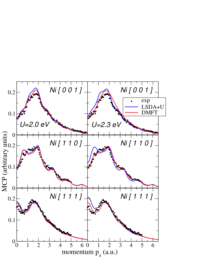
Figure 1: (color on-line) Compton profiles of Ni along the principal directions $[001]$, $[110]$ and $[111]$. Left column compares the LSDA+U/DMFT for $U=2.0$ eV with the results for $U=2.3$ eV. For both calculations $J=0.9$ eV and $T=400$ K have been used. The computed profiles LSDA (black-dotted), LSDA+U (blue-dashed) and LSDA+DMFT (red dashed-dot) are plotted in comparison to the experimental spectra (black-dotted). The calculated MCP profiles were convoluted with the experimental resolution 0.2 a.u.. Data were taken from Dixon et. al. [24].

The results of computations for the average Coulomb parameter $U=2.0$ eV are shown on the left column of Fig. 1. Along the [001] direction and around $p_{z}=0$ a.u. all LSDA(+U/DMFT) results seem to get close to the experimental data. Most significant differences are in the momentum range of $1$ a.u.$<p_{z}<2$ a.u., where also the maximum of the profile is located. Along the $[110]$ direction, both LSDA+U and LSDA+DMFT give similar results, overestimating the first maximum at around $0.5$ eV, show a minimum at around $1$ eV, instead of a maximum seen in the experiment and underestimate the experimental results in several regions above $2$ a.u. Along the $[111]$ direction, the maximum at $p_{z}=0$ a.u. is overestimated by all computations: the slight improvement of DMFT is not really significant, LSDA+U get very close to the maximum at around $2$ a.u. Overall dynamic correlations do really not improve significantly the agreement with the experimental data, as already at the level of LSDA reasonable good results has been obtained.

For a slightly larger value of $U=2.3$ eV the LSDA+U results start to depart more from the experimental data, while on contrary the DMFT results improve the agreement significantly. Along the $[001]$ in the entire low momentum region $p_{z}<2$ a.u. LSDA+U overestimates the spectrum, however for larger values of the momentum it captures the profile quite well. On the other hand, DMFT improves the momentum dependence below $p_{z}<2$ a.u., however it overestimates for values of the momentum in the range of 2 a.u. to 4 a.u. The largest difference between the “+U” and “+DMFT” corrections are seen along the [110] direction. This direction correspond to the shortest bond in the fcc structure. Here DMFT captures the peaks at around $0.5$ a.u. and the main peak at $2$ a.u., and continues very closely to the experimental data in the complete range of the computed momenta. LSDA+U captures only the main maximum and as a matter of fact produce worse results than LSDA. Along the $[111]$ direction DMFT get closer to the maximum at $p_{z}=0$ a.u. than LSDA+U. For $p_{z}>0$ a.u., the dip at $0.5$ a.u. is captured better within DMFT, while for higher momenta both the LSDA+U and LSDA+DMFT approaches follow essentially the same behavior.

Although both static and dynamic corrections to the MCP spectra are rather similar, we observe a clear tendency of LSDA+U to overestimate the experimental data while LSDA+DMFT correct some discrepancies. The following subsection presents the results for the difference in total Compton profiles with respect to the LSDA results, where distinctions because of static and dynamic corrections became more apparent.

II.2 Directional differences of Compton profiles

Fig. 2 shows the total Compton profiles differences computed according to Eq. (1) along the $[001]$ direction. The upper/lower part represents the DMFT/LSDA+U spectra after subtraction of LSDA results.

Figure 2: (color on-line) Computed difference Compton profiles of Ni along the $[001]$ direction for different values of $U$. The difference spectra of LSDA+DMFT with respect to LSDA, $U=2.0$ eV (black-dashed), $U=2.3$ eV (red-solid).

One can easily recognize common features in comparing the LSDA+U with LSDA+DMFT spectra. The Brillouin zone boundary along the [001] direction is represented by the $X(1/2,0,1/2)$-high symmetry point. The zone boundary is marked with the first dashed line and corresponds to the value of $k_{F}$ = 0.95 $a.u.$. The second dashed line is situated at $2k_{F}$ and is plotted to facilitate the comparison between the spectra. As one can see the LSDA+U spectra is sharper, since the DMFT self-energy contributes in smoothing out the spectra, however the peaks remain in the same positions. No additional broadening of the spectra has been applied. As a consequence of dynamic correlations within the first Brillouin zone, the $\Delta J_{[001]}$ has positive weight, on contrary to the LSDA+U results. We observe the Umklapp features identified in the MCP spectra of Ni [001] in several studies (at $\sim$ 1.2, 1.7, 2.7 and 3.7 a.u.) [24, 46, 47, 45] appearing in the $\Delta J_{[001]}$ as sharp deeps. For the region with $1.9<p_{z}<3.8$ a.u. (third and fourth Brillouin zone), electronic correlations produces negative difference weights. Similar observation can be made for the different values of $U$.

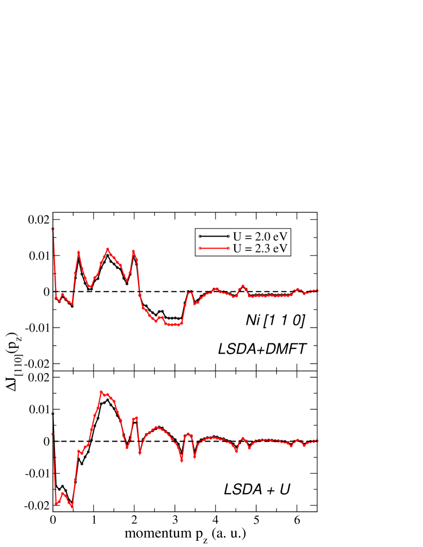
Figure 3: (color on-line) Computed difference Compton profiles of Ni along the [110] direction for different values of $U$. The difference spectra of LSDA+DMFT with respect to LSDA, $U=2.0~{}eV$ (black-dashed), $U=2.3~{}eV$ (red-solid).

Along the $[110]$ direction the Brillouin zone is intercepted at the $K$-point with the coordinate $3\pi/2a(1,1,0)$ in the Cartesian representation. Similarly to the $[001]$ direction, the position of the main peaks of the spectra are the same in the LSDA+U/DMFT calculations. The Umklapp features identified in the MCP spectra by several studies at $\sim 2.0$, $3.3$ and $4.6$ a.u. [24, 46, 47, 45] correspond to sharper peaks in the $\Delta J_{[110]}$ spectra. Again in LSDA+DMFT the spectra have an overall positive weight, due to correlation induced life time effects determined by the imaginary part of the self-energy. Also, Umklapp features are more visible in LSDA+U as no additional broadening is present.

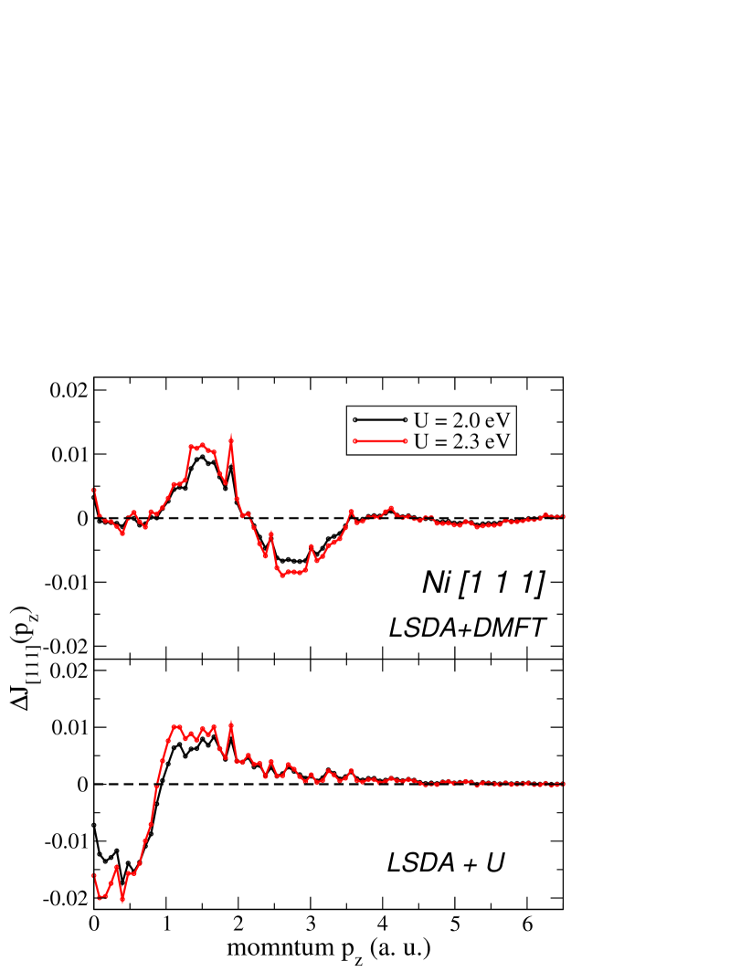
Figure 4: (color on-line) Computed difference Compton profiles of Ni along the $[111]$ direction for different values of $U$. The difference spectra of LSDA+DMFT with respect to LSDA, $U=2.0$ eV (black-dashed), $U=2.3$ eV (red-solid).

The same analysis can be performed upon the spectra in the $[111]$ direction. For momenta $p_{z}<k_{F}$ within the first Brillouin zone, $\Delta J_{[111]}$ computed with DMFT/+U have a negative contribution, whilst for the second and third zone the LSDA+DMFT difference spectra have weights with alternating sign. The $\Delta J_{[111]}$ spectra are essentially negative only within the first zone and from $p_{z}>1a.u.$ the LSDA+U spectra is positive.

The general tendency in both LSDA+U and LSDA+DMFT is that for larger $U$, maxima and minima are slightly stretched out, while the modulations remain the same. This is expected as the modulation of the Compton profile is connected to the topology of the Fermi surface. As was previously demonstrated, cuts of the momentum density remain unchanged with inclusion of correlation effects [48]. The overall change in the shape of the Compton spectra comparing DMFT versus LSDA/LSDA+U reflects the presence of the imaginary part of the dynamic local self-energy.

The comparison between the Compton spectra taken for different U values, along the same direction K allows to discuss the strength of local-correlation effects. In the same time comparing spectra obtained for a fixed $U$ value along different K, K^′ directions may reveal possible non-local-correlations effects. Although DMFT supplement the DFT-LDA part by a complex local and dynamic self-energy $\Sigma(z)$, the charge self-consistency of LDA+DMFT achieves indirect non-local effects. In the next subsection we analyze the differences between pairs of directional profiles also known as Compton profile anisotropies.

II.3 Compton profiles anisotropy and non-locality

Comparison between theoretical and experimental amplitudes of the Compton profile anisotropies for Ni have already been performed [49, 50, 51]. The computed anisotropy profiles $J_{[110]}-J_{[001]}$ and $J_{[111]}-J_{[001]}$ are shown in Fig. 5 that, in contrast with earlier work, reveal the role of correlations effects. In the upper panel the LSDA results are presented, while in the middle and lower panel the spectra obtained using LSDA+U and DMFT are seen. A very similar behavior, independent of the various level of sophistication to include the Coulomb interaction is visible.

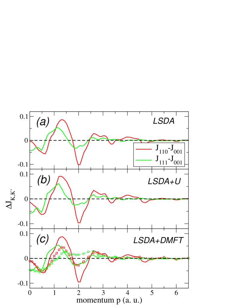
Figure 5: (color on-line) Theoretical Compton profile anisotropies of Ni. Upper panel (a) the anisotropy computed within LSDA. Lower pannels (b) and (c) show the LSDA+U and LSDA+DMFT results for $U=2.3$ eV, $J=0.9$ eV and $T=400$ K. Comparison with the experimental anisotropy is presented in pannel (c).

In the lower panel (c) we compare the anisotropy spectra with the corresponding experimental data of Anastassopoulos et. al. [51]. There is a rather satisfying agreement between the theory and experiment, in particular for the difference $J_{[110]}-J_{[001]}$ (Fig. 5 red lines) where the theoretical calculation follow most of the maxima and minima seen in the experiment. Here again no broadening has been used for the computed data. On the other hand for $J_{[111]}-J_{[001]}$ (Fig. 5 green lines) differences may be seen not only in the amplitude of the oscillation but also in the position of the minima/maxima. In Fig. 6 we show the comparison on a reduced momentum regime $0<p_{z}<1$ a.u. In the upper pannel of Fig. 6(a), the LSDA results are seen to overestimate in the range $0<p_{z}<0.2$ a.u. the experimental spectra plotted with dased lines. In the same momentum range the LSDA+U results underestimate the experimental data as seen in Fig. 6(b). Figure 6(c) shows the LSDA+DMFT results and one can see that the dynamic correlations capture at best the behaviour of anisotropy of the Compton profile in the region around the zero momentum $p_{z}<0.2$ a.u.

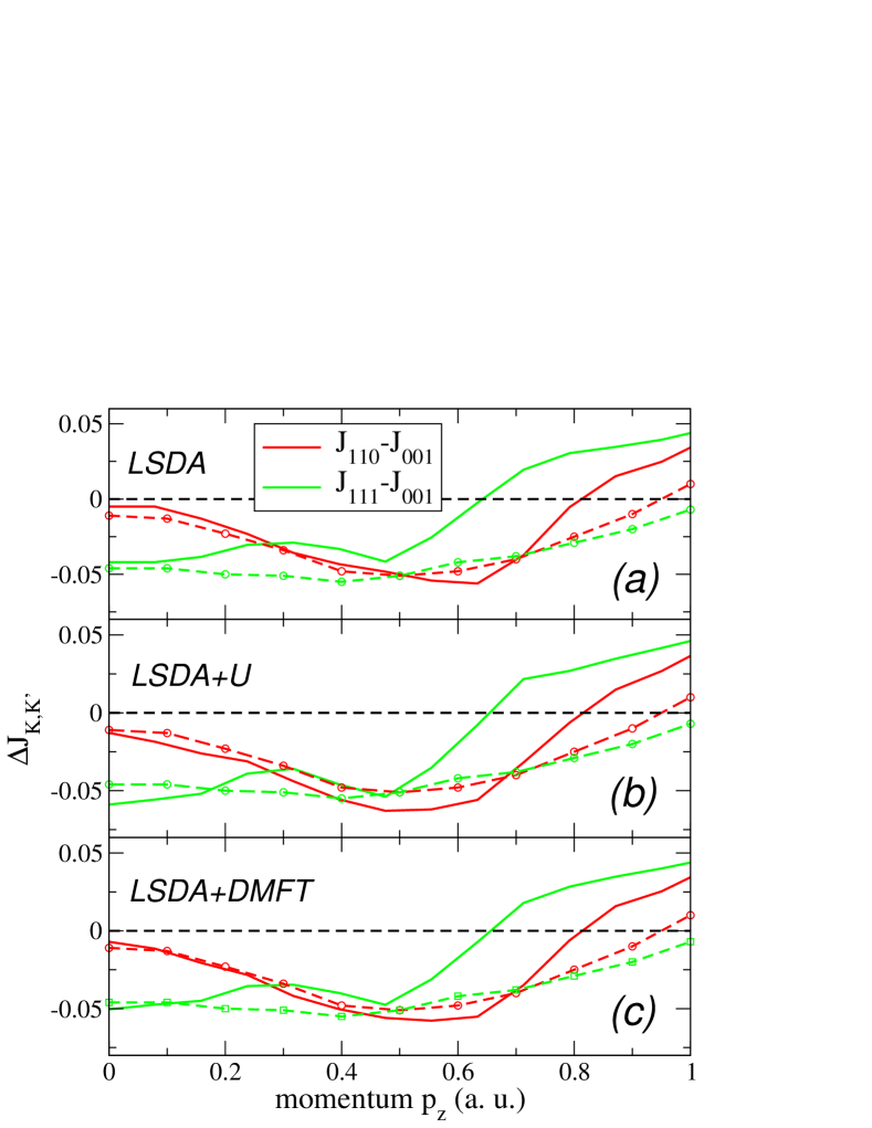
Figure 6: (color on-line) Theoretical Compton profile anisotropies of Ni in comparison with the experimental measurements. LSDA/LSDA+U results, panel (a)/(b) over/under-estimate the anisotropy data. DMFT results are in a good agreement with the experimental spectra in the range $0<p_{z}<0.2$ a.u. LSDA+U and LSDA+DMFT parameters are $U=2.3$ eV, $J=0.9$ eV and $T=400$ K.

Previous analysis attributed the discrepancies to the non-local correlation effects [52, 51], although no quantitative evidence has been presented. One possible alternative explanation for the results seen in Fig. 6 is that the density functional exchange-correlation potentials misplace the position of $d$-bands(orbitals). This agrees with the observation that LSDA overestimate the exchange splitting. Including static corrections using LSDA+U the exchange splitting is enhanced and therefore this does not correct upon the position of the $d$-bands, and equally does not improve on the anisotropy spectra. On the contrary, LSDA+DMFT is known to improve on the exchange splitting as a consequence of a Fermi-liquid type of self-energy and we equally see in the pannel of Fig. 6(c) although in a narrow momentum region $0<p_{z}<0.2$ a.u., an excellent agreement with the experimental anisotropies. As anisotropies in the Compton profile measures differences $J_{\bf K}-J_{\bf K^{\prime}}$ they indicate non-local effects, therefore Fig. 6(c) shows that local dynamic correlations may capture non-locality in a very narrow region around zero momentum as a consequence of full change self-consitency of LSDA+DMFT. In addition our results show that a description of the non-local-correlation effects is needed for a fruther improvement on the amplitudes of Compton profiles anisotropies for larger momenta.

III Kinetic energy corrections from relativistic and electronic correlations

The relativistic generalization of the Schrödinger theory of quantum mechanics to describe particles with spin 1/2 was achieved using the Dirac equation (see for example [53]). The construction of Dirac equation uses symmetry arguments and energy considerations, and it starts from the general Hamiltonian:

$$H=\frac{c}{i}{\bf\alpha}\cdot{\bf\nabla}+\frac{1}{2}\left(\beta-I\right)+V({\bf r}),$$ (3)

where ${\bf\alpha}$ and $\beta$ are standard Dirac matrices and $V({\bf r})$ represents a one particle effective potential. In the spirit of the non-relativistic DFT the effective potential consists of the Hartree term, an exchange correlation and a spin dependent part [54, 55]: $V({\bf r})=V_{H}({\bf r})+V_{xc}({\bf r})+\beta\sigma_{z}B({\bf r})$. Rigorous four-component relativistic many-electron calculations are hardly tractable in the spirit of four-component Dirac relativistic quantum mechanics [56]. It is important to note that many applications consider relativistic effects at one-component level, which is frequently called the scalar relativistic approach [57] which usually assume that corrections of higher order than $1/c^{2}$ can be neglected for chemical accuracy. Furthermore it is assumed that the effect of the spin-orbit coupling on the form of the orbitals may be neglected, allowing a partition of the Hamiltonian into a spin-independent and a spin-dependent part. The latter part is then only used in the final stage of the calculation to couple to the correlated many-electron problem. The analysis of components of the spin-orbit coupling was performed decoupling the longitudinal and transversal contributions  [54], allowing to identify the source of the most important spin-orbit induced phenomena in solids.

There are a few methods available to quantitatively assess the interplay between correlation and relativistic effects. Within the framework of DFT the recently developed LSDA+DMFT scheme demonstrates a clear potential in this direction. LSDA+DMFT has been systematically applied to $d$-, $f$-electron systems with various DMFT solvers [58]. From a pragmatic point of view perturbative solvers of DMFT written in adapted basis sets to include spin-orbit effects [38] are efficient tools for realistic multi atom/orbital calculations. This means that we in fact capture the interplay between relativistic and correlation effects at a more economical level of the theory: from the correlations point of view a perturbative solver is considered, while for the relativistic part the four-component was replaced by a two component formulation. For a single-particle in an effective potential $V_{eff}$, the most common transformation of the Dirac Hamiltonian (Eq. (3)) into the two component formulation: $H_{2comp}=UH_{4comp}U^{\dagger}$ is expressed as a unitary transformation [57], followed by a Taylor expansion in the fine structure constant $\propto 1/c^{2}$ and produce the following terms:

$$H^{BP} = (mc^{2}+V_{eff}+\frac{p^{2}}{2m})-\frac{p^{4}}{8m^{3}c^{2}}$$

$$- \frac{1}{8m^{2}c^{2}}(p^{2}V_{eff})+\frac{\hbar}{4m^{2}c^{2}}{\bf\sigma}(\nabla V_{eff}\times\vec{p})+...$$

The first terms in parenthesis in Eq. (III) represent the usual non-relativistic Hamiltonian, then the second one is the so called mass-velocity term, the third is called the Darwin term and the fourth operator describes the spin-orbit coupling (interaction). It can be analytically proved that the scalar mass-velocity and Darwin terms are unbounded from below. The resulting Breit-Pauli Hamiltonian ($H^{BP}$) also known as the first order relativistic Hamiltonian contain terms that are highly-singular and variationally instable. Therefore this operator is suitable to be used in the low order perturbation theory.

III.1 Moments of the differences of the Compton profiles

The measured Compton profile, or the momentum distribution enable in principle to obtain averages $\langle p^{n}\rangle$ directly from the experiment. On the computational side, the momentum space formulation allows to obtain the Compton profiles within the LSDA [59] and LSDA+DMFT [32, 33] for many systems. Further on additional information can be gained by taking moments of the difference between the correlated and non-correlated Compton profiles along different K-directions: $p_{z}||{\bf K}$

$$\langle p^{n}\rangle_{\bf K}=\int_{0}^{\infty}p_{z}^{n}\left[J^{+U/DMFT}_{\bf K}(p_{z})-J^{LSDA}_{\bf K}(p_{z})\right]dp_{z};$$

Recently we have computed the second moments $\langle p^{2}\rangle$  [33] along specific directions in Fe and Ni and discussed the effect of electronic correlations upon the kinetic energy per bonds. Aside from the kinetic energy $\langle p^{2}\rangle$, it is possible to obtain also relativistic energy corrections in the form of $\langle p^{4}\rangle$. In the present work we are interested to estimate the relativistic corrections to the kinetic energy that arises from the variation of electron mass with velocity, and how it may vary as a function of the local Coulomb interaction.

The second and the forth moments of the difference in the total Compton profiles, along the bond directions would provide some specific terms from the expansion (III). Namely we are going to evaluate the so called free particle relativistic kinetic energy ($H_{0}$) in terms of the second moments and its relativistic correction as the forth moment, along the bond directions of Ni. In order to compare the magnitude of second and fourth order moments one has to introduce a dimensionless quantity $p_{r}=p/mc$. In this reduced variable $H_{0}=mc^{2}\left((1/2)p_{r}^{2}-(1/8)p_{r}^{4}+...\right)$ and the relevant expectation values has the expression:

$$\langle H_{0}\rangle_{\bf K} = \int H_{0}\Delta J^{+U/DMFT}_{\bf K}(p_{z})dp_{z};(p_{z}||{\bf K})$$ (5)

$$\approx mc^{2}\left[\frac{1}{2}\langle p_{r}^{2}\rangle_{\bf K}-\frac{1}{8}\langle p_{r}^{4}\rangle_{\bf K}\right]$$

Table 1: Expectation values $\langle p_{r}^{n}\rangle$ along different direction computed within LSDA+U

		LSDA+U
$n$	$U$	[001]	[110]	[111]
	eV	10-6	10-6	10-6
2	2.0	1.06	2.65	6.37
	2.3	-2.12	0.53	5.84
4	2.0	-4.20 10-3	-1.18 10-3	4.26 10-3
	2.3	-6.29 10-3	-4.46 10-3	2.43 10-3

In the momentum space representation such integrals can be directly computed. We performed calculations for the second and fourth moments for different values of $U$ and different level of electronic correlations. The LSDA+U results are given in the Table 1. One can clearly see that the second and fourth order moments differ significantly along different directions. For $U=2$ eV all second moments are positive for all directions, while for larger $U=2.3$ eV along [001] the second moment is negative. In the reduced representation $p/mc$ the magnitude of these moments is of order $10^{-6}$. The forth order moments are 3 order of magnitude smaller than the second order moments, and are negative along the [001] and [110] directions. Along the [111] direction the forth order moment remain positive for all $U$ values. Note that moments decrease in magnitude as the distance is increasing: the largest moments are obtained for the nearest neighbors distances, which are the shortest bonds. For Ni, this corresponds to the [110] direction. Directional averaging over all second order moments provides the kinetic energy, while a similar average over the 4-th order moments provides the relativistic corrections to the kinetic energy.

The moments computed in LSDA+DMFT are given in Table 2. On contrary to the LSDA+U, using DMFT produces a Compton profile having negative second moments along all directions and for all studied values of $U=2$ eV and $2.3$ eV.

Table 2: Expectation values $\langle p_{r}^{n}\rangle$ along different direction computed within LSDA+DMFT

		LSDA+DMFT
$n$	$U$	[001]	[110]	[111]
	eV	10-6	10-6	10-6
2	2.0	-7.43	-6.90	-4.78
	2.3	-11.15	-8.50	-6.37
4	2.0	8.75 10-3	-5.92 10-3	-3.69 10-3
	2.3	-1.12 10-3	-7.62 10-3	-6.38 10-3

Note the qualitative difference between the LSDA+U and LSDA+DMFT second moments: while the former mean field (LSDA+U) approach produce second moments with different signs depending on the directions, within the later dynamic (LSDA+DMFT) approach correction is always negative. Similarly to our previous results [33] we see that the positive difference at low momentum region $0<p_{z}<2$ a.u. is completely overruled by the negative weights at higher momenta, which leads to the overall negative values for the correction obtained in DMFT. In LSDA+U a negative second moment is obtained along [001] and positive for the other two directions. The positive second moment is obtained as the Compton profile computed in the mean field (LSDA+U) approach always is larger than the corresponding LSDA profile, for any value of the moment $p_{z}$. In order to discuss correction to the kinetic energies, we computed the weighted sum of the nearest neighbors, i.e. six times the contribution along [001], 12 times the contribution along [110] and 8 times the contribution along [111] divided by the total number of neighbors (26). Fig. 7 summarizes the computed results. The inset shows the directional average of the second moment which is positive in LSDA+U and negative in DMFT, whilst the corrections to the kinetic energy is negative in both +U/DMFT calculations.

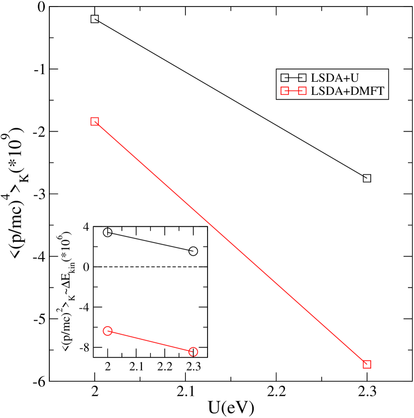
Figure 7: (color on-line) Averaged forth (second, in inset) order moments of the difference Compton profiles computed within DMFT (red solid) and LSDA+U (black dashed), along different directions and for the Coulomb parameters $U=2$ eV$/2.3$ eV, $J=0.9$ eV and $T=400$ K.

IV Discussions and Conclusion

The influence of electronic correlations on the Compton profiles of Ni has been discussed within the framework of DFT comparing the results of mean field LSDA+U and beyond mean-field LSDA+DMFT. According to our results, the mean field decoupling of the interaction (+U) overestimates slightly the MCP spectra, while dynamic correlations improve the agreement with experiment. To reveal differences between the LSDA+U and LSDA+DMFT approaches we studied the directional differences, i.e. differences of Compton profiles with respect to the LSDA spectra. Overall the difference spectra follow a similar momentum dependence with visible deviations in the low momentum region. A qualitative difference is evidenced in this region: within the mean field approach (+U) negative differences are seen while in the dynamic case, the opposite result is obtained. In other words, the mean field LSDA+U Compton spectra have a smaller weight in the low energy region than the corresponding LSDA+DMFT Compton spectra. According to our recent picture of momentum redistribution because of interaction [33] we conclude that the weight from low momentum distribution is shifted towards the higher momentum region in the LSDA+U spectra. This is in agreement with the naive picture of the effects of LSDA+U on the spectral weight distribution shifting weights towards higher energies. In the Compton scattering language, photons would scatter accordingly on moving electrons situated in higher energy bands, although this does not mean that the electrons are moving faster, explaining the fact that there are no dramatic changes in the Compton spectra (differences of order of $\pm 0.02$) shown in Figs. 2, 3 and 4. On the contrary to the LSDA+U results, in the DMFT calculations the Fermi liquid type of self-energy determines the spectral weight transfer towards the low energy region, and accordingly the spectra of photons scattering on the renormalized electronic structure would be redistributed towards low momenta. Similar conclusions have been reached in our previous studies [32, 33].

In the analysis of the Compton profile anisotropies we found that the LSDA+DMFT results describe well the momentum region of $0<p_{z}<0.2$ a.u. which is a consequence of the presence of a local and dynamic self-energy that properly locates the position of Ni $d$-bands, as seen in various calculations. The limited momentum range is due to the inherent DMFT approximation that the self-energy neglect spatial fluctuations.

In order to assess the capability of electronic correlations to influence the kinetic energy along specific directions we have computed the second and the fourth order moments of the Compton spectra considering the reduced momentum $p_{r}=p/mc$. Although the fourth order moments are significantly smaller, $\langle p_{r}^{4}\rangle\propto 10^{-3}\langle p_{r}^{2}\rangle$, an overall non-negligible contribution is obtained (see Eq.(5)). Within LSDA+U the second moment has a positive sign, which is in agreement with the description of the momentum redistribution towards higher momenta descried above, except for the [001] direction. The overall energy correction is still positive in LSDA+U as seen in the inset of Fig. 7. Negative second moments are obtained along all directions in DMFT and produce a negative kinetic energy contribution. The relativistic corrections to the kinetic energy are both negative and we see that dynamic correlations (LSDA+DMFT) generate larger relativistic corrections to the one-particle kinetic energy in comparison to their mean field (LSDA+U) counter part.

As an overall conclusion in the range of the studied values of $U$ qualitative and quantitative differences are seen in the Compton profiles depending weather the LSDA is supplemented with static or dynamic many-body effects. An important message is that relativistic effects and electronic correlations may have a non-trivial interplay and dynamic correlations determine larger relativistic corrections in the electronic structure of solids. Further investigations are necessary for a quantitative assessments of such effects.

V acknowledgments

Financial support of the Deutsche Forschungsgemeinschaft through FOR 1346, the DAAD and the CNCS - UEFISCDI (project number PN-II-ID-PCE-2012-4-0470) is gratefully acknowledged. JM acknowledge also the CENTEM project, reg. no. CZ.1.05/2.1.00/03.0088, co-funded by the ERDF as part of the Ministry of Education, Youth and Sports OP RDI programme.

References

- Aubert and Michelutti [1977] G. Aubert and B. Michelutti, Physica B 86-88, 295 (1977).
- Yang et al. [2001] I. Yang, S. Y. Savrasov, and G. Kotliar, Phys. Rev. Letters 87, 216405 (2001).
- Gersdorf [1978] R. Gersdorf, Phys. Rev. Letters 40, 344 (1978).
- Bünemann et al. [2008] J. Bünemann, F. Gebhard, T. Ohm, S. Weiser, and W. Weber, Phys. Rev. Letters 101, 236404 (2008).
- Leung et al. [1991] T. C. Leung, C. T. Chan, and B. N. Harmon, Phys. Rev. B 44, 2923 (1991).
- Eastman et al. [1978] D. E. Eastman, F. J. Himpsel, and J. A. Knapp, Phys. Rev. Lett. 40, 1514 (1978).
- Dietz et al. [1978] E. Dietz, U. Gerhardt, and C. J. Maetz, Phys. Rev. Lett. 40, 892 (1978).
- Himpsel et al. [1979] F. J. Himpsel, J. A. Knapp, and D. E. Eastman, Phys. Rev. B 19, 2919 (1979).
- Eastman et al. [1980] D. E. Eastman, F. J. Himpsel, and J. A. Knapp, Phys. Rev. Lett. 44, 95 (1980).
- Eberhardt and Plummer [1980] W. Eberhardt and E. W. Plummer, Phys. Rev. B 21, 3245 (1980).
- Guillot et al. [1977] C. Guillot, Y. Bally, J. Paigné, J. Lecante, K. P. Jain, P. Thiry, R. Pinchaux, Y. Petroff, and L. M. Falicov, Phys. Rev. Letters 39, 1632 (1977).
- Metzner and Vollhardt [1989] W. Metzner and D. Vollhardt, Phys. Rev. Letters 62, 324 (1989).
- Georges et al. [1996] A. Georges, G. Kotliar, W. Krauth, and M. J. Rozenberg, Rev. Mod. Phys. 68, 13 (1996).
- Kotliar and Vollhardt [2004] G. Kotliar and D. Vollhardt, Phys. Today 57, 53 (2004).
- Lichtenstein et al. [2001] A. I. Lichtenstein, M. I. Katsnelson, and G. Kotliar, Phys. Rev. Letters 87, 067205 (2001).
- Chioncel et al. [2003] L. Chioncel, L. Vitos, I. A. Abrikosov, J. Kollár, M. I. Katsnelson, and A. I. Lichtenstein, Phys. Rev. B 67, 235106 (2003).
- Minár et al. [2005] J. Minár, L. Chioncel, A. Perlov, H. Ebert, M. I. Katsnelson, and A. I. Lichtenstein, Phys. Rev. B 72, 045125 (2005).
- Braun et al. [2006] J. Braun, J. Minár, H. Ebert, M. I. Katsnelson, and A. I. Lichtenstein, Phys. Rev. Lett. 97, 227601 (2006).
- Grechnev et al. [2007] A. Grechnev, I. D. Marco, M. I. Katsnelson, A. I. Lichtenstein, J. Wills, and O. Eriksson, Phys. Rev. B 76, 035107 (2007).
- Sánchez-Barriga et al. [2009] J. Sánchez-Barriga, J. Fink, V. Boni, I. Di Marco, J. Braun, J. Minár, A. Varykhalov, O. Rader, V. Bellini, F. Manghi, et al., Phys. Rev. Lett. 103, 267203 (2009).
- Granas et al. [2012] O. Granas, I. di Marco, P. Thunström, L. Nordström, O. Eriksson, T. Björkman, and J. Wills, Comp. Mat. Sci. 55, 295 (2012).
- Sánchez-Barriga et al. [2012] J. Sánchez-Barriga, J. Braun, J. Minár, I. Di Marco, A. Varykhalov, O. Rader, V. Boni, V. Bellini, F. Manghi, H. Ebert, et al., Phys. Rev. B 85, 205109 (2012).
- Kubo and Asano [1990] Y. Kubo and S. Asano, Phys. Rev. B 42, 4431 (1990).
- Dixon et al. [1998] M. A. G. Dixon, J. A. Duffy, S. Gardelis, J. E. McCarthy, M. J. Cooper, S. B. Dugdale, T. Jarlborg, and D. N. Timms, J. Phys.: Condensed Matter 10, 2759 (1998).
- Timms et al. [1990] D. N. Timms, A. Brahmia, M. J. Cooper, S. P. Collins, S. Hamouda, D. Laundy, C. Kilbourne, and M.-C. S. Larger, J. Phys.: Condensed Matter 2, 3427 (1990).
- Eisenberger et al. [1972] P. Eisenberger, L. Lam, P. M. Platzman, and P. Schmidt, Phys. Rev. B 6, 3671 (1972).
- Lundqvist and Lydén [1971] B. I. Lundqvist and C. Lydén, Phys. Rev. B 4, 3360 (1971).
- Bauer and Schneider [1983] G. E. W. Bauer and J. R. Schneider, Z. Physik B 54, 17 (1983).
- Bauer [1984] G. E. W. Bauer, Phys. Rev. B 30, 1010 (1984).
- Bauer and Schneider [1984] G. E. W. Bauer and J. R. Schneider, Phys. Rev. Lett. 52, 2061 (1984).
- Bauer and Schneider [1985] G. E. W. Bauer and J. R. Schneider, Phys. Rev. B 31, 681 (1985).
- Benea et al. [2012] D. Benea, J. Minár, L. Chioncel, S. Mankovsky, and H. Ebert, Phys. Rev. B 85, 085109 (2012).
- Chioncel et al. [2014] L. Chioncel, D. Benea, H. Ebert, I. Di Marco, and J. Minár, Phys. Rev. B 85, 085109 (2014).
- Ebert et al. [2011] H. Ebert, D. Ködderitzsch, and J. Minár, Rep. Prog. Phys. 74, 096501 (2011).
- Vosko et al. [1980] S. H. Vosko, L. Wilk, and M. Nusair, Can. J. Phys. 58, 1200 (1980).
- Monkhorst and Pack [1976] H. J. Monkhorst and J. D. Pack, Phys. Rev. B 13, 5188 (1976).
- Katsnelson and Lichtenstein [2002] M. I. Katsnelson and A. I. Lichtenstein, Eur. Phys. J. B (2002).
- Pourovskii et al. [2005] L. V. Pourovskii, M. I. Katsnelson, and A. I. Lichtenstein, Phys. Rev. B (2005).
- Marco et al. [2009] I. D. Marco, J. Minár, S. Chadov, M. I. Katsnelson, H. Ebert, and A. I. Lichtenstein, Phys. Rev. B 79, 115111 (2009).
- Minár [2011] J. Minár, J. Phys.: Condensed Matter 23, 253201 (2011).
- Aryasetiawan et al. [2004] F. Aryasetiawan, M. Imada, A. Georges, G. Kotliar, S. Biermann, and A. I. Lichtenstein, Phys. Rev. B 70, 195104 (2004).
- Szotek et al. [1984] Z. Szotek, B. L. Gyorffy, G. M. Stocks, and W. M. Temmerman, J. Phys. F: Met. Phys. 14, 2571 (1984).
- Benea et al. [2006] D. Benea, S. Mankovsky, and H. Ebert, Phys. Rev. B 73, 094411 (2006).
- Benea [2004] D. Benea, Ph.D. thesis, LMU München (2004).
- Baruah et al. [2000] T. Baruah, R. R. Zope, and A. Kshirsagar, Phys. Rev. B 62, 16435 (2000).
- Kubo [2004] Y. Kubo, J. Phys. Chem. Solids 65, 2077 (2004).
- Kakutani et al. [2003] Y. Kakutani, Y. Kubo, A. Koizumi, N. Sakai, B. L. Ahuja, and B. K. Sarma, J. Phys. Soc. Japan 72, 599 (2003).
- Majundar [1965] C. K. Majundar, Phys. Rev. 140, A227 (1965).
- Eisenberger and Reed [1974] P. Eisenberger and W. A. Reed, Phys. Rev. B 9, 3242 (1974).
- Wang and Callaway [1975] C. S. Wang and J. Callaway, Phys. Rev. B 11, 2417 (1975).
- Anastassopoulos et al. [1990] D. L. Anastassopoulos, G. D. Priftis, N. I. Papanicolau, N. C. Bacalis, and D. A. Papaconstantopoulos, J. Phys.: Condensed Matter 3, 1099 (1990).
- Rollason et al. [1987] A. J. Rollason, J. R. Schneider, D. S. Laundy, R. S. Holt, and M. J. Cooper, J. Phys. F: Met. Phys. 17, 1105 (1987).
- Strange [1998] P. Strange, Relativistic Quantum Mechanics (Cambridge: University Press, 1998).
- Ebert et al. [1997] H. Ebert, H. Freyer, and M. Deng, Phys. Rev. B 56, 9454 (1997).
- Ebert [2000] H. Ebert, in Electronic Structure and Physical Properties of Solids, edited by H. Dreyssé (Springer, Berlin, 2000), vol. 535, p. 191.
- Dirac [1928] P. A. M. Dirac, Proc. Roy. Soc. (London) A 118, 351 (1928).
- Foldy and Wouthuysen [1950] L. L. Foldy and S. A. Wouthuysen, Phys. Rev. 78, 29 (1950).
- Kotliar et al. [2006] G. Kotliar, S. Y. Savrasov, K. Haule, V. S. Oudovenko, O. Parcollet, and C. A. Marianetti, Rev. Mod. Phys. 78, 865 (2006).
- Cooper [1985] M. J. Cooper, Rep. Prog. Phys. 48, 415 (1985).