Effects of complex parameters on classical trajectories of
Hamiltonian systems

Abstract

Anderson et al have shown that for complex energies, the classical trajectories of real quartic potentials are closed and periodic only on a discrete set of eigencurves. Moreover, recently it was revealed that, when time is complex $t$ $(t=t_{r}e^{i\theta_{\tau}}),$ certain real hermitian systems possess close periodic trajectories only for a discrete set of values of $\theta_{\tau}$. On the other hand it is generally true that even for real energies, classical trajectories of non $\mathcal{PT}$- symmetric Hamiltonians with complex parameters are mostly non-periodic and open. In this paper we show that for given real energy, the classical trajectories of complex quartic Hamiltonians $H=p^{2}+ax^{4}+bx^{k}$, (where $a$ is real, $b$ is complex and $k=1$ $or$ $2$) are closed and periodic only for a discrete set of parameter curves in the complex $b$-plane. It was further found that given complex parameter $b$, the classical trajectories are periodic for a discrete set of real energies (i.e. classical energy get discretized or quantized by imposing the condition that trajectories are periodic and closed). Moreover, we show that for real and positive energies (continuous), the classical trajectories of complex Hamiltonian $H=p^{2}+\mu x^{4},$ ($\mu=\mu_{r}e^{i\theta})$ are periodic when  $\theta=4tan^{-1}[(n/(2m+n))]$ for $\forall$ $n$ and $m\in\mathbb{Z}$.

I Introduction

In recent years, classical behavior of non-Hermitian Hamiltonian systemsR1 ; R2 ; R3 ; R4 ; R5 as well as classical motion of Hermitian systems for complex energiesR6 ; R7 ; R8 ; R9 ; R10 ; R11 ; R12 ; R13 ; R14 ; R15 ; R16 have attracted much interest. Investigation of classical mechanics in the complex domain is useful for understanding various classical and quantum mechanical phenomena such as barrier tunneling, dynamical tunnelingR17 ; R18 , classical and quantum chaosR7 ; R19 , quantum correspondence principle,complex forms of uncertainty relations and the semiclassical limit of complex quantum field theories.

Since the earlier work on classical motion of non-Hermitian systems R6 ; R7 , there have been several interesting results found on the various aspects of the subjectR8 ; R9 ; R10 ; R11 ; R12 ; R13 ; R14 ; R15 ; R16 . Numerical and analytical investigations have revealed that when energies are real, classical trajectories of complex $\mathcal{PT}$-symmetric non Hermitian systems are closed and periodic. However, when energies of these systems are complex, the periodic trajectories usually become non periodic and openR15 ; R19 . Recently it was shown that even though most of the trajectories corresponding to complex energies are open and non periodic, for some systems, there are special discrete sets of curves in the complex-energy plane for which the trajectories are periodicR20 . On the other hand, in non-Hermitian and non $\mathcal{PT}$-symmetric Hamiltonian systems, even for real energies, almost all trajectories except a few are non-periodic and open. It was also shown recently that when time is taken as a complex quantity with a specific fixed phase angle or as a specific complex function, non periodic trajectories of 1-D Hamiltonian systems become periodic and closedR21 .

In this paper we investigate the classical trajectories from a different point of view. Here we examine clasical behavior of the complex Hamiltonian $H=p^{2}+ax^{4}+bx^{k}$, (where $k=1$, $2$, and $a$ is real such that $H$ is not $\mathcal{PT}$-symmetric) for complex parameter $b$ and real energy $E$. Outline of the paper is as follows. In the section II, analytic expressions for complex trajectories are derived.Expressions for periods of the periodic trajectories as well as time taken by unbounded trajectories to escape to infinity are found in terms of $b$ and energy $E$.  We will show that for given real energy, the classical trajectories of the above quartic Hamiltonian are open except for a discrete set of parameter values in the complex $b$-plane. In section III we study how trajectories behave when energy is real and $b$ is a fixed complex parameter. The classical trajectories of complex Hamiltonian $H=p^{2}+\mu x^{4},$ ($\mu=re^{i\theta})$ is investigated for real energies in section IV and concluding remarks are given in section V.

II Classical trajectories of $H=p^{2}+ax^{4}+bx^{k}$

In this section first we study in detail the classical motion of the complex quartic anharmonic oscillator. We assume that the Hamiltonian has the form

$$H=p^{2}+ax^{4}+bx^{k}$$ (1)

where $a$ is a real positive constant, $b$ is a complex constant and $k=1$ or $2$. First we derive expressions for $x(t)$ and the period for the above Hamiltonian. When it is needed, value of $k$ is chosen as $1$ or $2$. Throughout this paper mass of the particle is taken as half $(i.e.2m=1).$ The equation of motion is

$$\frac{dx}{dt}=p=2\sqrt{E-ax^{4}-bx^{k}}$$ (2)

The turning points of this system are taken as $x_{0},x_{1},x_{2}$ and $x_{3}$ and by integrating equation(2)we have

$$\int\frac{dx}{\sqrt{\left(x-x_{0}\right)(x-x_{1})(x-x_{2})(x-x_{3})}}=2\sqrt{a}e^{i\pi/2}t+c$$ (3)

where $c$ is the constant of integration which depends on initial conditions. The left-hand side of the above equation is an elliptic integral of the first kind and hence equation (3) becomes

$$\frac{2}{\sqrt{\left(x_{0}-x_{2}\right)\left(x_{1}-x_{3}\right)}}{\small F}\left(\sin^{-1}\left[\sqrt{\frac{\left(x-x_{1}\right)(x_{0}-x_{2})}{\left(x-x_{0}\right)(x_{1}-x_{2})}}\right],\frac{\left(x_{1}-x_{2}\right)(x_{0}-x_{3})}{\left(x_{0}-x_{2}\right)(x_{1}-x_{3})}\right)$$

$$=2\sqrt{a}e^{i\pi/2}t+c$$ (4)

where $F$ is an elliptic function. We invert the above equation in terms of Jacobian elliptic function ‘$sn$’ as

$$x\left(t\right)=\frac{x_{1}\left(x_{0}-x_{2}\right)-x_{0}(x_{1}-x_{2})sn^{2}(u)}{\left(x_{0}-x_{2}\right)-(x_{1}-x_{2})sn^{2}(u)}$$ (5)

where $u=\sqrt{a\left(x_{0}-x_{2}\right)\left(x_{1}-x_{3}\right)}e^{i\pi/2}t+\alpha$ and modulus $\kappa=\left[\frac{\left(x_{1}-x_{2}\right)(x_{0}-x_{3})}{\left(x_{0}-x_{2}\right)(x_{1}-x_{3})}\right]^{1/2}$ and $\alpha$ is an arbitrary constant which is determined by the initial conditions. Note that $x(t)$ in the above equation is still a solution of (3), when $x_{0},x_{1},x_{2}$ and $x_{3}$ are cyclically changed (e.g. $x_{3}\rightarrow x_{0}\rightarrow x_{1}\rightarrow x_{2}\rightarrow x_{3}$). In order to understand how the trajectories behave, we need to recognize the periodic, bounded and unbounded properties of the function $x\left(t\right)$. First we find complementary modulus $\kappa^{\prime}$ and complete elliptic functions $K$ and $K^{\prime}$. They are defined by

$$\kappa^{{\prime}^{2}}=1-\kappa^{2}=\frac{\left(x_{0}-x_{1}\right)(x_{2}-x_{3})}{\left(x_{0}-x_{2}\right)(x_{1}-x_{3})}$$ (6)

$$K=\overset{\frac{\pi}{2}}{\underset{0}{\int}}(1-\kappa^{2}\sin^{2}\left(\phi\right))^{-\frac{1}{2}}d\phi$$ (7)

$$K^{\prime}=\overset{1}{\underset{0}{\int}}\left(1-t^{2}\right)^{-\frac{1}{2}}\left(1-\kappa^{{\prime}^{2}}t^{2}\right)^{-\frac{1}{2}}dt.$$ (8)

$K$ and $K^{\prime}$ are evaluated directly from the above equations and they are independent of phase angle $\theta$.

The trajectory $x(t)$ is given by $\ x\left(t\right)=\frac{x_{1}\left(x_{0}-x_{2}\right)-x_{0}(x_{1}-x_{2})sn^{2}(u)}{\left(x_{0}-x_{2}\right)-(x_{1}-x_{2})sn^{2}(u)}.$ The condition of trajectory become unbounded and the particle escapes to infinity is

$$\left(x_{0}-x_{2}\right)-(x_{1}-x_{2})sn^{2}(u)=0\vskip 12.0pt plus 4.0pt minus 4.0pt$$ (9)

where $u=\sqrt{a\left(x_{0}-x_{2}\right)\left(x_{1}-x_{3}\right)}e^{i\pi/2}t+\alpha$ satisfied for some real positive $t$ and the time taken for the particle to escape to $\infty$ is give by

$$T_{\infty}=\frac{\left(sn^{-1}(z_{0})-\alpha\right){\small e}^{-i\pi/2}}{\sqrt{a\left(x_{0}-x_{2}\right)\left(x_{1}-x_{3}\right)}}$$ (10)

where $z_{0}=\sqrt{\frac{(x_{0}-x_{2})}{(x_{1}-x_{2})}}.$ ‘$sn$’ is doubly periodic with period $4mK+2niK^{\prime}$ where $m$ and $n$ are integers. Therefore the condition for the trajectory to become periodic and particle does not escape to infinity is

$$\sqrt{a\left(x_{0}-x_{2}\right)\left(x_{1}-x_{3}\right)}e^{i\pi/2}t=4mK+2niK^{\prime}\ ;\ \ \ \ m,\ n\ \epsilon\ \mathbb{Z}.$$ (11)

and $t<T_{\infty}.$ Then the trajectory is periodic with the period.

$$T_{p}=\frac{\left(4mK+2niK^{\prime}\right){\small e}^{-i\pi/2}}{\sqrt{a\left(x_{0}-x_{2}\right)\left(x_{1}-x_{3}\right)}}.$$ (12)

Note that if $T_{p}>T_{\infty}$ the trajectory is still nonperiodic. By imposing the condition that Im$\left(T_{p}\right)=0$, we have

$$r\equiv\frac{n}{m}=\frac{Im[2iK/z]}{Im\left[K^{\prime}/z\right]};\ \ \ \ m,\ n\ \epsilon\ \mathbb{Z}$$ (13)

where $z=\sqrt{a\left(x_{0}-x_{2}\right)\left(x_{1}-x_{3}\right)}.$ Since $n$ and $m$ are integers and the energy $E$ is fixed, $r$ is rational and the equation (13) provides a discrete set of parameter values in the complex $b$ plane for which classical trajectories are periodic. Let $b=b_{r}e^{i\theta}.$ Figures 1a and 1b show how the ratio $r$ varies with discrete values of $\theta$ for the cases $k=1$ and $k=2$ respectively. Without loss of generality, the energy $E$ is taken as unity as it is real. The results can be generalized for any real energy $E$ by simple rescaling of $x$ and $t$.

III Discretization of classical energy

Next we consider the case when parameter $b$ is a fixed complex number and $E$ is a variable (Assume $a=1$ and $b=1+i.$). As a result, the equation (13) allows only a discrete set of values of $E$ for which trajectories are periodic. It was found that these discrete values of $E$ can be either real or complex satisfying the condition (13). Table 1 and Table 2 show some real discrete values of $E$ which make trajectories periodic when $k=1$ and $k=2$ respectively. Figures 2 and 3 show the periodic trajectories of systems $k=1$ and $k=2$ for two values of real energies.

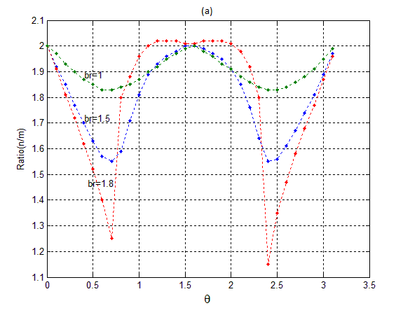
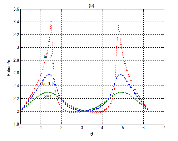
Figure 1: By applying the condition that classical trajectories are periodic, we obtain discrete values of $\theta$ for a fixed value of $b_{r}$. (a) shows how the ratio $r$  varies with complex phase angle $\theta$ of the potential $V(x)=x^{4}+b_{r}e^{i\theta}x\$. In order to have periodic trajectories, $r$ ($r\equiv\frac{n}{m}$) has to be rational and hence only discrete values of $\theta$ satisfy the condition (13). Each point in the graph represent such a value. (b) same as (a) but for the potential $V(x)=x^{4}+b_{r}e^{i\theta}x^{2}$

Moreover, it was found that if energy $E$ is corresponding to the periodic trajectories of $p^{2}+ax^{4}+bx$ then $-E$ will be the energy which makes trajectories of $p^{2}-ax^{4}+i\overline{b}x$ ( $\overline{b}$ is the complex conjugate of $b$) periodic. Further $E$ and $-E$ are solutions corresponding to the same $n$ and $m$ in the periodic condition (13) for these two Hamiltonians respectively. In other words if $S_{E}$ is the discrete set of energies for which classical trajectories of $p^{2}+ax^{4}+bx$ are periodic then $S_{-E}$ is the set of energies for which trajectories of $p^{2}-ax^{4}+i\overline{b}x$ are periodic. Figures 4a and 4b show two periodic trajectories illustrating the above claim.

m	n	E
1	1	0.27499
1	2	0.71624
1	3	0.78605
2	3	0.60480
2	5	0.74280
2	1	-0.28103
3	1	-0.53968
3	2	-0.07449
5	2	-0.42562

Table 1: Classical energy spectrum corresponding to periodic trajectories of $V(x)=x^{4}+(1+i)x$ for various $(m,n).$

m	n	E
1	1	-0.02143
1	2	-0.16951
1	3	-0.32417
2	3	-0.08940
2	5	-0.24827
2	1	1.45802
3	1	2.99725
3	2	0.81963
5	2	2.17849

Table 2: Classical energy spectrum corresponding to periodic trajectories of $V(x)=x^{4}+(1+i)x^{2}$ for various $(m,n)$

IV Periodic Classical trajectories of $H=p^{2}+\mu_{r}e^{i\theta}x^{4}$

Next we assume that $a=\mu$ and $b=0$ in the Hamiltonian (1). Then new Hamiltonian has the form

$$H=p^{2}+\mu x^{4}$$ (14)

where $\mu$ is complex and $\mu=\mu_{r}e^{i\theta}$. The equation of motion is

$$\frac{dx}{dt}=2\sqrt{E-\mu x^{4}}$$ (15)

where $E$ is the total energy. Following the same procedure as in section II, we obtain required equations. By integrating (15) we have

$$\int\frac{dx}{\sqrt{E-\mu x^{4}}}=2t+c$$ (16)

where $c$ is the constant of integration which depends on initial conditions. The left-hand side of the above equation is an elliptic integral of the first kind and hence equation (16) becomes

$${\small F}\left(\sin^{-1}\left[\left(\frac{\mu}{E}\right)^{1/4}x(t)\right],-1\right){\small=2}\left(\mu E\right)^{1/4}{\small t+\alpha}$$ (17)

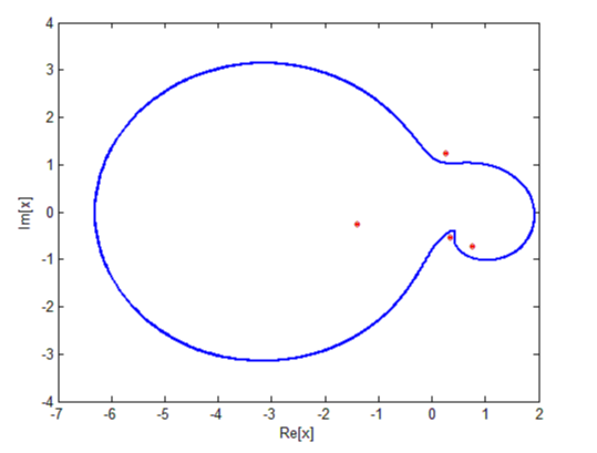
Figure 2: A periodic trajectory corresponding to $(m,n)=(1,2)$ for the quartic potential $V(x)=x^{4}+(1+i)x$ with real energy $E=0.71624$

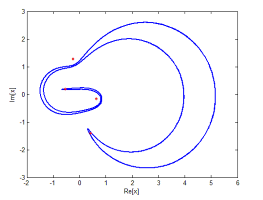
Figure 3: A periodic trajectory for the quartic potential $V(x)=x^{4}+(1+i)x^{2}$ corresponding to $(m,n)=(3,2)$ with real energy $E=0.81963$

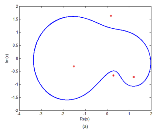
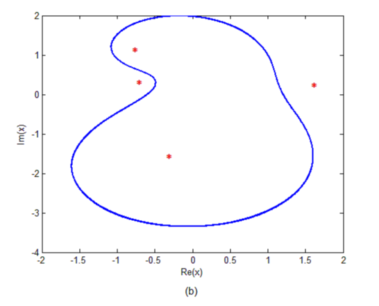
Figure 4: A typical periodic classical trajectories of the potentials (a) $V(x)=x^{4}+(2+3i)x$ and (b) $V(x)=-x^{4}+(3+2i)x$ . Energies of trajectories corresponding to figures (a) and (b) are $E=2.42227$ and $E=-2.42227$ respectively. The four turning points are marked as dots.

where $\alpha=\left(\mu E\right)^{1/4}c$ and $F$ is an elliptic function. We invert the above equation in terms of Jacobian elliptic function ‘$sn$’ as

$$x\left(t\right)=\left(\frac{E}{\mu}\right)^{1/4}sn\left(2\left(\mu E\right)^{1/4}t+\alpha\ ;\ -1\right).$$ (18)

Note that modulus $\kappa^{2}=-1$ for the above problem. $K$ and $K^{\prime}$ are defined in (7) and (8) and

$$\kappa^{\prime^{2}}=1-\kappa^{2}=2.$$ (19)

Then $K$ and $K^{\prime}$ are obtained as

$$K=\frac{\sqrt{\pi}\Gamma\left(1/4\right)}{4\Gamma\left(3/4\right)}$$ (20)

$$K^{\prime}=\frac{\sqrt{\pi}\Gamma\left(1/4\right)}{4\Gamma\left(3/4\right)}\left(1-i\right)$$ (21)

As in the previous sections the condition of trajectory become periodic and particle does not escape to infinity is

$$2\left(\mu E\right)^{1/4}t=4mK+2niK^{\prime}\ ;\ \ \ m,\ n\ \epsilon\ \mathbb{Z}.$$ (22)

Then the trajectory is periodic with the period

$$T_{p}(\mu_{r})=\frac{2mK+niK^{\prime}}{\left(\mu E\right)^{1/4}}.$$ (23)

Since $\mu=\mu_{r}e^{i\theta}$

$$T_{p}(\mu_{r})=\frac{K}{\left(\mu_{r}E\right)^{1/4}}\left[\left(2m+n\right)+in\right]\left(\cos\left(\theta/4\right)-i\sin\left(\theta/4\right)\right).$$ (24)

$$T_{p}(\mu_{r})=\frac{K}{\left(\mu_{r}E\right)^{1/4}}\left[\left(\left(2m+n\right)\cos\left(\theta/4\right)+n\sin\left(\theta/4\right)\right)+i\left(n\cos\left(\theta/4\right)-\left(2m+n\right)\sin\left(\theta/4\right)\right)\right].$$ (25)

Since $K$ is  real and $E$ is real and positive, by imposing the condition that Im$\left(T_{p}\right)=0$, we have

$$\frac{m}{n}=\frac{\cot\left(\theta/4\right)-1}{2};\ \ \ \ m,\ n\ \epsilon\ \mathbb{Z}.$$ (26)

or

$$\theta=4\tan^{-1}\left[\frac{n}{2m+n}\right];\ \ \ \ m,\ n\ \epsilon\ \mathbb{Z}.$$ (27)

When $n=0$ and $m\neq 0$ , $H=p^{2}+\mu_{r}x^{4}$ and it is Hermitian. Then $H$ possesses periodic trajectories and the period $T_{p}(\mu_{r})$ becomes $T_{p}(\mu_{r})=\frac{2mK}{\left(\mu_{r}E\right)^{1/4}}$ but the period is corresponding to the minimum non zero $m\$and the resulting period is

$$T_{p+}(\mu_{r})=\frac{\sqrt{\pi}\Gamma\left(1/4\right)}{2\left(\mu_{r}E\right)^{1/4}\Gamma\left(3/4\right)}$$ (28)

On the other hand when $n\neq 0$ and $m=0$ ,$H=p^{2}-\mu_{r}x^{4}$ and it is the non-Hermitian ‘wrong sign’ potential which also possesses periodic trajectories. The period is

$$T_{p-}(\mu_{r})=\frac{\sqrt{\pi}\Gamma\left(1/4\right)}{2\sqrt{2}\left(\mu_{r}E\right)^{1/4}\Gamma\left(3/4\right)}=\frac{\sqrt{\pi}\Gamma\left(1/4\right)}{2\left(4\mu_{r}E\right)^{1/4}\Gamma\left(3/4\right)}$$ (29)

It is evident from equations (29) and (30) that the Hamiltonians $p^{2}+4\mu_{r}x^{4}\$ and $p^{2}-\mu_{r}x^{4}$ have the same classical period (i.e. $T_{p+}(4\mu_{r})=T_{p-}(\mu_{r})$). Note that these two Hamiltonians are the classical limit of the quantum mechanical isospectral Hamiltonians as shown in R22 ; R23 ; R24 ; R25 ; R26 .

V Concluding Remarks

In this paper we have presented three main results. The first is that, for given real energy, the classical trajectories of quartic Hamiltonians $H=p^{2}+ax^{4}+bx^{k}$, (where $a$ is real, $b$ is complex, and $k=1$ $or$ $2$) are closed and periodic only for a discrete set of parameter curves in the complex $b$-plane.

The second result is that given complex parameter $b$, the classical trajectories are found to be periodic only for a discrete set of real energies. As a result, real classical energies get discretized or quantized by the condition that trajectories are periodic and closed. This result is analogous to what was obtained by Anderson et al in R20 for real potential parameters with complex $E$ (Here it is for complex potential parameters with real energies). Further we showed that if $S(E)$ is the discrete set of energies for which classical trajectories of $p^{2}+ax^{4}+bx$ are periodic then $S(-E)$ is the set of energies for which trajectories of $p^{2}-ax^{4}+i\overline{b}x$ are periodic. We presented our results with illustrations. It is important to note that when $b$ is complex and not pure imaginary, the entire quantum eigen spectrum corresponding to the Hamiltonian $H$ is complex and eigenenergies do not come as complex conjugate pairs. Therefore $H$ cannot be pseudo Hermitian and cannot have any antilinear symmetry.

As the third result, we showed that for real energies , the classical trajectories of complex Hamiltonian $H=p^{2}+\mu x^{4},$ ($\mu=re^{i\theta})$ are periodic only for discrete values of $\theta$ satisfying the condition  $\theta=4tan^{-1}[(n/(2m+n))]$ for $n$ and $m\in\mathbb{Z}$. Further it was found that Hamiltonians $p^{2}+4\mu_{r}x^{4}$    and $p^{2}-\mu_{r}x^{4}$ which are the classical limit of the quantum mechanical isospectral Hamiltonians introduced in R22 ; R23 ; R24 ; R25 ; R26 , have the same classical period.

VI References

C. M. Bender and S. Boettcher, Phys. Rev. Lett. 80, 5243 (1998).

P. Dorey, C. Dunning and R. Tateo, J. Phys. A 34 L391 (2001); ibid. 34, 5679 (2001).

C. M. Bender, D. C. Brody, and H. F. Jones, Phys. Rev. Lett. 89, 270401 (2002) and Am. J. Phys. 71, 1095 (2003).

C. M. Bender, D. C. Brody, and H. F. Jones, Phys. Rev. Lett. 93, 251601 (2004) and Phys. Rev. D 70, 025001 (2004).

C. M. Bender, P. N. Meisinger, and Q. Wang, J. Phys. A: Math. Gen. 36, 1973 (2003).

C. M. Bender, S. Boettcher, and P. N. Meisinger, J. Math. Phys. 40, 2201 (1999).

A. Nanayakkara, Czech. J. Phys. 54, 101 (2004) and J. Phys. A: Math. Gen. 37, 4321 (2004).

C. M. Bender, Contemp. Phys. 46, 277 (2005).

C. M. Bender, J.-H. Chen, D. W. Darg, and K. A. Milton, J. Phys. A: Math. Gen. 39, 4219 (2006).

C. M. Bender, D. D. Holm, and D. W. Hook, J. Phys. A: Math. Theor. 40, F81 (2007).

C. M. Bender, D. C. Brody, J.-H. Chen, and E. Furlan, J. Phys. A: Math. Theor. 40, F153 (2007).

A. Fring, J. Phys. A: Math. Theor. 40, 4215 (2007).

C. M. Bender and D. W. Darg, J. Math. Phys. 48, 042703 (2007).

A. Sinha, D. Dutta, and P. Roy Phys Lett. A 375, 452 (2011).

C. M. Bender, D. D. Holm, and D. W. Hook, J. Phys. A: Math. Theor. 40, F793 (2007).

C. M. Bender, R. Yaris, J. Bendler, R. Lovett, and P. A. Fedders, Phys. Rev. A 18, 1816 (1978).

C. M. Bender, D. C. Brody, and D. W. Hook, J. Phys. A: Math. Theor. 41, 352003 (2008).

A. Nanayakkara, J. Phys. A: Math. Theor. 45, 444025 (2012).

C. M. Bender, J. Feinberg, D. W. Hook, and D. J. Weir, Pramana J. Phys. 73, 453 (2009).

A. G. Anderson, C. M. Bender, and U. I. Morone. Phys Lett. A 375, 3399 (2011).

A. Nanayakkara, Can. J, Phys 91,293 (2013).

V. Buslaev and V. Grecchi, J. Phys. A 26, 5541 (1993).

H. F. Jones, J. Mateo,and R. J. Rivers,Phys. Rev. D 74, 125022 (2006).

H. F. Jones and J. Mateo, Phys. Rev. D 73, 085002 (2006).

C. M. Bender, D. C. Brody, J.-H. Chen, H. F. Jones, K. A.Milton, and M. C. Ogilvie, Phys. Rev. D 74,025016 (2006) .

A. Nanayakkara and T. Mathanaranjan, Phys. Rev. A 86,022106 (2012) .