Long time-scale behavior of the Blazhko effect from rectified Kepler data

Abstract

In order to benefit from the 4-year unprecedented precision of the Kepler data, we extracted light curves from the pixel photometric data of the Kepler space telescope for 15 Blazhko RR Lyrae stars. For collecting all the flux from a given target as accurately as possible, we defined tailor-made apertures for each star and quarter. In some cases the aperture finding process yielded sub-optimal result, because some flux have been lost even if the aperture contains all available pixels around the star. This fact stresses the importance of those methods that rely on the whole light curve instead of focusing on the extrema (O$-$C diagrams and other amplitude independent methods). We carried out detailed Fourier analysis of the light curves and the amplitude independent O$-$C diagram. We found 12 (80%) multiperiodically modulated stars in our sample. This ratio is much higher than previously found. Resonant coupling between radial modes, a recent theory to explain of the Blazhko effect, allows single, multiperiodic or even chaotic modulations. Among the stars with two modulations we found three stars (V355 Lyr, V366 Lyr and V450 Lyr) where one of the periods dominate in amplitude modulation, but the other period has larger frequency modulation amplitude. The ratio between the primary and secondary modulation periods is almost always very close to ratios of small integer numbers. It may indicate the effect of undiscovered resonances. Furthermore, we detected the excitation of the second radial overtone mode $f_{2}$ for three stars where this feature was formerly unknown. Our data set comprises the longest continuous, most precise observations of Blazhko RR Lyrae stars ever published. These data which is made publicly available will be unprecedented for years to come.

1. Introduction

The long and (almost) un-interrupted observations of the Kepler space telescope allow us to investigate moderate or small amplitude brightness variations with long periods. These studies generally need lots of telescope time and high precision simultaneously, therefore space photometry is ideal for them.

Such an interesting phenomenon is the Blazhko effect (Blazhko, 1907) of RR Lyrae stars, the long period amplitude (AM) and frequency modulation (FM) of the observed light curves. Formerly, the effect was defined as the presence of (at least) one of these two types of modulations, however, recent investigations have always found both of them simultaneously. The typical pulsation (light variation) period of a fundamental mode pulsating RR Lyrae (RRab) star is about half a day with 0.5-1 mag amplitude, while the Blazhko modulation time-scale is generally 10-1000 times longer and its amplitude is around a few tenths of magnitudes or smaller.

These behaviors encumbered the investigation of the Blazhko effect in the past. Now, the long time coverage, the high duty cycle and precise observations of Kepler allow us to address questions such as how regular the Blazhko effect is and how frequent multiperiodic Blazhko stars are. The better knowledge of the Blazhko phenomenon is important, because the effect is frequent (the incidence of the Blazhko effect among RR Lyrae stars is high: 30 – 50% depending on the different samples considered) and its physical origin – despite of the serious efforts during the last hundred years – is still unknown.

As of today two competitive explanations of the Blazhko effect have survived among the many previously suggested ones (see for a review Kolenberg 2012, or Kovács 2009). Stothers’ idea (Stothers, 2006) explains the effect with the influence of local transient magnetic fields excited by the turbulent convection. The first quantitative tests of this idea found serious inconsistencies between theory and observations (Smolec et al., 2011; Molnár, Kolláth & Szabó, 2012). Buchler & Kolláth (2011) suggested a model where the modulation caused by a resonance coupling between low order radial (typically fundamental) mode with a high order radial (so-called strange) mode. This model is based on the amplitude equation formalism, but has not been tested yet by hydro-dynamic computations. Both of these theories can potentially predict variable Blazhko cycles. In the first case the variation could be quasi-periodic with stochastic nature, while in the second case it can be regular: single or multiperodic, or chaotic.

2. Data

The main characteristics of the Kepler Mission are described in Koch et al. (2010) and Jenkins et al. (2010a, b). Technical details can be found in these handbooks: Van Cleve et al. (2009); Fanelli et al. (2011); Jenkins et al. (2013). We summarize here those basic facts about the instrument only that proved to be important in our analysis.

The space telescope orbits the Sun and observed one fixed area continuously at the Cygnus/Lyra region. To ensure the optimal illumination for its solar cells the equipment was rolled by 90 degrees four times a year. As a consequence, each target star’s light is collected on four different CCDs according to the quarterly positions. This implies possible systematic differences among data from different quarters. When we have a look at the flux variation curves of an RR Lyrae star, the zero points and amplitudes are evidently different from quarter to quarter for most of the stars (see Fig. 1 for an example).

Due to the limited telemetrical capacity only small areas around each selected target stars were downloaded. We will refer these areas in this paper as ‘stamps’. Within these stamps ‘optimal apertures’ (in Kepler jargon) were fitted from the 1024 pre-defined ones for each star and quarter separately. The photometry done on these apertures defines the Kepler flux variation curves. These apertures are, however, optimal only if the light variation of the target is less than about of a tenth of a magnitude (Fanelli et al., 2011). Since the total amplitude of pulsation for Kepler RR Lyrae stars is between 0.47 and 1.1 mag (Nemec et al., 2013) (hereafter N13), these pre-defined apertures are not optimal any more: significant fraction of the flux flows out of these apertures. This effect adds to the fact that even the apertures may differ quarterly for a given star explaining most of the differences between the amplitudes and average fluxes belonging to different quarters.

2.1. The Sample

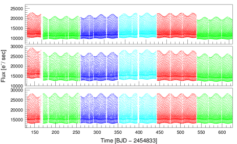
Figure 1.— Top panel: ‘optimal aperture’ flux variation curve of V783 Cyg (Kepler archive). Middle panel: the flux variation curve prepared by using the best tailor-made aperture. Bottom panel: scaled, shifted and detrended curve. (For better visibility, only the first six quarters are plotted.)

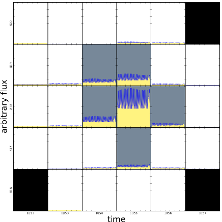
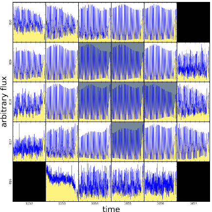
Figure 2.— Constructing of the tailor-made apertures. The entire pixel mask around V783 Cyg (catalog ) (KIC 5559631) in the first quarter. Grey pixels: elements of the ‘optimal apertures’, white pixels: all other downloaded pixels (‘stamp’). We plotted the Q1 time series of each pixel individually. On the left hand side all pixel light curves are scaled between zero and the maximum flux. On the right hand side all pixel light curves are scaled individually. We collected all those pixels that show the signal of the star and omitted those ones which include noise or background sources only.

We assembled our Blazhko star sample in the Kepler field the following way. The sample of Benkő et al. (2010) contains fourteen stars. One of them – V349 Lyr (catalog ) (KIC 7176080) – proved to be a non-modulated star suggested by Nemec et al. (2011). This finding has been confirmed by the present work by checking its pixel photometric data. We also include three additional stars that were analyzed by N13. The extremely small Blazhko effect of V838 Cyg (KIC 10789273) was revealed by N13, while the (Blazhko) RR Lyrae nature of KIC 7257008 (catalog ) and KIC 9973633 (catalog ) was discovered by the ASAS survey (Pojmanski, G. 1997, 2002; Szabó et al. in prep.) when the Kepler measurements had been in progress. That is the reason why we have data on these two targets from Q10 only. The other 13 stars were pre-selected by the Kepler Asteroseimic Science Consortium (KASC) and were observed during the whole mission. N13 shortly noted two additional Blazhko candidates, however, both of those stars are faint ones merging with neighboring bright sources. Because of the serious problems concerning the separation of their signals from their close companions we omitted them from our investigations. (They will be discussed in a forthcoming paper.) RR Lyr (catalog ) itself is also in the Kepler field, but its image is always saturated. Therefore, recovering its original signal needs extra caution and special techniques (e.g. custom apertures). Many successful efforts have been done to this direction (Kolenberg et al., 2010, 2011; Molnár et al., 2012). We will only refer to those results on RR Lyr. Our final sample consists of fifteen Blazhko stars.

The exposition time of the Kepler camera is 6.02 s with 0.52 s readout time. The long cadence (LC) data result from 270 exposures co-added with a total 1766 s integration time. Since we concentrate on long period effects we generally used these LC data only, especially as the time-span of short cadence data (SC: 9 frames codded 58.85 s) are usually no more than one single quarter.

The commissioning phase data (Q0) between 2009 May 2 to 11 (9.7 d) included only one Blazhko star: KIC 11125706 (catalog ). The observations of other targets began with Q1 on 2009 May 13. Here we analyzed LC data to the end of the last full quarter (Q16, till 2013 Apr 8). The total lengths of the data covers 3.9 years. The CCD module No. 3 failed during Q4 (on 2010 January 12), the targets located on this module have quarter-long gaps in their time series data. Six stars of our fifteen-element sample suffer from this defect (see Tab. 3 and Fig. 4). The combined number of data points for a given star is between 19 249 (KIC 9973633) and 61 351 (V783 Cyg), the typical value is about 50-60 000. Data are public and can be downloaded from the web page of MAST.

2.2. Data Processing

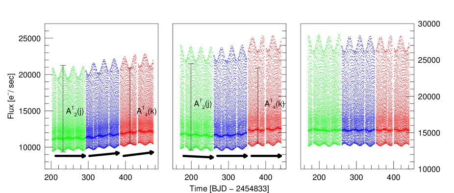
Figure 3.— Flux variation curves from the data processing. The figure shows curves of V783 Cyg from Q2-Q4. From left to the right: the archived Kepler data, fluxes extracted from the best tailor-made apertures, and final rectified data, respectively. The arrows illustrate the internal trends. $A^{\mathrm{T}}_{2}(j)$ and $A^{\mathrm{T}}_{4}(k)$ are the total pulsation amplitude of the archived Kepler Q2 and Q4 data at the $j$th and $k$th pulsation cycles, respectively. These amplitudes are also shown in the tailor-made data plot for comparison.

In this subsection we summarize the main steps done before our analysis. The Kepler data available for each source in two forms (1) as photometric time series: flux variation curves (flux vs. time) prepared from the pre-defined optimal apertures and (2) image time series (image of the stamp vs. time). Latter data sets are often referred to as ‘pixel data’. For the above mentioned reasons we used these pixel data. After we downloaded them from the MAST web page PyKE routines provided by Kepler Guest Observer Office were used to extract the flux variation curves for each pixel in the stamps of a given star. Since the pixel files before file version 5.0 have a time stamp error we corrected it by using the PyKE keptimefix tool.

Table 1Sample from a rectified data file

No	Time	Flux	Zero point offset	Scaling factor	Corrected flux	Corrected Kp
	(BJD$-$2454833)	(e-s-1)	(e-s-1)		(e-s-1)	(mag)
1	131.5123241	5322.6	$-400.00$	1.000	5402.03436789	0.39793763
2	131.5327588	5393.9	$-400.00$	1.000	5473.33140201	0.38370163
3	131.5531934	5496.7	$-400.00$	1.000	5576.12843615	0.36349907
4	131.5736279	5498.1	$-400.00$	1.000	5577.52547030	0.36322708
5	131.5940625	5488.2	$-400.00$	1.000	5567.62250444	0.36515654
6	131.6144972	5571.6	$-400.00$	1.000	5651.01953856	0.34901397
7	131.6349317	6347.2	$-400.00$	1.000	6426.61657271	0.20937502
8	131.6553663	8478.6	$-400.00$	1.000	8558.01360685	$-0.10160144$
9	131.6758010	14437.0	$-400.00$	1.000	14516.41064097	$-0.67531712$
10	131.6962356	15817.5	$-400.00$	1.000	15896.90767511	$-0.77395064$
$\cdots$	$\cdots$	$\cdots$	$\cdots$	$\cdots$	$\cdots$	$\cdots$

We investigated the flux variation curves of all individual pixels separately. We illustrate this process in Fig. 2. Here the stamp of Q1 around the star V783 Cyg (KIC 5559631) is plotted on two different scales. The gray pixels symbolize the elements of the pre-defined ‘optimal’ aperture. We plotted the Q1 time series of each pixel individually. On the left panel all pixel flux variation curves are scaled between zero and the maximum flux attained by the brightest pixel in the stamp. This option shows the relative contribution to the archived flux variation curve by each pixel. The total flux of the star comes obviously from a few pixels only. On the right panel all individual pixel flux variation curves are scaled separately between their minima and maxima to ensure the largest dynamic range for each pixel. This map reveals that there is some flux from outside of the original (‘optimal’) aperture.

Aiming for apertures for each star and quarter separately which include the total flux, we built the ‘tailor-made’ apertures in the following way: if the flux variation curve of a pixel showed the signal of the given variable star – that is the main pulsation period is detectable ($A(f_{0})\sim 3\sigma$) in the Fourier spectrum – we added the pixel in question to our tailor-made aperture, otherwise we dropped it.

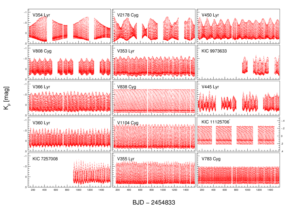
Figure 4.— The gallery of Kepler Blazhko stars. The figure shows the complete light curves of fifteen stars observed with long–cadence (LC) sampling during the periods Q0 through Q16. The light curves are ordered by the primary Blazhko period from the longest (top left) to the shortest (bottom right) ones. ^∗For better visibility the scale of KIC 11125706 is increased by a factor of 1.5.

By summing up the flux of all pixels in the tailor-made apertures we obtained raw flux variation curves.

At first sight these time series and the Kepler flux variation curves do not differ too much (see Fig. 1 for an example). Nevertheless, the difference between the flux values of the archived (‘optimal’ aperture) data and our (‘tailor-made’ aperture) fluxes is considerable: about 1-5 per cents. The exact value differs from star to star and quarter to quarter. We note that such a comparison needs shifting the quarters pairwise to a common zero point.

The main differences between the archived and our flux variation curves are that (i) the total pulsation amplitudes $A^{\mathrm{T}}_{i}(n)$ increase for all quarters ($A^{\prime\mathrm{T}}_{i}(n)>A^{\mathrm{T}}_{i}(n)$; Fig. 3) indicating the flux loss in the archived data. Here the amplitudes $A^{\mathrm{T}}_{i}(n)$, $A^{\prime\mathrm{T}}_{i}(n)$ are the total pulsation amplitude (maximal flux $-$ minimal flux) of the $n$th pulsation cycle in the $i$th quarter $i,n=1,2,\dots$ for optimal and tailor-made aperture data, respectively. (The superscript T stands for the word ‘total’.) (ii) The internal trends within quarters (see arrows in Fig. 3) decrease, suggesting that these trends originate from the small drift and differential velocity aberration of the telescope; and (iii) the difference of the total pulsation amplitudes between the consecutive quarters $\Delta A^{\mathrm{T}}_{i,i+1}=|A^{\mathrm{T}}_{i}(l)-A^{\mathrm{T}}_{i+1}(1)|$ decrease: $\Delta A^{\mathrm{T}}_{i,i+1}>\Delta A^{\prime\mathrm{T}}_{i,i+1}$, (the index $l$ denotes the last pulsation cycle in the $i$th quarter). In an optimal case – if the tailor-made apertures capture all the flux – these total pulsation amplitude differences practically disappear and only zero point shifts would remain between quarters.

Initially we hoped that we could define tailor-made apertures for all stars which include the total flux, i.e. the different quarters can be joined smoothly by simple zero point shifts. We have found such apertures for nine Blazhko stars, only. Six of our stars, however, show total pulsation amplitude differences between quarters for all possible apertures. (For the list of the individual stars see Table 3.) In these cases the downloaded stamps seemed to be too small. The right panel in Fig 2 demonstrates such a situation well: the top pixel row and the right-most column contain the signal of the variable star while e.g. bottom row does not.

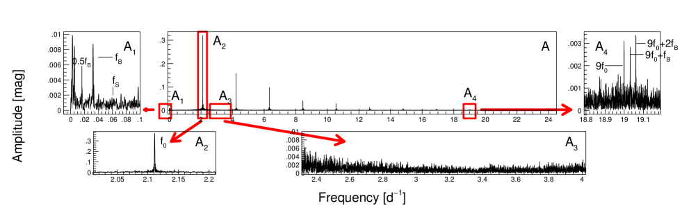
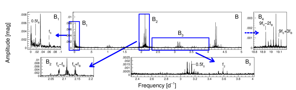
Figure 5.— Schematic overview of the Fourier analysis of the light curves. Top panels (signed by A): Fourier amplitude spectra, bottom panels (signed by B) spectra after we pre-whitened the data with the main pulsation frequency $f_{0}$ and its significant harmonics $kf_{0}$, $k=1,2,\dots$. Panels with indexed letters: zooms of the the spectra, (1) low frequency range, (2) surrounding of $f_{0}$, (3) additional frequencies between $f_{0}$ and $2f_{0}$, (4) high frequency range (around $9f_{0}$). Colored boxes in the middle panels show the approximate positions and sizes of the small (zoomed) panels.

How can we correct the flux variation curve of such stars? Simple zero point shifts do not result in continuous light curves, however, we must assume that the light curve of an RR Lyrae star is continuous and smooth. To this end, we have to scale the flux values for properly joining the quarters. Since at the beginning of the mission, Q4 was the most stable quarter (see fig. 10 in Jenkins et al. 2013) we chose its fluxes as a reference for all stars. We defined scaling factor and zero point offset pairs for each quarter separately so that the transformed flux values of quarters can be stitched smoothly. These transformations are neither exact nor unique. An additional trouble arises when one quarter of data is missing. In those cases, since the stamps of a star were generally fixed for the identical telescope rolls (viz. settings for Q1=Q5=Q9,$\dots$; Q2=Q6=Q10,$\dots$ etc.), we used scaling factor and zero point offset of the previous quarter at the same telescope positions: e.g. if Q8 data are missing we use parameters of Q5 for Q9. It must be kept in mind that this procedure may influence the final result especially when we investigate amplitude changes.

The flux values of each quarter were (1) shifted with zero point offsets and (2) multiplied by scaling factors. Finally, (3) the eventual long time-scale trends were removed from the flux variation curves by a trend filtering algorithm prepared for CoRoT RR Lyrae data and (4) fluxes were transformed into a magnitude scale, where the averaged magnitude of each star was set to zero. We have to emphasize that due to the logarithmic nature of the magnitude scale all corrections and transformations should be performed on the flux data. The measured fluxes fell between 1190 and 350 500 e^-s^-1 which yields the estimated error $7.2\times 10^{-4}$ and $4.2\times 10^{-5}$ mag for an individual data point, respectively. Corrected time series data on the tailor-made apertures are available both in flux and magnitude scales in electronic format. The fluxes extracted from the tailor-made aperture without trend filtering, applied scaling factors and offset values are also given in the data set (for a sample see Table 1).

3. Analysis and Results

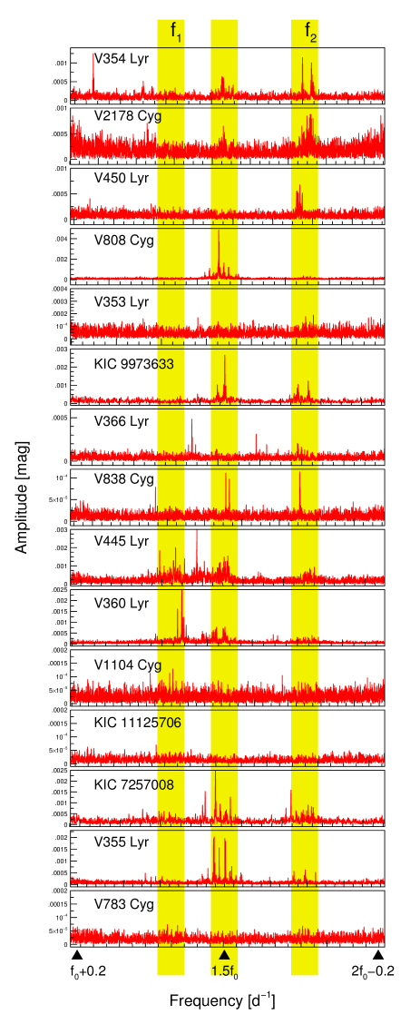
Figure 6.— Structure of the additional frequencies. Here we plotted the spectra between the main frequencies and their first harmonics ($f_{0}+0.2<f<2f_{0}-0.2$). All figures show residual spectra after consecutive pre-whitening steps with the harmonics and their numerous (3-10) significant side peaks. The yellow stripes indicate the expected position of the radial first overtone ($f_{1}$), period doubling ($1.5f_{0}$) and radial second overtone ($f_{2}$) frequencies, respectively.

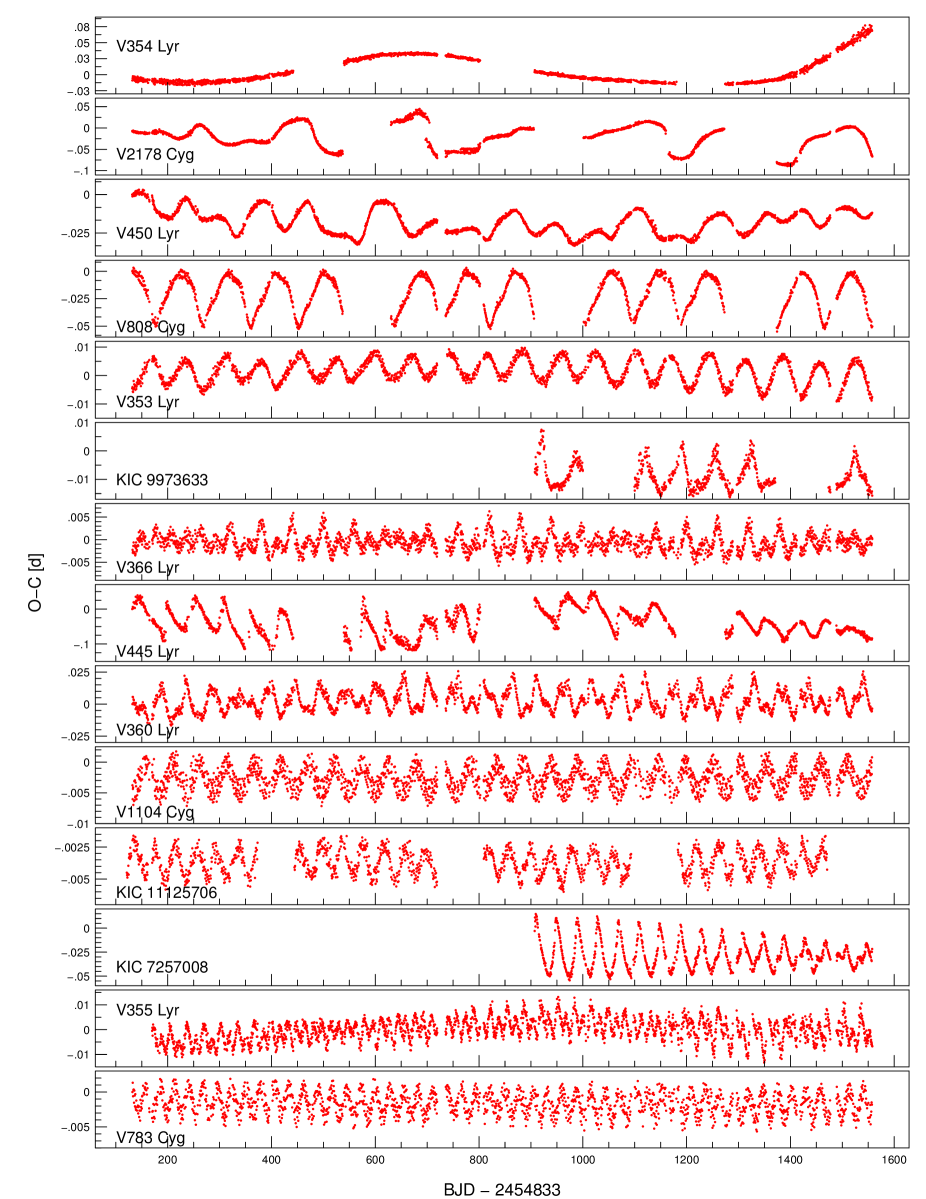
Figure 7.— The O$-$C diagrams of the analyzed Blazhko RR Lyrae stars. The diagrams are constructed from interpolated times of pulsation maxima. The basic epochs are the times of the first maximum for all stars. The primary AM Blazhko period decreases from top to bottom. The LC data of V838 Cyg is not suitable for constructing the O$-$C diagram (for the details see Sec. 3.2.13), so it has not shown here.

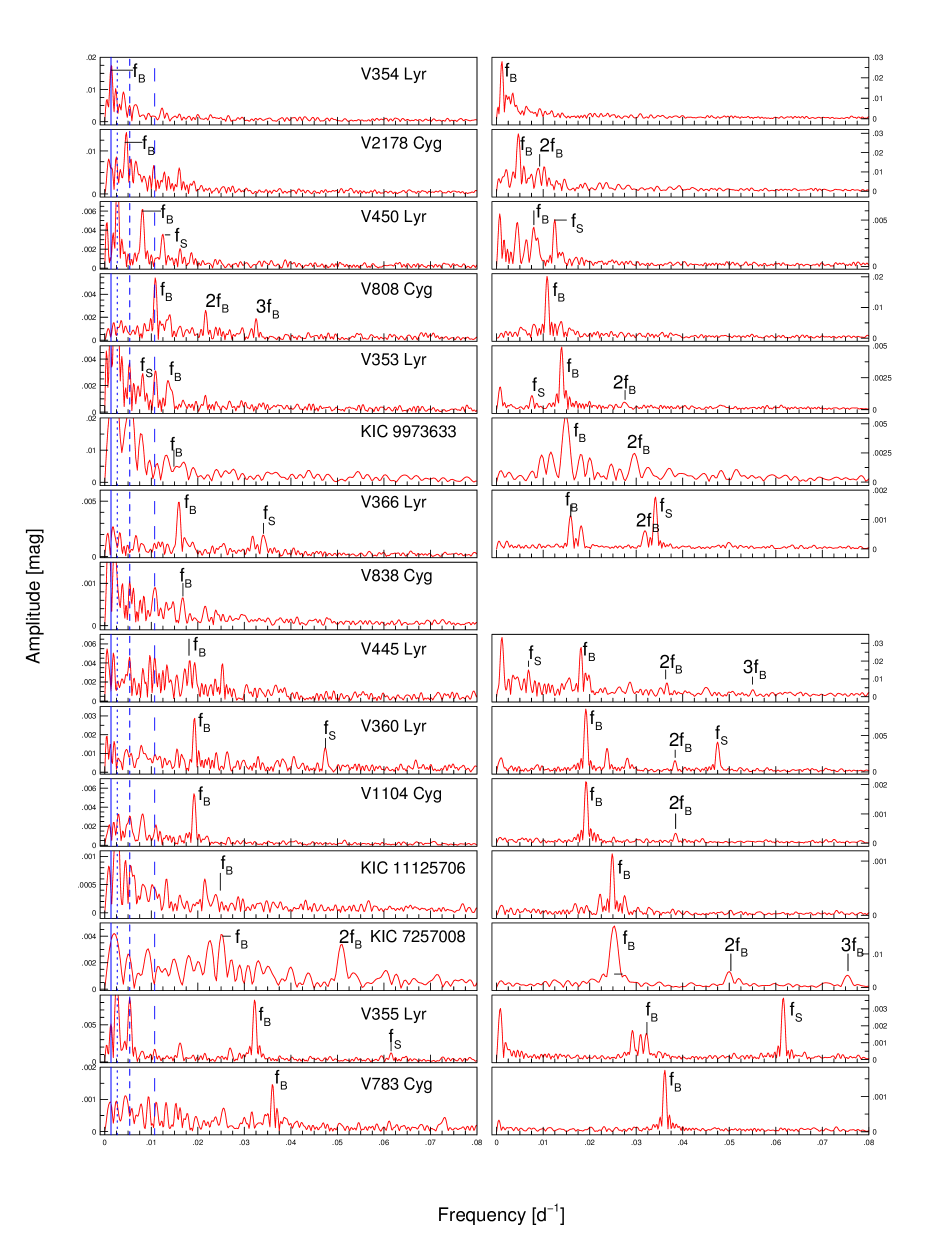
Figure 8.— Properties of amplitude and frequency modulations. Left panels: low frequency range of the Fourier spectra of the light curve (Fig. 4). Blue vertical lines show the location of the common instrumental frequencies: $f_{\mathrm{K}}/2$ (continuous), $f_{\mathrm{K}}$ (dotted), $2f_{\mathrm{K}}$ (short dashed), $4f_{\mathrm{K}}=f_{\mathrm{Q}}$ (long dashed), respectively. Right panels: Fourier spectra of the O$-$C diagrams (Fig. 7). For both cases the primary ($f_{\mathrm{B}}$) and secondary modulation frequencies ($f_{\mathrm{S}}$) and their harmonics are marked. Possible linear combinations are shown in Figs. 14 and 15.

3.1. General Overview

In the course of this study we mainly used two methods. One of them is the Fourier analysis of the light curves that were pre-conditioned by the described process and shown in Fig. 4. The second method is the analysis of O$-$C (observed minus calculated) diagrams. In some cases other tools were used, as well. These are described later when we discuss the relevant objects.

This paper uses the following notation conventions: numbers in the lower indices denote the radial pulsation orders (viz. 0 = fundamental, 1 = first overtone modes, etc.). Lower indices B and S indicate the primary (Blazhko) and secondary modulations, respectively. Upper indices denote the detected frequencies before identification. Throughout this paper the numerical values (frequencies, amplitudes, etc.) are written with the significant number of digits plus one digit.

3.1.1 Fourier Analysis of the Light Curves

The software packages MuFrAn (Kolláth, 1990) and Period04 (Lenz & Breger, 2005) were used for the Fourier analysis. These program packages – together with SigSpec (Reegen, 2007) – were tested for Kepler Blazhko stars in the past (Benkő et al., 2010). Since all of them provided similar spectra with the same frequencies, amplitudes and phases we can use the one which fits the best our purposes. In this work our primary tool was MuFrAn, but e.g. the frequency error or signal-to-noise ratio (S/N) were determined by Period04.

Here we describe the general features of our Fourier analysis. For an illustration see Fig. 5. The highest peaks in the Fourier spectra are always the main pulsation frequencies ($f_{0}$) and their harmonics ($kf_{0}$, where $k=1,2,\dots$) (see panel A in Fig. 5). The Nyquist frequency for the Kepler LC data is $f_{\mathrm{N}}=24.46$ d^-1. Up to this limit frequency we detected 9-15 significant harmonics depending on the pulsation frequency.

When we pre-whiten the data with these frequencies, we get Fourier spectra dominated by the side peaks (Fig. 5B). The harmonics (including the main frequency) are surrounded by the side peaks caused by the Blazhko modulation ($kf_{0}\pm lf_{\rm B}$, where $k,l=1,2,\dots$). Side peaks of triplets ($l=1$) can always be seen (panel B₂ in Fig. 5) and in some cases higher order multiplets ($l>1$) are also detectable (panel B₄). The higher order multiplets tend to appear around the higher order harmonics which indicates the frequency modulation (Benkő, Szabó & Paparó, 2011).

After we pre-whitened the data with a set of side frequencies it turned out to be evident that the side peaks sometimes consist of double or even multiple peaks. If we measure the spacing between these double peaks we find that the frequency difference corresponds to the Kepler year ($P_{\rm K}=372.5$ days). More precisely, these frequencies can be described as $kf_{0}\pm f^{\prime}$, where $f^{\prime}$ is one of the followings: $0.5f_{\rm K}$, $f_{\rm K}$, $2f_{\rm K}$, $4f_{\rm K}=f_{\rm Q}$. Here $f_{\rm K}=1/P_{\rm K}$ and $f_{\rm Q}=1/P_{\rm Q}$, where $P_{\rm Q}$ is the characteristic length of a quarter. Thus these frequencies are caused either by not properly eliminated problems of stitched quarters, missing quarters or sometimes the instrumental amplitude variation with $P_{\rm K}$ recently discovered by Bányai et al. (2013).

In the low frequency ranges (panel B₁ in Fig. 5 and Fig 8) we generally find the modulation frequencies $f_{\rm B}$, frequencies connected to the Kepler year, and some other instrumental peaks. In many cases we also find the harmonics of the Blazhko frequencies to be significant. It implies that the amplitude modulation is fairly non-sinusoidal which is evident from the envelopes of the corresponding light curve in Fig. 4. It is surprising that in many cases more than one modulation peaks can be found (see also B₁ in Fig. 5). These secondary modulation frequencies sometimes mimic to be the harmonic of the primary modulation frequencies but the O$-$C analysis (see Sec. 3.1.2) helped us to distinguish multiple modulation and non-sinusoidal modulation. The ratios between different Blazhko frequencies are often close to small integer numbers, which may suggests a resonance at work.

Although this paper focuses on the long time-scale variations, we briefly discuss the frequency ranges between the harmonics, since the spectra after pre-whitening with the modulation frequencies and the side peaks show specific structures (see panel B₃ in Fig. 5). Four stars (V353 Lyr (catalog ), V1104 Cyg (catalog ), KIC 11125706 and V783 Cyg) do not show any significant peaks in these frequency ranges, but the remaining eleven stars do (Fig. 6).

Three well separated forests of peaks can be identified which appear in all stars with different combinations. The middle ones belong to the period doubling (PD) phenomenon (Kolenberg et al., 2010; Szabó et al., 2010; Kolláth, Molnár & Szabó, 2011). The half-integer frequencies (HIFs: $0.5f_{0},1.5f_{0},\dots$), their side peaks and a number of linear combination frequencies can be detected. If we determine the frequency ratio of these HIF peaks we find that their values frequently differ from the exact half-integer ratios. The explanation is a combination of mathematical, physical and sampling effects (Szabó et al., 2010). The frequencies located between the HIFs and $2f_{0}$ harmonics belong to the second radial overtone ($f_{2}$), while peaks between $f_{0}$ and HIFs are identified as the frequency of the first radial overtone mode ($f_{1}$). The explanation of the huge number of surrounding peaks around all three cases is mathematical: the amplitude of the additional frequencies for both the PD effect and overtone modes changes in time (see e.g. Benkő et al. 2010; Szabó et al. 2010, 2014; Guggenberger et al. 2012). Such a variable signal results in a forest of peaks in the Fourier spectra as it was shown by Szabó et al. (2010).

3.1.2 Analysis of the O$-$C Diagram

The FM part of the Blazhko effect can be separated if we study the effect in the time domain. Since the AM and FM definitely connected to each other, such an investigation shows different aspects of the same phenomenon. A practical advantage of this handling is that the time measurements are almost free of instrumental problems contrary to the brightness measurements which were discussed in Sec. 2.

There are numerous opportunities for following frequency/period variations from the traditional O$-$C diagram (Sterken, 2005) to the analytic signal method (Kolláth et al., 2002) or we can transform it to phase variation as e.g. N13. We have chosen here the O$-$C diagram analysis as a simple and clear method. Although O$-$C diagrams were widely used for investigating RR Lyrae stars for many decades, the first diagrams that show the period variations due to the Blazhko effect were published only recently (Chadid et al., 2010; Guggenberger et al., 2012), when the continuous space-based data became available.

As Sterken (2005) defined “O$-$C stands for O[bserved] minus C[alculated]: … it involves the evaluation and interpretation of the discord between the measure of an observable event and its predicted or foretold value.” In our case we chose the time of maxima of the pulsation as an “observable event”. For the determination of the observed maximum times (‘O’ values) we used 7-9th order polynomial or spline fits around the maximum brightness of each pulsation cycle. The initial epochs ($E_{0}$) were always the time of the first maximum for each star. The ‘C’ (calculated) maximum times were determined from these epochs and the averaged pulsation periods ($P_{0}$): C=$E_{0}+EP_{0}$, where $E=1,2\dots$, is the cycle number. Gaps in the observed light curves often resulted in interpolation errors and consequently deviant points in the constructed O$-$C curves. We removed these points with the time string plot tool of Period04. The selection criterium for the wrong points was that they deviate from the smooth fit of the curves more than $3\sigma$, where $\sigma$ indicates the standard deviation of the fit. The obtained curves are plotted in Fig. 7. The accuracy of an individual O$-$C value is about 1 minute.

The frequency content of the O$-$C diagrams were extracted again by Fourier analysis. The corresponding spectra are shown in Fig. 8, where we compare them with the low frequency range of the light curve Fourier spectra. Generally speaking the structures of these two types of spectra are similar, but O$-$C spectra are more clear. Here no instrumental peaks can be detected and in the case of multiple modulated stars the linear combination frequencies are also more numerous and significant. These linear combination frequencies demonstrate that both modulations belong to the same star (and not to a background source) and the nonlinear coupling between different modulations. It is noteworthy that the frequencies of the AM and FM are always the same within their errors.

Table 2Blazhko periods and amplitudes from different methods

Name	$P^{\mathrm{(s)}}_{i}$	$P^{\mathrm{AM}}_{i}$	$A(f^{\mathrm{AM}}_{i})$	$P^{\mathrm{FM}}_{i}$	$A(f^{\mathrm{FM}}_{i})$
	[d]	[d]	[mmag]	[d]	[min]
V2178 Cyg	$207\pm 15$	$216\pm 2$	$14\pm 3.7$	$215.9\pm 0.35$	$43.6\pm 0.9$
	$168.8\pm 1.1$			$166.2\pm 2.4$	$18.6\pm 1.2$
V808 Cyg	$92.14\pm 0.06$	$92.18\pm 0.39$	$5.4\pm 0.7$	$92.16\pm 0.01$	$30.6\pm 0.1$
V783 Cyg	$27.666\pm 0.001$	$27.73\pm 0.39$	$1.5\pm 1.2$	$27.667\pm 0.005$	$2.6\pm 0.05$
V354 Lyr	$807\pm 16$			$891\pm 4$	$36.9\pm 0.5$
V445 Lyr	$54.7\pm 0.5$	$54.80\pm 0.3$	$4.3\pm 1.2$	$55.04\pm 0.04$	$38.7\pm 1.5$
	$146.4\pm 0.8$			$147.4\pm 0.7$	$21.8\pm 1.7$
KIC 7257008	$39.51\pm 0.05$	$39.7\pm 0.4$	$4.2\pm 1.9$	$39.72\pm 0.02$	$26.3\pm 0.4$
V355 Lyr	$31.06\pm 0.1$	$31.04\pm 0.08$	$8.4\pm 1.8$	$30.99\pm 0.02$	$2.3\pm 0.1$
	$16.243\pm 0.007$	$16.25\pm 0.1$	$1.2\pm 1.7$	$16.229\pm 0.003$	$5.2\pm 0.1$
V450 Lyr	$123.7\pm 0.4$	$123.0\pm 1$	$6.5\pm 1.4$	$124.8\pm 0.3$	$5.7\pm 0.3$
	$81.0\pm 0.6$	$80.4\pm 0.8$	$4.3\pm 1.5$	$80.1\pm 0.1$	$6.7\pm 0.3$
V353 Lyr	$71.70\pm 0.04$	$72.1\pm 1.5$	$2.3\pm 1.3$	$71.68\pm 0.02$	$7.17\pm 0.07$
	$133.1\pm 0.4$			$131.3\pm 0.3$	$1.64\pm 0.08$
V366 Lyr	$62.90\pm 0.01$	$62.87\pm 0.4$	$5.0\pm 1.4$	$62.77\pm 0.05$	$1.66\pm 0.06$
	$29.29\pm 0.01$	$29.28\pm 0.3$	$2.1\pm 1.4$	$29.295\pm 0.007$	$2.58\pm 0.06$
V360 Lyr	$52.10\pm 0.01$	$51.88\pm 0.5$	$2.9\pm 1.2$	$52.11\pm 0.015$	$12.9\pm 0.2$
	$21.041\pm 0.008$	$21.09\pm 0.15$	$1.3\pm 1.2$	$21.073\pm 0.005$	$6.0\pm 0.2$
KIC 9973633	$67.11\pm 0.08$			$67.30\pm 0.07$	$8.2\pm 0.2$
	$27.13\pm 0.06$			$27.21\pm 0.15$	$1.6\pm 0.4$
V838 Cyg	$59.5\pm 0.1$	$59.8\pm 3$	$0.6\pm 2$
KIC 11125706	$40.21\pm 0.02$			$40.21\pm 0.01$	$1.66\pm 0.03$
				$58.9\pm 0.1$	$0.27\pm 0.03$
V1104 Cyg	$52.00\pm 0.01$	$52.08\pm 0.2$	$5.4\pm 1.8$	$51.99\pm 0.02$	$3.14\pm 0.05$

3.1.3 Calculated Parameters and Accuracies

Figure 9.— Blazhko period(s) vs. amplitude of the AM frequency. For the plotted values see Table 2.

The analyzed Fourier spectra have well-defined structures and although the spectra of the light curves contain hundreds of significant peaks, only few of them belong to independent frequencies. These are the main pulsation frequency $f_{0}$, the Blazhko frequencies ($f_{\mathrm{B}}$ and $f_{\mathrm{S}}$) and the frequencies of the excited additional radial overtone mode(s) ($f_{1}$, $f_{2}$ and/or the strange mode $f_{9}$ which responsible for the PD effect). The error estimation for both the frequencies and amplitudes were obtained by Monte Carlo simulation of Period04. We note that these errors are only few percents higher than the analytic error estimations (Breger et al., 1999), because we have almost continuous and uniformly sampled data sets.

The error estimation of the main pulsation frequency yields 1.1-1.8$\times 10^{-7}$ d^-1 for the Q1-Q16 data sets while 4$\times 10^{-6}$ d^-1 for the Q10-Q16 data. These translate to 3-5$\times 10^{-8}$ d period uncertainty for the best data (short period and long observing span) and $10^{-6}$ d at worst. The Rayleigh frequency resolution is 0.0007 d^-1 for Q1-Q16 data sets, and 0.0015 d^-1 for Q10-Q16 data (for KIC 7257008 and KIC 9973633). The frequencies never change due to a modulation (Benkő, Szabó & Paparó, 2011) as opposed to the amplitudes which are affected by the FM. Consequently, our formal error estimation for the main pulsation amplitudes (0.3-1 mmag) are lower limits only.

The Blazhko periods were determined by three different ways (see Table 2): (i) from the averaged frequency differences of the first two triplets (second column); (ii) from the Blazhko frequencies themselves (column 3) – if they are detectable in the spectrum of the light curve – and (iii) from the Fourier spectrum of the O$-$C diagrams (column 5). The latter two methods provide the AM and FM amplitudes which are shown in columns 4 and 6 in Table 2.

We call the attention of the reader to an interesting phenomenon. In Fig. (9) we plot the Blazhko period ($P_{i}$) vs. amplitude of the AM frequency ($A(f^{\mathrm{A}M}_{i})$) diagram, where $i$=B or S. We find a trend: the longer Blazhko periods mean larger amplitudes and vice verse. We can not rule out that this is a small sample effect, however, some arguments contradict to this scenario. The emptiness of the long period and small amplitude part of the diagram can be explained by observational effect (it is difficult to distinguish between small-amplitude long-period stellar variations and the instrumental effects with similar time-scales even in the Kepler data), but the lack of points of the small period and large amplitude part can not. Additionally, similar effects are common for (hydro)dynamical systems: e.g. weakly dissipating systems could be perturbed for high amplitude by long time-scale perturbing forces only (Molnár et al., 2012). The found effect will be investigated in a separate study.

Basic parameters obtained from this analysis are summarized in Table 3. The columns of the table show the ID numbers and names of the stars, main pulsation periods and their Fourier amplitude where the number of digits indicate the accuracy. Columns 5 and 6 contain the modulation periods averaged from the values in Table 2. The last two columns of the table indicate the presence of additional frequencies, instrumental problems and auxiliary information about the Kepler observations.

Table 3Basic properties of the Kepler Blazhko stars

KIC	GCVS	$P_{\mathrm{0}}$	$A(f_{0})$	$P_{\mathrm{B}}$	$P_{\rm S}$		Add. freq.	remarks
		[d]	[mag]	[d]	[d]
3864443	V2178 Cyg	$0.4869470$	0.3156	$213\pm 5$	$167.5\pm 1.8$(?)		F2, (PD)	m
4484128	V808 Cyg	$0.5478635$	0.2197	$92.16\pm 0.02$	$\sim 1000$		PD, (F2)	m
5559631	V783 Cyg	$0.6207001$	0.2630	$27.6667\pm 0.0005$				scal
6183128	V354 Lyr	$0.5616892$	0.2992	$849\pm 59$	(?)		F2, (PD, F’)	scal, m
6186029	V445 Lyr	$0.5130907$	0.2102	$54.83\pm 0.04$	$146.9\pm 0.7$		PD, F1, F2	m
7257008		$0.511787$	0.2746	$39.67\pm 0.14$	$>900$		PD, F2	Q10-
7505345	V355 Lyr	$0.4736995$	0.3712	$31.02\pm 0.05$	$16.24\pm 0.01$		PD, F2
7671081	V450 Lyr	$0.5046198$	0.3110	$123.8\pm 0.9$	$80.5\pm 0.5$		F2	scal
9001926	V353 Lyr	$0.5567997$	0.2842	$71.8\pm 0.3$	$132.2\pm 1.3$
9578833	V366 Lyr	$0.5270284$	0.2909	$62.84\pm 0.07$	$29.29\pm 0.01$		(F2)
9697825	V360 Lyr	$0.5575755$	0.2572	$52.03\pm 0.14$	$21.07\pm 0.03$		F2, (PD)
9973633		$0.510783$	0.2458	$67.2\pm 0.1$	$27.17\pm 0.06$		PD, F2	m, Q10-
10789273	V838 Cyg	$0.4802800$	0.3909	$59.7\pm 0.2$			(F2, PD)	scal
11125706		$0.6132200$	0.1806	$40.21\pm 0.02$	$58.9\pm 0.1$			m, scal
12155928	V1104 Cyg	$0.4363851$	0.3847	$52.02\pm 0.05$				scal

3.2. Analysis of Individual Stars

3.2.1 V2178 Cyg = KIC 3864443

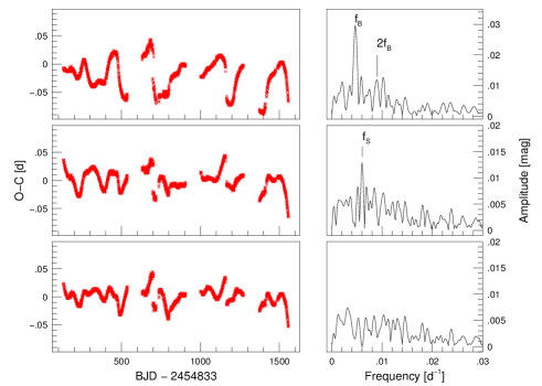
Figure 10.— O$-$C analysis of V2178 Cyg. Left panels show the O$-$C diagram (top) and its residuals after we pre-whitened the data with $f_{\mathrm{B}}$ and $2f_{\mathrm{B}}$ (middle) and also with $f_{\mathrm{S}}$ (bottom). Right panels show the Fourier spectra of the O$-$C data during this consecutive pre-whitening process.

This star was chosen by N13 as a representative of the long period Blazhko stars showing large AM and FM. The envelope of the light curve in Fig. 4 shows complicated amplitude changes suggesting multiperiodicity and/or cycle-to-cycle variations of the Blazhko effect. Unfortunately, the long time-scales of the variations make quantification of this phenomenon impossible. We detected 11 significant harmonics of the main pulsation frequency ($f_{0}$) up to the Nyquist frequency. The triplet structures around the harmonics are highly asymmetric: $A(kf_{0}-f_{\mathrm{B}})\gg A(kf_{0}+f_{\mathrm{B}})$ (see also fig. 3 in N13). If we calculate the primary Blazhko frequency from the averaged spacing of the side peaks we find $0.00482$ d^-1. This value is in good agreement with the highest amplitude peak in the low frequency range ($0.00462\pm 0.0001$ d^-1) so it can be identified with $f_{\mathrm{B}}$ (Fig. 8). Due to the missing quarters the Fourier spectrum contains numerous instrumental frequencies such as $f_{\mathrm{Q}}$, $f_{\mathrm{Q}}\pm f_{\mathrm{B}}$ and their linear combinations with the main frequency and its harmonics. The second largest low frequency peak is at 0.002486 d^-1 which coincides with $f_{\mathrm{K}}=0.002685$ d^-1 within the determination error (0.0001 d^-1).

After we subtracted the largest amplitude side peaks ($kf_{0}-f_{\mathrm{B}}$) in the spectrum of the residual, the other components of the triplets ($kf_{0}+f_{\mathrm{B}}$) and additional side peaks of a possible secondary modulation ($kf_{0}-f_{\mathrm{S}}$) appeared, where $f_{\mathrm{S}}=0.00593$ d^-1. If $f_{\mathrm{S}}$ belongs to a secondary modulation, the ratio of two modulation frequencies would be 2:3, however, $f_{\mathrm{S}}$ can also be interpreted as a linear combination: $f_{\mathrm{S}}=f_{\mathrm{Q}}-f_{\mathrm{B}}$.

When we compute the Fourier spectrum of the O$-$C diagram (Fig. 10) we find $f_{\mathrm{B}}=0.00463$ d^-1 and $2f_{\mathrm{B}}$. Pre-whitening with these frequencies one significant peak appears at 0.00602 d^-1 (S/N=24). If we remove this frequency as well, the residual curve shows large amplitude quasi-periodic oscillations, but no further frequencies can be identified. Our conclusion is that V2178 Cyg shows a multiperiodic and/or quasi-periodic Blazhko effect but the long periods do not allow us to draw final conclusion.

Similarly to Benkő et al. (2010), we found a bunch of peaks around the frequency of the second radial overtone mode (see also in Fig. 6, $f_{2}=3.51478$ d^-1, $P_{0}/P_{2}=0.584$; S/N $\approx 3$). The PD phenomenon is marginal: the highest peak around $1.5f_{0}$ is $f^{(1)}=3.05804$ d^-1 ($f^{(1)}/f_{0}=1.49$; S/N $\approx 2$). A third additional peak condensation can be seen around $f^{(2)}=2.656875$ d^-1 (S/N $\approx 2$). Though some Blazhko stars (e.g. RR Lyr, V445 Lyr (catalog )) show radial first overtone frequency ($f_{1}$) around this region, we could identify this peak of V2178 Cyg as a linear combination $f^{(2)}=3f_{0}-f_{2}$ with high certainty, because the period ratio $P^{(2)}/P_{0}=0.773$ is far from the canonical value of $P_{1}/P_{0}=0.744$. Because this period ratio increases with the increasing metallicity (see e.g. fig. 8. in Chadid et al. 2010) the measured low metallicity of V2178 Cyg ([Fe/H]$=-1.46$, N13) also supports the linear combination explanation.

3.2.2 V808 Cyg = KIC 4484128

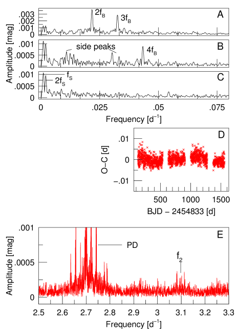
Figure 11.— New results from V808 Cyg. A-C panels: The pre-whitening process of the O$-$C diagram shown in Fig. 7. The harmonics of the Blazhko frequency $f_{\mathrm{B}}$ are significant up to the 4th order. A long time-scale variation is evident because of the presence of low frequency peaks ($f_{\mathrm{S}}$, $2f_{\mathrm{S}}$) and side frequencies around the harmonics of $f_{\mathrm{B}}$. Panel D: residual O$-$C curve containing only $f_{\mathrm{S}}$ and $2f_{\mathrm{S}}$. Panel E: the second radial overtone frequency ($f_{2}$) can be detected from the Q1-Q16 data.

The light curve of this star in Fig. 4 shows two important features. First, the envelope shape suggests a highly non-sinusoidal AM. Second, the length of the Blazhko cycle is close to the length of the observing quarters. As a consequence of the first fact, we can detect two significant harmonics $2f_{\mathrm{B}}$ and $3f_{\mathrm{B}}$ of the Blazhko frequency $f_{\mathrm{B}}=0.01085$ d^-1 (Fig. 8), and multiplet side peaks ($kf_{0}\pm lf_{\mathrm{B}}$, where $l>1$) are detectable, as well. A slight cycle-to-cycle amplitude change might be present but the quarter-long Blazhko period and gaps together make such an effect barely detectable.

The O$-$C diagram of V808 Cyg (catalog ) can be fitted well with the Blazhko period and its three harmonics. After we subtracted this four-frequency fit from the O$-$C data, a definite structure can be detected in the residual spectrum (panel B in Fig. 11). At the position of $f_{\mathrm{B}}$ and $3f_{\mathrm{B}}$ side peaks appear. These peaks define a secondary modulation with the frequency of $f_{\mathrm{S}}=0.0010$ d^-1. The pre-whitened spectrum indeed shows two peaks at $f_{\mathrm{S}}$ and $2f_{\mathrm{S}}$ (panel C). However, the possible period $P_{\mathrm{S}}\sim 1000$ d is commensurable with the length of the total observational time, so this O$-$C variation in panel D could be secular, as well.

V808 Cyg shows the strongest known PD effect that is why data taken during the first two quarters were investigated in detail by Szabó et al. (2010). Using the time series up to Q16 this main finding remains unchanged. The highest amplitude HIF is at $1.5f_{0}$, namely $f^{(1)}=2.69770$ d^-1 ($f^{(1)}/f_{0}=1.48$; S/N $\approx 30$). After applying a few-step pre-whitening process – when we subtract the main pulsation frequency, its harmonics and some (6-10) significant multiplets around the harmonics – we found that the second radial overtone mode (or a non-radial mode at the location of the radial one) $f_{2}=3.09774$ d^-1 ($P_{2}/P_{0}$=0.589) is also excited (panel E in Fig. 11). The amplitude of this frequency is much lower than the amplitudes of the PD frequencies, which explains why previous investigations have not discovered this mode.

3.2.3 V783 Cyg = KIC 5559631

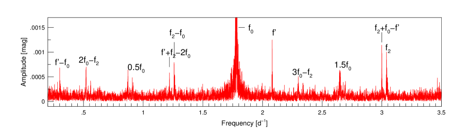
Figure 12.— Additional peaks in the lower frequency range of the pre-whitened Fourier spectrum of V354 Lyr light curve.

The Blazhko effect of V783 Cyg seems to be simple: a sinusoidal AM and FM visible both in the light curve (Fig. 4) and O$-$C diagram (Fig. 7). By investigating these curves more carefully we can detect small differences between consecutive cycles.

When we pre-whiten the light curve data with the main pulsation frequency and its 15 significant harmonics we find nice symmetric triplet structures in the spectrum around the harmonics. The star has the shortest Blazhko cycle in our sample ($P_{\mathrm{B}}=27.67$ d). The spectrum also contains the modulation frequency itself: $f_{\mathrm{B}}=0.036058$d^-1. After subtracting the triplets in the residual spectrum, multiplet side frequencies appear. By carrying out a similar few-step pre-whitening process as in Sec. 3.2.2 we can eliminate all side peaks and no additional peaks emerge between the harmonics.

Fourier analysis of the O$-$C diagram provides us $f_{\mathrm{B}}$ again (Fig. 8). When we subtract a fit with $f_{\mathrm{B}}$, the residual O$-$C diagram shows a parabolic shape indicating a period change. Fitting a quadratic function in the form

$$\mathrm{O}-\mathrm{C}=\frac{1}{2}\frac{dP_{0}}{dt}\bar{P_{0}}E^{2}$$

(Sterken, 2005), where $\bar{P_{0}}$ means the averaged period, $E$ the cycle number from the initial epoch, we find a period increase: $dP_{0}/dt=1.02\times 10^{-9}\pm 1.7\times 10^{-10}$ dd^-1. That is $0.12\pm 0.02$ dMy^-1 which agrees well with the value of Cross (1991) $0.088\pm 0.023$ dMy^-1, who determined it on the basis of photometric observations between 1933 and 1990.

The Fourier analysis of the light curve and O$-$C diagram are not sensitive for the mentioned slight cycle-to-cycle variation of the Blazhko effect. The short Blazhko period and uninterrupted Kepler data make V783 Cyg a good candidate for a dynamical analysis. This study will be discussed in a separate paper by Plachy et al. (in prep.). The preliminary results suggest that the cycle-to-cycle variation of V783 Cyg light curve and O$-$C diagram have chaotic nature.

3.2.4 V354 Lyr = KIC 6183128

The star has the longest Blazhko period in the Kepler sample. We find $P_{\mathrm{B}}=807$ d ($f_{\mathrm{B}}=0.00124$ d^-1) calculating from the triplet spacing in the spectrum of the light curve. At the same time the highest peak in the low frequency range is at $f_{\mathrm{B}}=0.00134$ d^-1 which yields $P_{\mathrm{B}}=748$ d. The problem is that the Blazhko period is inseparably close to the instrumental period $2P_{\mathrm{K}}=745$ d.

The observed two Blazhko cycles in Fig. 4 look different. The ascending branch of the first cycle is steeper than that of the second one while the descending branch of the second cycle is the steeper. The different shapes of the two cycles in the O$-$C diagram (Fig. 7) strengthen our suspicion: V354 Lyr (catalog ) shows multiperiodicity or cycle-to-cycle variations in the Blazhko effect. The long Blazhko period prevents us from quantifying this feature.

As it was already found by Benkő et al. (2010), the Fourier spectrum of V354 Lyr contains significant additional peaks between harmonics. The following frequencies were reported between $f_{0}$ and $2f_{0}$ (with the notations of the referred paper): $f^{\prime}=2.0810$, $f^{\prime\prime}=2.4407$, $f^{\prime\prime\prime}=2.6513$ and $f_{2}=3.03935$ d^-1. After we removed the main pulsation frequency, its significant harmonics, and the highest amplitude side peaks around the harmonics, our spectrum (Fig. 12) also contains numerous additional frequencies. The highest amplitude peak from the half-integer frequency is located now at $f^{(1)}=2.648387=1.5f_{0}$ ($f^{(1)}/f_{0}$=1.49). Identifying the frequency of the radial second overtone mode is problematic, because there is a double peak in that position: $f^{(1)}_{2}=3.038671$ d^-1 ($P^{(1)}_{2}/P_{0}=0.586$) and $f^{(2)}_{2}=2.999333$ d^-1 ($P^{(1)}_{2}/P_{0}=0.593$). The spacing between these two frequencies is 0.300d^-1. Similar double peak structures can be seen for many other frequencies.

The highest amplitude additional frequency $f^{\prime}=2.080672$ d^-1 is mysterious. We have not found any frequencies in such a position for other Blazhko stars (see also Fig. 6). Neither known instrumental frequencies nor linear combinations of instrumental and real frequencies give peak at this position. The spectral window function has a comb like structure (Van Cleve et al., 2009), but the peaks are far from $f^{\prime}$ and their amplitude are very low (in a normalized scale $\sim 0.004$). So we can rule out $f^{\prime}$ being an instrumental frequency.

We checked whether this frequency comes from this star or not. Using the flux data we searched for its linear combination frequencies with the main pulsation one. Both the $f^{\prime}+f_{0}=3.8613$ d^-1 and $f^{\prime}-f_{0}=0.3003$ d^-1 are indeed detectable. So we could rule out a background star as the source of this frequency. The period ratio is $P^{\prime}/P_{0}=0.855$. Benkő & Szabó (2014) raised an explanation that this frequency would be a linear combination of the main pulsation $f_{0}$ and radial first overtone mode frequencies $f_{1}$, namely $f^{\prime}=(f_{0}+f_{1})/2$. The problem of this interpretation is that the spectrum shows significant peaks neither at $f_{0}+f_{1}$ nor at $f_{1}$.

As we have seen the spacing between $f^{(1)}_{2}$ and $f^{(2)}_{2}$ can be given as $f^{\prime}-f_{0}$, so any of them can be calculated as a linear combination of $f_{2}$, $f_{0}$ and $f^{\prime}$. In Fig. 12 we identified $f_{2}=f^{(1)}_{2}$, therefore $f^{(2)}_{2}=f_{2}+f_{0}-f^{\prime}$. Alternatively, if we identify $f_{2}=f^{(2)}_{2}$, then $f^{(1)}_{2}=f_{2}+f^{\prime}-f_{0}$. We can find several other peaks where we have alternate identifications depending on how we choose $f_{2}$.

The last frequency listed by Benkő et al. (2010) is $f^{\prime\prime}=2.4407$ d^-1. Although this frequency is not significant in the spectrum calculated from Q1-Q16 data, but the half of it (1.220 d^-1) can be detected. The later frequency can easily be produced by $f_{2}-f_{0}$ if we identify $f_{2}=f^{(2)}_{2}$. As we have shown in Benkő & Szabó (2014) frequency combination $2(f_{2}-f_{0})$ could explain numerous previously unidentified peak in spectra of some CoRoT and Kepler Blazhko stars. So it is not surprising that we temporarily detect this combination frequency $2(f_{2}-f_{0})=2.4407$ d^-1 in V354 Lyr, as well. As we mentioned in Sec. 3.1.1 all additional frequency amplitudes (HIFs, overtones) change in time, these combination frequencies also seem to show similar time dependency.

3.2.5 V445 Lyr = KIC 6186029

The light curve of the star shows strong and complicated amplitude changes (Fig. 4). It was the subject of a detailed study of Guggenberger et al. (2012). The paper used the data available in that time (Q1-Q7), but its main statements are not changed in the light of the more extended Q1-Q16 data set. The heavily varying parameters such as the different periods, amplitudes and phases result in a slightly different averaged values for these parameters compared to ones given by Guggenberger et al. (2012). We confirm the existence of two modulation frequencies ($f_{\mathrm{B}}$, $f_{\mathrm{S}}$) and four additional frequency patterns, namely $f_{2}$, $f_{1}$, PD and $f_{\mathrm{N}}=2.763622$ d^-1. In the latter case we noted a possible interpretation with the linear combination of $f_{\mathrm{N}}=2(f_{2}-f_{0})$ in Benkő & Szabó (2014).

3.2.6 KIC 7257008

The variable nature of the star was discovered by the ASAS survey (Pojmanski, G. 1997, 2002; Szabó et al. in prep.). Its Kepler data were investigated for the first time by N13. The envelope of the light curve in Fig. 4 suggests multiple modulation behavior. We determined the Blazhko frequency both from the side peak patterns and from the low frequency range of the Fourier spectrum of the light curve: $f_{\mathrm{B}}$=0.02528 d^-1. The harmonic $2f_{\mathrm{B}}$ is also significant as a consequence of the non-sinusoidal nature of the AM.

The FM is even more non-sinusoidal: the Fourier spectrum of the O$-$C diagram (in Fig. 8) contains five significant harmonics of the Blazhko frequency. A small peak at the sub-harmonic $f_{\mathrm{B}}/2=0.01234$ d^-1 (S/N=3.6) is also present. After pre-whitening the Fourier spectra of the upper envelope (maxima) curve or O$-$C diagram, double side peaks remain at the location of the Blazhko frequency and its harmonics. The spacing between side peaks is very narrow ($\sim 0.001$ d^-1) which implies a secondary Blazhko period longer than the length of the data set (Q10-Q16). The amplitude and the phase of the harmonics of $f_{\mathrm{B}}$ have changed during the observing term producing varying envelope and O$-$C curves. These changes have been verified by using Period04 amplitude and phase variation tool. Molnár et al. (2014) have found that the star shows PD effect ($1.5f_{0}=2.871047$ d^-1) and contains the second overtone pulsation ($f_{2}=3.329353$ d^-1) as well.

3.2.7 V355 Lyr = KIC 7505345

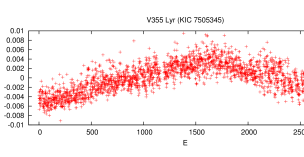
Figure 13.— Residual O$-$C diagram of V355 Lyr after we pre-whitened the data with the frequencies $kf_{\mathrm{B}}$, ($k=1,2,3,5$), and side peaks $f_{\mathrm{B}}\pm f_{\mathrm{L}}$.

The light curve of V355 Lyr (catalog ) in Fig. 4 suggests at least two modulation periods. The longer period amplitude change shows about four cycles during the four years observing span. It raises the possibility of an instrumental effect showing the Kepler year (372.5 d) (Bányai et al., 2013). Indeed, we found two strong peaks in the low frequency range of the spectrum which can be identified as $f_{\mathrm{K}}=0.00266$ and $2f_{\mathrm{K}}=0.00533$ d^-1. But other aspects contradict such an explanation. The Blazhko frequency turns up from the triplet structures and it is detectable directly as $f_{\mathrm{B}}=0.0322\pm 0.005$ d^-1. There is a detectable peak at $f=0.06154$ d^-1, (S/N=4.5) which can not be the harmonic $2f_{\mathrm{B}}$, because its difference from the exact harmonic (0.00147 d^-1) is twice of the Rayleigh frequency resolution ($\approx 0.0007$ d^-1). So we may identify it as a possible secondary modulation frequency ($f=f_{\mathrm{S}}$). If it is true, the two modulation frequencies are in a nearly 1:2 ratio, causing the observed beating phenomenon in the envelope curve.

At the same time the sub-harmonic $f_{\mathrm{B}}/2$ is also significant. A similar situation has been found for the first time by Sódor et al. (2011) in the case of the multiperodic Blazhko star CZ Lac (catalog ). Jurcsik et al. (2012) also detected the sub-harmonic of the Blazhko frequency for RZ Lyr (catalog ). As Sódor et al. (2011) discussed, we can also identify $f_{\mathrm{B}}/2$ as the primary modulation frequency. In that case instead of a sub-harmonic we would have a harmonic with much higher amplitude than the main modulation frequency. Moreover, the modulation curve would have a rather unusual shape. For these reasons we prefer the sub-harmonic identification.

As opposed to the above mentioned amplitude relations, the Fourier amplitude $A(f_{\mathrm{S}})$ is higher than $A(f_{\mathrm{B}})$ in the spectrum of the O$-$C curve. In other words, in FM $f_{\mathrm{S}}$ dominates, while in AM $f_{\mathrm{B}}$ is the dominant. Such an effect have never been detected before. Linear combination peaks at $f_{\mathrm{S}}\pm f_{\mathrm{B}}$ are also detectable. Additionally, the sub-harmonic of $f_{\mathrm{B}}$ can not be seen, but the sub-harmonic of $f_{\mathrm{S}}=0.03083$ d^-1 can be detected. One other significant peak is at $f^{(1)}=0.16316$ d^-1 (S/N=5.3). This frequency is located close to $5f_{\mathrm{B}}=0.16150$ d^-1 but the identification $f^{(1)}=5f_{\mathrm{B}}$ is ambiguous, because no other harmonics are detectable. The spectrum of the light curve also shows a marginal (S/N=2.4) peak at this position. We suspect that it might be a third modulation frequency. Pre-whitening the O$-$C curve with all the above mentioned frequencies we obtain the residual curve in Fig. 13. This residual shows a sudden period change at about $E\approx 1636$ (= BJD$\approx 2455778$) and a less pronounced one around $E\approx 2386$ (= BJD$\approx 2456133$). Nothing particular can be seen in the light curves around these dates.

Higher frequency range of the time series data is dominated by the main pulsation frequency, its harmonics, and their strong multiplet surroundings. Beyond the clear PD effect ($1.5f_{0}=3.155484$ d^-1; $P/P_{0}=1.495$) discussed by Szabó et al. (2010), the Fourier spectrum of the star shows evidences for the second radial overtone pulsation (see in Fig. 6). This feature was undetected by previous Kepler studies. The frequency $f_{2}=3.589528$ d^-1 ($P_{2}/P_{0}=0.588$) is surrounded by well separated side peaks.

3.2.8 V450 Lyr = KIC 7671081

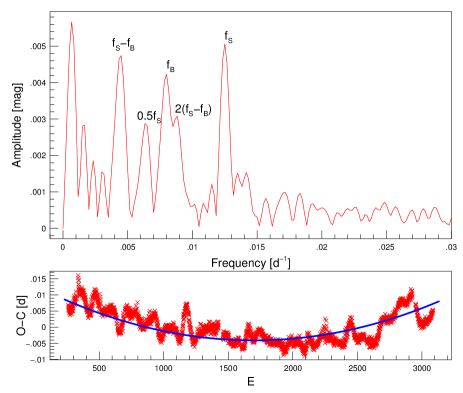
Figure 14.— Top: Zoom from the Fourier spectrum of the O$-$C diagram of V450 Lyr. Bottom: Residual O$-$C diagram after we pre-whitened the data with the above signed five frequencies. The best fitted parabola (continuous line) suggests a very fast period increase.

The shape of the maxima curve of V450 Lyr (catalog ) suggests a strong beating phenomenon between two modulation periods, however, similar features have also been seen in other stars (e.g. V355 Lyr and KIC 7257008) which proved to be instrumental effects. Accordingly, we carefully compared the frequencies determined in the spectra of the light curve and the O$-$C diagram. In the case of the light curve the largest low frequency peak $f_{\mathrm{K}}$ belongs to the Kepler year. The next one is the modulation frequency $f_{\mathrm{B}}=0.00813$ d^-1 ($A(f_{\mathrm{B}})$=6 mmag). Its harmonic $2f_{\mathrm{B}}$ is also detectable. The third largest amplitude peak is at the frequency $f_{\mathrm{S}}=0.01243$ d^-1. Low significance peaks are seen at the $f_{\mathrm{B}}+f_{\mathrm{S}}$ and $f_{\mathrm{S}}/2$ ($A(f_{\mathrm{B}}+f_{\mathrm{S}})\approx A(f_{\mathrm{S}}/2)\approx 2$ mmag).

A similar analysis on the spectrum of O$-$C diagram (see top panel in Fig. 14) results in two independent frequencies $f_{\mathrm{B}}$, $f_{\mathrm{S}}$ and some combinations of them ($f_{\mathrm{S}}-f_{\mathrm{B}}$, $f_{\mathrm{S}}-2f_{\mathrm{B}}$, $f_{\mathrm{S}}/2$). We can state now that $f_{\mathrm{S}}$ or $f_{\mathrm{S}}/2$ is a real secondary modulation frequency (See the discussion about the interpretation of the residual sub-harmonic in Sec. 3.2.7). When we subtract a fit with all the mentioned frequencies, the residual O$-$C diagram (bottom panel in Fig. 14) shows a combination of remained quasi-periodic signal and a parabolic shape indicating a strong period change. Fitting a quadratic function we found a fast period increase: $dP_{0}/dt=2.4\times 10^{-8}$ dd^-1, which can not be caused by stellar evolution. This phenomenon can be explained e.g. as a sign of a third longer period modulation or as a random walk caused by a quasi-periodic/chaotic modulation.

By investigating the fine structure of the Fourier spectrum between harmonics of the main pulsation frequency Molnár et al. (2014) recognized that V450 Lyr pulsates in the second radial overtone mode, as well (see also Fig. 6). If we identify the highest peak in this region at 3.33670 d^-1 with $f_{2}$, the period ratio is $P_{2}/P_{0}=0.594$, corresponding to canonical second overtone period ratio.

3.2.9 V353 Lyr = KIC 9001926

The AM of V353 Lyr displays alternating higher and lower amplitude Blazhko cycles (Fig. 4). The phenomenon reminds us the PD effect where the amplitudes of the consecutive pulsation cycles alternate. The effect suggests two modulation frequencies in a nearly 1:2 ratio. The low frequency region of the Fourier spectrum of the data is dominated by instrumental frequencies such as $f_{\mathrm{K}}$, $f_{\mathrm{K}}/2$, $f_{\mathrm{Q}}$ and $f_{\mathrm{Q}}/2$. If we remove these instrumental peaks, we find the two largest non-instrumental ones: $f_{\mathrm{B}}$=0.01386 d^-1 and $f^{(1)}$=0.00819 d^-1. We obtain 0.01394 and 0.00751 d^-1, respectively for these values from the spacings of the side peaks. The two frequencies are in the ratio of $\approx 1:2$ as we predicted. Since we detected sub-harmonic of the Blazhko frequency for several stars, $f^{(1)}$ could also be a sub-harmonic ($f^{(1)}=f_{\mathrm{B}}/2$) of $f_{\mathrm{B}}$.

The O$-$C diagram shows alternating maxima and minima again (Fig. 7). The Fourier spectrum of this curve is much simpler than the spectrum of the original light curve data. It contains $f_{\mathrm{B}}$=0.01395 d^-1 and its harmonic $2f_{\mathrm{B}}$, $f^{(1)}=f_{\mathrm{S}}=0.00761$ d^-1, and an additional discrete peak close to 0 representing a global long-term period change. Removing these three frequencies we obtain a residual spectrum which contains two significant peaks at 0.01462 d^-1 (S/N=11.8) and 0.02010 d^-1 (S/N=4). The most plausible identification of these peaks are $2f_{\mathrm{S}}$ and $f_{\mathrm{B}}+f_{\mathrm{S}}$, respectively. These frequencies, especially the linear combination, contradict the sub-harmonic scenario.

By removing all the mentioned frequencies we receive a parabolic shape diagram (which can be seen in Fig. 7). The period decrease calculating from the best fitted parabola is $-8.4\times 10^{-9}$ dd^-1 that can not be explained by an evolutionary effect. It shows hidden period(s) and/or chaotic variation.

To search for additional frequencies we pre-whitened the data with main frequency its harmonics and the largest 7-8 side peaks around the harmonics. We have found neither PD effect nor any higher order radial overtone modes (Fig. 6).

3.2.10 V366 Lyr = KIC 9578833

Figure 15.— The Fourier spectrum of the O$-$C diagram of V366 Lyr. Top panel: a possible identification of the peaks. Bottom panel: spectrum after we prewhitened with the four most significant frequencies above.

The maxima of the light curve show a beating like phenomenon (Fig. 4). Calculations from the multiplet structures and the determination of the significant low frequencies end in the same results. Beside the primary modulation frequency $f_{\mathrm{B}}$=0.0159 d^-1, two additional peaks can be detected at the frequencies $f^{(1)}=0.03415$ and $f^{(2)}=0.03175$ d^-1 with nearly equal amplitudes. The latter is the first harmonic of the Blazhko frequency, but the first one seems to belong to a secondary modulation frequency. Both of the primary ($kf_{0}\pm f_{\mathrm{B}}$) and secondary modulation side peaks ($kf_{0}\pm f_{\mathrm{S}}$) can be detected. The ratio between the two modulation frequencies is close to 1:2.

The O$-$C diagram (in Fig. 7) shows a typical beating signal. The spectrum is surprising (Fig. 15). Following our expectations it contains two close frequencies at $f_{\mathrm{B}}$=0.015932 d^-1 and $f^{(3)}=0.01823$ d^-1 which must be responsible for the beating phenomenon. Two other peaks are also visible. One of them is the harmonic of the primary modulation frequency ($2f_{\mathrm{B}}$), while the other is at the position of $f^{(1)}=f_{\mathrm{S}}=0.03414$ d^-1. In this framework we can identify $f^{(3)}=f_{\mathrm{S}}-f_{\mathrm{B}}$. Strangely enough, the amplitude of $f_{\mathrm{S}}$ is 1.55 times higher (1.7 vs 2.6 minutes) than that of $f_{\mathrm{B}}$. In other words, the roles of the primary and secondary Blazhko modulations are reversed. This is the second case for this new phenomenon (see also V355 Lyr in Sec. 3.2.7).

There is an alternate identification scenario for the detected frequencies. If we assume $f^{(3)}$ to be the genuine secondary modulation then the amplitudes would be in order: $A(f_{\mathrm{B}})=1.7>A(f_{\mathrm{S}})=1.1$ minutes, however, $f^{(1)}$ should be identified as $f_{\mathrm{B}}+f_{\mathrm{S}}$. In this case (i) the amplitude of the linear combination frequency would be higher than any of its elements. Moreover, since $f^{(1)}$ can be detected directly from the spectrum of the light curve, (ii) V366 Lyr (catalog ) would be the only case where a linear combination frequency is detectable instead of the secondary modulation frequency. For the above two (i and ii) reasons, we prefer the first scenario.

When we pre-whiten the O$-$C spectrum with the discussed four frequencies, additional significant peaks appear at some harmonics and linear combination frequencies, namely at $2f_{\mathrm{S}}$, $f_{\mathrm{S}}+f_{\mathrm{B}}$ and $2f_{\mathrm{B}}-kf_{\mathrm{S}}$ (bottom panel in Fig. 15). After subtracting all these significant frequencies, the residual O$-$C diagram shows no more structures.

On the basis of Q1-Q2 data no additional frequency pattern has been found for V366 Lyr (Benkő et al., 2010). The situation is changed when we take into account the Q1-Q16 time span. The highest peak between the harmonics is at the frequency $f^{(4)}=2.675799$ d^-1 (S/N=4.7, Fig. 6). The period ratio is $P^{(4)}/P_{0}$=0.71. Frequencies with similar period ratios were discovered in the CoRoT targets V1127 Aql (catalog ) and CoRoT 105288363 (catalog ), and Kepler stars V445 Lyr and V360 Lyr (catalog ) (Chadid et al., 2010; Guggenberger et al., 2012; Benkő et al., 2010). These frequencies are the dominant additional frequencies for only three stars: V1127 Aql, V360 Lyr and V366 Lyr.

The referred papers generally explain these frequencies as excitation of independent non-radial modes. As we showed in Benkő & Szabó (2014) all of these frequencies can be constructed by a linear combination as $f^{(4)}=2(f_{0}-f_{2})$. Here, in the case of V366 Lyr, we may identify the second overtone mode frequency with the marginal peak at $f_{2}=3.227711$ d^-1 (S/N=2.7). This formal mathematical description has its own strengths and weaknesses. As opposed to the non-radial explanation, it could be verified or denied by using existing radial hydrodynamic codes. It is hardly understandable, however, why linear combination $2(f_{0}-f_{2})$ is stronger than $f_{0}-f_{2}$.

3.2.11 V360 Lyr = KIC 9697825

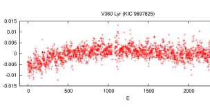
Figure 16.— Residual O$-$C diagram of V360 Lyr after we prewhitened the data with all significant frequencies.

The maxima of the light curve of V360 Lyr in Fig. 4 show a slight beating phenomenon. The Fourier spectrum contains rich multiplet structures around the harmonics of the main pulsation frequency. The largest side peaks indicate the following frequencies: $f_{\mathrm{B}}=0.01919$, $f^{(1)}=0.02374$, $f^{(2)}=0.02821$ and $f^{(3)}=0.04753$ d^-1. Two of them ($f_{\mathrm{B}}$ and $f^{(3)}$) can be detected directly, as well. If we assume $f^{(3)}$ to be a second independent modulation frequency ($f^{(3)}=f_{\mathrm{S}}$), the other two values can be expressed as $f^{(2)}=f_{\mathrm{S}}-f_{\mathrm{B}}$ and $f^{(1)}=f_{\mathrm{S}}/2$.

Beyond the above mentioned four frequencies, the Fourier spectrum of the O$-$C diagram shows two additional peaks at $2f_{\mathrm{B}}$ and $f_{\mathrm{S}}+f_{\mathrm{B}}$. We found again a Blazhko star which shows not only a secondary modulation but its half as well (see also discussion in Sec. 3.2.7). The ratio between the two modulation frequencies is 0.404 or 2:5. The residual curve of the O$-$C diagram (Fig. 16) shows a rather long period oscillation as a secular period change.

Two additional frequencies ($f_{1}=2.4875$ and $f^{\prime}=2.6395$ d^-1) of V360 Lyr were reported by Benkő et al. (2010) who explained $f_{1}$ with a possible first overtone mode and $f^{\prime}$ with an independent non-radial mode. As Szabó et al. (2010) have already mentioned $f^{\prime}$ could also be a member of a PD pattern around $f^{\prime}=1.5f_{0}$. When we analyze the Q1-Q16 data set the highest amplitude peak in this region is located at $f^{(4)}=2.678669$ d^-1 ($P^{(4)}/P_{0}=1.49$) which is a PD frequency without doubt.

Interpretation of the strongest additional peak at the frequency of $f^{(5)}=2.487740$ d^-1 is more problematic. The period ratio $P^{(5)}/P_{0}=0.721$ is far from the canonical value of the first radial overtone and fundamental modes (0.745). Such a ratio could be produced by a highly metal abundant RR Lyrae star (see e.g. fig. 8 in Chadid et al. 2010) but the metallicity of V360 Lyr is [Fe/H]=$-1.5\pm 0.35$ dex (N13). This difference might also be due to the resonance, which excites this mode in non-traditional way (Molnár et al., 2012). We suggested in Benkő & Szabó (2014) an other explanation: similarly to V366 Lyr (and V445 Lyr), this frequency could be a linear combination $2(f_{2}-f_{0})$, where $f_{2}=3.036015$ d^-1 is the frequency of the second radial overtone mode.

3.2.12 KIC 9973633

The history of the star is the same as that of KIC 7257008: the ASAS survey discovered it and its basic parameters were determined for the first time by N13. The Kepler data set of KIC 9973633 is relatively the most unfortunate in the analyzed sample. It has short time coverage (data exist from only Q10) and additional two quarters (Q11 and Q15) are missing (Fig. 4).

Although the triplet structures around the harmonics provide us the Blazhko frequency $f_{\mathrm{B}}$=0.01490 d^-1, we can not detect it directly in the low frequency range of the Fourier spectrum. Here the instrumental peak $f_{\mathrm{K}}$ dominates. When we remove it, we find two high amplitude peaks at $f_{\mathrm{K}}/2$ and $f^{(1)}=0.00411$ d${}^{-1}=f_{\mathrm{B}}-f_{\mathrm{Q}}$. After the next pre-whitening step we can see three peaks near the detection threshold at $f_{\mathrm{Q}}$, $f^{(2)}=0.03771$ d^-1 and $f^{(3)}=0.02701$ d^-1. It is easily recognizable that $f^{(3)}=f^{(2)}-f_{\mathrm{Q}}$. Which one is the real independent frequency: $f^{(2)}$ or $f^{(3)}$?

To investigate the question we analyzed the O$-$C diagram of KIC 9973633. The Fourier spectrum shows two highly significant peaks at $f_{\mathrm{B}}=0.01486$ d^-1 and $2f_{\mathrm{B}}=0.02972$ d^-1 (Fig. 8). By pre-whitening the data with these two frequencies we obtain a third one at 0.03675 d^-1. If we identify it with $f^{(3)}=f_{\mathrm{S}}$, we are in a similar situation as in the case of V360 Lyr (Sec. 3.2.11): we have two modulation frequencies with the ratio of 2:5. The residual of the O$-$C diagram does not show any structures: it is a constant line with some scatter.

3.2.13 V838 Cyg = KIC 10789273

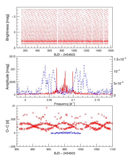
Figure 17.— Analysis of V838 Cyg (catalog ). The top panel shows the synthetic light curve prepared by using the Fourier parameters of the observed data without assuming any modulations and sampled on the Kepler data points (cf. Fig. 4). Middle panel: Fourier spectra of the observed (red continuous line) and synthetic (blue dashed line) time series around the pulsation frequency after the data were pre-whitened with the main frequency. The left and right hand side magnitude scales belong to the observed and synthetic spectra, respectively. Bottom panel: Part of the O$-$C diagrams for LC data (red crosses) and SC observations (blue dots).

The extremely low amplitude Blazhko modulation of V838 Cyg was discovered by N13. The light curve in Fig. 4 shows wavy maxima and minima, however, this is structure produced by interference of the sampling and the pulsation frequencies and it does not indicate any AM. It is a virtual modulation and not a real one. It means that we need more careful investigations to decide whether V838 Cyg is modulated or not. Clear triplets around the main pulsation frequency and its harmonics in the Fourier spectrum suggest a modulation phenomenon with the frequency of $f_{\mathrm{B}}=0.01681$ d^-1. It follows that the period is $P_{\mathrm{B}}=59.5$ d which roughly agrees with the dominant modulation period value (54-55 d) found by N13.

V838 Cyg was observed in SC mode in only one quarter in Q10. We processed these pixel data in the same way as we have done for LC data. The obtained SC light curve does not show virtual modulation like LC data, but shows a small amplitude change. This variation is, however, hard to distinguish from possible instrumental trends. To test the presence of the modulation we made synthetic data. We prepared an artificial time series $m_{\mathrm{syn}}(t)$ using the Fourier parameters of the observed data such as $f_{0}$, $A_{k}$ and $\varphi_{k}$, where $A_{k}$ and $\varphi_{k}$ mean the amplitude and phase values of the $k$th harmonics ($k=1,2,\dots,11$) i.e. without modulation side peaks:

$$m_{\mathrm{syn}}(t)=\sum_{k=1}^{11}A_{k}\sin(2\pi f_{0}t+\varphi_{k}).$$

The synthetic data were sampled at the observed time stamps $t$ (top panel in Fig. 17).

The spectra of the observed and synthetic data have systematic differences (see middle panel in Fig. 17). (i) In the case of synthetic data the side peaks have $\approx 80$ times smaller amplitudes than the observed ones (0.012 mmag vs. 1 mmag). (ii) The position of the side frequencies are different. (iii) The structures of these side patterns are also different: the observed data show simple clear triplet, while the synthetic data produce complicated multiplets. To summarize, we confirmed the AM with an independent method. Since the amplitude of the modulation is very small, we could not detect $f_{\mathrm{B}}$ directly from the low frequency range of the Fourier spectrum. This part of the spectrum is dominated by instrumental frequencies ($f_{\mathrm{K}}$, $f_{\mathrm{L}}$, where $P_{\mathrm{L}}=1/f_{\mathrm{L}}$ indicates the total length of the observation: $\sim 4$ years). N13 mentioned possible multiple modulations. After pre-whitening the data with the side frequencies $kf_{0}\pm f_{\mathrm{B}}$ only instrumental side peaks ($kf_{0}\pm f_{\mathrm{K}}$ $kf_{0}\pm f_{\mathrm{L}}$) remain significant around the harmonics.

We can not construct the O$-$C diagram the traditional way because the sparse continuous sampling with the relatively short pulsation period and the interpolation errors produce systematic undulations (in the bottom panel in Fig. 17). Due to the long Blazhko period, the analysis of SC data does not help too much. The sensitive method used by N13 resulted in 0.001 radian phase variation in $\varphi_{1}$ which predicts about $5\times 10^{-4}\approx 40$ s O$-$C variation. It is about our detection limit: the standard deviation of O$-$C for SC data is $\approx 2\times 10^{-4}$. Our analysis supports the phase modulation reported by the discovery paper.

We also found additional frequency patterns for the first time in this star. After we subtracted the significant harmonics of the pulsation frequency and triplets around them, the following additional frequencies can be detected between $f_{0}$ and $2f_{0}$: $f_{2}=3.509142$ d^-1, $1.5f_{0}=3.113906$ d^-1 (PD) and $3f_{0}-f_{2}=2.737256$ d^-1, respectively (see Fig. 6).

3.2.14 KIC 11125706

Though KIC 11125706 shows the second lowest amplitude AM in our sample, its long pulsation period allows us to detect it without any problems. The asymmetric triplet structures around the pulsation frequency and its harmonics provide $f_{\mathrm{B}}$. Direct detection of this frequency has failed. The low frequency range of the Fourier spectrum is dominated by instrumental peaks.

Contrary to this, the Fourier spectrum of the O$-$C diagram (Fig. 8) contains a very significant (S/N=37.8) peak at $f_{\mathrm{B}}$. Pre-whitening with this frequency, a lower amplitude, but clearly detectable ($A(f^{(1)})=1.9\times 10^{-4}$ d, S/N=$6.4$) peak can be seen at $f^{(1)}=0.01698$ d^-1. Is it a real secondary modulation frequency or results from the sampling? We generated synthetic O$-$C data using the Fourier parameters of the primary Blazhko period and added Gaussian noise to it. The synthetic diagram was sampled exactly at the same points as the observed one. The Fourier spectrum of the artificial O$-$C curve contains only the $f_{\mathrm{B}}$ and it does not show any other significant peaks. Thus we ruled out an instrumental origin of this frequency. Now, we tend to identify $f^{(1)}=f_{\mathrm{S}}$. In this case the two modulation frequencies are in a ratio of nearly 3:2. The quadratic fit of the residual O$-$C gives a slight period increase: $dP_{0}/dt=4.4\times 10^{-10}\pm 1.1\times 10^{-10}$ dd^-1.

Returning to the light curve analysis we do not find any significant frequencies around $f_{\mathrm{S}}$ and no side peaks detected which could belong to this frequency. These facts mean that the AM of $f_{\mathrm{S}}$ is below of our detection limit. Furthermore, no additional peak patterns have been found between harmonics (Fig. 6).

3.2.15 V1104 Cyg = KIC 12155928

Beyond V2178 Cyg, V1104 Cyg was also the subject of the case study of N13. We can add only few things to this study. We derived the Blazhko cycle based on a longer time span. The frequency of the Blazhko modulation $f_{\mathrm{B}}$ is highly significant both in the Fourier spectrum of the light curve and that of the O$-$C diagram. The latter spectrum also includes the harmonic $2f_{\mathrm{B}}$ (Fig. 8) indicating non-sinusoidal behavior of the FM. The O$-$C residual does not indicate any period changes during the Kepler time-scale. Our analysis resulted in neither secondary modulation nor additional frequencies between harmonics (Fig. 6).

4. Conclusions

The main goal of this paper was to investigate the long time-scale behavior of the Blazhko effect among the Kepler RR Lyrae stars. To provide the best input for the analysis we prepared time series from the pixel photometric data with our own tailor-made aperture. These light curves include the total flux of the stars for only 9 cases while some portion of the flux of 6 RR Lyrae stars was lost using even in the largest possible aperture. Nevertheless, our data set comprises the longest continuous, most precise observations of Blazhko RR Lyrae stars ever published. These data will be unprecedented for years to come.

Since the Blazhko effect manifests itself in simultaneous AM and FM we analyzed both phenomena and compared the results of the separated analyses. This approach reduces the influence of the instrumental effects.

We detected single Blazhko period for three stars: V783 Cyg, V838 Cyg and V1104 Cyg. Since V838 Cyg shows the smallest amplitude modulation both in AM and FM, we could not confirmed its multiperiodicity which was suspected by N13.

Twelve stars in our sample show evidences for multiperiodic modulation. In eight cases we could determine two significant Blazhko periods, while for four additional cases (V2178 Cyg, V808 Cyg, V354 Lyr and KIC 7257008) we could establish the presence of a possible long secondary period. It does not mean, however, that we could described the total variations with these one or two periods completely. The residual curves show significant structures (see e.g. V2178 Cyg, V808 Cyg, V450 Lyr) after subtracting the best fitted light/O$-$C curves. For the 2-3 stars with the shortest Blazhko periods we have a chance to carrying out a dynamical analysis. In this work we mentioned the preliminary result from the cycle-to-cyle variation of V783 Cyg modulation (Plachy et al. in prep.) which hints for its chaotic nature.

The latest and most complete compilation of the Galactic Blazhko RR Lyrae stars (Skarka, 2013) consists only 8 multiperiodic cases among 242 known field Blazhko RR Lyrae stars (3.3%). More recently Skarka (2014) studied a more homogeneous 321 elements sample from the ASAS and SuperWASP surveys. He found the ratio of the multiperiodic and irregularly modulated stars to be 12%. In this work we surprisingly found that most of the Kepler Blazhko stars – 12 from 15 (80%) – belongs to the multiperiodic group. In other words: the Blazhko effect predominantly manifests as a multiperiodic phenomenon instead of a mono-periodic and regular one. Here we briefly summarize the main characteristics of the multiperiodic modulations.

• Up to now the known smaller amplitude (secondary) modulation periods were generally longer than the primary ones. The only exception is RZ Lyr (Jurcsik et al., 2012). Here we showed five further examples (V355 Lyr, V450 Lyr, V366 Lyr, V360 Lyr and KIC 9973633) for shorter secondary periods.

• What is more, the definition of the primary and secondary modulations proved to be relative. In three cases (for V450 Lyr, V366 Lyr and V355 Lyr) the relative strength of the primary modulations is weaker in FM than in AM.

• The linear combination of the modulation frequencies can generally be detected that indicates the nonlinear coupling between the modes. Sub-harmonic frequencies ($f_{\mathrm{B}}/2$ and/or $f_{\mathrm{S}}/2$) were detected for numerous cases (KIC 7257008, V355 Lyr, V450 Lyr, V360 Lyr). In the majority of the cases the two modulation periods are in a ratio of small integer numbers: 1:2 for V353 Lyr; 2:1 for V366 Lyr and V355 Lyr; (3:2 for V2178 Cyg); 2:3 for KIC 11125706; 5:2 for KIC 9973633 and V360 Lyr. (Here the ratios of the primary AM period vs. secondary one are indicated.)

As a by-product of the analysis we report here for the first time additional frequency structures for V808 Cyg, V355 Lyr and V838 Cyg. For all three cases we detected the second radial overtone mode $f_{2}$.

The former studies of CoRoT and Kepler Blazhko data found unidentified frequencies for numerous stars. These frequencies were explained by non-radial mode excitation. Here we showed that almost all of such frequencies can also be produced by linear combinations of radial modes. The only case where we could not find a proper linear combination is the highest amplitude additional frequency of V354 Lyr.

The amplitudes of these frequencies point to rather the non-radial mode scenario. These non-radial modes may be excited by resonances at the locations of the linear combination of the radial modes (Van Hoolst et al., 1998). In other words, these frequencies are linear combinations from mathematical point of view only, and physically they are frequencies of independent (non-radial) modes.

References

- Bányai et al. (2013) Bányai, E., Kiss, L. L., Bedding, T., et al. 2013, MNRAS, 436, 1576
- Benkő et al. (2010) Benkő, J.M., Kolenberg, K., Szabó, R., et al. 2010, MNRAS, 409, 1585
- Benkő, Szabó & Paparó (2011) Benkő, J.M., Szabó, R. & Paparó, M. 2011, MNRAS, 417, 974
- Benkő & Szabó (2014) Benkő, J.M. & Szabó, R. 2014, in Precision Asteroseismology, Guzik, J.A., Chaplin, W.J., Handler, G., Pigulski, A., eds. IAU Symp. 301, p. 383
- Blazhko (1907) Blazhko S. N. 1907, Astron. Nachr., 175, 325
- Breger et al. (1999) Breger, M., Handler, G., Garrido, R. et al. 1999, A&A, 349, 225
- Buchler & Kolláth (2011) Buchler, J.R. & Kolláth, Z. 2011, ApJ, 731, 24
- Chadid et al. (2010) Chadid M., Benkő J. M., Szabó R. et al. 2010, A&A, 510, A39
- Cross (1991) Cross, J. 1991, J. AAVSO 20, 214
- Fanelli et al. (2011) Fanelli, M.N., Jenkins, J.M., Bryson, S. et al. 2011, Kepler Data Processing Handbook, NASA Ames Research Center, Moffett Field
- Guggenberger et al. (2012) Guggenberger, E., Kolenberg, K., Nemec, J.M., et al. 2012, MNRAS, 424, 649
- Jenkins et al. (2010a) Jenkins J. M., Caldwell D. A., Chandrasekaran H. et al. 2010a, ApJ, 713, L87
- Jenkins et al. (2010b) Jenkins J. M., Caldwell D. A., Chandrasekaran H. et al. 2010b, ApJ, 713, L120
- Jenkins et al. (2013) Jenkins J. M., Caldwell D. A., Barclay Th. et al. 2013, Kepler Data Characteristics Handbook, NASA Ames Research Center, Moffett Field
- Jurcsik et al. (2012) Jurcsik J., Sódor Á., Hajdu G. et al., 2012, MNRAS, 427, 1517
- Koch et al. (2010) Koch D. G., Borucki W. J., Basri G., et al. 2010, ApJ, 713, L79
- Kolenberg (2012) Kolenberg, K. 2012, J. AAVSO, 40, 481
- Kolenberg et al. (2010) Kolenberg K., Szabó R., Kurtz D. W. et al. 2010, ApJ, 713, L198
- Kolenberg et al. (2011) Kolenberg K., Bryson, S., Szabó R. et al. 2011, MNRAS, 411, 878
- Kolláth (1990) Kolláth Z., 1990, Occ. Tech. Notes. Konkoly Obs. No 1.
- Kolláth et al. (2002) Kolláth Z., Buchler, J.R., Szabó, R. & Csubry, Z. 2002, A&A, 385, 932
- Kolláth, Molnár & Szabó (2011) Kolláth Z., Molnár, L. & Szabó, R. 2011, MNRAS, 414, 1111
- Kovács (2009) Kovács G., 2009, in Guzik J.A., Bradley P., eds., AIP Conf.Proc. 1170, Stellar Pulsation: Challanges for Theory and Observation, p. 261
- Lenz & Breger (2005) Lenz P. & Breger M. 2005, CoAst, 146, 53
- Molnár, Kolláth & Szabó (2012) Molnár, L., Kolláth, Z. & Szabó, R. 2012, MNRAS, 424, 31
- Molnár et al. (2012) Molnár, L., Kolláth, Z., Szabó, R., et al. 2012, ApJ, 757, L13
- Molnár et al. (2014) Molnár, L., Benkő, J.M., Szabó, R. & Kolláth, Z. 2014, in Precision Asteroseismology, Guzik, J.A., Chaplin, W.J., Handler, G., Pigulski, A., eds. IAU Symp. 301, p. 459
- Nemec et al. (2011) Nemec, J.M., Smolec, R., Benkő, J.M., et al. 2011, MNRAS, 417, 1022
- Nemec et al. (2013) Nemec, J.M., Cohen, J.G., Ripepi, V., et al. 2013, ApJ, 773, id.181 N13
- Pojmanski, G. (1997) Pojmanski, G. 1997, AcA, 47, 467
- Pojmanski, G. (2002) Pojmanski, G. 2002, AcA, 52, 397
- Reegen (2007) Reegen P., 2007, A&A, 467, 1353
- Skarka (2013) Skarka M. 2013, A&A, 549, A101
- Skarka (2014) Skarka M. 2014, A&A, 562, A90
- Smolec et al. (2011) Smolec, R., Moskalik, P., Kolenberg, K., et al. 2011, MNRAS, 414, 2950
- Sódor et al. (2011) Sódor Á., Jurcsik J., Szeidl, B. et al. 2011, MNRAS, 411, 1585
- Sterken (2005) Sterken, C. 2005, in The Light-Time Effect in Astrophysics, C. Sterken, ed., ASP Conf. Ser. 335, p. 3
- Stothers (2006) Stothers R. B. 2006, ApJ, 653, 73
- Szabó et al. (2010) Szabó R., Kolláth, Z., Molnár L., et al. 2010, MNRAS, 409, 1244
- Szabó et al. (2014) Szabó R., Benkő, J.M., Paparó M., et al. 2014, A&A, (submitted)
- Van Cleve et al. (2009) Van Cleve, J., Caldwell, D., Thompson, R., et al. 2009, Kepler Instrumental Handbook, NASA Ames Research Center, Moffett Field
- Van Hoolst et al. (1998) Van Hoolst, T., Dziembowski, W.A. & Kawaler, S.D. 1998, MNRAS, 297, 536