Chaos in Lifshitz Spacetimes

Xiaojian Bai¹, Junde Chen², Bum-Hoon Lee¹, and Taeyoon Moon³

¹Center for Quantum Spacetime, Sogang University, Seoul, Korea

²Department of Physics, Shandong University, Jinan, China

³Institute of Basic Sciences and School of Computer Aided Science,

Inje University, Gimhae, Korea

baixj@sogang.ac.kr, chunte@mail.sdu.edu.cn, bhl@sogang.ac.kr, tymoon@inje.ac.kr

We investigate the chaotic behavior of a circular test string in the Lifshitz spacetimes considering the critical exponent $z$ as an external control parameter. It is demonstrated that two primary tools to observe chaos in this system are Poincaré section and Lyapunov exponent. Finally, the numerical result shows that if $z=1$, the string dynamics is regular, while in a case slightly larger than $z=1$, the dynamics can be irregular and chaotic.

1 Introduction

The AdS/CFT correspondence [1, 2, 3] is a powerful tool to describe strongly correlated system in terms of weakly coupled gravitational dynamics, and vice versa. Recently, it has been conjectured, on the analogy of the relativistic AdS/CFT correspondence, the existence of a similar holographic dual description in condensed matter physics [4, 5], which corresponds to non-relativistic system without Lorentz invariance. In such a theory, scaling transformation of time and space take the form anisotropically

$$t\to\lambda^{z}t,~{}~{}~{}~{}~{}x\to\lambda x,$$ (1.1)

where $z$ is a dynamical critical exponent, revealing the anisotropy between space and time whenever $z\neq 1$. It is well-known that the so called Lifshtiz metric with scaling symmetry (1.1) in $D$ dimensions provides a geometric description of Lifshitz spacetimes [6, 7, 8]:

$$ds^{2}=\ell^{2}\left(-r^{2z}dt^{2}+\frac{dr^{2}}{r^{2}}+r^{2}dx_{i}^{2}\right),$$ (1.2)

where $i=2,3,\cdots,D-1$. However, it was shown in the literature [4, 8, 9] that the Lifshitz geometry ($z\neq 1$) has a problem of null curvature singularity by calculating the tidal forces between infalling geodesics. More precisely, in Ref. [10] the authors demonstrated that Lifshitz solutions are unstable by showing that the test strings become infinitely excited when crossing the singularity. Very recently, it was suggested in Ref.[11] that Lifshitz singularity problem can be resolved by recognizing that string propagation is modified enough to avoid singular tidal forces when considering nontrivial matter contents, which corresponds to stress-energy sources.

In this paper, we investigate this kind of the Lifshitz instability which is present whenever $z\neq 1$, from an alternative point of view, i.e., chaos. It is demonstrated that dynamical instability of a nonlinear system, which is described by a nonlinearity of the equations of motion in most cases, could be provided chaoticity of the system. It is well known that a test particle motion is completely regular, that is, integrable (non-chaotic) in the generic Kerr-Newmann background [13] and the particle geodesic equation can be analytically solved in higher dimensional spherically symmetric spacetimes [14]. On the contrary of the case of the particle geodesic, it was shown that the motion of test strings can exhibit chaotic behavior in spherically symmetric black hole [15], AdS soliton [16], and AdS${}_{5}\times$ T^1,1 [17] background. More interestingly, in Ref. [18] the chaotic behavior of the classical string was studied in the context of the gauge/gravity correspondence.

Along this line of research containing the test string, we intend to investigate the chaotic behavior of the circular test string moving in the Lifshitz spacetimes by thinking of the critical exponent $z$ as an external control parameter. A key motivation for introducing the control parameter $z$ is to examine the relation between space time anisotropy and chaos. Our quantitative approaches to identifying and measuring chaos in this system include two numerical techniques; one is to check for the breaking of the KAM (Kolmogorov-Arnold-Moser) tori [19] through the numerical computation of the Poincaré sections [20] and the other is to calculate the maximum Lyapunov exponent $\lambda$, in which the defining signature of chaos takes the positive $\lambda$. Using both the poincaré sections and Lyapunov exponent in the Lifshitz spacetimes, we show explicitly that if $z=1$, the string dynamics is regular, while in the case slightly off $z=1$, the dynamics can be irregular and chaotic.

2 Instability of the Lifshitz spacetimes

Let us begin by introducing the following Lifshitz metric [21]:

$$ds^{2}=-\frac{r^{2z-2}}{\ell^{2z-2}}f(r)dt^{2}+\frac{1}{f(r)}dr^{2}+r^{2}d\theta^{2}+r^{2}\sin^{2}\theta d\varphi^{2},$$ (2.1)

where $z$ denotes the critical exponent, $\ell$ is the curvature radius of Lifshitz spacetimes, and metric function $f(r)$ is given by

$$f(r)=\frac{1}{z^{2}}+\frac{r^{2}}{\ell^{2}}.$$ (2.2)

We note that the Lifshitz metric (2.1) reduces simply to AdS spacetimes when $z=1$. However, if $z\neq 1$, as was shown in [10], the tidal forces in the Lifshitz geometry diverge as $(z-1)/r^{2z}$, which implies that there is a curvature singularity at $r=0$. To see this more concretely, we consider a radial timelike geodesic with the normalization $U_{\mu}U^{\mu}=-1$, where tangent vector $U^{\mu}$ is given by $U^{\mu}=(\dot{t},\dot{r},0,0)$. Here the dot ‘$\cdot$’ denotes the differentiation with respect to the proper time $\tau$. Now we introduce a parallel orthonormal frame field along the geodesic

$$e_{(0)}^{~{}\mu} = \frac{E}{fr^{2(z-1)}}\left(\frac{\partial}{\partial t}\right)^{\mu}-\frac{E}{r^{z-1}}\sqrt{\frac{1}{\ell^{2z-2}}-\frac{fr^{2(z-1)}}{E^{2}}}\left(\frac{\partial}{\partial r}\right)^{\mu},$$

$$e_{(1)}^{~{}\mu} = \frac{E}{fr^{2(z-1)}}\sqrt{1-\frac{fr^{2(z-1)}\ell^{2(z-1)}}{E^{2}}}\left(\frac{\partial}{\partial t}\right)^{\mu}-\frac{E}{r^{z-1}\ell^{z-1}}\left(\frac{\partial}{\partial r}\right)^{\mu},$$

$$e_{(2)}^{~{}\mu} = \frac{1}{r}\left(\frac{\partial}{\partial\theta}\right)^{\mu},~{}~{}~{}~{}e_{(3)}^{~{}\mu}~{}=~{}\frac{1}{r\sin\theta}\left(\frac{\partial}{\partial\varphi}\right)^{\mu},$$

where Greek indices denote spacetime coordinates $(t,r,\theta,\varphi)$ and indices enclosed in parentheses describe the flat tangent space in which the orthonormal frame is defined. In the above expressions, the conserved energy $E$ can be written by $E=\dot{t}fr^{2(z-1)}$. It turns out that in this orthonormal frame, we have the non-vanishing components of the Riemann tensor as follows:

$$R_{(0)(1)(0)(1)}=\frac{(z-1)(z-2)}{z^{2}r^{2}}+\frac{z^{2}}{\ell^{2}},~{}~{}~{}~{}R_{(0)(2)(0)(2)}=R_{(0)(3)(0)(3)}=\frac{E^{2}\ell^{2(1-z)}(z-1)}{r^{2z}}+\frac{1}{\ell^{2}}$$ (2.3)

$$R_{(2)(3)(2)(3)}=\frac{z^{2}-1}{z^{2}r^{2}}-\frac{1}{\ell^{2}},~{}~{}~{}~{}R_{(1)(2)(1)(2)}=R_{(1)(3)(1)(3)}=\frac{E^{2}\ell^{2(1-z)}(z-1)}{r^{2z}}-\frac{z-1}{z^{2}r^{2}}-\frac{z}{\ell^{2}}$$ (2.4)

$$R_{(0)(2)(1)(2)}=R_{(0)(3)(1)(3)}=\frac{E^{2}\ell^{2(1-z)}(z-1)}{r^{2z}}\sqrt{1-\frac{\ell^{2z-4}r^{2(z-1)}(\ell^{2}+z^{2}r^{2})}{E^{2}z^{2}}},$$ (2.5)

where the Riemann tensor in the orthonormal frame is defined by $R_{(a)(b)(c)(d)}=R_{\mu\nu\rho\sigma}e_{(a)}^{~{}\mu}e_{(b)}^{~{}\nu}e_{(c)}^{~{}\rho}e_{(d)}^{~{}\sigma}$. The resulting components of the Riemann tensor show that whenever $z\neq 1$, the Lifshitz geometry is unstable due to the divergence as $(z-1)/r^{2z}$ or $(z-1)/r^{2}$ in the limit $r\to 0$. Most of all, it is demonstrated in the literature [10] that Lifshitz solutions can be unstable by showing that the test strings become infinitely excited when crossing the singularity. In the present paper, however, we study the nature of this instability in an alternative point of view, i.e., chaos. It is of importance to note that the presence of chaos in a given spacetimes would be a geometrical criterion of local instability. On the other hand, the chaotic behavior of a test object moving in the system can be a key observation of instability when examining if the system is stable or not. For this purpose, we investigate the chaotic behavior of a circular test string moving near $r=0$ in the Lifshitz spacetimes by considering the critical exponent $z$ as an external control parameter. Before proceeding further, we first introduce a circular string moving in the Lifshitz spacetimes in the next section.

3 Circular string in the Lifshitz spacetimes

In order to investigate the behavior of a test string in the Lifshitz spacetimes, let us first consider the Nambu-Goto action

$$S=-T\int~{}d\tau d\sigma\sqrt{-{\rm det}[h_{ab}]}~{}~{}{\rm with}~{}~{}h_{ab}=g_{\mu\nu}\partial_{a}X^{\mu}\partial_{b}X^{\nu},$$ (3.1)

where $T$ is the string tension, $h_{ab}$ is the induced metric on the worldsheet, $g_{\mu\nu}$ is the spacetime metric, and $X^{\mu}=X^{\mu}(\tau,\sigma)$ are the spacetime coordinates of the string. The index $a$ and $b$ in the action (3.1) run over values $(\tau,\sigma)$. Varying the action (3.1) with respect to $X^{\mu}$ leads to the string equations of motion

$$\ddot{X}^{\mu}-X^{\prime\prime\mu}+\Gamma^{\mu}_{\rho\sigma}(\dot{X}^{\rho}\dot{X}^{\sigma}-X^{\prime\rho}X^{\prime\sigma})=0,$$ (3.2)

where the dot ‘$\cdot$’ and prime ‘$\prime$’ denote the differentiation with respect to the string world sheet coordinates $\tau$ and $\sigma$, respectively. On the other hand, Weyl invariance and reparametrization invariance allow us to choose the conformal gauge $h_{ab}=\Omega^{2}\eta_{ab}$, where $\eta_{ab}$ is locally flat and $\Omega$ is a scalar function of the worldsheet coordinates $(\tau,\sigma)$. It turns out that in this gauge, the corresponding conditions are given by $h_{\tau\sigma}=0$ and $h_{\tau\tau}+h_{\sigma\sigma}=0$, which lead to the constraints

$$g_{\mu\nu}\dot{X}^{\mu}X^{\prime\nu}=g_{\mu\nu}(\dot{X}^{\mu}\dot{X}^{\nu}+X^{\prime\mu}X^{\prime\nu})=0.$$ (3.3)

Now we consider the circular string, which is obtained by the ansatz:

$$t=t(\tau),~{}~{}~{}r=r(\tau),~{}~{}~{}\theta=\theta(\tau),~{}~{}~{}\varphi=\sigma.$$ (3.4)

With the circular string ansatz (3.4), the equations of motion (3.2) and constraints (3.3) in the Lifshitz background (2.1) yield

$$\dot{t}~{}=~{}\frac{E}{fr^{2(z-1)}}$$

$$\ddot{r}~{}=~{}\frac{1-z}{r}\dot{r}^{2}+\Big{(}(2-z)rf-\frac{r^{2}}{2}f^{\prime}\Big{)}\dot{\theta}^{2}-(zrf+\frac{r^{2}}{2}f^{\prime})\sin^{2}\theta=0$$ (3.5)

$$\ddot{\theta}=-\frac{2}{r}\dot{r}\dot{\theta}-\sin\theta\cos\theta$$ (3.6)

$$\ell^{2z-2}r^{2z-2}\Big{(}\dot{r}^{2}+fr^{2}(\dot{\theta}^{2}+\sin^{2}\theta)\Big{)}=E^{2}$$ (3.7)

Note that the constraint (3.7) is the same with the one obtained from the Hamiltonian constraint $H=0$ for the following Hamiltonian

$$H=\frac{1}{2}fP_{r}^{2}+\frac{1}{2r^{2}}P_{\theta}^{2}-\frac{\ell^{2-2z}r^{2-2z}}{2f}E^{2}+\frac{1}{2}r^{2}\sin^{2}\theta,$$ (3.8)

where $P_{r}=\dot{r}/f$ and $P_{\theta}=r^{2}\dot{\theta}$.

We mention that it is a formidable task to solve the above equations (3.5)$\sim$(3.7) analytically, because they are non-integrable. Thus we will analyze the equations numerically in the next section. We remind that our primary purpose is to investigate the chaoticity of a given non-integrable system in such a way that we treat the critical exponent $z$ as an external control parameter and we will use a couple of quantitative approaches to identifying and measuring chaos; Poincaré sections and Lyapunov exponent.

4 Numerical results

Poincaré sections

,
,
,

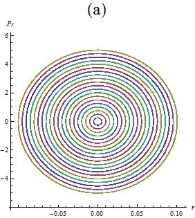
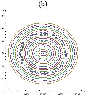
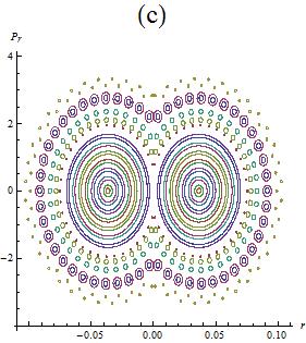
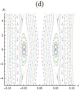
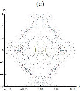
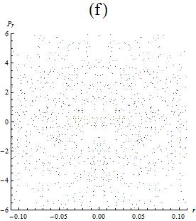
Figure 1: The Poincaré sections for $E=50$, $\ell=1$ in isotropic (a) and anisotropic (b)$\sim$(f) cases. Fig. 1(a) corresponds to $z=1$ and (b) to 1.00008, (c) 1.001, (d) 1.025, (e) 1.03, (f) 1.045. The figure 1(a) consists of the sets of KAM tori only (non chaotic), while for the figures (b)$\sim$(e) the KAM tori break up and it is eventually shown the Cantor sets in Fig. 1(f).

In order to investigate whether the string’s particular orbit can show the chaotic behavior or not, we first check for the breaking of the KAM tori which is indicative of chaos for a given system by numerical computation of the Poincaré sections in the phase space ($r,P_{r}$). On the other hand, if Poincaré sections consist of continuous closed lines without revealing an essentially random series of dots, the system is not chaotic. It is of importance to note that since our main interest is to explore the connection between chaotic behavior and spacetime anisotropy ($z\neq 1$), the critical exponent $z$ in our numerical analysis plays a central role of an external control parameter. To this end, we shall focus on the cases $z=1$ (isotropic) and slightly larger (anisotropic) than $z=1$. Note that for fixed $E$ and $\ell$, we set initial values of ($\dot{r},\theta$) at $\tau=0$ as $\dot{r}(0)=0$ and $\theta(0)=0$. The initial value $\dot{\theta}(0)$ can be determined by the constraint equation (3.7) when varying a value of $r(0)$. In other words, the string trajectories for various initial conditions can be obtained from integrating equations (3.5) and (3.6). As a result, the Poincaré sections for different initial conditions and fixed $E=50,~{}\ell=1$ are presented in Fig. 1(a) and (b)$\sim$ (f), illustrated with $z=1$ and $z\neq 1$, respectively. In these figures different colors correspond to different values of $r(0)$.

A few explanations for the figure $1$ are in order. First, Fig. 1(a) consists of KAM tori only, which implies that the corresponding motion is non chaotic. Whereas, Fig. 1(b) being slightly off $z=1$ shows that some KAM tori break up into discrete segments and new sets of smaller tori emerge. Second, being a few more off the point $z=1$ (see Fig. 1(c)), it seems that the largest KAM torus in Fig. 1(b) is decomposed into two smaller tori and the total number of tori is much more than that in Fig. 1(b). The figure 1(d) indicates that most of the tori break up and eventually scatter. In the last, there exist the sets of sparse points in almost whole (Fig. 1(e)) and full ranges (Fig. 1(f)) corresponding to the Cantor sets (cantori).

Lyapunov exponent

A more quantitative method one uses to investigate chaos is to calculate the largest Lyapunov exponent in a given system. If we consider the growth rate between two initially nearby trajectories, the largest Lyapunov exponent $\lambda$ is defined as

$$\lambda(t)=\frac{1}{t}\ln\Big{[}\frac{dX(t)}{dX(0)}\Big{]},$$ (4.1)

where $dX$ is the difference between two points in phase space, which corresponds, more precisely, to the Cartesian distance between $(r,\dot{r},\theta,\dot{\theta})$ and $(\tilde{r},{\dot{\tilde{r}}},\tilde{\theta},{\dot{\tilde{\theta}}})$ of two nearby phase space trajectories. We note that in a chaotic system, the growth rate in logarithm in Eq.(4.1) will be exponential in time with a positive constant $\lambda$, while for a regular system the rate is expected to be linear or power law growth in time, which implies that the Largest Lyapunov exponent $\lambda$ goes to zero in the limit $t\to\infty$. Thus, it is obvious that our goal in this section is to observe the positive Lyapunov exponent, which may be taken as the defining signature of chaos.

On the other hand, our numerical analysis begins with a set of initial values for $z=1.01$, $E=20,~{}\ell=1,$ which is given as follows: $r(0)=1/2,~{}\dot{r}(0)=0,~{}\theta(0)=0$, and $~{}\dot{\theta}(0)=36.31,$ where $\dot{\theta}(0)$ is determined by the constraint equation (3.7). We also consider an initial tiny separation as $\delta_{0}=10^{-3}$ for a nearby point $r(0)+\delta_{0}$. With these initial values, we try to compute the Lyapunov exponent [Eq.(4.1)] following the algorithm provided by Sprott [22, 23]. As a consequence, we present in figure 2 the result of estimating the largest Lyapunov exponent with a convergent positive value, which implies that the motion can be chaotic when $z\neq 1$. On the contrary, it is checked that the Lyapunov exponent becomes almost zero ($\sim 10^{-3}$) for $z=1$, which corresponds to non-chaotic motion.

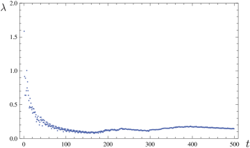
Figure 2: The Lyapunov exponent $\lambda$ graph as function of time $t$ for $z=1.01$, $E=20,$ and $\ell=1$. In this figure, the Lyapunov exponent converges asymptotically to one positive value of $0.15$.

5 Conclusion

In this work, we investigated the chaotic behavior of the circular test string moving in the Lifshitz background, which allows the scaling anisotropy between space and time whenever $z\neq 1$. Most of all, we considered that the critical exponent $z$ defined in the Lifshitz background plays a role of the external control parameter, since our primary goal was to examine the relation between space time anisotropy and chaos. This is clearly different from the case of the literatures [15, 16, 17, 18], which were thought of the total conserved energy of the string as the external control parameter to investigate the chaotic behavior of the test string. Our numerical results obtained by using both the Poincaré section and Lyapunov exponent indicate that if $z=1$, the motion of the string is regular, while in the case slightly off $z=1$, its behavior can be irregular and chaotic.

Finally we propose that the space time anisotropy which breaks Lorentz symmetry may cause the system to be chaotic. However, in order to generalize the present result beyond the Lifshitz background that we considered in this paper, we need to explore the chaoticity of the system, which is present in the Lifshitz spacetimes for arbitrary $z$ with black hole configurations [21, 24] or naked singularity [21], which will be studied elsewhere.

We conclude a remark on the issue related to extending the Lifshitz/CFT correspondence. The authors in the literature [18] suggested the extension of AdS/CFT correspondence to include chaotic dynamics in such a way that the proper bound for the Poincaré recurrence time could be connected with the positive largest Lyapunov exponent, which describes the late time behavior of the distance between two string worldsheets as the correlator to which the worldsheets are dual. The explicit computation of the proper bound for the Poincaré recurrence time in the Lifshitz background is beyond the scope of the present paper, but nevertheless, it is worthwhile to be explored in future work.

Acknowledgements

T.M. would like to thank Prof. Yun Soo Myung for his valuable comments. This work was supported by the National Research Foundation of Korea(NRF) grant funded with grant number 2014R1A2A1A01002306. T.M. was supported by the National Research Foundation of Korea (NRF) grant funded by the Korea government (MEST) (No.2012-R1A1A2A10040499).

References

- [1] J. M. Maldacena, Adv. Theor. Math. Phys. 2, 231 (1998) [hep-th/9711200] ; Int. J. Theor. Phys. 38, 1113 (1999).
- [2] S. S. Gubser, I. R. Klebanov and A. M. Polyakov, Phys. Lett. B 428 (1998) 105 [hep-th/9802109].
- [3] E. Witten, Adv. Theor. Math. Phys. 2, 253 (1998) [hep-th/9802150].
- [4] S. A. Hartnoll, Class. Quant. Grav. 26 (2009) 224002 [arXiv:0903.3246 [hep-th]].
- [5] J. McGreevy, Adv. High Energy Phys. 2010, 723105 (2010) [arXiv:0909.0518 [hep-th]].
- [6] P. Koroteev and M. Libanov, JHEP 0802 (2008) 104 [arXiv:0712.1136 [hep-th]].
- [7] K. Balasubramanian and J. McGreevy, Phys. Rev. Lett. 101, 061601 (2008) [arXiv:0804.4053 [hep-th]].
- [8] S. Kachru, X. Liu and M. Mulligan, Phys. Rev. D 78, 106005 (2008) [arXiv:0808.1725 [hep-th]].
- [9] K. Copsey and R. Mann, JHEP 1103 (2011) 039 [arXiv:1011.3502 [hep-th]].
- [10] G. T. Horowitz and B. Way, Phys. Rev. D 85, 046008 (2012) [arXiv:1111.1243 [hep-th]].
- [11] N. Bao, X. Dong, S. Harrison and E. Silverstein, Phys. Rev. D 86, 106008 (2012) [arXiv:1207.0171 [hep-th]].
- [12] S. Harrison, S. Kachru and H. Wang, arXiv:1202.6635 [hep-th].
- [13] B. Carter, Phys. Rev. 174, 1559 (1968).
- [14] E. Hackmann, V. Kagramanova, J. Kunz and C. Lammerzahl, Phys. Rev. D 78, 124018 (2008) [Erratum-ibid. 79, 029901 (2009)] [arXiv:0812.2428 [gr-qc]].
- [15] A. V. Frolov and A. L. Larsen, Class. Quant. Grav. 16 (1999) 3717 [gr-qc/9908039].
- [16] P. Basu, D. Das and A. Ghosh, Phys. Lett. B 699 (2011) 388 [arXiv:1103.4101 [hep-th]].
- [17] P. Basu and L. A. Pando Zayas, Phys. Lett. B 700 (2011) 243 [arXiv:1103.4107 [hep-th]].
- [18] L. A. Pando Zayas and C. A. Terrero-Escalante, JHEP 1009 (2010) 094 [arXiv:1007.0277 [hep-th]].
- [19] A. N. Kolmogorov, Dokl. Akad. Nauk SSSR 98, 527 (1954); V. I. Arnold, Russ. Math. Surv. 18, 13 (1963); J. Moser, Nachr. Akad. Wiss. Göttingen Math. Phys. K1 II 1 (1962); C. Eugene Wayne, An introduction to KAM theory, Dynamical systems and probabilistic methods in partial differential equations (Berkeley, CA, 1994).
- [20] R. C. Hilborn, Chaos and Nonlinear Dynamics, 2nd ed. (Oxford University Press, 2000); E. Ott, Chaos in Dynamical Systems, 2nd ed. (Cambridge University Press, 2002).
- [21] J. Tarrio and S. Vandoren, JHEP 1109 (2011) 017 [arXiv:1105.6335 [hep-th]].
- [22] J. C. Sprott, “Chaos and Time-Series Analysis,” Oxford University Press, 2003.
- [23] J. C. Sprott, “Numerical Calculation of Largest Lyapunov Exponent,” http://sprott.physics.wisc.edu/chaos/lyapexp.htm
- [24] M. Taylor, arXiv:0812.0530 [hep-th]; U. H. Danielsson and L. Thorlacius, JHEP 0903 (2009) 070 [arXiv:0812.5088 [hep-th]]; R. B. Mann, JHEP 0906 (2009) 075 [arXiv:0905.1136 [hep-th]]; M. H. Dehghani and R. B. Mann, JHEP 1007 (2010) 019 [arXiv:1004.4397 [hep-th]]; W. G. Brenna, M. H. Dehghani and R. B. Mann, Phys. Rev. D 84, 024012 (2011) [arXiv:1101.3476 [hep-th]]; M. H. Dehghani, R. B. Mann and R. Pourhasan, Phys. Rev. D 84, 046002 (2011) [arXiv:1102.0578 [hep-th]].