IFUP-TH/2014-16

Abstract
We discuss the large-distance approximation of the monopole-vortex complex soliton in a hierarchically broken gauge system, $SU(N+1)\to SU(N)\times U(1)\to{\bf 1}$, in a color-flavor locked $SU(N)$ symmetric vacuum. The (’t Hooft-Polyakov) monopole of the higher-mass-scale breaking appears as a point and acts as a source of the thin vortex generated by the lower-energy gauge symmetry breaking. The exact color-flavor diagonal symmetry of the bulk system is broken by each individual soliton, leading to nonAbelian orientational $CP^{N-1}$ zeromodes propagating in the vortex worldsheet, well studied in the literature. But since the vortex ends at the monopoles these fluctuating modes endow the monopoles with a local $SU(N)$ charge. This phenomenon is studied by performing the duality transformation in the presence of the $CP^{N-1}$ moduli space. The effective action is a $CP^{N-1}$ model defined on a finite-width worldstrip.

1 Introduction

The idea of nonAbelian monopoles and the associated concept of nonAbelian duality has proven to be peculiarly elusive. The exact Seiberg-Witten solutions and its generalizations in the context of ${\cal N}=2$ supersymmetric theories [1]-[2] show that the massless monopoles appearing at various simple singularities of the quantum modiuli space of vacua (QMS) are Abelian. There are clear evidences [1]-[3] that they are indeed the ’t Hooft-Polyakov monopoles becoming light by quantum effects. This has (mis-)led some people to believe that the monopoles seen in the low-energy dual theories of the soluble ${\cal N}=2$ models are always Abelian. Actually, in many degenerate singularities where Abelian vacua coalesce (e.g., at certain values of the bare masses and/or at special points of the vacuum moduli space), nonAbelian monopoles regularly make appearance [4]-[5] as dual, massless degrees of freedom. They correctly describe the infrared phenomena such as confinement and global symmetry breaking . NonAbelian monopoles are also known to appear in infrared-fixed-points of ${\cal N}=1$ supersymmetric theories, those in Seiberg’s conformal window (${\cal N}=1$ SQCD, for $\tfrac{3}{2}N_{c}<N_{f}<3N_{c}$) [6] being the most celebrated examples . Even more intriguing is the situation in highly singular vacua occurring in the context of ${\cal N}=2$ SQCD for some critical quark mass in $SU(N)$ theories [7, 8] or in the massless limit of $SO(N)$ or $USp(2N)$ theories [4, 9, 10]. These infrared-fixed-point SCFT’s are described by a set of relatively nonlocal and strongly-coupled monopoles and dyons, and it is quite a nontrivial matter to analyze what happens when a ${\cal N}=1$ deformation is introduced in the theory. Is the system brought into confinement phase? And if so, how is it described? Only quite recently some progress was made concerning these questions [11], taking full advantage of some beautiful results of Argyres, Gaiotto, Seiberg, Tachikawa and others [12, 13, 14]. Confinement vacua near such highly singular SCFT exhibit interesting features which could provide important hints about the not-yet-known confinement mechanism in QCD.

Leaving aside this deep issue here, the point is that appearance of the nonAbelian monopoles as infrared degrees of freedom is quite common in strongly interacting nonAbelian gauge theories. What is lacking still is the understanding of these quantum objects, or in other words, of their semi-classical origin. This question is a relevant one, in view of the difficulties associated with the straightforward idea of semi-classical nonAbelian monopoles [15, 16, 17].

It is our aim in this paper to take a few more steps towards elucidating the mysteries of nonAbelian duality. For this purpose we study a system with hierarchical symmetry breaking

$$SU(N+1)_{\rm color}\otimes SU(N)_{\rm flavor}\stackrel{{\scriptstyle v_{1}}}{{\longrightarrow}}(SU(N)\times U(1))_{\rm color}\otimes SU(N)_{\rm flavor}\stackrel{{\scriptstyle v_{2}}}{{\longrightarrow}}SU(N)_{C+F}\ ,$$ (1)

with

$$v_{1}\gg v_{2}\ ,$$ (2)

as in [18]-[22]. The homotopy group associated with the gauge symmetry breaking,

$$\Pi_{2}(SU(N+1)/SU(N)\times U(1))\sim{\mathbbm{Z}}$$ (3)

supports monopoles with quantized magnetic charges, whereas the low-energy $U(N)$ symmetry breaking with

$$\Pi_{1}(SU(N)\times U(1))\sim{\mathbbm{Z}}$$ (4)

implies vortices. As neither of them exists in the full theory,

$$\Pi_{2}(SU(N+1))=\Pi_{1}(SU(N+1))={\mathbbm{1}},$$ (5)

the vortex must end: the endpoints are the monopoles. This fact can be rephrased by the short exact sequence of the associated homotopy groups:

$${\mathbbm{1}}=\Pi_{2}(SU(N+1))\to\Pi_{2}(\tfrac{SU(N+1)}{SU(N)\times U(1)})\to\Pi_{1}(SU(N)\times U(1))\to\Pi_{1}(SU(N+1))={\mathbbm{1}}\;.$$ (6)

The fact that neither monopole or vortex exist as stable solitons of the full theory does not prevent us from investigating these configurations. The idea is to keep the mass-scale hierarchy $v_{1}\gg v_{2}$ as strong as we wish, so that the concept of monopole or vortex is as good as any approximation used in physics .

Note that the topological classifications such as Eqs. (3), (4), are not fine enough to specify the minimum-energy configuration in each class. There are continuously infinite degeneracy of such minimum configurations due to the breaking of the exact global color-favor $SU(N)_{C+F}$ symmetry by the vortex and monopole. The connection implied by Eq. (6) however means that each minimal vortex configuration of the minimum class of Eq. (4) ends at a monopole of the miminum class Eq. (4). This connection endows the monopole with the same $CP^{N-1}$ orientation moduli of the nonAbelian vortex.

The new $SU(N)$ quantum number of the monopole arises as the isometry group of this $CP^{N-1}$ moduli space, following from the exact color-flavor symmetry of the original gauge system. The monopole transforms in the fundamental representation of this $SU(N)$. Fluctuation of the monopole $SU(N)$ charge excites the well-known non-Abelian vortex zero modes [25, 18], which propagate as massless particles in the 2D worldsheet. One way of thinking about this result is that the non-normalizable $3D$ gauge zero modes of the monopole, when dressed by flavor charges, turn into normalizable $2D$ modes on the vortex world sheet.

The new $SU(N)$ symmetry is a result of the color-flavor combined transformations acting on the soliton monopole-vortex configurations: the latter is a nonlocal field transformation. Nevertheless, in the dual description the new $SU(N)$ acts locally on the monopole. This is typical of electromagnetic duality.

This $SU(N)$ charge of the monopole is a confined charge, as the excitation does not propagate outside the monopole-vortex-antimonopole complex. The $M-V-{\bar{M}}$ complex is a singlet as a whole. The monopoles appear as confined objects, the vortex playing the role of the confining string. This is correct as the original $SU(N)$ gauge system is in a completely broken, Higgs phase. The dual system must be in confinement phase.

The following is an attempt to make these ideas a little more concrete.

2 The model

Our aim is to study a simplest possible model which realizes the hierarchical symmetry breaking Eq.(1) in which the light matter and gauge fields interact with the monopole arising from the higher-mass symmetry breaking. The action can be taken in the form,

$$\mathcal{L}=-\frac{1}{4}\left(F_{\mu\nu}\right)^{2}+|{\cal D}_{\mu}\phi|^{2}+\sum_{I=1}^{N_{F}}\left|{\cal D}_{\mu}q_{I}\right|^{2}-V(\phi,q)\,,$$ (7)

where $\phi$ is a scalar field in the adjoint representation of $SU(N+1)$, $q_{I}$, where $I=1,2,\ldots,N_{F}=N$, are a set of other scalar fields, in the fundamental representation. Inspired by the ${\cal N}=2$ theories, we take

$$V=\sum_{A}\left|\mu\,\phi^{A}+\lambda\,{q}_{I}^{\dagger}\,T^{A}q^{I}\right|^{2}+\sum_{I,i}\left|(T^{A}\phi^{A}+m_{I})_{ij}\,q_{j}^{I}\right|^{2}\,.$$ (8)

where $m_{1},m_{2},\ldots m_{N}$ are the (bare) masses of the scalar fields $q$, and $\mu\ll|m_{I}|$. The quartic coupling $\lambda$ does not play a particular role in our discussion below, and will be set to unity. In order to attain the minimum of the potential, $V=0$, the scalar field $q_{I}$ is either a non vanishing eigenvector of the $\phi$ with eigenvalue, $m_{I}$, or must vanish. We shall take the equal mass limit, $m_{1}=m_{2}=\ldots=m_{N}=m_{0}$ and choose to work in the vacuum with

$$\langle\phi\rangle=\langle\phi^{A}T^{A}\rangle=m_{0}\,\left(\begin{array}[]{cc}N&\\ &-{\mathbbm{1}}_{N}\end{array}\right)$$ (9)

breaking the $SU(N+1)$ gauge symmetry to $SU(N)\times U(1)$. An inspection of the second term of the potential shows that the first (color) component of the scalars $q_{I}$ becomes massive for all $I$ (with vanishing VEV), with mass

$$v_{1}\equiv m_{0}(N+1),$$ (10)

and decouples at mass scales lower than that. The other components are nontrivial eigenvectors $q_{I}$ of $\phi$. $N_{f}=N$ eigenvectors can be taken to be orthogonal to each other, $\langle q_{I}^{a}\rangle=c_{I}\,\delta^{a}_{I}.$ The first term tells

$$\hbox{\rm tr}\,t^{A}\sum_{I}(\,q_{I}\,q^{\dagger\,I})=0\;,\qquad t^{A}\subset SU(N),$$ (11)

that is, $\sum_{I}q_{I}\,q^{\dagger\,I}\propto{\mathbbm{1}}_{N}$. In other words, all $c_{I}$’s are equal. Their normalization is fixed by the $A=0$ (see Eq. (13)) term to be

$$\langle q_{I}^{a}\rangle=v_{2}\,\delta^{a}_{I}\;,\qquad v_{2}\equiv\sqrt{2(N+1)\mu m_{0}}\ll v_{1}\,.$$ (12)

showing that the gauge symmetry is completely broken at low energies, leaving however the color-flavor diagonal symmetry $SU(N)_{C+F}$ unbroken.

3 Point: the monopole

Let us write the VEV of $\phi$ as

$$\phi(x)=v_{1}\,M(x),\qquad\langle M\rangle=\sqrt{\frac{2N}{N+1}}\,T^{(0)},\qquad T^{(0)}=\frac{1}{\sqrt{2N(N+1)}}\left(\begin{array}[]{cc}N&\\ &-{\mathbbm{1}}_{N}\end{array}\right)\;.$$ (13)

As the system admits the topological defect (the monopole), we need to retain the degrees of freedom corresponding to the nontrivial winding

$$\Pi_{2}(SU(N+1)/U(N))={\mathbbm{Z}}$$

that is,

$$M(x)=\sqrt{\frac{2N}{N+1}}\,U(x)\,T^{(0)}\,U^{\dagger}(x),\qquad\hbox{\rm Tr}\,(T^{(0)})^{2}=\frac{1}{2}\;.$$ (14)

The $M(x)$ ($U(x)$) field defines the direction of the symmetry breaking,

$$SU(N+1)/U(N)\sim CP^{N},$$ (15)

and can be expressed by a complex $(N+1)$-component vector field $z(x)$ as

$$M=z\,{\bar{z}}-\frac{1}{N+1}{\mathbbm{1}},\qquad{\bar{z}}\,z=1.$$ (16)

By introducing the $N+1$ orthonormal eigenvectors of $M$, $z(x)$ and $e_{i}(x)$ ($i=1,2,\ldots N$) with eigenvalues,

$$\frac{N}{N+1},\quad-\frac{1}{N+1},\quad-\frac{1}{N+1},\quad\ldots,\quad-\frac{1}{N+1},$$

$U(x)$ can be written as

$$U(x)=\left(\left(\begin{array}[]{c}\\ z\\ \\ \end{array}\right)\left(\begin{array}[]{c}\\ e_{1}\\ \\ \end{array}\right)\cdots\left(\begin{array}[]{c}\\ e_{N}\\ \\ \end{array}\right)\right).$$ (17)

The $z^{a}$ and $e^{a}_{i}$ can be thought of as local vielbeins [26].

The gauge field can be taken so as to satisfy the so-called Cho gauge [27]

$$(D_{\mu}\phi)/v_{1}=D_{\mu}M=\partial_{\mu}M-ig\,[A_{\mu},M]=0\;,$$ (18)

which amounts to the low-energy (large distance) approximation where the monopole appears as a point. Namely, only the winding directions, $SU(N+1)/SU(N)\times U(1)\sim CP^{N}$, are kept as the dynamical degrees of freedom associated with the monopole. Explicitly, we take the gauge field in the form,

$$A_{\mu}=C_{\mu}\,M(x)+\frac{i}{g}\,[M(x),\partial_{\mu}M(x)]+B_{\mu},$$ (19)

where

$${B}_{\mu\,b}^{a}=\sum_{i,j=1}^{N}e_{i}^{a}b^{i}_{\mu\,j}{\bar{e}}^{j}_{b}\;,\qquad a,b=1,2,\ldots,N+1\;.$$ (20)

$C_{\mu}$ is the Abelian gauge field in the direction of the scalar VEV, $b^{i}_{\mu\,j}$ are the components of the gauge fields of the ”unbroken” $SU(N)$, and $i\,[M(x),\partial_{\mu}M(x)]/g$ represents the monopole field. It can be easily checked that the connection Eq. (19) indeed satisfies the gauge condition Eq. (18).

Note that the Cho condition Eq. (18) does not uniquely determine the component of the gauge field $A_{\mu}$ orthogonal to $zz^{\dagger}$, as

$$[e(\ldots){\bar{e}},M]=0\;.$$

In Eq. (19) we have chosen $A_{\mu}$ so that it contains precisely the monopole configuration

$$i\,[M(x),\partial_{\mu}M(x)]\subset su(2)\subset su(N+1),$$ (21)

besides the ”unbroken” massless $SU(N)$ gauge fields $b_{\mu\nu}$ and the Abelian gauge field $C_{\mu}$ (the $U(1)$ rotations around $M$ direction).

The transformation properties of the gauge connection above have been studied in [26]. Under the U($1$) transformation around the $M$ direction,

$$U=e^{i\alpha M}=e^{i\alpha\frac{N}{N+1}}z{\bar{z}}+e^{-i\alpha\frac{1}{N+1}}e{\bar{e}}\;$$ (22)

the Abelian field $C_{\mu}$ transforms as expected:

$$C_{\mu}\to C_{\mu}-\,\partial_{\mu}\alpha\;.$$ (23)

Under the $SU(N)$ transformations commuting with $M$,

$$U=\exp(i\,\omega^{\textsf{A}}e\,t^{\textsf{A}}\bar{e})=e\,\Omega\,\bar{e}+z\bar{z}\;,\qquad\Omega=\exp(i\,\omega^{\textsf{A}}t^{\textsf{A}})\;.$$ (24)

where $(t^{\textsf{A}})^{i}_{j}$ ($i,j=1,2,\ldots N$) are $SU(N)$ generators, $b_{\mu}$ transforms as the usual nonAbelian gauge field:

$$b_{\mu}\to b^{U}_{\mu}=\Omega\,b_{\mu}\Omega^{\dagger}-i\,\partial_{\mu}\Omega\,\Omega^{\dagger}\;.$$ (25)

3.1 The minimal monopoles

For the minimal monopole one can choose $z$ and one of the $e$’s to live in a $SU(2)\in SU(N+1)$ subgroup and consider their winding only [26],

$$z=\left(\begin{array}[]{c}\cos\frac{\theta}{2}\\ 0\\ \vdots\\ e^{i\varphi}\sin\frac{\theta}{2}\\ 0\\ \vdots\end{array}\right)\;,\qquad e_{i}=\left(\begin{array}[]{c}-e^{-i\varphi}\sin\frac{\theta}{2}\\ 0\\ \vdots\\ \cos\frac{\theta}{2}\\ 0\\ \vdots\end{array}\right)\;;$$ (26)

$$e_{j}^{a}=\delta_{j+1}^{a},\qquad a=1,\ldots N+1,\quad j=1,\ldots,N,\quad j\neq i\;.$$ (27)

In other words, only the vielbeins $z$ and $e_{i}$ in the first and $(i+1)$-th color components are relevant for the monopole. They take the form of normalized spin $1/2$ wave functions, spin up for $z$, spin down for $e_{i}$, all the rest of the components being zero. Other vielbeins $e_{j}$, $j\neq i$, have canonical, orthonormal unit vector forms. $z$ and $e$’s are not independent but are related by the completeness and orthonormality conditions

$$z^{a}{\bar{z}}_{b}+\sum_{i=1}^{N}e_{i}^{a}{\bar{e}}^{i}_{b}=\delta^{a}_{b},\qquad{\bar{z}}_{a}z^{a}=1,\quad{\bar{e}}^{i}_{a}e_{j}^{a}=\delta^{i}_{j}\;,\quad{\bar{z}}_{a}e^{a}_{i}=0\;.$$ (28)

but it is an arbitrary choice which of the vielbeins $e$ winds together with $z$.

For the minimal monopole, Eq. (26), the $(N+1)\times(N+1)$ matrix field $M$ takes the form,

$$M=\phi/v_{1}=z\,{\bar{z}}-\frac{1}{N+1}{\mathbbm{1}}=\frac{{\bf n}\cdot\tau}{2}+\frac{{\bf 1}_{1,i+1}}{2}-\frac{{\bf 1}}{N+1},$$ (29)

$${\bf n}=\frac{\bf r}{r}=(\sin\theta\cos\varphi,\sin\theta\sin\varphi,\cos\theta)\;,$$ (30)

where $\tau$ and ${\bf 1}_{1,i+1}$ are the Pauli matrices and the $2\times 2$ unit matrix in the $(1,i+1)$ subspace. The monopole part of the gauge field Eq. (19) is simply:

$$A_{\mu}^{(monopole)}=\frac{i}{g}[M,\partial_{\mu}M]=-\frac{\tau}{2g}\cdot({\bf n}\times\partial_{\mu}{\bf n})\;,$$ (31)

which is indeed the singular Wu-Yang monopole lying in the $su(2)\subset su(N+1)$ algebra in the $(1,i+1)$ subspace. This is nothing but the asymptotic form of the ’t Hooft-Polyakov monopole, far from its center ($R\gg 1/v_{1}$).

Rotating this monopole field in one of the legs ($i=1,2,\ldots,N$), i.e., in the ”unbroken” $SU(N)$ group, amounts to the straightforward idea of nonAbelian monopoles: a set of configurations of degenerate mass, which apparently belong to the fundamental representation of the $SU(N)$. A closer examination however reveals the well-known difficulties (e.g., the topological obstruction [15]). Any deeper understanding of the non-Abelian monopole notion necessarily involves an exact flavor symmetry, as is fairly well known, and our following discussion is precisely based on such a consideration.

The gauge field tensor can be calculated straightforwardly:

$$(F_{\mu\nu})^{a}_{b} = \left(\partial_{\mu}A_{\nu}-\partial_{\nu}A_{\mu}-ig\,[A_{\mu},A_{\nu}]\right)^{a}_{b}$$

$$= z^{a}\,\{\frac{M_{\mu\nu}}{2}+\frac{N}{N+1}C_{\mu\nu}\}{\bar{z}}_{b}+e^{a}_{i}\,\{(K_{\mu\nu})^{i}_{j}-\frac{1}{N+1}C_{\mu\nu}\delta^{i}_{j}+(b_{\mu\nu})^{i}_{j}+(h_{\mu\nu})^{i}_{j}\}\,{\bar{e}}^{j}_{b}$$

where

$$C_{\mu\nu}=\partial_{\mu}C_{\nu}-\partial_{\nu}C_{\mu},\qquad M_{\mu\nu}\equiv\partial_{\mu}N_{\nu}-\partial_{\nu}N_{\mu},\qquad N_{\mu}\equiv\frac{2i}{g}\,{\bar{z}}_{a}\partial_{\mu}z^{a}\;;$$ (33)

$$(K_{\mu\nu})^{i}_{j}=\partial_{\mu}(P_{\nu})^{i}_{j}-\partial_{\nu}(P_{\mu})^{i}_{j}-i\,g\,[P_{\mu},P_{\nu}]^{i}_{j}\;,\qquad(P_{\mu})^{i}_{j}=\frac{i}{g}\,{\bar{e}}^{i}_{a}\partial_{\mu}e^{a}_{j}\;;$$ (34)

$$b_{\mu\nu}=\partial_{\mu}b_{\nu}-\partial_{\nu}b_{\mu}-i\,g\,[b_{\mu},b_{\nu}]\;;\qquad h_{\mu\nu}=-ig\left([P_{\mu},b_{\nu}]-[P_{\nu},b_{\mu}]\right)\;.$$ (35)

4 The matter coupling: vortex and the low-energy effective action

The scalar matter fields $q$ in the fundamental representation of $SU(N+1)$ (“squarks”) can be decomposed as

$$q^{a}_{I}(x)=z^{a}\chi_{I}+e^{a}_{i}\,\eta^{i}_{I}\;,$$ (36)

where

$$a=1,2,\ldots,N+1\;,\quad i=1,2,\ldots,N\;,\quad I=1,2,\ldots N_{f}=N\;,$$ (37)

namely, into the component parallel to the symmetry breaking direction, $z$, (see Eq. (15)) and those orthogonal to it, $e^{a}_{i}$’s.

As one sees from the fact that

$$U^{\dagger}\,q_{I}=U^{\dagger}(z\chi_{I}+e\eta_{I})=\left(\begin{array}[]{c}\chi_{I}\\ \eta^{1}_{I}\\ \vdots\\ \eta^{N}_{I}\end{array}\right)\;,$$ (38)

$\chi$ and $\eta$’s are nothing but the scalar field components in the singular gauge of the monopole (in which the adjoint scalar field does not wind and approaches a fixed VEV in all directions). The monopole fields $N_{\mu}$, $P_{\mu}$ which couple to the projected scalars $\chi$ and $\eta$ have automatically the (asymptotic) form of the ’t Hooft-Polyakov monopole in the singular gauge. As is well known the monopole field develops a Dirac string singularity attached to it in such a gauge.

By using the orthonormality and completeness of the vielbeins, one arrives at the following decomposition

$$\{(\partial_{\mu}-igA_{\mu})\,q_{I}\}^{a} = z^{a}\{\partial_{\mu}\chi_{I}+({\bar{z}}\,\partial_{\mu}z)\chi_{I}-ig\frac{N}{N+1}\,C_{\mu}\chi_{I}\}$$ (39)

$$+ e^{a}_{j}\,\{(\partial_{\mu}-i\,g\,b_{\mu})^{j}_{k}\,\eta^{k}_{I}+{\bar{e}}^{j}_{b}\,\partial_{\mu}e_{i}^{b}\,\eta_{I}^{i}+i\frac{g}{N+1}\,C_{\mu}\eta_{I}^{j}\}\;.$$

Both $\chi$ and $\eta$ have $U(1)$ electric charge, whereas only the $\eta$ fields carry non-Abelian $SU(N)$ charges. The matter kinetic term thus decomposes as

$$\hbox{\rm Tr}\,|(\partial_{\mu}-igA_{\mu})\,q_{I}|^{2} = |\partial_{\mu}\chi_{I}-ig\frac{N_{\mu}}{2}\chi_{I}-ig\frac{N}{N+1}\,C_{\mu}\chi_{I}|^{2}$$ (40)

$$+ |(\partial_{\mu}-i\,g\,b_{\mu})^{j}_{k}\,\eta^{k}_{I}-ig(P_{\mu})^{j}_{i}\,\eta_{I}^{i}+i\frac{g}{N+1}\,C_{\mu}^{(0)}\eta_{I}^{j}|^{2}\;.$$

The minimization of the potential Eq. (8) leads to

$$|(\phi+m_{0}{\mathbbm{1}})\,q|^{2}=|(m_{0}(N+1)M+m_{0}{\mathbbm{1}})\,q|^{2}=|\,m_{0}(N+1)\,\chi_{I}\,|^{2}\;,$$ (41)

which shows that the scalars in the $z$ direction, $\chi_{I}$, are massive, which can be integrated out. The low-energy effective action considered below describes the physics of the massless fields $\eta_{I}$, the ”unbroken” gauge fields $b_{\mu}$ and the monopole $P_{\mu}$ ,

$${\cal L} = -\frac{1}{2}\hbox{\rm Tr}F_{\mu\nu}F^{\mu\nu}+\sum_{I,j}\left|(\partial_{\mu}-i\,g\,b_{\mu})^{j}_{k}\,\eta^{k}_{I}-ig(P_{\mu})^{j}_{i}\,\eta_{I}^{i}+i\frac{g}{N+1}\,C_{\mu}\,\eta_{I}^{j}\right|^{2}-V_{\eta}\;$$ (42)

$$\equiv {\cal L}^{gauge}+{\cal L}^{scalar}-V_{\eta}\;,$$

where

$$\hbox{\rm Tr}F_{\mu\nu}F^{\mu\nu} = (\frac{M_{\mu\nu}}{2}+\frac{N}{N+1}C_{\mu\nu})^{2}+$$ (43)

$$+ \hbox{\rm tr}\,\left((K_{\mu\nu})^{i}_{j}-\frac{1}{N+1}C_{\mu\nu}\delta^{i}_{j}+(b_{\mu\nu})^{i}_{j}+(h_{\mu\nu})^{i}_{j}\right)^{2}$$

and $M_{\mu\nu},(K_{\mu\nu})^{i}_{j},C_{\mu\nu},(b_{\mu\nu})^{i}_{j},(h_{\mu\nu})^{i}_{j}$ are defined in Eqs. (33)-(35). For the minimum monopole lying in the $(1,i+1)$ $su(2)$ subalgebra, (Eqs. (26), (30)),

$${\bar{z}}\,\partial_{\varphi}z=i\frac{1-\cos\theta}{2},\qquad{\bar{e}}^{i}\,\partial_{\varphi}e_{i}=-{\bar{z}}\,\partial_{\varphi}z\ =-i\frac{1-\cos\theta}{2},\quad({\rm no~{}sum~{}over~{}}i)\;,$$ (44)

$${\bar{e}}^{j}\,\partial_{\mu}e_{i}=0,\quad j\neq i,\qquad{\bar{z}}\,\partial_{\theta}z={\bar{e}}^{i}\,\partial_{\theta}e_{i}=0\;.$$ (45)

Eq.(44) is precisely the Wu-Yang monopole in the singular gauge, with Dirac string along the negative $z$ axis, $z\in(-\infty,0)$,

$$A_{\varphi}^{Dirac}=\frac{1-\cos\theta}{\rho g}\;,$$ (46)

where $\rho$ is the distance from the $z$ axis. Taking into account the factor $\tfrac{1}{2}$ due to the $su(2)\subset su(N+1)$ embedding $\tfrac{\tau}{2}$, we see that the light scalars $\eta$ is coupled to such a monopole only through the $(P_{\mu})^{i}_{i}$ term:

$$P_{\mu}=\frac{1}{2}\left(\begin{array}[]{ccccc}\ddots&&&&\\ &0&&&\\ &&A_{\varphi}^{Dirac}&&\\ &&&0&\\ &&&&\ddots\end{array}\right)$$ (47)

The minimization of the potential $V_{\eta}$ then leads to the VEV (Appendix A)

$$\eta^{i}_{I}=\delta^{i}_{I}\,{v_{2}}\;.$$ (48)

This VEV brings the low-energy system into a color-flavor locked, completely Higgsed phase. In such a vacuum, due to the exact flavor $SU(N)_{C+F}$ symmetry, broken by individual vortex solution, the latter develops non-Abelian orientational zero modes.

4.1 Symmetries

The low-enegy system Eq. (42) arose from the gauge symmetry breaking,

$$SU(N+1)\to SU(N)\times U(1)$$ (49)

and if the monopole fields $N_{\mu}$ and $P_{\mu}$ are dropped it would be the standard $SU(N)\times U(1)$ gauge theory action. It is clear, however, that in the presence of a minimal monopole, (Eqs. (26), (30), (31)), the local color $SU(N)$ symmetry is broken by the specific direction $M(x)=z{\bar{z}}-(1/(N+1)){\mathbbm{1}}_{N+1}$ the monopole points. Attempts to define a global unbroken ”orthogonal” $SU(N)$ group in the presence of the monopole background, lead inevitably to the well-known difficulties [15, 17].

There are however some local and global symmetries which are left intact. In order to fix the idea, let us take the monopole in the $(a,b)=1,2$ color subspace. That is, we choose particular monopole orientation with $i=1$, in Eqs. (26), (30), (31). In this case the only nonvanishing component of $P_{\mu}$ is:

$$P^{1}_{\varphi\,1}=\frac{i}{g}\,{\bar{e}}^{1}\,\partial_{\varphi}e_{1}=-\frac{i}{g}\,{\bar{z}}\,\partial_{\varphi}z\ =\frac{1-\cos\theta}{2g},\qquad P_{\mu\,i}^{j}=0,\quad i\neq 1,\,{\rm or}\,\,j\neq 1\;.$$ (50)

The action Eq. (42), Eq. (43) is invariant under

(i)

a local $U(1)$ symmetry:

$$\eta^{i}\to e^{i\alpha}\eta^{i},\qquad C_{\mu}\to C_{\mu}-\beta\,\partial_{\mu}\alpha\;,\qquad\beta=(N+1)/g\;;$$ (51)

(ii)

a local $U(1)$ symmetry:

$$\eta\to U\eta,\qquad b_{\mu}\to U(b_{\mu}-\frac{i}{g}\partial_{\mu})U^{\dagger}\;,\qquad U=\left(\begin{array}[]{cc}e^{i(N-1)\gamma}&0\\ 0&e^{-i\gamma}\,{\mathbbm{1}}_{N-1}\end{array}\right),$$ (52)

(iii)

a local $SU(N-1)$ symmetry:

$$\eta\to U\eta,\qquad b_{\mu}\to U(b_{\mu}-\frac{i}{g}\partial_{\mu})U^{\dagger}\;,\qquad U=\left(\begin{array}[]{cc}1&0\\ 0&V_{N-1}\end{array}\right)\;,$$ (53)

(ii), (iii) are subgroups of the local $SU(N)$ group broken by the particular orientation of the monopole.

Finally, the action is invariant under

(iv)

a global flavor $SU(N)_{F}$ symmetry:

$$\eta\to\eta\,{\cal U}^{\dagger},\qquad{\cal U}\in SU(N)\;.$$ (54)

All the local ((i)-(iii)) and global ((iv)) symmetries are broken by the VEV of the scalars $\eta$, Eq. (48). However there remains

(v)

an exact global color-flavor diagonal $SU(N)$ symmetry

$$\eta\to{\cal U}\,\eta\,{\cal U}^{\dagger},\qquad P_{\mu}\to{\cal U}\,P_{\mu}\,{\cal U}^{\dagger},\qquad b_{\mu}\to{\cal U}\,b_{\mu}\,{\cal U}^{\dagger},\qquad{\cal U}\in SU(N)\;.$$ (55)

Note that $K_{\mu\nu},b_{\mu\nu},h_{\mu\nu}$ all transform covariantly under Eq. (55).

In particular, the invariance of the action under (v) requires that, together with the light matter and gauge fields, the monopole $P_{\mu}=(i/g)\,{\bar{e}}\,\partial_{\mu}e$ be also transformed with ${\cal U}$.

4.2 Monopole-vortex soliton complex

If it is not for the terms due to the monopole, $P_{\mu}$, $N_{\mu}$, the action in Eq. (42)(Eq. (43)), would be exactly the $SU(N)\times U(1)$ gauge theory with $SU(N)$ flavor symmetry where the vortices with nonAbelian $CP^{N-1}$ orientational zero modes has been first discovered [25, 18]. The homotopy-group argument applied to the system with hierarchical gauge symmetry breaking (Eq. (1)), tells us that the vortex must end at the monopole. The nonAbelian orientational zero modes of the vortex endow the endpoint monopoles with the same $CP^{N-1}$ zero modes.

On the other hand, if the nonAbelian gauge fields $b_{\mu}$ were neglected, the above action would reduce to the low-energy $U(1)$ theory arising from the symmetry breaking of an $SU(2)$ gauge theory. The $SU(2)$ origin of such a theory is signaled by the presence of the monopole term: performing the electromagnetic duality transformation explicitly [29], keeping account of the presence of the monopole ($SU(2)/U(1)$ winding), one gets an effective action of a static monopole acting as a source of the vortex emanating from it. This analysis was repeated in the $\theta$ vacua of the original $SU(2)$ theory [30]. The resulting equation of motion has been solved analytically, reproducing the Witten effect correctly near the monopole and showing a rather nontrivial behavior of magnetic and electric fields near the monopole-vortex complex. Our aim here is to generalize this construction to a more general setting here, where both the vortex and monopole carry nonAbelian orientational zero modes.

The fact that the low-energy vortex must end at the monopole can be seen more directly. The monopole term ${\bar{e}}\,\partial_{\mu}e$ is really a non local term: it contains the Dirac-string singularity running along the negative $z$-axis, Eq. (46). In itself, it would give rise to an infinite energy, unless the scalar field vanishes precisely along the same half line $z\in(-\infty,0)$: a vortex ending at the monopole ($z=0$) and extending to its left.

A microscopic study of such a monopole-vortex complex has been made by Cipriani et. al. [21], including the numerical determination of the field configurations interpolating the regular ’t Hooft-Polyakov monopoles to the known vortex solution in between. See Fig. 1 taken from [21]. We have not been successful so far in generalizing the derivation of the effective action for the orientational zeromodes directly from the microscopic field-matter action as done for the nonAbelian vortex [18, 24] to the present case of complex soliton of mixed codimensions.

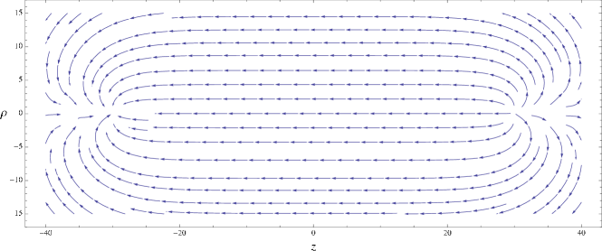
Figure 1: The magnetic field in the monopole-vortex-antimonopole soliton complex. Taken from Cipriani, et. al. [21]

Here we instead go to large distances first: the monopole is pointlike (this approximation has already been made), and the vortex is a line, without width (see Fig. 2). Implementing this last approximation the scalar field takes the form,

$$(\eta)^{i}_{I}=v_{2}\,\left(\begin{array}[]{cc}e^{i\psi}&0\\ 0&{\mathbbm{1}}_{N-1}\end{array}\right)\;,$$ (56)

whereas the relevant nonvanishing gauge fields are $C_{\mu}$, and $(b_{\mu})^{i}_{j}$ of the form,

$$(b_{\mu})^{i}_{j}=\left(\begin{array}[]{cccc}(b_{\mu})^{1}_{1}&&&\\ &(b_{\mu})^{2}_{2}&&\\ &&\ddots&\\ &&&(b_{\mu})^{N}_{N}\end{array}\right)\;.$$ (57)

The monopole term is of the form,

$$(P_{\mu})^{i}_{j}=\left(\begin{array}[]{cccc}-N_{\mu}/2&&&\\ &0&&\\ &&\ddots&\\ &&&0\end{array}\right)\;.$$ (58)

Note the matched orientation in color for the vortex and monopole in Eqs. (56) and (58).

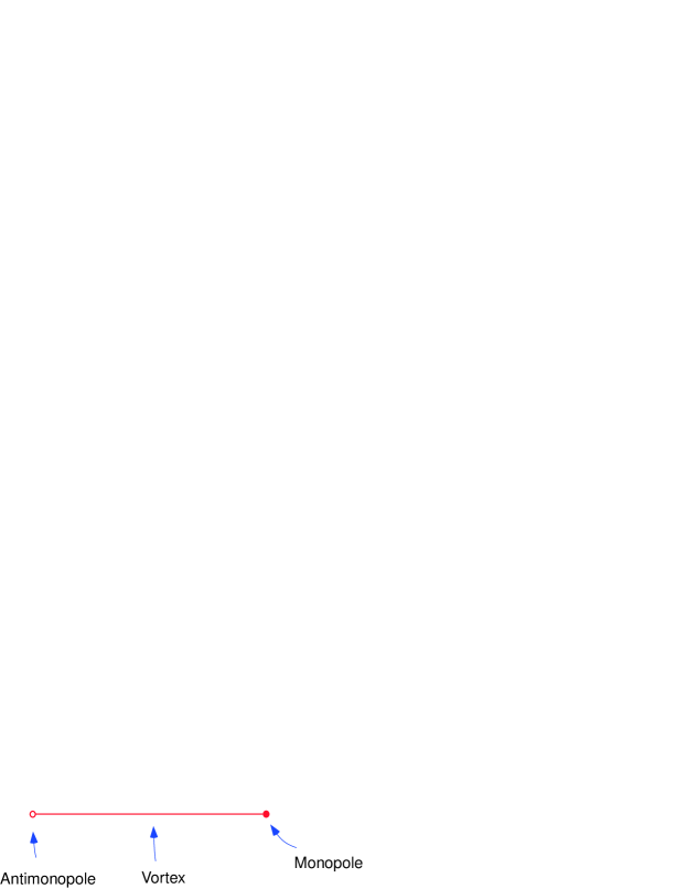
Figure 2: The monopole, vortex and anti-monopole complex of the preceding Figure, seen from large distances.

The scalar kinetic term in the action, Eq. (42), takes the form,

$${\cal L}^{scalar}=\sum_{I,j}\left|\left\{\partial_{\mu}-ig\left(\begin{array}[]{ccc}(b_{\mu})^{1}_{1}&&\\ &(b_{\mu})^{2}_{2}&\\ &&\ddots\end{array}\right)+ig\left(\begin{array}[]{ccc}-N_{\mu}/2&&\\ &0&\\ &&\ddots\end{array}\right)+\frac{ig\,C_{\mu}}{N+1}\,{\bf 1}_{N}\right\}^{j}_{i}\,\eta_{I}^{i}\,\right|^{2}\;.$$ (59)

Clearly the minimum-energy condition for $I=2,3,\ldots$ terms requires that

$$(b_{\mu})^{2}_{2}=(b_{\mu})^{3}_{3}=\ldots=(b_{\mu})^{N}_{N}=\frac{1}{N+1}\,C_{\mu}\;.$$ (60)

But as $\hbox{\rm tr}\,(b_{\mu})=0$, this means that

$$(b_{\mu})^{1}_{1}=-(N-1)(b_{\mu})^{2}_{2}=-\frac{N-1}{N+1}\,C_{\mu}\;.$$ (61)

The $I=1$ term of Eq. (59) then becomes

$${\cal L}^{scalar} = v_{2}^{2}\,\left|\{\partial_{\mu}\psi-g(b_{\mu})^{1}_{1}+g\frac{N_{\mu}}{2}+\frac{g}{N+1}\,C_{\mu}\}\,\right|^{2}$$ (62)

$$= (\partial_{\mu}\psi+g\frac{N_{\mu}}{2}+g\frac{N}{N+1}\,C_{\mu})^{2}\,v_{2}^{2}\;.$$

On the other hand, the gauge kinetic term becomes

$${\cal L}^{gauge} = -\frac{1}{2}(\frac{M_{\mu\nu}}{2}+\frac{N}{N+1}C_{\mu\nu})^{2}-\frac{1}{2}(\frac{M_{\mu\nu}}{2}+\frac{1}{N+1}C_{\mu\nu}-(b_{\mu\nu})^{1}_{1})^{2}$$ (63)

$$= -\frac{1}{4}\,(M_{\mu\nu}+\frac{2N}{N+1}C_{\mu\nu})^{2}\;.$$

Far from the vortex-monopole, the potential can be set to be equal to its value in the bulk, $V=0$. The action reduces finally to the monopole-vortex Lagrangian

$${\cal L}_{MV} = -\frac{1}{4}(M_{\mu\nu}+c_{N}\,C_{\mu\nu})^{2}+(\partial_{\mu}\psi+g\,\frac{N_{\mu}}{2}+\frac{g}{2}\,c_{N}\,C_{\mu})^{2}\,v_{2}^{2}\;,\qquad c_{N}\equiv\frac{2N}{N+1}\;$$ (64)

$$= -\frac{1}{4}(M_{\mu\nu}+C_{\mu\nu})^{2}+(\partial_{\mu}\psi+e\,N_{\mu}+e\,C_{\mu})^{2}\,v_{2}^{2}\;,$$

where in the last line we have re-normalized the Abelian gauge field $C_{\mu}$ by a constant and defined the Abelian gauge coupling $e$ by

$$c_{N}\,C_{\mu}\to C_{\mu}\;,\qquad e\equiv\frac{g}{2}.$$ (65)

In the discussion which follows, we take the monopole fields $N_{\mu}$ and $M_{\mu\nu}$ in Eq. (64) as a sum representing a monopole at ${\bf r}_{1}$ and an anti-monopole at ${\bf r}_{2}$, at the two ends of the vortex.

4.3 Orientational zeromodes

The action, Eq. (42), is invariant under the global color-flavor $SU(N)$ transformations, Eq. (55). The monopole-vortex field oriented in a particular direction, Eqs. (56)- (61) breaks this symmetry to $SU(N-1)\times U(1)$; applying ${\cal U}$ on it

$$\eta\to{\cal U}\,\eta\,{\cal U}^{\dagger},\qquad P_{\mu}\to{\cal U}\,P_{\mu}\,{\cal U}^{\dagger},\qquad b_{\mu}\to{\cal U}\,b_{\mu}\,{\cal U}^{\dagger},$$ (66)

generates a continuous set of degenerate configurations which span the coset,

$$\frac{SU(N)}{SU(N-1)\times U(1)}\sim CP^{N-1}.$$ (67)

The moduli space can be parametrized by the so-called reducing matrix [32],

$${\cal U}(B)=\begin{pmatrix}1&-B^{\dagger}\\ 0&\mathbf{1}_{N-1}\end{pmatrix}\begin{pmatrix}X^{\frac{1}{2}}&0\\ 0&Y^{-\frac{1}{2}}\end{pmatrix}\begin{pmatrix}1&0\\ B&\mathbf{1}_{N-1}\end{pmatrix}=\begin{pmatrix}X^{-\frac{1}{2}}&-B^{\dagger}Y^{-\frac{1}{2}}\\ BX^{-\frac{1}{2}}&Y^{-\frac{1}{2}}\end{pmatrix}\ ,$$ (68)

$$X\equiv 1+B^{\dagger}B\ ,\quad Y\equiv\mathbf{1}_{N-1}+BB^{\dagger}\ .$$ (69)

acting on the light fields $\eta$ and $b_{\mu}$ and on the monopole field $e$, as in Eq. (55). $B$ is an $N-1$ component complex vector, the inhomogeneous coordinates of $CP^{N-1}$.

The fields corresponding to the particular “$(1,1)$” orientation of the vortex-monopole, Eqs. (56)-(64), are of the form,

$$\eta=e^{i\psi}\,\frac{{\mathbbm{1}}_{N}+T}{2}+\frac{{\mathbbm{1}}_{N}-T}{2},\qquad\partial_{\mu}\eta=\partial_{\mu}e^{i\psi}\,\frac{{\mathbbm{1}}_{N}+T}{2}\;,$$

$$-b_{\mu}+\frac{1}{N}C_{\mu}{\mathbbm{1}}_{N}=\frac{N}{N+1}\frac{{\mathbbm{1}}_{N}+T}{2}\,C_{\mu},$$

$$P_{\mu}=-N_{\mu}\,\frac{{\mathbbm{1}}_{N}+T}{2},\qquad T\equiv\left(\begin{array}[]{cc}1&\\ &-{\mathbbm{1}}_{N-1}\end{array}\right)\;.$$ (72)

The action is then calculated to be

$$\hbox{\rm tr}\left(\frac{{\mathbbm{1}}_{N}+T}{2}\right)^{2}\cdot{\cal L}_{MV}={\cal L}_{MV}\;$$ (73)

where ${\cal L}_{MV}$ is given in Eq. (64). When a global ($x_{\mu}$-independent) color-flavor transformation ${\cal U}$ acts on it, a new solution is generated by $\{\eta,b_{\mu},P_{\mu}\}\to{\cal U}\{\eta,b_{\mu},P_{\mu}\}{\cal U}^{\dagger}\;,$ that is

$$\eta=e^{i\psi}\,\frac{{\mathbbm{1}}_{N}+{\cal U}T{\cal U}^{\dagger}}{2}+\frac{{\mathbbm{1}}_{N}-{\cal U}T{\cal U}^{\dagger}}{2},\qquad\partial_{\mu}\eta=\partial_{\mu}e^{i\psi}\,\frac{{\mathbbm{1}}_{N}+{\cal U}T{\cal U}^{\dagger}}{2}\;,$$

$$-b_{\mu}+\frac{1}{N}C_{\mu}{\mathbbm{1}}_{N}=\frac{N}{N+1}\frac{{\mathbbm{1}}_{N}+{\cal U}T{\cal U}^{\dagger}}{2}\,C_{\mu},$$

$$P_{\mu}=-N_{\mu}\,\frac{{\mathbbm{1}}_{N}+{\cal U}T{\cal U}^{\dagger}}{2}\;.$$ (74)

All the fields now have complicated, nondiagonal forms both in color and flavor spaces. Note however that

$$\Pi_{B}\equiv\frac{{\mathbbm{1}}_{N}+{\cal U}T{\cal U}^{\dagger}}{2}\;,\qquad\Pi_{O}\equiv\frac{{\mathbbm{1}}_{N}-{\cal U}T{\cal U}^{\dagger}}{2}\;,$$ (75)

act as the projection operators to the directions in color-flavor space, along the vortex-monopole orientation and perpendicular to it:

$$\Pi_{B}^{2}=\Pi_{B},\quad\Pi_{O}^{2}=\Pi_{O},\quad\Pi_{B}\cdot\Pi_{O}=0\;;\qquad\hbox{\rm tr}\,\Pi_{B}^{2}=1\;.$$ (76)

By using these, the action corresponding to the color-flavor rotated configuration, Eq. (74) is seen to be still given by

$$\hbox{\rm tr}\,{\cal L}_{scalar}\,\Pi_{B}^{2}={\cal L}_{scalar}\,,\qquad\hbox{\rm tr}\,{\cal L}_{gauge}\,\Pi_{B}^{2}={\cal L}_{gauge}\,,\qquad\hbox{\rm tr}\,\Pi_{B}^{2}\,{\cal L}_{MV}={\cal L}_{MV}\;,$$ (77)

reflecting the exact $CP^{N-1}$ moduli of the monopole-vortex solutions, following from the breaking of the exact color-flavor symmetry, Eq. (55). Therefore the $CP^{N-1}$ modes $B$ of Eqs. (66)-(69) represent exact zero modes of the monopole-vortex action, Eq. (42).

4.4 Spacetime dependent $B$

The configurations Eq. (59) - Eq. (64), or the color-flavor rotated version, Eq. (74), represents the long-distance approximation of the nonAbelian vortex with monopoles attached at the ends. They are basically an Abelian configuration embedded in a particular direction in $SU(N)_{C+F}$,

$$\Pi_{B}\equiv\frac{{\mathbbm{1}}_{N}+{\cal U}(B)T{\cal U}(B)^{\dagger}}{2}\;,$$

This is so (i.e., Abelian) even if the scalar field and gauge (and monopole) fields all have nontrivial matrix form in general in color and flavor, as they all commute with each other.

When the orientational moduli parameter $B$ is made to depend weakly on the spacetime variables $x_{\mu}$, however, such an Abelian structure cannot be maintained. The derivative acting on $\Pi_{B}$ in the scalar field induces the change of charge and current

$$\partial_{\mu}(\eta\Pi_{B})=(\partial_{\mu}\eta)\Pi_{B}+\eta\,\partial_{\mu}({\cal U}T{\cal U}^{\dagger})$$

along the vortex. It implies, through the equations of motion,

$$\frac{1}{g^{2}}{\cal D}^{i}F_{i\alpha}^{a}=i\,\sum_{I}\big{[}\eta_{I}^{{\dagger}}\,t^{a}{\cal D}_{\alpha}\eta_{I}-({\cal D}_{\alpha}\eta_{I})^{{\dagger}}t^{a}\eta_{I}\big{]},$$ (78)

new gauge field components, $A_{\alpha}^{(B)}$. This can be understood as nonAbelian Biot-Savart or Gauss’ law. Following [24] we have introduced the index $\alpha$ to indicate the two spacetime coordinates in the vortex-monopole worldsheet $\Sigma$, while indicating with $``i"$ the other two coordinates of the plane perpendicular to the vortex length. See Fig. 3. For a straight vortex in the $\hat{z}$ direction, $\alpha=3,0$ whereas $i=1,2$. By assumption $B$, hence ${\cal U}$, is a slowly varying function of $x_{\alpha}$. It is not difficult to show that $A_{\alpha}^{(B)}$ is oriented in the direction

$$A_{\alpha}^{(B)}\propto\partial_{\alpha}({\cal U}T{\cal U}^{\dagger})\,{\cal U}T{\cal U}^{\dagger}=2\,{\cal U}({\cal U}^{\dagger}\partial_{\alpha}{\cal U})_{\perp}\,{\cal U}^{\dagger},$$ (79)

in color-flavor mixed space, where

$$({\cal U}^{\dagger}\partial_{\alpha}{\cal U})_{\perp}=\frac{1}{2}({\cal U}^{\dagger}\partial_{\alpha}{\cal U}-T\,{\cal U}^{\dagger}\partial_{\alpha}{\cal U}\,T)\;.$$ (80)

$({\cal U}^{\dagger}\partial_{\alpha}{\cal U})_{\perp}$ is just the Nambu-Goldstone modes [32, 24] in a fixed vortex background, Eq. (72); as the vortex-monopole rotates (74), one has to rotate them in order to keep them orthogonal to the latter.

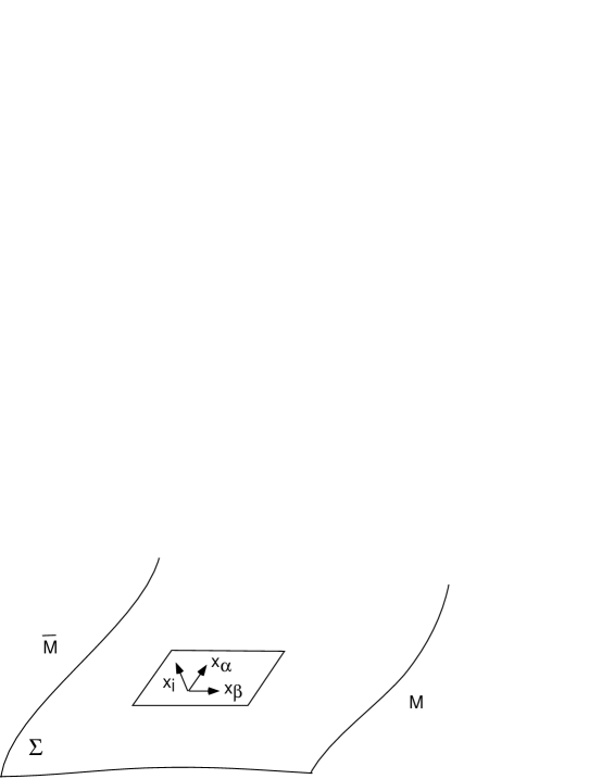
Figure 3: Worldsheet strip $\Sigma$ spanned between the worldlines of the monopole and antimonopole.

The effect is to produce the electric and magnetic fields lying in the plane perpendicular to the vortex direction, $F_{i\alpha}$, along the vortex.

By using the orthogonality relations

$$\hbox{\rm tr}\,\Pi_{B}\,\partial_{\alpha}({\cal U}T{\cal U}^{\dagger})=\hbox{\rm tr}\,\Pi_{B}\,\partial_{\alpha}({\cal U}T{\cal U}^{\dagger})\,{\cal U}T{\cal U}^{\dagger}=0,$$ (81)

it is easily seen that the terms containing the derivatives $\partial_{\mu}{\cal U}$ or $\partial_{\mu}{\cal U}^{\dagger}$ give rise to the correction

$${\cal L}({\{\eta,b_{\mu},P_{\mu}\}\to{\cal L}({\cal U}\{\eta,b_{\mu},P_{\mu}\}{\cal U}^{\dagger}})={\cal L}_{scalar}+\delta{\cal L}\;,$$

$$\Delta{\cal L}={\rm const.}\,\hbox{\rm tr}\left(\partial_{\alpha}({\cal U}T{\cal U}^{\dagger})\right)^{2}\propto\hbox{\rm tr}\left\{X^{-1}\partial_{\alpha}B^{\dagger}Y^{-1}\partial_{\alpha}B\right\}\ ,$$ (82)

which yields the well-known $CP^{N-1}$ action

$$S_{1+1}=2\beta\int_{\Sigma}d^{2}x\;\hbox{\rm tr}\left\{\left(\mathbf{1}_{N}+B^{\dagger}B\right)^{-1}\partial_{\alpha}B^{\dagger}\left(\mathbf{1}_{N}+BB^{\dagger}\right)^{-1}\partial_{\alpha}B\right\}\ ,$$ (83)

where the coupling constant $\beta$ arises as the result of integration of the vortex-monopole profile functions, in the plane perpendicular to the vortex axis. The $x_{\alpha}$-dependence through $B$, by definition at much larger wavelengths than the vortex width / monopole size, factorizes and give rise to the $CP^{N-1}$ action defined on the worldstrip.

A proper derivation of such a $2D$ worldsheet action for the vortex system including the determination of $\beta$ requires to maintain a profile functions $f(r)$ in (56), $e^{i\psi}\to f(r)\,e^{i\psi}$, $f(0)=0;\,f({\infty})=1$ and study its equation of motion. Although this can be done straightforwardly for the pure vortex configuration (without monopoles) [33, 34], the analysis has not been done in the presence of the endpoint monopoles. We plan to come back to this more careful analysis elsewhere. A microscopic study of the vortex in a non-BPS system which is very close to our model, has been done by Auzzi et. al. [35], without however attempts to determine the vortex effective action.

5 Dual description

Following [36, 33, 37, 29, 30] we now dualize the system, Eq. (64):

$$-\frac{1}{4}(M_{\mu\nu}+C_{\mu\nu})^{2}+(\partial_{\mu}\psi+e\,N_{\mu}+e\,C_{\mu})^{2}\,v_{2}^{2}\;.$$ (84)

All the fields above live in the particular direction in the color-flavor space, for instance,

$$\Pi_{B}^{(0)}\equiv\frac{{\mathbbm{1}}_{N}+T}{2}=\left(\begin{array}[]{cccc}1&0&\ldots&0\\ 0&0&&0\\ &&\ddots&\vdots\\ 0&0&&0\end{array}\right)\;,$$ (85)

(see Eq. (56)-Eq. (58)). The factor $\hbox{\rm tr}(\Pi_{B}^{(0)})^{2}=1$ in the action is left implicit. Decompose $\psi$ field into its regular and singular part:

$$\psi=\psi^{r}+\psi^{s}\;.$$ (86)

The latter (non-trivial winding of the scalar field) is related to the vortex worldsheet loci by [36, 33, 37]

$$\epsilon^{\mu\nu\rho\sigma}\partial_{\rho}\partial_{\sigma}\psi^{s}\equiv\Sigma^{\mu\nu}(x)$$ (87)

$$= 2\pi n\,\int_{\Sigma}\partial_{a}x^{\mu}\partial_{b}x^{\nu}(d\xi^{a}\wedge d\xi^{b})\,\delta^{4}(x-x(\xi))\;$$

and $\xi^{a}=(\tau,\sigma)$, $\sigma\in(0,\pi)$, are the worldsheet coordinates and $n$ is the winding. $\Sigma^{\mu\nu}$ is often referred to as the vorticity in the literature. Below we shall limit ourselves to the case $n=1$ (the minimum winding) for the purpose of studying the transformation properties of the vortex and monopole . We assume that the monopole and anti-monopole are at the edges of the worldstrip ($\sigma=0,\pi$):

$${\bf r}_{1}={\bf r}(\tau,0),\qquad{\bf r}_{2}={\bf r}(\tau,\pi).$$ (88)

It then follows from Eq. (87) that

$$\partial_{\mu}\Sigma^{\mu\nu}(x)=2\pi j^{\nu}$$ (89)

where $j^{\nu}$ represents the monopole and antimonopole currents:

$$j^{\nu}=\int d\tau\frac{dx^{\nu}}{d\tau}\,\delta^{4}(x-x(\tau,\pi))-\int d\tau\frac{dx^{\nu}}{d\tau}\,\delta^{4}(x-x(\tau,0)),$$ (90)

with $x^{\mu}(\tau,\pi)$ and $x^{\mu}(\tau,0)$ standing for their worldlines. We shall see below that the equations of the dual system consistently reproduces this “monopole confinement” condition.

The regular part $\psi^{r}$ can be integrated out by introducing the Lagrange multiplier

$$-\frac{1}{4v_{2}^{2}}\lambda_{\mu}^{2}+\lambda_{\mu}\,(\partial_{\mu}\psi^{r}+\partial_{\mu}\psi^{s}+eN_{\mu}+e\,C_{\mu})\;,$$ (91)

which gives rise to a functional delta function

$$\delta(\partial_{\mu}\lambda_{\mu}(x))\;.$$ (92)

The constraint can be solved by introducing an antisymmetric field $B_{\mu\nu}(x)$,

$$\lambda^{\mu}=\frac{v_{2}}{\sqrt{2}}\,\epsilon^{\mu\nu\rho\sigma}\partial_{\nu}B_{\rho\sigma}=\frac{v_{2}}{3\sqrt{2}}\epsilon^{\mu\nu\rho\sigma}H_{\nu\rho\sigma}\;,$$ (93)

$$H_{\nu\rho\sigma}\equiv\partial_{\nu}B_{\rho\sigma}+\partial_{\rho}B_{\sigma\nu}+\partial_{\sigma}B_{\nu\rho}$$

being a completely antisymmetric tensor field. One is left with the Lagrangian

$${\cal L} = -\frac{1}{4}(M_{\mu\nu}+\,C_{\mu\nu})^{2}+\,\frac{e\,v_{2}\,}{\sqrt{2}}\,\epsilon^{\mu\nu\rho\sigma}C_{\mu}\partial_{\nu}B_{\rho\sigma}$$ (94)

$$+ \frac{1}{12}H_{\mu\nu\lambda}^{2}+\frac{v_{2}}{\sqrt{2}}\,B_{\mu\nu}\Sigma^{\mu\nu}+\frac{e\,v_{2}}{2\sqrt{2}}\epsilon^{\mu\nu\rho\sigma}M_{\mu\nu}B_{\rho\sigma}\;\;.$$

Now we dualize $C_{\mu}$ by writing

$$\int[dC_{\mu}]\exp{i\int d^{4}x\,\{-\frac{1}{4}(M_{\mu\nu}+\,C_{\mu\nu})^{2}+\,\frac{e\,v_{2}\,}{\sqrt{2}}\,\epsilon^{\mu\nu\rho\sigma}C_{\mu}\partial_{\nu}B_{\rho\sigma}\}}$$

$$=\int\,[dC_{\mu}][d\chi_{\mu\nu}]\,\exp{i\int d^{4}x\,\{-\chi_{\mu\nu}^{2}+\chi_{\mu\nu}\,\epsilon^{\mu\nu\rho\sigma}(M_{\rho\sigma}+\,C_{\rho\sigma})/2+\frac{e\,v_{2}\,}{\sqrt{2}}\,\epsilon^{\mu\nu\rho\sigma}C_{\mu}\partial_{\nu}B_{\rho\sigma}\}}$$

$$=\int[d\chi_{\mu\nu}]\,\delta(\epsilon^{\mu\nu\rho\sigma}\partial_{\nu}(\chi_{\rho\sigma}+e\,v_{2}\,B_{\rho\sigma}/\sqrt{2}))\exp{i\int d^{4}x\,\{-\chi_{\mu\nu}^{2}+\chi_{\mu\nu}\epsilon^{\mu\nu\rho\sigma}M_{\rho\sigma}/2\}}\;.$$ (95)

Again the constraint can be solved by setting

$$\chi_{\mu\nu}=\frac{1}{\sqrt{2}}(\partial_{\mu}A_{D\,\nu}-\partial_{\nu}A_{D\,\mu}-\sqrt{2}\,e\,v_{2}\,B_{\mu\nu})$$ (96)

and taking the dual gauge field $A_{D\,\mu}$ as the independent variables. The Lagrangian is now

$${\cal L}=\frac{1}{12}H_{\mu\nu\lambda}^{2}-\frac{1}{4}(\partial_{\mu}A_{D\,\nu}-\partial_{\nu}A_{D\,\mu}-\sqrt{2}\,e\,v_{2}\,B_{\mu\nu})^{2}+\frac{v_{2}}{\sqrt{2}}\,B_{\mu\nu}\Sigma^{\mu\nu}+A_{D\mu}\,J^{\mu}\;,$$ (97)

where

$$H_{\nu\rho\sigma}\equiv\partial_{\nu}G_{\rho\sigma}+\partial_{\rho}G_{\sigma\nu}+\partial_{\sigma}G_{\nu\rho}\;,\qquad G^{\mu\nu}\equiv B^{\mu\nu}-\frac{1}{\sqrt{2}\,e\,v_{2}}(\partial^{\mu}A_{D}^{\nu}-\partial^{\nu}A_{D}^{\mu})\;,$$ (98)

and

$$J^{\mu}=\partial_{\nu}\,\frac{1}{2}\epsilon^{\mu\nu\rho\sigma}M_{\rho\sigma}=\partial_{\nu}\,{\tilde{M}}^{\mu\nu}$$ (99)

represents the monopole magnetic current . One sees from Eq. (95) and Eq. (96) that $A_{D}^{\mu}$ is indeed locally coupled to $J^{\mu}$. Finally, observing that there is a (super) gauge invariance of the form,

$$\delta B_{\mu\nu}=\frac{1}{\sqrt{2}\,e\,v_{2}}(\partial_{\mu}\Lambda_{\nu}-\partial_{\nu}\Lambda_{\mu});\qquad\delta A_{D}^{\mu}=\,\Lambda^{\mu}\;,$$ (100)

one can write the Lagrangian in terms of the gauge-invariant field $G_{\mu\nu}$,

$${\cal L}=\frac{1}{12}H_{\mu\nu\lambda}^{2}-\frac{m^{2}}{2}\,G_{\mu\nu}^{2}+\frac{v_{2}}{\sqrt{2}}\,G_{\mu\nu}\Sigma^{\mu\nu}\;,\qquad m\equiv e\,v_{2}\;.$$ (101)

Note that use of the gauge invariance under, Eq. (100) - or the integration over $A_{D}$ in Eq. (97) - introduces a constraint

$$\partial_{\mu}\,\Sigma^{\mu\nu}=e\,J^{\nu}.$$ (102)

Let us comment on the relation between this equation and the constraint, (89), (90). For the static minimum monopole, Eq. (33), with the form of $z$ given in Eq. (26), one finds

$$J^{0}=\partial_{\nu}\,\frac{1}{2}\epsilon^{0\nu\rho\sigma}M_{\rho\sigma}=\partial_{i}\,\frac{1}{2}\epsilon^{ijk}M_{jk}=\partial_{i}B_{i},$$ (103)

where $B_{i}$ is the magnetic Coulomb field,

$$B_{i}=-\frac{1}{g}\nabla_{i}\frac{1}{r}$$ (104)

following from Eq. (33) and Eq. (44) . Thus

$$J^{0}=-\frac{1}{g}\nabla\cdot\nabla\frac{1}{r}=\frac{4\pi}{g}\delta^{3}({\bf r})$$ (105)

showing that it has the well-known magnetic charge,

$$g_{m}=\frac{4\pi}{g}\;,$$ (106)

of a ’t Hooft-Polyakov monopole, consistent with the Dirac condition (after setting $g=2\,e$). Equation (102) then becomes

$$\partial_{\mu}\,\Sigma^{\mu 0}=e\,J^{0}=2\pi j^{0},$$ (107)

where $j^{0}(x)=\delta^{3}({\bf r})$ is the mechanical particle current. This is indeed the monopole confinement condition, Eq. (89) and Eq. (90).

Inverting the logic, one may say that the (super) gauge invariance Eq. (100) hence the possibility of writing the effective action in terms of the gauge field $G_{\mu\nu}$, follows from the built-in monopole confinement condition, $\partial_{\mu}\Sigma^{\mu\nu}=2\pi j^{\nu}$.

The monopole thus acts as the source (or the sink) of the worldsheet and at the same time plays the role of the magnetic point source for the dual gauge fields. The equations of motion for $G_{\mu\nu}$ are:

$$\partial_{\lambda}H^{\lambda\mu\nu}=-m^{2}\,G^{\mu\nu}+\frac{m}{\sqrt{2}\,e}\,\Sigma^{\mu\nu}\;.$$ (108)

By taking a further derivative and by using Eq. (102) one finds

$$\partial_{\mu}G^{\mu\nu}=\frac{1}{\sqrt{2}\,m}\,J^{\nu}\;.$$ (109)

These equations of motion have been studied in [30] in the general case of a $\theta$ vacuum of the original high-energy theory. The main results are reported in Appendix C. There are a few remarkable features which will be useful below. First of all, outside the worldsheet strip, $\Sigma_{\mu\nu}=0$, so Eq. (108) tells that $G_{\mu\nu}$ are massive field which die out exponentially in all directions, away from the monopole-vortex complex. Second, there are two distinct nonvanishing components of $G_{\mu\nu}$. One is what makes up the vortex cloud, the dominant part being the constant (in the vortex length direction) magnetic field along the vortex direction, and having a transverse thickness of the order of $1/gv_{2}.$ Another component is a spherically symmetric, Coulomb magnetic field cloud around the monopole, of the radial size, $1/gv_{1}$. This includes, in the $\theta$ vacuum, the Coulomb electric field due to the Witten effect.

6 Orientational $CP^{N-1}$ zeromodes in the dual theory

The dualization procedure above can be repeated starting from the monopole-vortex complex of generic orientation, Eq. (74). The result is the effective action having the identical form as Eq. (101) but with all fields replaced by

$$G_{\mu\nu}^{(0)}\to G_{\mu\nu}^{(B)}\equiv G_{\mu\nu}^{(0)}\Pi_{B}\;,\qquad\Pi_{B}\equiv\frac{{\mathbbm{1}}_{N}+{\cal U}(B)\,T\,{\cal U}^{\dagger}(B)}{2}\;;$$ (110)

$$H_{\mu\nu\lambda}^{(0)}\to H_{\mu\nu\lambda}^{(B)}\equiv\partial_{\mu}G_{\nu\lambda}^{(B)}+\partial_{\nu}G_{\lambda\mu}^{(B)}+\partial_{\lambda}G_{\mu\nu}^{(B)}\;;$$ (111)

$$J^{\mu}=\partial_{\nu}\,\frac{1}{2}\epsilon^{\mu\nu\rho\sigma}M_{\rho\sigma}=\partial_{\nu}{\tilde{M}}^{\mu\nu}\to\partial_{\nu}({\tilde{M}}^{\mu\nu}\Pi_{B})=\partial_{\nu}{\tilde{M}}^{\mu\nu\,(B)}\;.$$ (112)

The equation of motion for $H^{\sigma\mu\nu}$

$$\partial_{\lambda}H^{\lambda\mu\nu\,(B)}=-m^{2}\,G^{\mu\nu\,(B)}+\frac{m}{\sqrt{2}\,e}\,\Sigma^{\mu\nu\,(B)}\;,\qquad m\equiv gv_{2},$$ (113)

and the equation for $G^{\mu\nu}$ (which follows by differentiating the above and using Eq. (89))

$$\partial_{\mu}G^{\mu\nu\,(B)}=\frac{1}{\sqrt{2}\,m}\,J^{\nu\,(B)}\;$$ (114)

all hold with $G^{\mu\nu\,(B)}$ and $J^{\nu\,(B)}$ lying in the color-flavor direction $\Pi_{B}$. As

$$\hbox{\rm tr}\,\Pi_{B}^{2}=1,$$ (115)

the action

$${\cal L}=\frac{1}{12}\hbox{\rm tr}\,(H_{\mu\nu\lambda}^{(B)\,2})-\frac{m^{2}}{4}\,\hbox{\rm tr}\,(G_{\mu\nu}^{(B)\,2})+\frac{1}{\sqrt{2}}\,\hbox{\rm tr}\,(G_{\mu\nu}^{(B)}\Sigma^{\mu\nu\,(B)})\;$$ (116)

is independent of $B$, as long as $B$ is constant .

We find therefore a $CP^{N-1}$ moduli space of degenerate monopole-vortex configurations described by the dual variables, Eq. (116), each point of which is in one-to-one correspondence with that of the the monopole-vortex solutions in the electric description, Eq. (74). See Fig. 4.

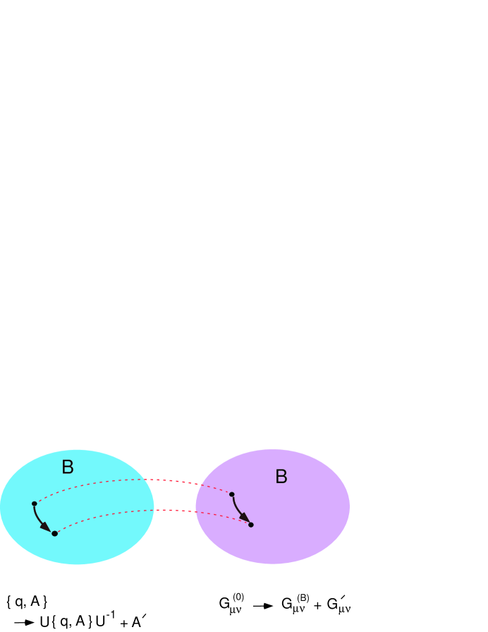
Figure 4: The muduli space of monopole-vortex configuration in the electric variables (the left figure) and in the magnetic dual variables (on the right). The points in the two $CP^{N-1}$ spaces are in one-to-one correspondence. The motion in $CP^{N-1}$ moduli space in real space-time requires the fields to be transformed nontrivially, both in the electric and magnetic descriptions.

6.1 Spacetime dependent $B$ and the effective action

Allow now the orientational moduli parameter $B$ to fluctuate in spacetime. A naïve guess is to assume

$$G_{\mu\nu}^{(0)}\to G_{\mu\nu}^{(B)}$$ (117)

also for spacetime dependent $B$ and to study the excitation of the action due to the derivatives $\partial/\partial x_{\alpha}$ acting on $\Pi_{B}$ in the kinetic term of $G_{\mu\nu}^{(B)}$, $\frac{1}{12}\hbox{\rm tr}\,(H_{\mu\nu\lambda}^{(B)})^{2},$ i.e., $H_{\mu\nu\lambda}^{(B)}\equiv\partial_{\mu}G_{\nu\lambda}^{(B)}+({\rm cyclic})$. This however is not correct.

In moving in the $CP^{N-1}$ moduli space one must make sure that the massive modes are not excited. This is the reason, in the electric description, for the introduction of the new gauge modes $A_{\alpha}$, such that the YM-matter equations of motions continue to be satisfied, i.e., to stay in the minimum-action subspace. In other words, one must stay on the minimum subsurface

$$\frac{\delta S}{\delta G_{\mu\nu}}=0$$ (118)

in all (color-flavor) directions. For $\delta G_{\mu\nu}\propto\Pi_{B}$, this is automatic; this condition must also satisfied for orthogonal fluctuations $\delta G_{\mu\nu}\propto\partial_{\alpha}\Pi_{B}$, if the system tends to generate them. Quadratic fluctuation in ${\partial_{\alpha}B}$ computed at such minimum trough then gives the correct effective action. Another equivalent way to state it is that one must maintain the correct $2D$ Nambu-Goldstone direction as the scalar and gauge fields are rotated in the color-flavor [24].

As we noted above equations of motion (113) and (114) continue to hold as long as the derivatives $\partial/\partial x_{\alpha}$ do not act on $\Pi_{B}$. Here and below we again use the indices $\alpha,\beta$ to indicate the coordinates on the worldsheet, whereas the indices $i,j$ are reserved for those in the plane perpendicular to the vortex length direction (see Fig. 3). Eq. (113) for $(\mu,\nu)=(\alpha,\beta)$ contains the equations of motion for constant $B$ (plus corrections of at least second order in the derivative of $\Pi$). Equations with $(\mu,\nu)=(i,j)$ are of higher orders in $\partial_{\alpha},\partial_{\beta}$. Potential first-order corrections are in the $(\mu,\nu)=(\beta,i)$ equation:

$$\partial_{\alpha}H^{\alpha\beta i\,(B)}+\partial_{j}H^{j\beta i\,(B)}=-m^{2}\,G^{\beta i\,(B)}$$ (119)

($\Sigma^{\mu\nu}$ term is present only for $\mu,\nu=\alpha,\beta$ (see Eq. (87)), or wrtten extensively

$$\partial^{\alpha}[\partial_{\beta}G_{i\alpha}^{(B)}+\partial_{i}G_{\alpha\beta}^{(B)}+\partial_{\alpha}G_{\beta i}^{(B)}]+\partial^{j}[\partial_{\beta}G_{ij}^{(B)}+\partial_{i}G_{j\beta}^{(B)}+\partial_{j}G_{\beta i}^{(B)}]=-m^{2}\,G_{\beta i}^{(B)}\;.$$ (120)

The gauge field for static $B$ (“unperturbed” solution with respect to $\partial_{\alpha}\Pi_{B}$) contains only

$$G_{\alpha\beta}^{(B)}=\tfrac{1}{2}\epsilon_{\alpha\beta ij}F^{(B)\,ij}=\epsilon_{\alpha\beta}\,{\cal B}^{(vor)}\Pi_{B},\qquad\epsilon_{\alpha\beta}=\begin{cases}1&\alpha\beta=03\\ -1&\alpha\beta=30\end{cases}$$ (121)

in the vortex region, far from the monopoles, where ${\cal B}_{i}=\delta_{i3}{\cal B}^{vor}$ stands for the vortex magnetic field, see Eq. (168). Eq. (120) shows that new gauge components $G^{(B)\,\beta i}$ are generated, satisfying

$$\partial^{j}[\partial_{i}G_{j\beta}^{(B)}+\partial_{j}G_{\beta i}^{(B)}]+m^{2}G_{\beta i}^{(B)}=-\partial^{\alpha}\partial_{i}G_{\alpha\beta}^{(B)}\;$$ (122)

where we have dropped terms higher order in $\partial\Pi_{B}$.

Eq. (122) can be solved for $G^{(B)\,\beta i}$ by setting

$$G_{\beta i}^{(B)}=\epsilon_{\beta i\alpha k}R^{k}\,\partial^{\alpha}\Pi_{B}\;,$$ (123)

and substituting it into Eq. (122) and recalling Eq. (121). One finds after a simple calculation that

$$R^{i}=\epsilon^{ij}\,\frac{x_{j}}{m^{2}\rho}\partial_{\rho}{\cal B}^{(vor)},\qquad\rho=\sqrt{x_{1}^{2}+x_{2}^{2}},\qquad\epsilon^{12}=-\epsilon^{21}=1\;.$$ (124)

where ${\cal B}^{(vor)}$ is the usual vortex magnetic field, Eq. (168), Eq. (169). $G^{(B)\,\beta i}$ can also be found more directly as follows. We first convert equations of motion (113) and (114) into the form,

$$\partial_{\lambda}\partial^{\lambda}G^{\mu\nu\,(B)}+m^{2}G^{\mu\nu\,(B)}=\frac{m}{\sqrt{2}e}\Sigma^{\mu\nu\,(B)}-\frac{1}{\sqrt{2}em}(\partial^{\nu}\partial_{\lambda}\Sigma^{\lambda\mu\,(B)}-\partial^{\mu}\partial_{\lambda}\Sigma^{\lambda\nu\,(B)}).$$ (125)

For a static monopole and far from the monopole, we have

$$(\partial_{i}\partial^{i}+m^{2})G^{\alpha\beta\,(B)} = \frac{m}{\sqrt{2}e}\Sigma^{\alpha\beta\,(B)}\;;$$ (126)

$$(\partial_{j}\partial^{j}+m^{2})G^{\alpha i\,(B)} = \frac{1}{\sqrt{2}em}\partial^{i}\Sigma^{\alpha\beta}\partial_{\beta}\Pi_{B}\;.$$ (127)

The solution for the first equation is

$$G^{\alpha\beta\,(B)}=\frac{m}{\sqrt{2}e}K_{0}(m\rho)\Pi_{B}$$ (128)

where $K_{0}$ is a modified Bessel function of the second kind. Solution to the second equation is then

$$G^{\alpha i\,(B)}=\frac{1}{m^{2}}\partial^{i}G^{\alpha\beta}\partial_{\beta}\Pi\;.$$ (129)

in agreement with Eqs. (123), (124).

Eq.(123) implies that the excitation energy of the vortex part is given by

$$\Delta E=f\,\hbox{\rm tr}\,(\partial_{\alpha}\Pi_{B}\partial_{\alpha}\Pi_{B}),\qquad f=\frac{2\pi}{m^{2}}\int_{0}^{\infty}d\rho\,\rho\,(\partial_{\rho}{\cal B}^{(vor)})^{2}\;.$$ (130)

The integral defining $f$ is logarithmically divergent at $\rho=0$, which must be regularized at the vortex width, $\rho\sim 1/gv_{2}$. By a simple manipulation (see e.g. [24]) this can be seen to be a $2D$ $CP^{N-1}$ action,

$$S^{2D}=2f\,\int_{\Sigma}d^{2}x\,X^{-1}\partial^{\alpha}B^{\dagger}Y^{-1}\partial_{\alpha}B\;,\qquad(X\equiv 1+B^{\dagger}B\ ,\quad Y\equiv\mathbf{1}_{N-1}+BB^{\dagger})\;,$$ (131)

defined on the worldstrip, $\Sigma$. Note that the original $4D$ integration factorized into $2+2$, because the $CP^{N-1}$ coordinate $B$ does not vary significantly over the range of the vortex width, $\sim 1/gv_{2}$.

The monopole contribution to the effective action can be found as follows. Near a pointlike monopole, $J^{0}=\tfrac{4\pi}{g}\delta^{3}({\bf r}),$ and the magnetic field $G^{0i}$ is the solution of Eq. (114):

$${\cal B}_{i}^{monopole}({\bf r})=\frac{1}{g}\,\partial_{i}\frac{e^{-gv_{2}r}}{r}\;.$$ (132)

Note that at distances larger than the vortex width, $1/gv_{2}$, this component is screened and dies out; the magnetic field $G_{0i}$ is instead dominated by the constant vortex configuration. On the other hand, near the monopole this is a standard Coulomb field. As $J^{0}$ fluctuates in time in color-flavor,

$$J^{0}\Pi\to J^{0}\Pi+{\rm const.}\,J^{0}\partial_{0}\Pi,$$ (133)

$G^{0i}$, $i=1,2,3$, acquire a component in the $\partial_{0}\Pi$ direction, around the monopole, in order to maintain Eq. (114) satisfied. It gives a singular contribution:

$$\gamma\sim\int d^{3}x\,\sum_{i=1}^{3}\,G_{0i}G^{0i}=\frac{1}{2m^{2}}\,\int d^{3}x\,\sum_{i}({\cal B}_{i}^{monopole}({\bf r}))^{2}=\frac{2\pi}{m^{2}g^{2}}\int\frac{dr}{r^{2}},$$ (134)

in the coefficient of the fluctuation amplitude, $\partial_{0}\Pi\,\partial_{0}\Pi$. The singularity is regularized at the distances $\sim 1/gv_{1}$ where the monopole turns smoothly into the regular ’t Hooft-Polyakov configuration. Therefore the integral in Eq. (134) is dominated by the radial region between $1/gv_{1}$ and $1/gv_{2}$, over which the moduli parameter $B({\bf r},t)$ is regarded as constant. The $4D$ integration here factorizes into $4=3+1$. The monopole contribution to the effective action is therefore

$$S^{1D}=\gamma\,\int_{i=M,{\bar{M}}}dt\,X^{-1}\partial_{0}B^{\dagger}({\bf r}_{i},t)Y^{-1}\partial_{0}B({\bf r}_{i},t)\;,\qquad\gamma\sim\frac{2\pi v_{1}}{g^{3}v_{2}^{2}}\sim\frac{M}{m^{2}}\;,$$ (135)

where $M=v_{1}/g$ is the monopole mass and $m=gv_{2}$ is the $W$ boson masses of the lower mass scale symmetry breaking.

The total effective action is a $2D$ $CP^{N-1}$ theory with boundaries,

$$S=S^{2D}+S_{M}^{1D}+S_{\bar{M}}^{1D}\;.$$ (136)

There is a nontrivial constraint on the variable $B(x_{\mu})$: on the boundary where the worldsheet meets the monopole worldline, the $CP^{N-1}$ variable matches:

$$B(x(\sigma,\tau))|_{\sigma=0,\pi}=B_{M,{\bar{M}}}(t(\tau))\;,$$ (137)

or

$$B(x_{3},x_{0})|_{x_{3}=x_{M\,3}}=B_{M}(x_{0})\;;\qquad B(x_{3},x_{0})|_{x_{3}=x_{M\,3}}=B_{M}(x_{0})\;.$$ (138)

This follows from Eq. (74), i.e., from the fact that the orientational zeromode of the monopole-vortex complex arises from the simultaneous $SU(N)_{C+F}$ rotations of the monopole and the light fields.

By introducing the complex unit $N$-component vector $n^{c}$ ($c=1,2,\ldots,N$):

$$n^{c}=\begin{pmatrix}X^{-\frac{1}{2}}\\ BX^{-\frac{1}{2}}\end{pmatrix}=\frac{1}{\sqrt{1+B^{\dagger}B}}\begin{pmatrix}1\\ B\end{pmatrix}\;,$$ (139)

the vortex effective action above can be put into the familiar $SU(N)$ form of the $CP^{N-1}$ sigma model,

$$S^{2D}=2f\,\int_{\Sigma}d^{2}x\,{\cal D}_{\alpha}n^{c\,\dagger}{\cal D}_{\alpha}n^{c},\qquad{\cal D}_{\alpha}n^{c}\equiv\{\partial_{\alpha}-(n^{\dagger}\partial_{\alpha}n)\}n^{c},\qquad n^{\dagger}n=1$$ (140)

and similarly for the monopole action:

$$S^{1D}=\gamma\,\int_{K=M,{\bar{M}}}dt\,{\cal D}_{0}n_{K}^{c\,\dagger}{\cal D}_{0}n_{K}^{c},$$ (141)

together with the boundary condition

$$n^{c}(x)|_{x=x_{M},x_{\bar{M}}}=n_{K}^{c}|_{K=M,{\bar{M}}}\;.\qquad$$ (142)

The boundary condition Eq. (137) or Eq. (142) can be thought of as something between Dirichlet (in the infinite monopole mass limit, $\gamma\to\infty$) and Neumann (in the light monopole limit), from the point of view of the $2D$ $CP^{N-1}$ model defined on the worldstrip of finite width .

7 Discussion

Summarizing, we have studied the vortex-monopole complex soliton configurations, in a theory with a hierarchical gauge symmetry breaking, so that the vortex ends at the monopole or antimonopole arising from the higher-mass-scale symmetry breaking. The model studied has an exact color-flavor diagonal $SU(N)_{C+F}$ symmetry unbroken in the $4D$ bulk. The individual vortex-monopole soliton breaks it, acquiring orientational $CP^{N-1}$ zeromodes. Their fluctuations are described by an effective $CP^{N-1}$ action defined on the worldstrip, the boundaries being the monopole and antimonopole worldlines; in other words, the effective action is a $2D$ $CP^{N-1}$ model with boundaries, with the boundary condition, Eq. (142), plus the monopole $1D$ $CP^{N-1}$ action. The boundary variable $n^{c}$ is a freely varying function of the worldline position, and acts as the source or sink of the excitation in the worldsheet.

This illustrates the phenomenon mentioned in the Introduction. Color fluctuation of an endpoint monopole, which in the theory without fundamental scalars suffers from the non-normalizability of the associated gauge zeromodes [17] and would remain stuck (the famous failure of the naïve nonAbelian monopole concept), escapes from the imprizonment as the color gets mixed with flavor in a color-flavor locked vacuum, and propagates freely on the vortex worldsheet. In the dual description the monopoles appear as pointlike objects, transforming under the fundamental representation of this new $SU(N)$ symmetry - the isometry group of the $CP^{N-1}$ action. It is a local $SU(N)$ symmetry, albeit in a confinement phase: these fluctuations do not propagate in the bulk outside the worldstrip. The $M-V-{\bar{M}}$ system as a whole is a singlet of the new $SU(N)$. This is appropriate because the original color $SU(N)$ is in the Higgs phase. Its dual must be in a confinement phase.

We see now how a nonAbelian dual $SU(N)$ system emerges, not plagued by any of the known problems. The so-called topological obstruction is cured here, as the bare Dirac string singularity of the monopole, which lies along the vortex core, is eaten by the vortex, so to speak. The scalar field vanishes along the vortex core, and precisely cancels the singularity in the action. This is most clearly seen in the explicit microscopic description of the monopole-vortex complex such as in [21].

Let us end with some more remarks.

Magnetic monopoles have also been studied in the context of a $U(N)$ theory in a color-flavor locked vacuum (i.e., with $N_{f}=N$ number of flavors), but without the underlying $SU(N+1)$ gauge theory [44, 45, 46, 47, 48]. By choosing unequal masses for the scalar fields, $m_{i}\neq m_{j}$ the flavor (and hence color-flavor) symmetry is explicitly broken, and degenerate $N$ Abelian vortices appear, instead of continuous set of nonAbelian vortices, parametrized by $CP^{N-1}$ moduli. Monopoles appear as kinks connecting different vortices, having masses of order of $O(|m_{i}-m_{j}|/g)$. These are Abelian monopoles. In order to find candidate nonAbelian monopoles in such a context, one must choose judiciously the scalar potential (partially degenerate) [47, 48, 49] so that one finds in the same system degenerate vortices of Abelian and nonAbelian types.

In the limit of equal masses $m_{i}=m_{j}$, the semiclassical analysis above is no longer reliable. But since in these systems the vortex is infinitely long (stable), one can make use of the facts known about the infrared dynamics of $2D$ $CP^{N-1}$ theory. It is in fact known that the quantum fluctuations of the $CP^{N-1}$ modes become strongly coupled at long distances (a $2D$ analogue of confinement) [42, 43]; it means that the vortex dynamically Abelianizes [18, 44, 45, 46]. The masses of the kink monopoles are now replaced by $O(\Lambda)$, where $\Lambda$ is the dynamical scale of the $2D$ $CP^{N-1}$ theory. In particular, in the case of an ${\cal N}=2$ supersymmetric model, the effective $2D$ theory on the vortex world sheet is a $(2,2)$ supersymmetric $CP^{N-1}$ model. Quantum effects lead to $N$ degenerate vacua ($N$ Abelian vortices); monopoles appear as kinks connecting adjacent vortices. A close connection of these objects and the $4D$ (Abelian) monopoles appearing in the infrared in $4D$, ${\cal N}=2$ supersymmetric gauge theories has been noted [44, 45, 46], which seems to realize the elegant $2D$-$4D$ duality proposal made earlier by N. Dorey [50]. These monopoles are confined by two Abelian vortices [46], in contrast to the monopoles considered in the present work.

Thus even though our system below the mass scale $v_{1}$ has some similarities as those considered in [44, 45, 46], they are clearly physically distinct. Our vortex has the endpoint monopoles, whose properties have been our main interest. In fact, the effective world sheet $CP^{N-1}$ action found here is defined on a finite worldstrip, with endpoint monopoles having their own $CP^{N-1}$ dynamics. It is an open problem what the infrared dynamics of the $CP^{N-1}$ system defined on such a finite-width worldstrip with the boundary condition Eq.(142) is, and how the low-energy phase depends on the width of the worldstrip (the vortex length).

The metastability of our vortex-monopole system also means that, when one tries to stretch the vortex it will be broken by spontaneous creation of a monopole-antimonopole pair. In this sense the vortex length itself is also a dynamical variable, dependent on the ratio $v_{2}/v_{1}$.

Another issue to be kept in mind is the possible relevance of hierarchical symmetry breaking but with reduced gauge and flavor symmetry at the first stage $v_{1}$, such as $SU(N+1)\to SU(r)\times SU(N-r)\times U(1)$. In that case the soliton vortex-monopole system carries orientational moduli of a product form, $CP^{r-1}\times CP^{N-r-1}$. It is possible that in such a system dynamical Abelianization occurs only partially [40], reminiscent of the quantum $r$ vacua of the ${\cal N}=2$ SQCD.

More generally, the monopole and antimonopole positions must also be treated as soliton collective coordinates and their motion should be taken into account as an additional piece to the action. In Eq. (141) we assumed that the monopoles are very heavy ($v_{1}\gg v_{2}$) and do not move appreciably; taking their motion into account introduces a space variable dependence of the monopole variable, $n_{K}(x_{0})\to n_{K}(x_{0},x_{3})$, $K=M,{\bar{M}}$, and the $CP^{N-1}$ dynamics and the space motion of the monopole positions will get mixed (see for example [31])).

In the large-distance approximation we have adopted, the $U(1)$ moduli of the classical ’t Hooft-Polyako monopole solutions - which rotates the exponentially damped part of the configuration [16] - is not seen. The (internal) monopole moduli ($CP^{N-1}$ rather than $CP^{N-1}\times S$) coincides with that of the vortex attached to it. Of course, the electric charge of the monopole due to Witten’s effect is correctly taken into account in our large-distance approximation, see Appendix, C.

A final remark concerns the flavor quantum numbers of the monopole, arising from e.g., the Jackiw-Rebbi effect [39]. In the case of a supersymmetric extension of the model considered here (softly-broken ${\cal N}=2$ SQCD), due to the fermion zeromodes associated with each scalar $q$ in the fundamental representaiton of $SU(N+1)$, the monopole acquires flavor global charge. Due to the normalizability of the associated fermion $3D$ zeromodes, this effect is localized near the monopole center (of distances $\sim 1/v_{1}$). Its fluctuation does not propagate, and is clearly distinct from the role played by the flavor symmetry at large distances $\sim 1/v_{2}\gg 1/v_{1}$ in generating the dual local $SU(N)$ system via the color-flavor locking. The flavor quantum number of the monopole is, in turn, fundamental in the renormalization-group behavior in the dual theory.

Global flavor symmetry thus plays several key roles, intertwined with soliton and gauge dynamics, in generating local dual nonAbelian symmetry.

Ackonowledgment

We thank Stefano Bolognesi, Simone Giacomelli, Sven Bjarke Gudnason, Muneto Nitta, Keisuke Ohashi and Norisuke Sakai for useful discussions and Keio University for hospitality.

Appendix A Minimizing the potential

The first term of Eq. (8), after going to the matrix representation of the adjoint field ($\phi\equiv\phi^{A}T^{A}$) and by using the Fierz relation (for $SU(N+1)$)

$$(T^{A})^{a}_{b}(T^{A})^{c}_{d}=-\frac{1}{2(N+1)}\delta^{a}_{b}\delta^{c}_{d}+\frac{1}{2}\delta^{a}_{d}\delta^{c}_{b},$$ (143)

reads

$$V_{\eta}=\hbox{\rm Tr}\,\left|\mu\phi-\frac{1}{2(N+1)}(\sum_{I}{q}^{\dagger\,a}_{I}q^{I}_{a}){\mathbbm{1}}+\frac{1}{2}q\,q^{\dagger}\right|^{2}\;.$$ (144)

By dropping the massive $\chi$ fields, and by using the decompositions, Eq. (16) and Eq. (37), this becomes

$${q}^{\dagger\,a}_{I}q^{I}_{a}=\eta^{\dagger}_{I}\eta_{I},\qquad q^{a}_{I}{q}^{\dagger}_{b\,I}=e^{a}_{i}\,{\bar{e}}^{j}_{b}\,\eta^{i}_{I}\eta^{\dagger}_{j\,I}\equiv e{\bar{e}}\eta\eta^{*}\;;$$ (145)

$$V_{\eta}=\hbox{\rm Tr}\left|{\mu m_{0}(N+1)}(z{\bar{z}}-\frac{1}{N+1}{\mathbbm{1}})-\frac{1}{2(N+1)}(\eta^{\dagger}_{I}\eta_{I}){\mathbbm{1}}+\frac{1}{2}e{\bar{e}}\eta\eta^{*}\right|^{2}.$$ (146)

By using the completeness

$$z{\bar{z}}+e{\bar{e}}={\mathbbm{1}},$$ (147)

$$V_{\eta} = \hbox{\rm Tr}\left|\left({\mu m_{0}N}-\frac{1}{2(N+1)}(\eta^{\dagger}_{I}\eta_{I})\right)z{\bar{z}}-\left({\mu m_{0}}+\frac{(\eta^{\dagger}_{I}\eta_{I})}{2(N+1)}\right)e{\bar{e}}+\frac{1}{2}e{\bar{e}}\eta\eta^{*}\right|^{2}.$$ (148)

$$= \left({\mu m_{0}N}-\frac{1}{2(N+1)}(\eta^{\dagger}_{I}\eta_{I})\right)^{2}+\hbox{\rm Tr}\left|\left({\mu m_{0}}+\frac{(\eta^{\dagger}_{I}\eta_{I})}{2(N+1)}\right)e{\bar{e}}-\frac{1}{2}e{\bar{e}}\eta\eta^{*}\right|^{2}$$

The minimum of the first term gives, writing

$$\eta^{\dagger}_{I}\eta_{I}\equiv N\,d^{2},$$ (149)

$$N^{2}\left({\mu m_{0}}-\frac{d^{2}}{2(N+1)}\right)=0,\qquad.^{.}.\quad d^{2}=2(N+1)\mu m_{0}\,.$$ (150)

As for the second term, one has, by using

$$\hbox{\rm Tr}(e_{i}{\bar{e}}^{i})(e_{j}{\bar{e}}^{j})=N,\qquad\hbox{\rm Tr}(e_{i}{\bar{e}}^{i})(e_{j}{\bar{e}}^{k}\eta_{I}^{j}\eta^{I\,*}_{k})=\eta^{\dagger}_{I}\eta_{I}=N\,d^{2},\qquad$$ (151)

$$\hbox{\rm Tr}(e_{j}{\bar{e}}^{k}\eta^{j}_{I}\eta^{*}_{k\,I})(e_{\ell}{\bar{e}}^{m}\eta^{\ell}_{J}\eta^{*}_{m\,J})=\delta^{k}_{\ell}\delta^{m}_{j}\eta^{j}_{I}\eta^{*}_{k\,I}\eta^{\ell}_{J}\eta^{*}_{m\,J}=(\eta^{\dagger}_{I}\eta_{J})(\eta^{\dagger}_{J}\eta_{I}),$$ (152)

and the second term of Eq. (148) becomes

$${N}\,\left[\left({\mu m_{0}}+\frac{Nd^{2}}{2(N+1)}\right)^{2}-\left({\mu m_{0}}+\frac{Nd^{2}}{2(N+1)}\right)d^{2}+\frac{d^{4}}{4}\right]=\frac{N}{2}\,\left({\mu m_{0}}-\frac{d^{2}}{2(N+1)}\right)^{2}$$ (153)

which gives the same condition as Eq. (150). Eq. (148) leads also to the conditions

$$\sum_{I\neq J}|\eta^{\dagger}_{I}\eta_{J}|^{2}=0,\quad.^{.}.\quad\eta^{\dagger}_{I}\eta_{J}=0,\quad I\neq J,\qquad\eta^{\dagger}_{1}\eta_{1}=\eta^{\dagger}_{2}\eta_{2}=\ldots=\eta^{\dagger}_{N}\eta_{N}.$$ (154)

These imply that

$$\langle\eta^{i}_{I}\rangle=\delta^{i}_{I}\,\sqrt{2(N+1)\mu m_{0}}\equiv v_{2}\,\delta^{i}_{I}\;.$$ (155)

Appendix B Monopole and vortex flux matching

The fact that the monopole magnetic flux is precisely whisked away by the vortex attached to it in the context of the hierarchical symmetry breaking, has been carefully studied by Auzzi et. al. [19], and we recall simply the results in our setting. Although the monopole is coupled to the light scalars through the field $P_{\mu}$ (see Eq. (42)), the latter is a part of the the $su(2)\subset su(N+1)$ field

$$B_{i}^{a}\frac{\tau^{a}}{2}=B_{i}^{3}\frac{\tau^{3}}{2}=\frac{1}{2g}\nabla_{i}\frac{1}{r}\left(\begin{array}[]{cc}1&0\\ 0&-1\end{array}\right)\;;$$ (156)

the magnetic flux through a tiny sphere around the monopole is given by

$$\int d{\bf S}\cdot{\bf B}=-\frac{2\pi}{g}\tau^{3}\;,\qquad\int d{\bf S}\cdot{\bf B^{3}}=-\frac{4\pi}{g}\;.$$ (157)

The vortex gauge field $A_{\mu}$ is such that the winding of the scalar field is cancelled at large distances from the vortex center, in the matter kinetic term,

$$|(\partial_{\mu}-igA_{\mu})q|^{2}\,.$$ (158)

In the gauge where the light field $\eta$ has the form, (Eq. 56), the $(11)$ component of the $SU(N)$ gauge field has the asymptotic behavior

$$A_{\phi}\sim-\frac{1}{g\rho}\;.$$ (159)

This must a part of the traceless $SU(N+1)$ gauge field

$$A_{\phi}\sim\tau^{3}\frac{1}{g\rho}\;,$$ (160)

belonging to $U(1)\subset SU(2)\subset SU(N+1)$. The vortex flux through a plane perpendicular to the vortex axis is then

$$\int d^{2}x\,\nabla\times A_{\phi}=\oint dx_{i}A^{i}=\int\rho\,d\phi\,A_{\phi}=\frac{2\pi}{g}\tau^{3}\;,$$ (161)

which matches exactly the monopole flux, Eq. (157).

Appendix C Solution of the dual equations of motion

In the presence of the static (heavy) monopoles at

$${\bf r}_{1}={\bf r}(\tau,0)=(0,0,-z_{1}),\qquad{\bf r}_{2}={\bf r}(\tau,\pi)=(0,0,0),$$ (162)

the worldstrip is at

$$\Sigma^{30}=-\Sigma^{03}=2\pi\delta(x)\delta(y)\theta(-z)\theta(z+z_{1})\;,\qquad\Sigma^{\mu\nu}=0\quad(\mu\nu)\neq(30),(03)\;;$$ (163)

which clearly satisfies the monopole confinement condition (89). The equation of motion for $G_{\mu\nu}$ has been solved in [30].

In order to interpret the result in terms of the original electric and magnetic fields, we note that the duality transformation implies ($\alpha\equiv{\theta g^{2}}/{8\pi^{2}}$):

$$F_{\mu\nu} = -\frac{m}{1+\alpha^{2}}({\tilde{G}}_{\mu\nu}-\alpha G_{\mu\nu})=-\frac{1}{g}{\tilde{\Sigma}}_{\mu\nu}-\frac{1}{m}(\partial_{\mu}L_{\nu}-\partial_{\nu}L_{\mu})\;$$ (164)

$$= -\frac{1}{g}{\tilde{\Sigma}}_{\mu\nu}-\frac{1}{\Box+m^{2}}\left[\partial_{\mu}(\alpha j_{\nu}+{\tilde{j}}_{\nu})-(\mu\leftrightarrow\nu)\right]\;.$$

For instance, let us consider a massive static monopole sitting at ${\bf r}=0$ with a vortex attached to it and extending into the $-{\hat{z}}$ direction:

$$\Sigma^{30}=-\Sigma^{03}=4\pi\,\delta(x)\delta(y)\theta(-z)\;,\qquad\Sigma^{\mu\nu}=0\quad(\mu\nu)\neq(30),(03)\;;$$ (165)

$$j^{0}=\frac{4\pi}{g}\,\delta^{3}({\bf r}),\quad j^{i}=0\;;\quad i=1,2,3\;;\qquad{\tilde{j}}^{\nu}=-\frac{1}{g}\epsilon^{\lambda\nu 03}\,\partial_{\lambda}\Sigma_{03}\;.$$ (166)

From Eq. (164) one finds that (we recall $\alpha=\theta g^{2}/8\pi^{2}$)

$${\cal E}_{i}=F_{0i}=\alpha\,{\cal B}_{i}^{(mon)},\qquad{\cal B}_{i}=\frac{1}{2}\epsilon_{ijk}F_{jk}={\cal B}_{i}^{(mon)}+{\cal B}^{(vor)}\delta_{i}^{3}\;,$$ (167)

where

$${\cal B}_{i}^{(mon)}=\frac{1}{g}\partial_{i}G({\bf r}),\qquad{\cal B}^{(vor)}=\frac{1}{g}\,m^{2}\,\int_{-\infty}^{0}\,dz^{\prime}\,G(x,y,z-z^{\prime})\;,$$ (168)

and $G({\bf r})$ is the Green function, having the Yukawa form

$$G({\bf r})=\frac{4\pi}{-\Delta+m^{2}}\,\delta^{3}({\bf r})=\frac{e^{-mr}}{r}\;.$$ (169)

Note the clear-cut separation of the monopole and vortex contributions to magnetic (and electric) fields, Eq. (167). In the vortex region, the only nonvanishing component is the magnetic field in the $x_{3}$ (vortex length) direction, $F_{12}\sim G_{03}\sim{\cal B}^{(vor)}$.

References

- [1] N. Seiberg and E. Witten, Nucl. Phys. B 426 (1994) 19; Erratum ibid. B 430 (1994) 485, [arXiv:hep-th/9407087]; N. Seiberg and E. Witten, Nucl. Phys. B 431 (1994) 484, [arXiv:hep-th/9408099].
- [2] P. C. Argyres and A. F. Faraggi, Phys. Rev. Lett 74 (1995) 3931 [arXiv:hep-th/9411047]; A. Klemm, W. Lerche, S. Theisen and S. Yankielowicz, Phys. Lett. B 344 (1995) 169 [arXiv:hep-th/9411048]; Int. J. Mod. Phys. A 11 (1996) 1929-1974 [arXiv:hep-th/9505150]; A. Hanany and Y. Oz, Nucl. Phys. B 452 (1995) 283 [arXiv:hep-th/9505075]; P. C. Argyres, M. R. Plesser and A. D. Shapere, Phys. Rev. Lett. 75 (1995) 1699 [arXiv:hep-th/9505100]; P. C. Argyres and A. D. Shapere, Nucl. Phys. B 461 (1996) 437 [arXiv:hep-th/9509175]; A. Hanany, Nucl. Phys. B 466 (1996) 85 [arXiv:hep-th/9509176].
- [3] K. Konishi and H. Terao, Nucl. Phys. B 511, 264 (1998) [arXiv:hep-th/9707005]; A. Rebhan, P. van Nieuwenhuizen, R. Wimmer, Phys. Lett. B 594, 234 (2004) [arXiv:hep-th/0307282]; Phys. Lett. B 632, 145 (2006)[arXiv:hep-th/0502221]; JHEP 0606, 056 (2006) [arXiv:hep-th/0601029].
- [4] P.C. Argyres, M.R. Plesser and N. Seiberg, Nucl. Phys. B 471, 159 (1996) [arXiv:hep-th/9603042]; P.C. Argyres, M.R. Plesser and A.D. Shapere, Nucl. Phys. B 483, 172 (1997) [arXiv:hep-th/9608129]; K. Hori, H. Ooguri and Y. Oz, Adv. Theor. Math. Phys. 1, 1 (1998) [arXiv:hep-th/9706082].
- [5] G. Carlino, K. Konishi and H. Murayama, Nucl. Phys. B 590, 37 (2000) [arXiv:hep-th/0005076].
- [6] N. Seiberg, Nucl. Phys. B 435 (1995) 129 [arXiv:hep-th/9411149]
- [7] P. C. Argyres, M. R. Plesser, N. Seiberg and E. Witten, Nucl. Phys. B 461 (1996) 71 [arXiv:hep-th/9511154].
- [8] L. Di Pietro and S. Giacomelli, JHEP 1202, 087 (2012) [arXiv:1108.6049 [hep-th]].
- [9] T. Eguchi, K. Hori, K. Ito and S.-K. Yang, Nucl. Phys. B 471 (1996) 430 [arXiv:hep-th/9603002].
- [10] G. Carlino, K. Konishi, S. P. Kumar and H. Murayama, Nucl. Phys. B 608, 51 (2001) [arXiv:hep-th/0104064].
- [11] S. Giacomelli and K. Konishi, JHEP 1303, 009 (2013) [arXiv:1301.0420 [hep-th]]; S. Giacomelli and K. Konishi, JHEP 1303, 009 (2013) [arXiv:1301.0420 [hep-th]].
- [12] P. C. Argyres and N. Seiberg, JHEP 0712, 088 (2007) [arXiv:0711.0054 [hep-th]].
- [13] D. Gaiotto, N. Seiberg and Y. Tachikawa, JHEP 1101, 078 (2011) [arXiv:1011.4568 [hep-th]].
- [14] S. Giacomelli, JHEP 1209, 040 (2012) [arXiv:1207.4037 [hep-th]].
- [15] A. Abouelsaood, Nucl. Phys. B 226, 309 (1983); P. Nelson, A. Manohar, Phys. Rev. Lett. 50, 943 (1983); A. Balachandran, G. Marmo, M. Mukunda, J. Nilsson, E. Sudarshan, F. Zaccaria, Phys. Rev. Lett. 50, 1553 (1983); P. Nelson, S. Coleman, Nucl. Phys. B 227, 1 (1984).
- [16] E. J. Weinberg, Nucl. Phys. B 167, 500 (1980); Nucl. Phys. B 203, 445 (1982); K. Lee, E. J. Weinberg, P. Yi, Phys. Rev. D 54 , 6351 (1996)
- [17] N. Dorey, C. Fraser, T.J. Hollowood, M.A.C. Kneipp, Phys. Lett. B 383, 422 (1996) [arXiv: hep-th/9512116].
- [18] R. Auzzi, S. Bolognesi, J. Evslin, K. Konishi and A. Yung, Nucl. Phys. B 673 (2003) 187 [arXiv:hep-th/0307287].
- [19] R. Auzzi, S. Bolognesi, J. Evslin and K. Konishi, Nucl. Phys. B 686 (2004) 119 [arXiv:hep-th/0312233]; M.A.C. Kneipp, Phys. Rev. D 69: 045007 (2004) [arXiv:hep-th/0308086].
- [20] M. Eto, L. Ferretti, K. Konishi, G. Marmorini, M. Nitta, K. Ohashi, W. Vinci and N. Yokoi, Nucl. Phys. B 780 161-187, 2007 [arXiv:hep-th/0611313].
- [21] M. Cipriani, D. Dorigoni, S. B. Gudnason, K. Konishi and A. Michelini, Phys. Rev. D 84, 045024 (2011) [arXiv:1106.4214 [hep-th]].
- [22] K. Konishi, in Lecture Notes in Physics, 737 471 (2008), Springer [arXiv:hep-th/0702102].
- [23] L. Ferretti, S. B. Gudnason and K. Konishi, Nucl. Phys. B 789, 84 (2008) [arXiv:0706.3854 [hep-th]], S. B. Gudnason and K. Konishi, Phys. Rev. D 81, 105007 (2010) [arXiv:1002.0850 [hep-th]].
- [24] S. B. Gudnason, Y. Jiang and K. Konishi, JHEP 1008:012 (2010) [arXiv:007.2116 [hep-th]].
- [25] A. Hanany and D. Tong, JHEP 0307 (2003) 037 [arXiv:hep-th/0306150].
- [26] J. Evslin, S. Giacomelli, K. Konishi and A. Michelini, JHEP 1106 (2011) 094 [arXiv:1103.5969 [hep-th]].
- [27] Y. M. Cho, Phys. Rev. D 21 (1980) 1080.
- [28] K. Seo, M. Okawa and A. Sugamoto, Phys. Rev. D 19, 3744 (1979) ; Y. Hirono, T. Kanazawa and M. Nitta, Phys. Rev. D 83, 085018 (2011) [arXiv:1012.6042 [hep-ph]].
- [29] C. Chatterjee and A. Lahiri, JHEP 1002, 033 (2010) [arXiv:0912.2168 [hep-th]].
- [30] K. Konishi, A. Michelini and K. Ohashi, Phys. Rev. D 82, 125028 (2010) [arXiv:1009.2042 [hep-th]].
- [31] M. Cipriani and T. Fujimori, [arXiv:1207.2070 [hep-th]].
- [32] F. Delduc and G. Valent, Nucl. Phys. B 253, 494 (1985); F. Delduc and G. Valent, Phys. Lett. B 148 (1984) 124.
- [33] K. -M. Lee, Phys. Rev. D 48, 2493 (1993) [arXiv:hep-th/9301102].
- [34] K. Ohashi, unpublished.
- [35] R. Auzzi, M. Eto and W. Vinci, JHEP 0711:090 (2007) [arXiv:0709.1910 [hep-th]].
- [36] Y. Nambu, Phys. Rev. D 10, 4262 (1974).
- [37] E. T. Akhmedov, M. N. Chernodub, M. I. Polikarpov and M. A. Zubkov, Phys. Rev. D 53, 2087 (1996) [arXiv:hep-th/9505070].
- [38] A. Milekhin, Phys. Rev. D 86, 105002 (2012) [arXiv:1207.0417 [hep-th]].
- [39] R. Jackiw, C. Rebbi, Phys. Rev. D 13, 3398 (1976).
- [40] D. Dorigoni, K. Konishi and K. Ohashi, Phys. Rev. D 9 (2009) 045011 [arXiv:0801.3284 [hep-th]].
- [41] N. Manton, Phys. Lett. B 154, 397 (1985), Erratum-ibid. B 157, 475 (1985).
- [42] E. Witten, Nucl. Phys. B 149, 285 (1979).
- [43] V. A. Novikov, M. A. Shifman, A. I. Vainshtein and V. I. Zakharov, Phys. Rept. 116, 103 (1984) [Sov. J. Part. Nucl. 17, 204 (1986)] [Fiz. Elem. Chast. Atom. Yadra 17, 472 (1986)].
- [44] M. Shifman, A. Yung, Phys. Rev. D70, 045004 (2004). [arXiv: hep-th/0403149].
- [45] A. Hanany and D. Tong, JHEP 0404, 066 (2004) [arXiv: hep-th/0403158].
- [46] A. Gorsky, M. Shifman, A. Yung, Phys. Rev. D 71, 045010 (2005) [arXiv: hep-th/0412082].
- [47] M. Nitta and W. Vinci, Nucl. Phys. B 848, 121 (2011) [arXiv:1012.4057 [hep-th]].
- [48] M. Eto, T. Fujimori, S. B. Gudnason, Y. Jiang, K. Konishi, M. Nitta and K. Ohashi, JHEP 1112, 017 (2011) [arXiv:1108.6124 [hep-th]].
- [49] S. Monin and M. Shifman, Int. J. Mod. Phys. A 29, no. 18, 1450105 (2014) [arXiv:1309.4527 [hep-th]].
- [50] N. Dorey, JHEP 9811, 005 (1998) [hep-th/9806056].