The quark induced Mueller-Tang jet impact factor at next-to-leading order

Abstract

We present the NLO corrections for the quark induced forward production of a jet with an associated rapidity gap. We make use of Lipatov’s QCD high energy effective action to calculate the real emission contributions to the so-called Mueller-Tang impact factor. We combine them with the previously calculated virtual corrections and verify ultraviolet and collinear finiteness of the final result.

1 Introduction

A very interesting test of QCD in the high energy limit is provided by dijet events with associated rapidity gaps. As originally pointed out by Mueller and Tang [1], this type of events, when the tagged jets are far apart in rapidity, allow for the study of the Balitsky-Fadin-Kuraev-Lipatov (BFKL) hard pomeron [2] at finite momentum transfer $t\neq 0$. Absence of hadronic activity over a large region in rapidity $\Delta y_{\text{gap}}$ suggests that an important contribution to the dijet cross-section is due to configurations with color singlet exchange in the $t$-channel. Such exchange is well described by the non-forward BFKL Green’s function with finite momentum transfer. Unlike the case of zero momentum transfer, which describes the rise of total cross-sections and has been investigated for a number of observables (see e.g. [3, 4, 5]) the BFKL dynamics with finite momentum transfer remains relatively unexplored.

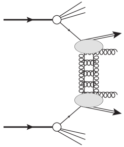
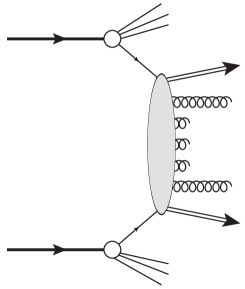
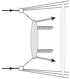
(a)

(b)

(c)

Figure 1: Contributions to the Mueller-Tang cross-section: a) color singlet exchange; b) emissions with $p_{T}$ smaller than the experimental resolution in the rapidity gap; c) soft rescattering of the hadron remnants which destroy the rapidity gap.

While dijets with associated rapidity gaps allow to access such dynamics, precise phenomenology remains a challenging task.

The configurations of interest with color singlet exchange, Fig. 1.a, which do not generate any emission into the gap, compete with color exchange contributions where emissions are allowed up to a scale set by the experimental resolution $E_{\text{gap}}$ of the rapidity gap definition, Fig. 1.b. Moreover jet-gap-jet events are affected by soft rescatterings of the proton remnants which destroy the rapidity gap and lead to a violation of collinear factorization, see Fig. 1.c; for further details we refer to [6] and references therein.

In this work we study the color singlet $t$-channel exchange contribution within the framework of high energy factorization. A complete description is currently only available at leading logarithmic (LL) accuracy, where terms enhanced by the gap size $(\alpha_{s}\Delta y_{\text{gap}})^{n}$ are resummed to all orders in the strong coupling $\alpha_{s}$. Phenomenological studies, including a comparison to data by the D0 and CDF collaboration at Tevatron/Fermilab have been performed in [7, 8] and later on by [9], where a subset of the NLO corrections was included. Given the importance of the NLO corrections to both impact factors and Green’s function found in the forward limit, a similar study in the non-forward case is mandatory. High precision in the calculations is even more pressing since the BFKL driven color singlet exchange needs to be isolated from other competing contributions. In particular, the study of the possible effects due to non-perturbative gap survival probability factors, makes an accurate description of the perturbative sub-process crucial for the correct understanding of the diffractive observables. While the NLO non-forward BFKL kernel is well known [10], both in momentum and configuration space [11], the NLO corrections for the impact factors are only available at the level of virtual corrections i.e. for elastic parton-parton scattering amplitudes [12, 13].

Here we calculate the NLO impact factors for quark induced jets with color singlet exchange using Lipatov’s effective action [14]. The determination of the gluon induced jets will be addressed in a follow-up paper [15]. The calculation of higher order corrections from the effective action approach [14] has been successfully explored by our group in recent years. In particular, both NLO impact factors for quark [16] and gluon induced forward jets [17] and the gluon Regge trajectory up to two loops [18] have been obtained making use of Lipatov’s effective action and a set of supplementary calculational rules. In the following we will use this framework for the determination of the missing real NLO corrections which will be then combined at partonic level with the already known virtual corrections. Introducing a jet definition and integrating over the real emission phase space, we finally verify that all remaining singularities are removed by renormalization of the QCD Lagrangian and collinear factorization. While, in general, infrared finiteness is to be expected, it presents an important result in the present context, given the notoriously complicated perturbative QCD environment for jet-gap-jet events.

The outline is as follows: Sec. 2 provides a definition of the NLO Mueller-Tang jet impact factor and Sec. 3 contains a short review of the high energy effective action. In Sec. 4 we give some details on the derivation of the leading order Mueller-Tang impact factor and the real next-to-leading order corrections from the effective action. Sec. 5 addresses the definition of the quark induced Mueller-Tang jet vertex at NLO within collinear factorization. In Sec. 6 we summarize our results, already presented in [19], and provide an outlook for future work. Two appendices gather additional material concerning the high energy limit of the NLO impact factor (Appendix A) and explicit results for the inclusive (perturbative) Pomeron - quark impact factor (Appendix B).

2 The NLO Mueller-Tang impact factor - definition

We are interested in the hadron-hadron scattering process

$$h(p_{A})+h(p_{B})\to J_{1}(p_{J,1})+J_{2}(p_{J,2})+\text{gap},$$ (1)

with two jets produced in the final state separated by a large rapidity gap, which is characterized by no hadronic activity in the detectors. In addition we limit ourselves to color singlet exchange in the the $t$-channel. As outlined in the introduction, the latter constraint is at first a theoretical one and it remains a task for future phenomenological analysis to determine those observabels for which this configuration is dominant. For an interesting proposal in this direction see [20].

With quark exchange in the $t$-channel suppressed by a factor $\sim\exp(-\Delta y_{\text{gap}})$, color singlet exchange appears for large $\Delta y_{\text{gap}}$ for the first time at $\mathcal{O}(\alpha_{s}^{4})$. It constitutes therefore a NNLO correction, relative to the conventional dijet cross-section. While this is beyond the reach of current exact calculations, the presence of a large rapidity gap suggests that a description of this process in terms of high energy factorized amplitudes can provide a good approximation to the full result. To this end we define light-cone vectors as rescaled light-like momenta of the incoming hadrons $n^{\pm}=2p_{A,B}/\sqrt{s}$ with $s=2p_{A}\cdot p_{B}$. Assuming massless jets, the Sudakov decomposition of the external particle momenta reads

$$p_{A} =p_{A}^{+}\frac{n^{-}}{2}, p_{J,1} =\sqrt{{\bm{k}}_{J,1}^{2}}\left(e^{y_{J,1}}\frac{n^{-}}{2}+e^{-y_{J,1}}\frac{n^{+}}{2}\right)+{\bm{k}}_{J,1};$$

$$p_{B} =p_{B}^{-}\frac{n^{+}}{2}, p_{J,2} =\sqrt{{\bm{k}}_{J,2}^{2}}\left(e^{y_{J,2}}\frac{n^{-}}{2}+e^{-y_{J,2}}\frac{n^{+}}{2}\right)+{\bm{k}}_{J,2};$$ (2)

with $({\bm{k}}_{J,i},y_{J,i})$, $i=1,2$ being the transverse momenta and rapidity of the jet. To obtain the hadronic dijet cross-section, we first calculate the corresponding partonic cross-sections. For quark induced jets we need the leading order (LO) high energy limit of the process

$$q(p_{a})+q(p_{b})\to q(p_{1})+q(p_{2}),$$ (3)

with color singlet exchange in the $t$-channel. In the high energy limit $\hat{s}\to\infty$ with $\hat{s}=2p_{a}\cdot p_{b}$ and in $d=4+2\epsilon$ dimensions, the partonic cross-section, rederived in Sec. 4.1, reads

$$d\hat{\sigma}_{ab} =h_{q,a}^{(0)}h_{q,b}^{(0)}\left[\int\frac{d^{2+2\epsilon}{\bm{l}}_{1}}{\pi^{1+\epsilon}}\frac{1}{{\bm{l}}_{1}^{2}({\bm{k}}-{\bm{l}}_{1})^{2}}\right]\left[\int\frac{d^{2+2\epsilon}{\bm{l}}_{2}}{\pi^{1+\epsilon}}\frac{1}{{\bm{l}}_{2}^{2}({\bm{k}}-{\bm{l}}_{2})^{2}}\right]d^{2+2\epsilon}{\bm{k}}\,.$$ (4)

Here $h_{q}^{(0)}$ denotes the LO impact factor. Resummation of $\Delta y_{\text{g}ap}$ enhanced terms to all orders in the strong coupling $\alpha_{s}$ is then achieved through replacing the transverse gluon propagators with the non-forward BFKL Green’s function $G({\bm{l}},{\bm{l}}^{\prime},{\bm{q}},s/s_{0})$, where the latter is obtained as a solution to the non-forward BFKL equation.

The resummed cross-section takes the form

$$d\hat{\sigma}_{ab}^{\text{res.}} =h_{q,a}^{{(0)}}h_{q,b}^{{(0)}}\left[\int\frac{d^{2+2\epsilon}{\bm{l}}_{1}}{{\pi}^{1+\epsilon}}\int\frac{d^{2+2\epsilon}{\bm{l}}_{1}^{\prime}}{{\pi}^{1+\epsilon}}G\left({\bm{l}}_{1},{\bm{l}}_{1}^{\prime},{\bm{k}},\frac{\hat{s}}{s_{0}}\right)\right]$$

$$\qquad\qquad\qquad\qquad\left[\int\frac{d^{2+2\epsilon}{\bm{l}}_{2}}{\pi^{1+\epsilon}}\int\frac{d^{2+2\epsilon}{\bm{l}}^{\prime}_{2}}{\pi^{1+\epsilon}}G\left({\bm{l}}_{2},{\bm{l}}_{2}^{\prime},{\bm{k}},\frac{\hat{s}}{s_{0}}\right)\right]d^{2+2\epsilon}{\bm{k}}.$$ (5)

In this expression $s_{0}$ denotes the reggeization scale, which parametrizes the scale uncertainty due to the all order resummation. Constraining the $s_{0}$ dependence is an additional benefit of a complete NLO treatment while the natural choice for $s_{0}$ is $\ln(\hat{s}/s_{0})=\Delta y_{\text{gap}}$. Apparently both transverse integrals in Eq. (29) are divergent and a suitable infrared regulator is needed. This divergence is in principle also present in the (LO) Green’s function. However, in the asymptotic limit $\ln(\hat{s}/s_{0})\to\infty$, the dependence on the infrared regulator vanishes and the result turns out to be finite [8]. The combination with an approach resumming logarithms in the jet transverse momentum and the gap resolution $E_{\text{gap}}$, including a matching of singularities at finite perturbative orders of the BFKL Green’s function has been discussed in [22]. In the following we assume that these singularities are addressed in a suitable way, either through a suitable matching and/or by working in the strict asymptotic limit $\ln(\hat{s}/s_{0})\to\infty$. In particular, the integrals over transverse momentum are assumed to yield a finite result.

To calculate the NLO impact factors it is needed to determine both the 1-loop corrections to the process (3) and the leading order process

$$q(p_{a})+q(p_{b})\to q(p_{1})+q(p_{2})+g(q),$$ (6)

with color singlet exchange in one of the $t$-channels $t_{1}=(p_{a}-p_{1})^{2}$ and $t_{2}=(p_{b}-p_{2})^{2}$. The 1-loop corrections to Eq. (3) have been obtained in [12]. As the non-forward BFKL Green’s function generates no real emissions, the entire $s_{0}$ dependence is for this particular process contained in the virtual corrections to the impact factors. As verified in [12], the $s_{0}$ dependence cancels if the all-order Green’s function is truncated at NLO.

Both at LO and NLO, it is necessary to restrict the phase space of the final state system, to avoid particle emissions into the forbidden gap region. To be more precise, we will require that the invariant mass of the diffractive system in the forward region of each proton to be smaller than a certain upper cut-off $M_{X,\text{max}}^{2}$, set by experiment. At LO, contributions to the diffractive system are due to initial state radiation, which is encoded in the parton distribution functions, while at NLO this includes also contributions from the produced partonic system. For the diffractive system in the forward region of the proton with momentum $p_{A}$ we find (the $t$-channel momentum is $k=p_{b}-p_{2}$) at partonic level:

$$\hat{M}_{X}^{2} =(p_{a}+k)^{2}=p_{a}^{+}k^{-}-{\bm{k}}^{2}\;.$$ (7)

At LO $\hat{M}_{X}^{2}=0$, while $\hat{M}_{X}^{2}$ assumes a finite value at NLO. It is related to the diffractive mass at hadronic level through

$$\hat{M}_{X}^{2} =x_{1}M_{X}^{2}-(1-x_{1}){\bm{k}}^{2}\;.$$ (8)

The constraint $M_{X}^{2}<M_{X,\text{max}}^{2}$ leads then to the following lower bound on the proton momentum fraction of the incoming parton

$$x_{1}>x_{0}=\frac{{\bm{k}}^{2}}{M_{X,\text{max}}^{2}+{\bm{k}}^{2}}\;,$$ (9)

while at NLO, in addition, the phase space of the partonic quark-gluon final state system is constrained.

To obtain the dijet cross-section from the partonic process, we further require a function which selects the configurations contributing to the particular choice of jet definition made in an experiment from the full partonic final state phase space. Formally, this is achieved through the convolution with a distribution $S_{J}$, which contains the details about the chosen jet algorithm. Schematically, the partonic differential cross-section reads

$$\frac{d\hat{\sigma}_{J}}{dJ_{1}dJ_{2}d^{2}{\bm{k}}} =\,{d\hat{\sigma}}\,\otimes\,S_{J_{1}}S_{J_{2}}\,\,\;,$$ (10)

with $dJ_{i}=d^{2}{\bm{p}}_{J_{i}}dy_{J_{i}}$ the jet phase space and ${\bm{k}}$ the $t$-channel transverse momentum transfer. At leading order, ${\bm{k}}$ coincides with the transverse momentum of the jet and the jet functions are trivial. They map each of the final state quarks with one of the jets through

$$S^{(2)}_{J_{i}}({\bm{p}}_{i},x_{i}) =x_{i}\,\delta\left(x_{i}-\frac{|{\bm{k}}_{J,i}|{e^{y_{J,i}}}}{\sqrt{s}}\right)\delta^{2+2\epsilon}({\bm{p}}_{i}-{\bm{k}}_{J_{i}}), i =1,2\;.$$ (11)

In particular, due to the large rapidity gap spanned between the two jets, the quark with momentum $p_{i}$ corresponds directly to the jet with momentum $p_{J,i}$, $i=1,2$. The full NLO treatment will be addressed in Sec. 5. We stress that in addition to the phase space of the two jets, the cross-section Eq. (10) is also differential in the (transverse) momentum transfer through the gap region. As long as LO impact factors are used, the cross-section describes essentially elastic quark-quark scattering and this momentum transfer is identical to the transverse jet momentum. As soon as the diffractive system contains other objects than the jet, scattering is no longer elastic and both transverse momenta deviate. In principle, this quantity is measurable as the total transverse momentum of the diffractive systems. In practical applications, the cross-section of Eq. (10) is probably too differential and one would prefer to integrate over some of the variables. A possibility is to make the deviation from purely elastic scattering explicit through the following parametrization of the jet transverse momenta

$${\bm{k}}_{J,1} ={\bm{p}}+\Delta{\bm{p}}, {\bm{k}}_{J,2} =-{\bm{p}}+\Delta{\bm{p}},$$ (12)

and to integrate both over $\Delta{\bm{p}}$ and ${\bm{k}}$ as well as the overall rapidity $y=y_{1}+y_{2}$, resulting into a cross-section differential in the mean transverse momentum $2{\bm{p}}={\bm{k}}_{J,1}-{\bm{k}}_{J,2}$ and the rapidity difference of the two jets. Here we focus on the determination of impact factors and leave such details concerning the construction of suitable observables out of the (maximal) differential cross-section as a task for a future phenomenological studies.

To the end of describing the full hadronic process of Eq. (1) we convolute the partonic process in Eq. (10) with parton distribution functions. In principle, the use of collinear factorization can be questioned for this type of processes since soft re-scattering of the hadron remnants can destroy the rapidity gap and lead to its violation. At partonic level, violation of factorization is manifest through the divergent transverse integrals in Eq. (29) at finite $\ln\hat{s}/s_{0}$. In the following we use the working assumption that all initial state collinear singularities of the impact factors can be consistently absorbed through the conventional redefinition of the parton distribution functions. We will demonstrate in Sec. 5 that this is actually the case and that the impact factor itself is a well-defined quantity. The final cross-section then takes the following form

$$\frac{d\sigma}{dJ_{1}\,dJ_{2}\,\,d^{2}{\bm{k}}} =\sum_{l,k=q,\bar{q}}\int_{0}^{1}dx_{1}\,\int_{0}^{1}dx_{2}\,\,f_{l/p}^{\text{gap}}(x_{1},\mu_{f})\,\,f_{k/p}^{\text{gap}}(x_{2},\mu_{f})\,\,H_{kl}(x_{1},x_{2},\mu_{f}),$$ (13)

where we suppressed for the collinear coefficient $H_{kl}$ the dependence on the final state variables. At LO, $H_{qq}$ coincides with the partonic cross-section in Eq. (10), while the NLO treatment requires at first the identification of initial state collinear singularities. Furthermore, we added to each of the (anti-) quark distribution functions the superscript ‘gap’. This is meant to indicate that these distributions do not necessarily coincide with standard pdfs. In phenomenological applications they may be calculated from the standard pdfs using phenomenological gap survival probability factors and/or restricting to certain combinations of observables which are insensitive to possible soft rescatterings, see e.g. [20].

3 The High-Energy Effective Action

For the calculation of the missing real NLO corrections, we make use of Lipatov’s high energy effective action [14]. Within this framework, QCD amplitudes are in the high energy limit decomposed into gauge invariant sub-amplitudes which are localized in rapidity space and describe the coupling of quarks ($\psi$), gluon ($v_{\mu}$) and ghost ($\phi$) fields to a new degree of freedom, the reggeized gluon field $A_{\pm}(x)$. The latter is introduced as a convenient tool to reconstruct the complete QCD amplitudes in the high energy limit out of the sub-amplitudes restricted to small rapidity intervals.

Lipatov’s effective action is obtained by adding an induced term $S_{\text{ind.}}$ to the QCD action $S_{\text{QCD}}$,

$$S_{\text{eff}} =S_{\text{QCD}}+S_{\text{ind.}}\;,$$ (14)

where the induced term $S_{\text{ind.}}$ describes the coupling of the gluonic field $v_{\mu}=-it^{a}v_{\mu}^{a}(x)$ to the reggeized gluon field $A_{\pm}(x)=-it^{a}A_{\pm}^{a}(x)$. High energy factorized amplitudes reveal strong ordering in plus and minus components of momenta which is reflected in the following kinematic constraint obeyed by the reggeized gluon field:

$$\partial_{+}A_{-}(x) =0=\partial_{-}A_{+}(x).$$ (15)

Even though the reggeized gluon field is charged under the QCD gauge group SU$(N_{c})$, it is invariant under local gauge transformation $\delta A_{\pm}=0$. Its kinetic term and the gauge invariant coupling to the QCD gluon field are contained in the induced term

$$S_{\text{ind.}}=\int\text{d}^{4}x\,\text{tr}\left[\left(W_{-}[v(x)]-A_{-}(x)\right)\partial^{2}_{\perp}A_{+}(x)\right]+\text{tr}\left[\left(W_{+}[v(x)]-A_{+}(x)\right)\partial^{2}_{\perp}A_{-}(x)\right],$$ (16)

with

$$W_{\pm}[v(x)]= v_{\pm}(x)\frac{1}{D_{\pm}}\partial_{\pm}, D_{\pm} =\partial_{\pm}+gv_{\pm}(x).$$ (17)

For a more in depth discussion of the effective action we refer to the recent review [21]. Due to the induced term in Eq. (14), the Feynman rules of the effective action comprise, apart from the usual QCD Feynman rules, the propagator of the reggeized gluon and an infinite number of so-called induced vertices. Vertices and propagators needed for the current study are collected in Fig. 2.

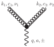
$=\displaystyle\begin{array}[h]{ll}\\ \\ -i{\bm{q}}^{2}\delta^{ac}(n^{\pm})^{\nu},\\ \\ \qquad k^{\pm}=0.\end{array}$ $=\displaystyle\begin{array}[h]{ll}\delta^{ab}\frac{i/2}{{\bm{q}}^{2}}\end{array}$ $\displaystyle=\begin{array}[h]{ll}\\ \\ gf^{c_{1}c_{2}a}\frac{{\bm{q}}^{2}}{k_{1}^{\pm}}(n^{\pm})^{\nu_{1}}(n^{\pm})^{\nu_{2}},\\ \\ \quad k_{1}^{\pm}+k_{2}^{\pm}=0\end{array}$
(a) (b) (c)

Figure 2: Feynman rules for the lowest-order effective vertices of the effective action. Wavy lines denote reggeized fields and curly lines gluons.

Determination of NLO corrections using this effective action approach has been addressed recently to a certain extent, through the explicit calculation of the NLO corrections to both quark [16] and gluon [17] induced forward jets (with associated radiation) as well as the determination of the gluon Regge trajectory up to 2-loops [18]. These previous applications have all in common that they are, at amplitude level, restricted to a color octet projection and, therefore, single reggeized gluon exchange. Due to the particular color structure of the reggeized gluon field, which is restricted to the anti-symmetric color octet, see Fig. 2 and [14, 26], color singlet exchange requires to go beyond a single reggeized gluon exchange and to consider the two reggeized gluon exchange contribution.

4 The high energy factorized cross-section at partonic level

4.1 The Mueller-Tang jet cross-section at LO

$=$ +

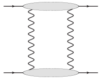
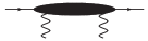
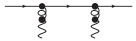
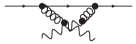
(a)

(b)

Figure 3: a) The LO amplitude for quark induced jets in the high energy approximation. The 2 reggeized gluon state in the $t$-channel is projected on the color singlet. b) LO diagrams which describe within the effective action the coupling of the two-reggeized gluon state to the quark.

The Mueller-Tang jet impact factor at leading order can be determined from the elastic scattering amplitude $q(p_{a})+q(p_{b})\to q(p_{1})+q(p_{2})$ with color singlet exchange. In the high energy limit, such a color singlet exchange is within the effective action – to LO in the strong coupling $\alpha_{s}$ – provided by the $t$-channel exchange of two reggeized gluons in the color singlet state, Fig. 3.b. With the Sudakov decomposition of the external momenta,

$$p_{a} =p_{a}^{+}\frac{n^{-}}{2} p_{1} =p_{a}^{+}\frac{n^{-}}{2}+k^{-}\frac{n^{+}}{2}+{\bm{k}}$$

$$p_{b} =p_{b}^{-}\frac{n^{+}}{2} p_{2} =p_{b}^{-}\frac{n^{+}}{2}-k^{+}\frac{n^{-}}{2}-{\bm{k}},$$ (18)

where the kinematic constraint, Eq. (15), has been taken into account, the Mandelstam invariants read

$$s =p_{a}^{+}p_{b}^{-} t=-{\bm{k}}^{2}\;,$$ (19)

and the quark-quark scattering amplitude with color singlet exchange is at leading order given by

$$i\mathcal{M}=\frac{1}{2\cdot 2!}\int\frac{dl^{+}dl^{-}}{(2\pi)^{2}}\int\frac{d^{2+2\epsilon}{\bm{l}}}{(2\pi)^{2+2\epsilon}}i\tilde{\mathcal{M}}^{de}_{q2r_{+}^{*}\to q}P^{de}\cdot i\tilde{\mathcal{M}}^{d^{\prime}e^{\prime}}_{q2r_{-}^{*}\to q}P^{d^{\prime}e^{\prime}}\frac{(i/2)^{2}}{{\bm{l}}^{2}({\bm{l}}-{\bm{k}})^{2}}\;,$$ (20)

with

$$\mathcal{P}^{ab,a^{\prime}b^{\prime}} =P^{ab}P^{a^{\prime}b^{\prime}}, P^{ab} =\frac{\delta^{ab}}{\sqrt{N_{c}^{2}-1}},$$ (21)

being the projector onto the color singlet. The Sudakov decomposition of the momenta of the sub-process $q(p_{a})+r_{+}^{*}(l_{1})+r_{+}^{*}(k-l_{1})\to q(p)$ reads

$$p_{a} =p_{a}^{+}\frac{n^{-}}{2} p =p_{a}^{+}\frac{n^{-}}{2}+k^{-}\frac{n^{+}}{2}+{\bm{k}}$$

$$l_{1} =l_{1}^{-}\frac{n^{+}}{2}+{\bm{l}}_{1} k =k^{-}\frac{n^{+}}{2}+{\bm{k}},$$ (22)

with

$$i\tilde{\mathcal{M}}^{ed}_{q2r_{+}^{*}\to q}\mathcal{P}^{ed} =-g^{2}\bar{u}(p)\text{$n$$\diagup$\hskip 3.00117pt}^{+}u(p_{a})\frac{\delta_{i_{1}i_{a}}C_{F}}{\sqrt{N_{c}^{2}-1}}\cdot\bigg{[}\frac{2i}{l^{-}-\frac{{\bm{l}}^{2}-i\epsilon}{p_{a}^{+}}}+\frac{2i}{k^{-}-l^{-}-\frac{({\bm{k}}-{\bm{l}})^{2}-i\epsilon}{p_{a}^{+}}}\bigg{]}.$$ (23)

Due to Eq. (15), the entire dependence on the longitudinal loop momenta $l^{-}$ and $l^{+}$ is contained in the $qr^{*}r^{*}\to q$ amplitudes. Note that this observation holds also for the case where higher order corrections to the $qr^{*}r^{*}\to q$ amplitude are included and/or there are additional particles in the final state. Due to this property it is possible to express Eq. (20) as a transverse loop integral alone,

$$i\mathcal{M}=\int\frac{d^{2+2\epsilon}{\bm{l}}}{(2\pi)^{2+2\epsilon}}\phi_{qq,a}\phi_{qq,b}\frac{1}{{\bm{l}}^{2}({\bm{l}}-{\bm{k}})^{2}},$$ (24)

with

$${i}\phi_{qq} =\int\frac{dl^{-}}{8\pi}i\tilde{\mathcal{M}}^{ab}_{qr^{*}r^{*}\to q}P^{ab}=-\delta_{i_{1}i_{a}}\frac{g^{2}}{4}\frac{C_{f}}{\sqrt{N_{c}^{2}-1}}\bar{u}_{(\lambda)}(p)\text{$n$$\diagup$\hskip 3.00117pt}^{+}u_{(\lambda)}(p_{a}).$$ (25)

For later use we also give the result for the leading order gluon impact factor

$$i\phi_{gg}=\delta_{c_{1}c_{a}}{g^{2}}\frac{C_{a}}{\sqrt{N_{c}^{2}-1}}p_{a}^{+}{\bm{\epsilon}}_{(\lambda)}^{*}(p)\cdot{\bm{\epsilon}}_{(\lambda)}(p_{a}),$$ (26)

where gluon polarization vectors in the ‘right-handed light cone gauge’ have been used. The latter obey the conditions

$$\epsilon_{(\lambda)}(p,n^{+})\cdot p =0 \epsilon_{(\lambda)}(p,n^{+})\cdot n^{+} =0,$$ (27)

and can be parametrized as

$$\epsilon^{\mu}_{(\lambda)}(p,n^{+}) =\frac{{\bm{\epsilon}}_{(\lambda)}\cdot{\bm{p}}}{p^{+}}(n^{+})^{\mu}+{\bm{\epsilon}}_{(\lambda)}^{\mu}.$$ (28)

Using these results, we obtain the LO partonic differential cross-section for dijets with color singlet exchange as

$$d\hat{\sigma}_{ab} =h_{q,a}^{(0)}h_{q,b}^{(0)}\left[\int\frac{d^{2+2\epsilon}{\bm{l}}_{1}}{\pi^{1+\epsilon}}\frac{1}{{\bm{l}}_{1}^{2}({\bm{k}}-{\bm{l}}_{1})^{2}}\right]\left[\int\frac{d^{2+2\epsilon}{\bm{l}}_{2}}{\pi^{1+\epsilon}}\frac{1}{{\bm{l}}_{2}^{2}({\bm{k}}-{\bm{l}}_{2})^{2}}\right]d^{2+2\epsilon}{\bm{k}},$$ (29)

with

$$h_{q}^{(0)} =\frac{1}{2}\sum_{\text{spin}}\frac{1}{N_{c}}\sum_{\text{color}}\int\frac{dk^{-}}{2^{-\epsilon}p_{a}^{+}(2\pi)(4\pi)^{2+2\epsilon}}\left|\phi_{q}\right|^{2}d\Phi^{(1)}=C_{f}^{2}h^{(0)}$$ (30)

and

$$h^{(0)} =\frac{\alpha_{s,\epsilon}^{2}2^{\epsilon}}{\mu^{4\epsilon}\Gamma^{2}(1-\epsilon)(N_{c}^{2}-1)},$$ (31)

in agreement with [1]. In the above formula, the 1-particle phase space

$$d\Phi^{(1)} =2\pi\delta(p_{a}k^{-}-{\bm{k}}^{2})$$ (32)

and the dimensionless strong coupling in $d=4+2\epsilon$

$$\alpha_{s,\epsilon}=\frac{g^{2}\mu^{2\epsilon}\Gamma(1-\epsilon)}{(4\pi)^{1+\epsilon}}$$ (33)

have been used. In the same way we find for the gluonic case

$$h^{(0)}_{g} =h^{(0)}(1+\epsilon)C_{a}^{2}.$$ (34)

As pointed out in Sec. 2, both transverse integrals in Eq. (29) are divergent. A more detailed study of this singularity in the context of the high energy effective action is left as a task for future research. As we will see below, the presence of this singularity does not affect the determination of the NLO jet impact factors, which is the main goal of this paper.

4.2 The real NLO corrections to the impact factors

To determine the real NLO corrections it is necessary to study the process of Eq. (6) within high energy factorization. Fig. 4 provides a list of high energy factorized amplitudes with color singlet exchange. They can be loosely classified into two contributions: those with reggeized gluon exchange in both $t$-channels (Fig. 4.a, c, e), corresponding to gluon emission at central rapidities and those where the additional gluon is emitted in the quasi-elastic region of one of the quarks (Fig. 4.b, d).

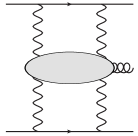
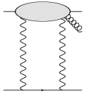
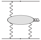
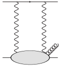
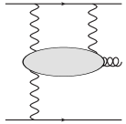
(a)

(b)

(c)

(d)

(e)

Figure 4: Different types of real NLO corrections.

Among the former class, Fig. 4.a is immediately absent due to the decoupling of the anti-symmetric color octet from the two reggeized gluon state; combined with projection of one of the $t$-channels on the color singlet, the corresponding diagrams vanish by color algebra. As we are interested in events with large rapidity gaps, also Fig. 4.c and Fig. 4.e will not contribute to the jet impact factor. These contributions become relevant if the size of the diffractive system formed by the gluon and e.g. the upper quark (in the case of Fig. 4.c) is large and a resummation of logarithms $\ln M_{X}^{2}$ becomes mandatory. Here we are not interested in such configurations and we will not pursue further this idea. These contributions provide however a cross-check on the diagrams of interest, Fig. 4.b and Fig. 4.d which describe emissions in the quasi-elastic region. In the limit of large invariant mass of the gluon and the upper/lower final state quark in Fig. 4.b/d, this contribution is required to turn into the factorized expression Fig. 4.c/e. The central production vertex is well known from the literature, both using conventional methods [23] and the effective action [24], see also [25]. For completeness its calculation will be briefly discussed in Appendix A. In principle there exist further contributions such as Fig. 5.c which contain an explicit splitting of a single reggeized gluon into two reggeized gluons. Contributions containing such splittings can be shown to vanish after integration over the longitudinal loop momentum $l^{-}$ and therefore will not be considered here.

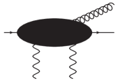
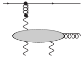
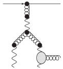
(a)

(b)

(c)

Figure 5: Different reggeized gluon diagrams contributing to the real corrections to the Mueller-Tang impact factor. (a) Quasi-elastic and (b) central production diagram. (c) Diagram with a reggeized gluon - 2 reggeized gluon splitting. The gray blob denotes an effective coupling known as the Lipatov vertex. For a derivation from the high energy effective action see [16]. Those contributions can be shown to vanish identically, if the light-cone denominator is treated with a symmetric pole prescription as proposed in [26].

In the following we determine the quasi-elastic subprocess emission of Fig. 5.a. To this end we note that the diagrams in the black blobs are understood to contain no internal reggeized gluon lines. For the determination of reggeized gluon - particle vertices, the reggeized gluon must be therefore treated as a background field, see also the discussion in [16, 17, 18] for further details. In particular, Fig. 5.b and diagrams such as Fig. 5.c are not a subset of the Feynman diagrams contributing to Fig. 5.a.

4.3 The quasi-elastic corrections

To extract the real corrections to the jet impact factor it is therefore sufficient to study the contribution corresponding to Fig. 4.b. As in Sec. 4.1, the integral over longitudinal loop momenta $l^{-}$ and $l^{+}$ factorizes and can be directly associated with the $qr^{*}r^{*}\to qg$ and $qr^{*}r^{*}\to q$ subprocesses. Generalizing the analysis carried out in Sec. 4.1 we therefore consider the process $q(p_{a})+r^{*}(l)+r^{*}(k-l)\to q(p)+g(q)$ with the following Sudakov decomposition of external momenta

$$p_{a} =p_{a}^{+}\frac{n^{-}}{2},\qquad\qquad\qquad k=k^{-}\frac{n^{+}}{2}+{\bm{k}}, l =l^{-}\frac{n^{+}}{2}+{\bm{l}},$$

$$p =(1-z)p_{a}^{+}\frac{n^{-}}{2}+\frac{{\bm{p}}^{2}}{(1-z)p_{a}^{+}}\frac{n^{+}}{2}+{\bm{p}}, q =zp_{a}^{+}\frac{n^{-}}{2}+\frac{{\bm{q}}^{2}}{zp_{a}^{+}}\frac{n^{+}}{2}+{\bm{q}}\,.$$ (35)

The necessary set of Feynman diagrams is depicted in Fig. 6.

= + + + +
+ + + + + +
+ + + + + +
+ + + + + + .

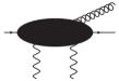
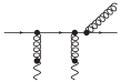
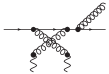
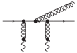
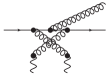
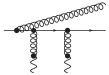
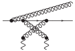
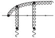
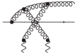
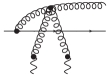
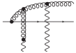
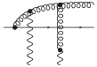
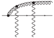
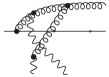
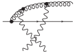
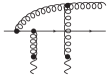
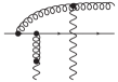
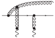
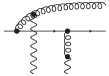
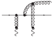
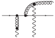
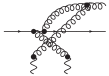
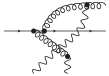
Figure 6: Real NLO diagrams: the quark + 2 reggeized gluon $\to$ quark gluon amplitude.

At amplitude level we obtain

$${i}\phi_{qqg} =\int\frac{dl^{-}}{8\pi}i\mathcal{M}^{cb_{1}b_{2}}_{q2r^{*}qg}P^{b_{1}b_{2}}={g^{3}}t^{c}\sum_{i=1}^{5}a_{i}.$$ (36)

For the evaluation of the integral over $l^{-}$, we combined diagrams with adjacent reggeized gluons (without emission of a real gluon in between), similar to the LO case Eq. (25). In this way, the convergence of all integrals is verified in a straightforward manner and the integral can be evaluated by taking residues. As a result we obtain the following five amplitudes,

$$a_{1} =-\frac{C_{f}}{2\sqrt{N_{c}^{2}-1}}\cdot\frac{z(1-z)}{{\bm{\Delta}}^{2}}\cdot{\bar{u}(p){\text{$\epsilon$$\diagup$\hskip 2.02951pt}(\text{$p$$\diagup$\hskip 2.51563pt}_{a}+\text{$k$$\diagup$\hskip 2.76042pt})\text{$n$$\diagup$\hskip 3.00117pt}^{+}}u(p_{a})},$$

$$a_{2} =\frac{C_{f}}{2\sqrt{N_{c}^{2}-1}}\cdot\frac{z}{{\bm{q}}^{2}}\cdot{\bar{u}(p){\text{$n$$\diagup$\hskip 3.00117pt}^{+}(\text{$p$$\diagup$\hskip 2.51563pt}_{a}-\text{$q$$\diagup$\hskip 2.41145pt})\text{$\epsilon$$\diagup$\hskip 2.02951pt}}u(p_{a})},$$

$$a_{3} =\frac{C_{a}}{\sqrt{N_{c}^{2}-1}}\cdot\frac{1-z}{{\bm{p}}^{2}}\cdot{\bar{u}(p)\gamma^{\rho}(zp_{a}^{+}\epsilon_{\rho}+(n^{+})^{\rho}k\cdot\epsilon)u(p_{a})},$$

$$a_{4} =\frac{C_{a}}{4\sqrt{N_{c}^{2}-1}}\cdot\frac{1}{p_{a}^{+}{\bm{\Sigma}}_{1}^{2}}\cdot\bar{u}(p){\text{$n$$\diagup$\hskip 3.00117pt}^{+}(\text{$l$$\diagup$\hskip 1.59029pt}_{i}+\text{$p$$\diagup$\hskip 2.51563pt}_{a}-\text{$q$$\diagup$\hskip 2.41145pt})(zp_{a}^{+}\epsilon_{\rho}+n^{+}_{\rho}l_{i}\cdot\epsilon)\gamma^{\rho}}u(p_{a}),$$

$$a_{5} =\frac{C_{a}}{4\sqrt{N_{c}^{2}-1}}\cdot\frac{1}{p_{a}^{+}{\bm{\Upsilon}}_{1}^{2}}\cdot\bar{u}(p){\text{$n$$\diagup$\hskip 3.00117pt}^{+}(\text{$k$$\diagup$\hskip 2.76042pt}-\text{$l$$\diagup$\hskip 1.59029pt}_{i}+\text{$p$$\diagup$\hskip 2.51563pt}_{a}-\text{$q$$\diagup$\hskip 2.41145pt})(zp_{a}^{+}\epsilon_{\rho}+n^{+}_{\rho}(k\cdot\epsilon-l_{i}\cdot\epsilon))\gamma^{\rho}}u(p_{a}),$$ (37)

where $l_{i}$, $i=1,2$ is the loop momenta of the reggeized gluon loop with $i=1$ assigned to the amplitude and $i=2$ to its complex conjugate. We also defined the transverse momenta

$${\bm{\Delta}} ={\bm{q}}-z{\bm{k}}, {\bm{\Sigma}}_{i} ={\bm{q}}-{\bm{l}}_{i}, {\bm{\Upsilon}}_{i} ={\bm{q}}-{\bm{k}}+{\bm{l}}_{i} i =1,2.$$ (38)

With the 2-particle phase space

$$d\Phi^{(2)} =\frac{1}{(4\pi)^{1+\epsilon}}\int\frac{dz}{2p_{a}^{+}z(1-z)}\int\frac{d^{2+2\epsilon}{\bm{q}}}{\pi^{1+\epsilon}}\delta\left(k^{-}-\frac{{\bm{\Delta}}^{2}+z(1-z){\bm{k}}^{2}}{(1-z)zp_{a}^{+}}\right)$$ (39)

and the invariant mass of the final state quark-gluon system

$$\hat{M}_{X}^{2} =(p_{a}+k)^{2}=\frac{{\bm{\Delta}}^{2}}{z(1-z)}<xM_{X,\text{max}}^{2}-(1-x){\bm{k}}^{2}\equiv\hat{M}_{X,\text{max}}^{2},$$ (40)

we obtain

$$h^{(1)}_{r,qg}d[{\bm{q}}]dz=\frac{1}{2}\sum_{\text{spin}}\frac{1}{N_{c}}\sum_{\text{color}}\int dk^{-}\frac{\Theta\left(M_{X,\text{max}}^{2}-M_{X}^{2}\right)}{2^{-\epsilon}p_{a}^{+}(2\pi)(4\pi)^{2+2\epsilon}}\left(\sum_{i}^{5}a_{i}\right)\left(\sum_{i}^{5}a_{i}^{\dagger}\right)d\Phi^{(2)}$$

$$=h^{(0)}\frac{\alpha_{s,\epsilon}}{2\pi}\frac{P_{gq}(z,\epsilon)}{\Gamma(1-\epsilon)\mu^{2\epsilon}}\left[C_{f}\left(\frac{{\bm{\Delta}}}{{\bm{\Delta}}^{2}}-\frac{{\bm{q}}}{{\bm{q}}^{2}}\right)-{C_{a}}\left(\frac{{\bm{p}}}{{\bm{p}}^{2}}+\frac{1}{2}\frac{{\bm{\Sigma}}_{1}}{{\bm{\Sigma}}_{1}^{2}}+\frac{1}{2}\frac{{\bm{\Upsilon}}_{1}}{{\bm{\Upsilon}}^{2}_{1}}\right)\right]\cdot\bigg{[}C_{f}\left(\frac{{\bm{\Delta}}}{{\bm{\Delta}}^{2}}-\frac{{\bm{q}}}{{\bm{q}}^{2}}\right)$$

$$-{C_{a}}{}\left(\frac{{\bm{p}}}{{\bm{p}}^{2}}+\frac{1}{2}\frac{{\bm{\Sigma}}_{2}}{{\bm{\Sigma}}_{2}^{2}}+\frac{1}{2}\frac{{\bm{\Upsilon}}_{2}}{{\bm{\Upsilon}}^{2}_{2}}\right)\bigg{]}\Theta\left(x{M_{X,\text{max}}^{2}-(1-x){\bm{k}}^{2}}-\frac{{\bm{\Delta}}^{2}}{z(1-z)}\right)d[{\bm{q}}]dz,$$ (41)

where

$$P_{gq}(z,\epsilon) =C_{f}\frac{1+(1-z)^{2}+\epsilon z^{2}}{z}$$ (42)

is the real part of the $q\to g$ splitting function and we used the shorthand expression $d[{\bm{k}}]\equiv d^{2+2\epsilon}{\bm{k}}/\pi^{1+\epsilon}$. Organizing the terms according to their color coefficient we arrive at

$$h^{(1)}_{r,qg}= h^{(0)}\frac{\alpha_{s,\epsilon}}{2\pi}\frac{P_{gq}(z,\epsilon)}{\Gamma(1-\epsilon)\mu^{2\epsilon}}\Theta\left(\hat{M}_{X,{\rm max}}^{2}-\frac{{\bm{\Delta}}^{2}}{z(1-z)}\right)$$

$$\qquad\qquad\bigg{\{}C_{f}^{2}\frac{z^{2}{\bm{k}}^{2}}{{\bm{\Delta}}^{2}{\bm{q}}^{2}}+{C_{a}}{C_{f}}\bigg{(}J_{1}({\bm{q}},{\bm{k}},{\bm{l}}_{1},z)+J_{1}({\bm{q}},{\bm{k}},{\bm{l}}_{2},z)\bigg{)}+C_{a}^{2}J_{2}({\bm{q}},{\bm{k}},{\bm{l}}_{1},{\bm{l}}_{2})\bigg{\}},$$ (43)

where

$$J_{1}({\bm{q}},{\bm{k}},{\bm{l}}_{i},z) =\frac{1}{4}\bigg{[}2\frac{{\bm{k}}^{2}}{{\bm{p}}^{2}}\bigg{(}\frac{(1-z)^{2}}{{\bm{\Delta}}^{2}}-\frac{1}{{\bm{q}}^{2}}\bigg{)}-\frac{1}{{\bm{\Sigma}}_{i}^{2}}\bigg{(}\frac{({\bm{l}}_{i}-z{\bm{k}})^{2}}{{\bm{\Delta}}^{2}}-\frac{{\bm{l}}_{i}^{2}}{{\bm{q}}^{2}}\bigg{)}$$

$$\qquad\qquad\qquad\qquad-\frac{1}{{\bm{\Upsilon}}_{i}^{2}}\bigg{(}\frac{({\bm{l}}_{i}-(1-z){\bm{k}})^{2}}{{\bm{\Delta}}^{2}}-\frac{({\bm{l}}_{i}-{\bm{k}})^{2}}{{\bm{q}}^{2}}\bigg{)}\bigg{]};$$

$$J_{2}({\bm{q}},{\bm{k}},{\bm{l}}_{1},{\bm{l}}_{2}) =\frac{1}{4}\bigg{[}\frac{{\bm{l}}_{1}^{2}}{{\bm{p}}^{2}{\bm{\Upsilon}}^{2}_{1}}+\frac{({\bm{k}}-{\bm{l}}_{1})^{2}}{{\bm{p}}^{2}{\bm{\Sigma}}^{2}_{1}}+\frac{{\bm{l}}_{2}^{2}}{{\bm{p}}^{2}{\bm{\Upsilon}}^{2}_{2}}+\frac{({\bm{k}}-{\bm{l}}_{2})^{2}}{{\bm{p}}^{2}{\bm{\Sigma}}^{2}_{2}}$$

$$-\frac{1}{2}\bigg{(}\frac{({\bm{l}}_{1}-{\bm{l}}_{2})^{2}}{{\bm{\Sigma}}_{1}^{2}{\bm{\Sigma}}_{2}^{2}}+\frac{({\bm{k}}-{\bm{l}}_{1}-{\bm{l}}_{2})^{2}}{{\bm{\Upsilon}}_{1}^{2}{\bm{\Sigma}}_{2}^{2}}+\frac{({\bm{k}}-{\bm{l}}_{1}-{\bm{l}}_{2})^{2}}{{\bm{\Sigma}}_{1}^{2}{\bm{\Upsilon}}_{2}^{2}}+\frac{({\bm{l}}_{1}-{\bm{l}}_{2})^{2}}{{\bm{\Upsilon}}_{1}^{2}{\bm{\Upsilon}}_{2}^{2}}\bigg{)}\bigg{]}.$$ (44)

With

$$\hat{M}_{X}^{2} =\left(\frac{{\bm{q}}^{2}}{z}+\frac{{\bm{p}}^{2}}{1-z}-{\bm{k}}^{2}\right)\;,$$ (45)

large partonic diffractive mass corresponds to the limits $z\to 0$ and $z\to 1$ at fixed transverse gluon and quark momentum respectively. For $z\to 1$ we find that Eq. (B) is finite and no high energy singularity is present. This is to be expected as this case corresponds to highly negative rapidities of the real quark, which are power suppressed in the high energy limit. For $z\to 0$ we find, on the other hand, that the term proportional to the color factor $C_{a}^{2}$ contains a high energy singularity $1/z$. Meanwhile, the terms proportional to $C_{f}^{2}$ and $C_{f}C_{a}$ vanish in the limit $z\to 0$ and hence cancel the singularity present in $P_{gq}(z,\epsilon)$. It is then straightforward to check that the singular term agrees precisely with the high energy factorized cross-section of Eq. (98) derived in the Appendix A, thus validating the correctness of our result in this limit.

5 The jet vertex for quark induced jets with rapidity gap

To obtain from the partonic real NLO corrections in Eq. (4.3) for the jet vertex, we need to combine this result with the corresponding virtual corrections, add a jet definition and absorb initial state singularities into parton distribution functions. We follow here closely the corresponding treatment in the case of Mueller-Navelet jets discussed in [28, 29].

5.1 Virtual corrections and renormalization

The virtual corrections have been calculated in [12]. Unlike the present calculation, the authors of [12] make no use of Lipatov’s effective action, but calculate the corresponding corrections directly from QCD Feynman diagrams with the help of dispersion relations, employing analyticity and unitarity of QCD scattering amplitudes. The virtual corrections are then given as the sum of quark-intermediate state impact factor and quark-gluon-intermediate quark impact factor, where the terminology appears natural from the calculational method of [12]. The result for the quark-gluon-intermediate state is given in Eq. (6.19) of [12]. Projected on the color singlet it reads at cross-section level

$$h^{(1)}_{v,a}({{\bm{k}},{\bm{l}}_{1}},{\bm{l}}_{2}) =C_{f}^{2}h^{(0)}{\frac{(4\pi)^{1+\epsilon}\alpha_{s,\epsilon}}{\mu^{2\epsilon}\Gamma(1-\epsilon)}}\bigg{\{}-C_{f}I_{B}^{(+)}({\bm{l}}_{1},{\bm{k}})-\frac{C_{a}}{2}\big{[}\tilde{I}_{A}^{(+)}({\bm{l}}_{1},{\bm{k}})$$

$$\qquad\qquad\qquad\qquad\qquad-I_{B}^{(+)}({\bm{l}}_{1},{\bm{k}})+\tilde{I}_{C}^{(+)}({\bm{l}}_{1},{\bm{k}})\big{]}+({\bm{l}}_{1})\leftrightarrow({\bm{l}}_{2})\bigg{\}}.$$ (46)

The functions $\tilde{I}_{A}^{(+)}$, ${I}_{B}^{(+)}$ and $\tilde{I}_{C}^{(+)}$ are given in Eqs. (6.11), (6.18) and (6.15) of [12]. The quark intermediate state reads at cross-section level, after projection on the color singlet

$$h^{(1)}_{v,b}({\bm{k}},{\bm{l}}_{1},{\bm{l}}_{2}) =C_{f}^{2}h^{(0)}\frac{\alpha_{s,\epsilon}\Gamma^{2}(1+\epsilon)}{4\pi\Gamma(1+2\epsilon)(-\epsilon)}\bigg{\{}\left[\left(\frac{{\bm{l}}_{1}^{2}}{\mu^{2}}\right)^{\epsilon}+\left(\frac{({\bm{k}}-{\bm{l}}_{1})^{2}}{\mu^{2}}\right)^{\epsilon}\right]\bigg{[}\frac{-n_{f}(1+\epsilon)}{(1+2\epsilon)(3+2\epsilon)}$$

$$+(2C_{f}-C_{a})\left(\frac{1}{\epsilon(1+2\epsilon)}+\frac{1}{2}\right)+C_{a}\bigg{(}\psi(1-\epsilon)-2\psi(\epsilon)+\psi(1)$$

$$+\frac{1}{4(1+2\epsilon)(3+2\epsilon)}-\frac{1}{\epsilon(1+2\epsilon)}-\frac{7}{4(1+2\epsilon)}\bigg{)}\bigg{]}$$

$$\qquad+C_{a}\bigg{[}\ln\frac{s_{0}}{{\bm{l}}_{1}^{2}}\left(\frac{{\bm{l}}_{1}^{2}}{\mu^{2}}\right)^{\epsilon}+\ln\frac{s_{0}}{({\bm{k}}-{\bm{l}}_{1})^{2}}\left(\frac{({\bm{k}}-{\bm{l}}_{1})^{2}}{\mu^{2}}\right)^{\epsilon}\bigg{]}+({\bm{l}}_{1})\leftrightarrow({\bm{l}}_{2})\bigg{\}}.$$ (47)

$s_{0}$ denotes here the reggeization scale, which sets the scale of the energy logarithms, resummed by the non-forward BFKL Green’s function; $\mu^{2}$ is the scale of dimensional regularization and $\beta_{0}=\frac{11}{3}N_{c}-\frac{2}{3}n_{f}$. Expanding in $\epsilon$ we find for the virtual corrections

$$h^{(1)}_{v} =h_{v,a}^{(1)}({\bm{k}},{\bm{l}}_{1},{\bm{l}}_{2})+h_{v,b}^{(1)}({\bm{k}},{\bm{l}}_{1},{\bm{l}}_{2}),$$ (48)

the following terms

$$h^{(1)}_{v}={h^{(0)}}C_{f}^{2}\frac{\alpha_{s,\epsilon}}{4\pi}\bigg{\{}-2\frac{\beta_{0}}{\epsilon}{-\frac{\beta_{0}}{2}\left[\left\{\ln\left(\frac{\bm{l}_{1}^{2}}{\mu^{2}}\right)+\ln\left(\frac{(\bm{l}_{1}-\bm{k})^{2}}{\mu^{2}}\right)+\{1\leftrightarrow 2\}\right\}-\frac{20}{3}\right]}$$

$$+2{C_{f}}\left[-\frac{2}{\epsilon^{2}}+\frac{1}{\epsilon}\left(3-2\ln\left(\frac{{\bm{k}}^{2}}{\mu^{2}}\right)\right){-\ln^{2}\left(\frac{\bm{k}^{2}}{\mu^{2}}\right)+3\ln\left(\frac{\bm{k}^{2}}{\mu^{2}}\right)+\frac{\pi^{2}}{3}-8}\right]$$

$${+C_{a}\bigg{[}\bigg{\{}\frac{3}{2\bm{k}^{2}}\left\{\bm{l}_{1}^{2}\ln\left(\frac{(\bm{l}_{1}-\bm{k})^{2}}{\bm{l}_{1}^{2}}\right)+(\bm{l}_{1}-\bm{k})^{2}\ln\left(\frac{\bm{l}_{1}^{2}}{(\bm{l}_{1}-\bm{k})^{2}}\right)-4|\bm{l}_{1}||\bm{l}_{1}-\bm{k}|\phi_{1}\sin\phi_{1}\right\}}$$

$$\quad\quad{-\frac{3}{2}\left[\ln\left(\frac{\bm{l}_{1}^{2}}{\bm{k}^{2}}\right)+\ln\left(\frac{(\bm{l}_{1}-\bm{k})^{2}}{\bm{k}^{2}}\right)\right]-\ln\left(\frac{\bm{l}_{1}^{2}}{\bm{k}^{2}}\right)\ln\left(\frac{(\bm{l}_{1}-\bm{k})^{2}}{s_{0}}\right)}$$

$$\quad\quad{-\ln\left(\frac{(\bm{l}_{1}-\bm{k})^{2}}{\bm{k}^{2}}\right)\ln\left(\frac{\bm{l}_{1}^{2}}{s_{0}}\right)-2\phi_{1}^{2}+\{1\leftrightarrow 2\}\bigg{\}}+2\pi^{2}+\frac{14}{3}\bigg{]}}+{\cal{O}(\epsilon)\bigg{\}}}.$$ (49)

Here

$$\phi_{i} =\arccos\frac{{\bm{k}}^{2}-{\bm{l}}_{i}^{2}-({\bm{k}-{\bm{l}}_{i})^{2}}}{{2}|{\bm{l}}_{i}||{\bm{l}}_{i}-{\bm{k}}|}, i =1,2,$$ (50)

denotes the angle between the reggeized gluon momenta with $|\phi_{i}|\leq\pi$, $i=1,2$. The first divergent term is of ultraviolet origin and comes multiplied by the first term of the QCD $\beta$ function. Employing renormalization of the QCD Lagrangian within the $\overline{\text{MS}}$ scheme

$$\alpha_{s}(\mu) =\alpha_{s,\epsilon}\left[1-\frac{\alpha_{s,\epsilon}\beta_{0}}{4\pi\epsilon}\right],$$ (51)

this term will be canceled. The remaining divergences are of soft or collinear origin. They will be partly canceled by corresponding singularities in the real corrections, with the remainder to be absorbed by collinear factorization.

5.2 The jet vertex at partonic and hadronic level at leading order

To extract the jet vertex at partonic level, we need to combine the results obtained so far with a jet function, following Eq. (10). Due to high energy factorization of the cross-section, it is possible to carry out this analysis separately for each impact factor. To be more precise, we write the differential partonic jet cross-section in its most general form as

$$\frac{d\hat{\sigma}}{dJ_{1}\,dJ_{2}\,\,d^{2}{\bm{k}}} =\int\frac{d^{2}{\bm{l}}_{1}}{\pi}\int\frac{d^{2}{\bm{l}}^{\prime}_{1}}{\pi}\int\frac{d^{2}{\bm{l}}_{2}}{\pi}\int\frac{d^{2}{\bm{l}}^{\prime}_{2}}{\pi}\frac{d\hat{V}({\bm{l}}_{1},{\bm{l}}_{2},{\bm{k}},{\bm{p}}_{J,1},{y}_{1},s_{0})}{dJ_{1}}$$

$$\qquad\qquad\qquad G\left({\bm{l}}_{1},{\bm{l}}_{1}^{\prime},{\bm{k}},\frac{\hat{s}}{s_{0}}\right)G\left({\bm{l}}_{2},{\bm{l}}_{2}^{\prime},{\bm{k}},\frac{\hat{s}}{s_{0}}\right)\frac{d\hat{V}({\bm{l}}^{\prime}_{1},{\bm{l}}^{\prime}_{2},{\bm{k}},{\bm{p}}_{J,2},{y}_{2},s_{0})}{dJ_{2}},$$ (52)

where $G$ denotes the non-forward BFKL Green’s function which is either taken in the asymptotic limit $\ln\hat{s}/s_{0}\to\infty$ or implies a suitable infrared regulator. If the final state is given by a single quark, the jet definition is trivial and given by Eq. (11). We find in that case

$$\frac{d\hat{V}_{q}}{dJ} =v^{(0)}_{q}S^{(2)}_{J}({\bm{\bm{k}}},x), v_{q}^{(0)} =\frac{\alpha_{s}^{2}C_{f}^{2}}{N_{c}^{2}-1}.$$ with (53)

An identical expression holds for the virtual corrections in Eq. (5.1), but with $h^{(0)}_{q}$ replaced by $h^{(1)}_{v}$. In the following we assume that the reggeization scale $s_{0}$ is chosen such that the BFKL Green’s functions do not explicitly depend on the proton momentum fractions $x_{1}$ and $x_{2}$ of the initial quarks. Examples of such choices for $s_{0}$ are $\log s/s_{0}=\Delta\eta$ where $\eta$ denotes multiples of either the separation of the jets in rapidity $\Delta y$ or the size of the gap $\Delta y_{\text{gap}}$. For such scenarios we can define

$$\frac{dV_{q}^{(0)}}{dJ} =\int_{x_{0}}^{1}dx\,\,f_{q/H}(x,\mu_{F}^{2})\,h_{q}^{(0)}\,S^{(2)}_{J}({\bm{p}},x)$$

$$=v_{q}^{(0)}\cdot x_{J}f_{q/H}(x_{J},\mu_{F}^{2})\,\delta^{(2)}({\bm{p}}-{\bm{k}}_{J}),\qquad\qquad\qquad x_{0}<x_{J}=\frac{|{\bm{k}}_{J}|{e^{y_{J}}}}{\sqrt{s}}<1,$$ (54)

and the corresponding hadronic cross-section is given by Eq. (5.2) with all ‘hats’ removed.

5.3 Next-to-leading order vertex: jet function

As soon as the final state is no longer given by a single quark, the jet function is no longer trivial and some dependence on the chosen jet algorithm enters. Since the additional final state gluon may be soft or collinear to either initial or final state quark, the jet function needs to fulfill the following set of requirements [30], to guarantee infrared finiteness of the cross-section. For a general partonic process with momenta $p_{a}+p_{b}\to p_{1}+\ldots p_{n}$ the jet function for $n$ final state particles $S_{J}^{n}(p_{1}...,p_{n},;p_{a},p_{b})$ reduces to the jet function of $n-1$ final state particles in the following way. If the particle $j$ is soft,

$$\lim_{p_{j}\to 0}S_{J}^{n}(p_{1}\ldots,p_{j},\ldots,p_{n};p_{a},p_{b})=S_{J}^{n-1}(p_{1},\ldots,\hat{p}_{j},\ldots,p_{n};p_{a},p_{b}),$$ (55)

where $\hat{p}_{j}$ indicates omission of the $j$-th particle. If two final state partons with index $i$ and $j$ are collinear, $p_{i}=a\cdot p$ and $p_{j}=b\cdot p$,

$$S_{J}^{n}(\ldots,a\cdot p,\ldots,b\cdot p,\ldots,;p_{a},p_{b})=S_{J}^{n-1}(p_{1}\ldots,(a+b)\cdot p,\ldots p_{n};p_{a},p_{b})\;,$$ (56)

and if a final state parton with index $i$ is collinear to an initial state parton, $p_{i}=a\cdot p_{a}$

$$S_{J}^{n}(p_{1},\ldots,a\cdot p_{a},\ldots,p_{n};p_{a},p_{b})=S_{J}^{n-1}(p_{1},\ldots,\hat{p}_{i},\ldots p_{n};(1-a)\cdot p_{a},p_{b}).$$ (57)

In the present case, with the phase space of the final quark-gluon system parametrized both by longitudinal momentum fraction, carried forward from the initial quark with momentum fraction $x$ by gluon ($z$) and quark (${\bar{z}}=1-z$), and gluon (${\bm{p}}$) and quark (${\bm{q}}$) transverse momentum, these conditions can be expressed as follows

$$S_{J}^{(3)}({\bm{p}},{\bm{q}},zx,x) \to S_{J}^{(2)}({\bm{p}},x) {\bm{q}}\to 0,z\to 0$$

$$S_{J}^{(3)}({\bm{p}},{\bm{q}},zx,x) \to S_{J}^{(2)}({\bm{k}},x) \frac{{\bm{q}}}{z}\to\frac{{\bm{p}}}{1-z}$$

$$S_{J}^{(3)}({\bm{p}},{\bm{q}},zx,x) \to S_{J}^{(2)}({\bm{k}},(1-z)x) {\bm{q}}\to 0$$

$$S_{J}^{(3)}({\bm{p}},{\bm{q}},zx,x) \to S_{J}^{(2)}({\bm{k}},zx) {\bm{p}}\to 0,$$

together with symmetry of $S^{(3)}$ under the simultaneous swapping of ${\bm{p}}\leftrightarrow{\bm{q}}$ and $z\leftrightarrow 1-z$. While finiteness of the jet impact factor is generally expected due to these particular constraints imposed onto the jet definition, we note that the verification of the latter is non-trivial in the present case due to high energy factorization of the partonic cross-section into jet impact factors and two reggeized gluon exchange.

5.4 Next-to-leading order jet vertex: different contributions

The virtual part of the one-loop corrections to the jet vertex follows exactly the tree-level result. After renormalization within the $\overline{\text{MS}}$ scheme, following Eq. (51), we split the virtual corrections into a finite term and a term which gathers the entire set of so-far uncanceled soft and collinear singularities,

$$\frac{d\hat{V}_{v}^{(1)}}{dJ} =\frac{d\hat{V}_{v,\text{sc}}^{(1)}}{dJ}+\frac{d\hat{V}_{v,\text{finite}}^{(1)}}{dJ},$$ (59)

with

$$\frac{d\hat{V}_{v,\text{sc}}^{(1)}}{dJ} =S_{J}^{(2)}({\bm{k}},x)\cdot{h^{(0)}}C_{f}^{3}\frac{\alpha_{s}}{2\pi}\bigg{(}-\frac{2}{\epsilon^{2}}+\frac{3}{\epsilon}-\frac{2}{\epsilon}\ln\frac{{\bm{k}}^{2}}{\mu^{2}}\bigg{)}$$ (60)

and

$$\frac{d\hat{V}_{v,\text{finite}}^{(1)}}{dJ} =S_{J}^{(2)}({\bm{k}},x)\cdot v^{(0)}_{q}\cdot\frac{\alpha_{s}}{4\pi}\bigg{\{}{-\frac{\beta_{0}}{2}\left[\left\{\ln\left(\frac{\bm{l}_{1}^{2}}{\mu^{2}}\right)+\ln\left(\frac{(\bm{l}_{1}-\bm{k})^{2}}{\mu^{2}}\right)+\{1\leftrightarrow 2\}\right\}-\frac{20}{3}\right]}$$

$$+2{C_{f}}\left[{-\ln^{2}\left(\frac{\bm{k}^{2}}{\mu^{2}}\right)+3\ln\left(\frac{\bm{k}^{2}}{\mu^{2}}\right)+\frac{\pi^{2}}{3}-8}\right]$$

$$+{C_{a}\bigg{[}\bigg{\{}\frac{3}{2\bm{k}^{2}}\left\{\bm{l}_{1}^{2}\ln\left(\frac{(\bm{l}_{1}-\bm{k})^{2}}{\bm{l}_{1}^{2}}\right)+(\bm{l}_{1}-\bm{k})^{2}\ln\left(\frac{\bm{l}_{1}^{2}}{(\bm{l}_{1}-\bm{k})^{2}}\right)-4|\bm{l}_{1}||\bm{l}_{1}-\bm{k}|\phi_{1}\sin\phi_{1}\right\}}$$

$$\quad\quad{-\frac{3}{2}\left[\ln\left(\frac{\bm{l}_{1}^{2}}{\bm{k}^{2}}\right)+\ln\left(\frac{(\bm{l}_{1}-\bm{k})^{2}}{\bm{k}^{2}}\right)\right]-\ln\left(\frac{\bm{l}_{1}^{2}}{\bm{k}^{2}}\right)\ln\left(\frac{(\bm{l}_{1}-\bm{k})^{2}}{s_{0}}\right)}$$

$$\quad\quad{-\ln\left(\frac{(\bm{l}_{1}-\bm{k})^{2}}{\bm{k}^{2}}\right)\ln\left(\frac{\bm{l}_{1}^{2}}{s_{0}}\right)-2\phi_{1}^{2}+\{1\leftrightarrow 2\}\bigg{\}}+2\pi^{2}+\frac{14}{3}\bigg{]}\bigg{\}}}.$$ (61)

To obtain from the NLO partonic cross-section a finite NLO collinear coefficient, we further need to absorb initial state collinear singularities into parton distribution functions. This can be achieved by adding suitable counterterms to the partonic NLO cross-section. At the level of the jet vertex in Eq. (5.2) the counterterms read (in the $\overline{\text{MS}}$-scheme)

$$\frac{dV^{(1)}_{ct}}{dJ} =\int_{x_{0}}^{1}dx\,\,f_{q}\left(x,\mu_{F}^{2}\right)\frac{d\hat{V}^{(1)}_{ct}}{dJ},\qquad\frac{d\hat{V}^{(1)}_{ct}}{dJ}=\frac{d\hat{V}^{(1)}_{ct,q}}{dJ}+\frac{d\hat{V}^{(1)}_{ct,g}}{dJ};$$

$$\frac{d\hat{V}^{(1)}_{ct,q}}{dJ} =-\frac{\alpha_{s,\epsilon}}{2\pi}\left(\frac{1}{\epsilon}+\ln\frac{\mu_{F}^{2}}{\mu^{2}}\right)\int_{z_{0}}^{1}{dz}\,\,S_{J}^{(2)}({\bm{k}},zx)\cdot h_{q}^{(0)}P_{qq}^{(0)}(z),$$

$$\frac{d\hat{V}^{(1)}_{ct,g}}{dJ} =-\frac{\alpha_{s,\epsilon}}{2\pi}\left(\frac{1}{\epsilon}+\ln\frac{\mu_{F}^{2}}{\mu^{2}}\right)\int_{z_{0}}^{1}{dz}\,\,S_{J}^{(2)}({\bm{k}},zx)\cdot h^{(0)}_{g}{P_{gq}^{(0)}}(z)\,,$$ (62)

with the LO splitting functions

$$P_{qq}^{(0)}(z) =C_{f}\left(\frac{1+z^{2}}{1-z}\right)_{+}, P_{gq}^{(0)}(z) =C_{f}\frac{1+(1-z)^{2}}{z}\,,$$ (63)

and the plus distribution

$$\int_{\alpha}^{1}dx\,\,f(x)[g(x)]_{+} \equiv\int_{\alpha}^{1}dx\,\,\big{(}f(x)-f(1)\big{)}g(x)-f(1)\int_{0}^{\alpha}dx\,\,g(x)\,.$$ (64)

For the lower bound $z_{0}$ we notice that we can use the combination of splitting function and LO partonic cross-section $\hat{M}_{X}^{2}=\frac{{\bm{k}}^{2}(1-z)}{z}$ and write

$$z_{0} =\frac{{\bm{k}}^{2}/x}{M_{X,\text{max}}^{2}+{\bm{k}}^{2}}\,\,.$$ (65)

The real corrections are finally given by

$$\frac{dV^{(1)}_{r}}{dJ} =\int_{x_{0}}^{1}dx\,\,f_{q/H}(x,\mu_{F}^{2})\,\frac{d\hat{V}^{(1)}_{r}}{dJ},$$

$$\frac{d\hat{V}^{(1)}_{r}}{dJ} =\int_{0}^{1}dz\int\frac{d^{2+2\epsilon}{\bm{q}}}{\pi^{1+\epsilon}}\,\,h^{(1)}_{r,qg}S_{J}^{(3)}({\bm{p}},{\bm{q}},zx,x).$$ (66)

To extract the soft and collinear singularities from the latter, we first decompose $h^{(1)}_{r}$ according to its color structure, following Eqs. (4.3), (4.3). We start with the terms proportional to $C_{f}^{2}$. Substituting $z\to 1-z$ and rescaling the gluon transverse momentum ${\bm{q}}\to(1-z){\bm{q}}$, where $z$ indicates now the momentum fraction carried by the final state quark, we have

$$\left(\frac{d\hat{V}^{(1)}_{r}}{dJ}\right)_{C_{f}^{2}} =\int_{0}^{1}dz\int\frac{d^{2+2\epsilon}{\bm{q}}}{\pi^{1+\epsilon}}h^{(0)}\frac{\alpha_{s,\epsilon}}{2\pi}\frac{C_{f}^{3}}{\Gamma(1-\epsilon)\mu^{2\epsilon}}\frac{1+z^{2}+\epsilon(1-z)^{2}}{(1-z)^{1-2\epsilon}}\frac{{\bm{k}}^{2}}{{\bm{q}}^{2}({\bm{q}}-{\bm{k}})^{2}}$$

$$\times S_{J}^{(3)}({\bm{k}} -(1-z){\bm{q}},(1-z){\bm{q}},(1-z)x,x)\Theta\left(\frac{\hat{M}_{X,{\rm max}}^{2}}{(1-z)}-\frac{({\bm{q}}-{\bm{k}})^{2}}{z}\right).$$ (67)

The next step is to decompose the denominator in the first line

$$C_{f}\frac{1+z^{2}+\epsilon(1-z)^{2}}{(1-z)^{1-2\epsilon}} =C_{f}\left(\frac{1}{\epsilon}-\frac{3}{2}\right)\delta(1-z)+P_{qq}(z)+$$

$$\qquad\epsilon\cdot C_{f}\cdot\left[(1-z)^{1+2\epsilon}+2(1+z^{2})\left(\frac{\ln(1-z)}{1-z}\right)_{+}\right]+\mathcal{O}(\epsilon^{2}),$$ (68)

using the identity

$$(1-z)^{2\epsilon-1} =\frac{1}{2\epsilon}\delta(1-z)+\frac{1}{(1-z)_{+}}+2\epsilon\left(\frac{\ln(1-z)}{1-z}\right)_{+}+\mathcal{O}(\epsilon^{2}),$$ (69)

and split Eq. (5.4) into the three corresponding terms

$$\left(\frac{d\hat{V}^{(1)}_{r}}{dJ}\right)_{C_{f}^{2}} =\left(\frac{d\hat{V}^{(1)}_{r}}{dJ}\right)_{C_{f}^{2},a}+\left(\frac{d\hat{V}^{(1)}_{r}}{dJ}\right)_{C_{f}^{2},b}+\left(\frac{d\hat{V}^{(1)}_{r}}{dJ}\right)_{C_{f}^{2},c}+\mathcal{O}(\epsilon)\,.$$ (70)

For the first term the jet function turns out to be trivial and we obtain (up to ${\cal O}(\epsilon)$)

$$\left(\frac{d\hat{V}^{(1)}_{r}}{dJ}\right)_{C_{f}^{2},a} =h^{(0)}\frac{\alpha_{s,\epsilon}C^{3}_{f}}{2\pi}\left(\frac{2}{\epsilon^{2}}-\frac{3}{\epsilon}+\frac{2}{\epsilon}\ln\frac{{\bm{k}}^{2}}{\mu^{2}}-\frac{\pi^{2}}{3}-3\ln\frac{{\bm{k}}^{2}}{\mu^{2}}+\ln^{2}\frac{{\bm{k}}^{2}}{\mu^{2}}\right)S_{J}^{(2)}({\bm{k}},x).$$ (71)

The emerging poles in $1/\epsilon$ of this term cancel precisely against the corresponding singularities in the virtual corrections in Eq. (60). For the second term we find

$$\left(\frac{d\hat{V}^{(1)}_{r}}{dJ}\right)_{C_{f}^{2},b}=\int_{0}^{1}dz\int\frac{d^{2+2\epsilon}{\bm{q}}}{\pi^{1+\epsilon}}h^{(0)}\frac{\alpha_{s,\epsilon}}{2\pi}\frac{C_{f}^{2}}{\Gamma(1-\epsilon)\mu^{2\epsilon}}P_{qq}(z)\cdot\frac{{\bm{k}}^{2}}{{\bm{q}}^{2}({\bm{q}}-{\bm{k}})^{2}}$$

$$\quad\cdot\Theta\left(\frac{\hat{M}_{X,{\rm max}}^{2}}{(1-z)}-\frac{({\bm{q}}-{\bm{k}})^{2}}{z}\right)\cdot\,S_{J}^{(3)}({\bm{k}}-(1-z){\bm{q}},(1-z){\bm{q}},(1-z)x,x).$$ (72)

To isolate singular configurations with a final state gluon (${\bm{q}}^{2}=0$) and a final state quark ($({\bm{q}}-{\bm{k}})^{2}=0$) collinear to the initial quark, we introduce a phase space slicing parameter $\lambda$. Since

$$\lim_{{\bm{q}}^{2}\to 0}S_{J}^{(3)}({\bm{k}}-(1-z){\bm{q}},(1-z){\bm{q}},(1-z)x,x) =S_{J}^{(2)}({\bm{k}},zx),$$ (73)

we find for ${\bm{q}}^{2}<\lambda^{2}$ with ${\bm{k}}^{2}\gg\lambda^{2}\to 0$

$$\left(\frac{d\hat{V}^{(1)}_{r}}{dJ}\right)_{C_{f}^{2},b,\lambda} =\int\frac{d^{2+2\epsilon}{\bm{q}}}{\pi^{1+\epsilon}}\frac{\Theta({\lambda^{2}}-{\bm{q}}^{2})}{{\bm{q}}^{2}}h^{(0)}C_{f}^{2}\frac{\alpha_{s,\epsilon}}{2\pi}$$

$$\qquad\times\int_{0}^{1}dz\frac{P_{qq}(z)S_{J}^{(2)}({\bm{k}},zx)}{\Gamma(1-\epsilon)\mu^{2\epsilon}}\Theta\left(\frac{\hat{M}_{X,{\rm max}}^{2}}{1-z}-\frac{{\bm{k}}^{2}}{z}\right)$$

$$=\frac{\alpha_{s,\epsilon}}{2\pi}\left(\frac{1}{\epsilon}+\ln\frac{\lambda^{2}}{\mu^{2}}\right)\int_{z_{0}}^{1}dz\,\,h_{q}^{(0)}S_{J}^{(2)}({\bm{k}},zx)P_{qq}(z)+\mathcal{O}(\epsilon).$$ (74)

Adding the first collinear counterterm,

$$\left(\frac{d\hat{V}^{(1)}_{r}}{dJ}\right)_{C_{f}^{2},b,\lambda}+\left(\frac{d\hat{V}^{(1)}_{r}}{dJ}\right)_{ct,q} =v_{q}^{(0)}\cdot\frac{\alpha_{s}}{2\pi}\ln\frac{\lambda^{2}}{\mu^{2}_{F}}\int_{z_{0}}^{1}dz\,\,S_{J}^{(2)}({\bm{k}},zx)P_{qq}(z)+\mathcal{O}(\epsilon),$$ (75)

this contribution turns out to be finite. Since

$$\lim_{({\bm{q}}-{\bm{k}})^{2}\to 0}S_{J}^{(3)}({\bm{k}}-(1-z){\bm{q}},(1-z){\bm{q}},(1-z)x,x) =S_{J}^{(2)}({\bm{k}},x),$$ (76)

and

$$\int_{0}^{1}dz\,\,P_{qq}(z)=0,$$ (77)

the coefficient of the second collinear pole is absent; the finite remainder of the second term reads

$$v_{q}^{(0)}\cdot\frac{\alpha_{s}}{2\pi}\int_{0}^{1}dz\int\frac{d^{2}{\bm{q}}}{\pi}P_{qq}(z)\cdot\Theta\left(\hat{M}_{X,{\rm max}}^{2}-\frac{({\bm{p}}-z{\bm{k}})^{2}}{z(1-z)}\right)$$

$$\qquad\qquad\qquad\Theta\left(\frac{|{\bm{q}}|}{1-z}-\lambda\right)\cdot\,S_{J}^{(3)}({\bm{p}},{\bm{q}},(1-z)x,x)\frac{{\bm{k}}^{2}}{{\bm{q}}^{2}({\bm{p}}-z{\bm{k}})^{2}},$$ (78)

where we inverted the initial rescaling through ${\bm{q}}\to{\bm{q}}/(1-z)$ and used ${\bm{p}}={\bm{k}}-{\bm{q}}$. The third term is only non-zero if the transverse integral is divergent. We find

$$\left(\frac{d\hat{V}^{(1)}_{r}}{dJ}\right)_{C_{f}^{2},c}=v_{q}^{(0)}\cdot\frac{\alpha_{s}}{2\pi}\bigg{\{} \int_{z_{0}}^{1}dz\,\,S_{J}^{(2)}({\bm{k}},zx)\cdot\left[(1-z)+2(1+z^{2})\left(\frac{\ln(1-z)}{1-z}\right)_{+}\right]$$

$$\qquad\qquad\qquad\qquad\qquad\qquad+4S_{J}^{(2)}({\bm{k}},x)\bigg{\}}+\mathcal{O}(\epsilon),$$ (79)

where the first and second line arise due to the initial and final state collinear singularity respectively. The terms with color factor $C_{f}C_{a}$ read

$$\left(\frac{d\hat{V}^{(1)}_{r}}{dJ}\right)_{C_{f}C_{a}} =\int_{0}^{1}dz\int\frac{d^{2+2\epsilon}{\bm{q}}}{\pi^{1+\epsilon}}\,\,h^{(0)}C_{a}C_{f}\frac{\alpha_{s,\epsilon}}{2\pi}\Theta\left(\hat{M}_{X,{\rm max}}^{2}-\frac{{\bm{\Delta}}^{2}}{z(1-z)}\right)$$

$$\qquad\qquad\frac{P_{gq}(z,\epsilon)}{\Gamma(1-\epsilon)\mu^{2\epsilon}}\big{[}J_{1}({\bm{q}},{\bm{k}},{\bm{l}}_{1},z)+J_{1}({\bm{q}},{\bm{k}},{\bm{l}}_{2},z)\big{]}\,\,S_{J}^{(3)}({\bm{p}},{\bm{q}},zx,x)\,,$$ (80)

with the function $J_{1}$ given in Eq. (4.3). Unlike the $C_{f}^{2}$ term, all divergent transverse integrals cancel in this expression and the result is finite. This is also true for the limit $z\to 0$ where the function vanishes identically. While an analytic treatment of finite terms is not possible due to the presence of the jet function, we point out that the inclusive analysis (with $S_{J}\to 1$) carried out in Appendix B confirms the finiteness of this term, revealing at the same time the presence of single and double logarithms in the $t$-channel gluon momenta ${\bm{l}}_{i}^{2}$ and $({\bm{k}}-{\bm{l}}_{i})^{2}$, $i=1,2$. The final result for the jet case hence reads

$$\left(\frac{d\hat{V}^{(1)}_{r}}{dJ}\right)_{C_{f}C_{a}} =\int_{0}^{1}dz\int\frac{d^{2}{\bm{q}}}{\pi}\,\,\frac{C_{a}v_{q}^{(0)}}{C_{f}}\frac{\alpha_{s}P_{gq}(z)}{2\pi}\big{[}J_{1}({\bm{q}},{\bm{k}},{\bm{l}}_{1},z)+J_{1}({\bm{q}},{\bm{k}},{\bm{l}}_{2},z)\big{]}\,\,$$

$$\hskip 56.9055pt\Theta\left(\hat{M}_{X,{\rm max}}^{2}-\frac{{\bm{\Delta}}^{2}}{z(1-z)}\right)S_{J}^{(3)}({\bm{p}},{\bm{q}},zx,x)\,.$$ (81)

The terms with color factor $C_{a}^{2}$ read

$$\left(\frac{d\hat{V}^{(1)}_{r}}{dJ}\right)_{C^{2}_{a}} =\int_{0}^{1}dz\int\frac{d^{2+2\epsilon}{\bm{q}}}{\pi^{1+\epsilon}}\,\,h^{(0)}C_{a}^{2}\frac{\alpha_{s,\epsilon}}{2\pi}\Theta\left(\hat{M}_{X,{\rm max}}^{2}-\frac{{\bm{\Delta}}^{2}}{z(1-z)}\right)$$

$$\qquad\qquad\frac{P_{gq}(z,\epsilon)}{\Gamma(1-\epsilon)\mu^{2\epsilon}}J_{2}({\bm{q}},{\bm{k}},{\bm{l}}_{1},{\bm{l}}_{2})\,\cdot\,S_{J}^{(3)}({\bm{p}},{\bm{q}},zx,x)\,,$$ (82)

with the function $J_{2}$ given in Eq. (4.3). As for $J_{1}$ the transverse integral is finite for ${\bm{q}}^{2}\to 0$, the singularity at $z\to 0$, present in the overall splitting function, is regulated by the constraint on the diffractive mass. Among all of the transverse denominators in $J_{2}$, only the limit ${\bm{p}}^{2}\to 0$ leads to an actual divergence, while all other singularities are canceled against each other. Introducing a phase space slicing parameter $\lambda$ to isolate this singularity, and using

$$\lim_{{\bm{p}}^{2}\to 0}S_{J}^{(3)}({\bm{p}},{\bm{q}},zx,x) =S^{(2)}_{J}({\bm{k}},zx)$$ (83)

together with

$$\lim_{{\bm{p}}^{2}\to 0}\frac{{\bm{\Delta}}^{2}}{z(1-z)}=\frac{1-z}{z}{\bm{k}}^{2},$$ (84)

we find

$$\left(\frac{d\hat{V}^{(1)}_{r}}{dJ}\right)_{C^{2}_{a},\lambda} =\int_{0}^{1}dz\int\frac{d^{2+2\epsilon}{\bm{q}}}{\pi^{1+\epsilon}}h^{(0)}C_{a}^{2}\frac{\alpha_{s,\epsilon}}{2\pi}\frac{P_{gq}(z,\epsilon)}{\Gamma(1-\epsilon)\mu^{2\epsilon}}S_{J}^{(2)}({\bm{k}},zx)$$

$$\hskip 71.13188pt\cdot\frac{\Theta(\lambda^{2}-{\bm{p}}^{2})}{{\bm{p}}^{2}}\Theta\left(\hat{M}_{X,{\rm max}}^{2}-\frac{(1-z){\bm{k}}^{2}}{z}\right)$$

$$=\frac{\alpha_{s,\epsilon}}{2\pi}\left(\frac{1}{\epsilon}+{\ln}\frac{\lambda^{2}}{\mu^{2}}\right)\,\int_{z_{0}}^{1}dz\,\,h^{(0)}_{g}S_{J}^{(2)}({\bm{k}},zx)\cdot P_{gq}(z)$$

$$\qquad\qquad\qquad\qquad+\frac{\alpha_{s}^{3}C_{a}^{2}C_{f}}{\pi(N_{c}^{2}-1)}\,\int_{z_{0}}^{1}dz\,\,S_{J}^{(2)}({\bm{k}},zx)\cdot\frac{z-1}{z}+\mathcal{O}(\epsilon)\,.$$ (85)

Adding the second collinear counterterm we obtain

$$\left(\frac{d\hat{V}^{(1)}_{r}}{dJ}\right)_{C_{a}^{2},b,\lambda}+\left(\frac{d\hat{V}^{(1)}_{r}}{dJ}\right)_{ct,g} ={\frac{\alpha_{s}}{2\pi}v_{q}^{(0)}\frac{C_{a}^{2}}{C_{f}^{2}}\bigg{[}\ln\frac{\lambda^{2}}{\mu_{F}^{2}}\int_{z_{0}}^{1}dz\,S_{J}^{(2)}(\bm{k},zx)\,P_{gq}(z)}$$

$$\qquad{+2\int_{z_{0}}^{1}dz\,\frac{z-1}{z}S_{J}^{(2)}(\bm{k},zx)\bigg{]}}+\mathcal{O}(\epsilon)\,.$$ (86)

To obtain the full result for the terms proportional to $C_{a}^{2}$, this contribution must be added to the remainder, i.e.,

$$\left(\frac{d\hat{V}^{(1)}_{r}}{dJ}\right)_{C^{2}_{a},\text{finite}} =v_{q}^{(0)}\frac{\alpha_{s}}{2\pi}\frac{C_{a}^{2}}{C_{f}^{2}}\int_{0}^{1}dz\int\frac{d^{2}{\bm{q}}}{\pi}\,\,P_{gq}(z)J_{2}({\bm{q}},{\bm{k}},{\bm{l}}_{1},{\bm{l}}_{2})\cdot S_{J}^{(3)}({\bm{p}},{\bm{q}},zx,x)\,\,$$

$$\qquad\cdot\Theta\left(\hat{M}_{X,{\rm max}}^{2}-\frac{{\bm{\Delta}}^{2}}{z(1-z)}\right)\cdot\Theta\left({\bm{p}}^{2}-\lambda^{2}\right)\,.$$ (87)

5.5 Final result for the jet impact factor

Having verified the cancellation of all singular terms, the final result for the jet vertex reads

$$\frac{d\hat{V}^{(1)}({\bm{k}},{\bm{l}}_{1},{\bm{l}}_{2};x_{J},{\bm{k}}_{J};M_{X,\text{max}},s_{0},\mu_{F},\mu)}{dJ}$$

$$=\int_{0}^{1}dx\,\,f_{q/H}(x,\mu_{F}^{2})\cdot\frac{d\hat{V}^{(1)}(x,{\bm{k}},{\bm{l}}_{1},{\bm{l}}_{2};x_{J},{\bm{k}}_{J};M_{X,\text{max}},s_{0},\mu_{F},\mu)}{dJ},$$ (88)

with

$$\frac{d\hat{V}^{(1)}(x,{\bm{k}},{\bm{l}}_{1},{\bm{l}}_{2};x_{J},{\bm{k}}_{J};M_{X,\text{max}},s_{0})}{dJ}=$$

$$=v_{q}^{(0)}\frac{\alpha_{s}}{2\pi}\Bigg{[}S_{J}^{(2)}({\bm{k}},x)\cdot{\Bigg{[}-\frac{\beta_{0}}{4}\left[\left\{\ln\left(\frac{\bm{l}_{1}^{2}}{\mu^{2}}\right)+\ln\left(\frac{(\bm{l}_{1}-\bm{k})^{2}}{\mu^{2}}\right)+\{1\leftrightarrow 2\}\right\}-\frac{20}{3}\right]-8C_{f}}$$

$$+{\frac{C_{a}}{2}\bigg{[}\bigg{\{}\frac{3}{2\bm{k}^{2}}\left\{\bm{l}_{1}^{2}\ln\left(\frac{(\bm{l}_{1}-\bm{k})^{2}}{\bm{l}_{1}^{2}}\right)+(\bm{l}_{1}-\bm{k})^{2}\ln\left(\frac{\bm{l}_{1}^{2}}{(\bm{l}_{1}-\bm{k})^{2}}\right)-4|\bm{l}_{1}||\bm{l}_{1}-\bm{k}|\phi_{1}\sin\phi_{1}\right\}}$$

$$\quad\quad{-\frac{3}{2}\left[\ln\left(\frac{\bm{l}_{1}^{2}}{\bm{k}^{2}}\right)+\ln\left(\frac{(\bm{l}_{1}-\bm{k})^{2}}{\bm{k}^{2}}\right)\right]-\ln\left(\frac{\bm{l}_{1}^{2}}{\bm{k}^{2}}\right)\ln\left(\frac{(\bm{l}_{1}-\bm{k})^{2}}{s_{0}}\right)}$$

$$\quad\quad{-\ln\left(\frac{(\bm{l}_{1}-\bm{k})^{2}}{\bm{k}^{2}}\right)\ln\left(\frac{\bm{l}_{1}^{2}}{s_{0}}\right)-2\phi_{1}^{2}+\{1\leftrightarrow 2\}\bigg{\}}+2\pi^{2}+\frac{14}{3}\bigg{]}}\Bigg{]}$$

$$+{\ln\frac{\lambda^{2}}{\mu^{2}_{F}}\int_{z_{0}}^{1}dz\,\,S_{J}^{(2)}({\bm{k}},zx)\bigg{[}P_{qq}(z)+\frac{C_{a}^{2}}{C_{f}^{2}}P_{gq}(z)\bigg{]}}$$

$${+\int_{0}^{1}dz\int\frac{d^{2}\bm{q}}{\pi}\bigg{[}P_{qq}(z)\Theta\left(\hat{M}_{X,{\rm max}}^{2}-\frac{(\bm{p}-z\bm{k})^{2}}{z(1-z)}\right)\Theta\left(\frac{|\bm{q}|}{1-z}-\lambda\right)}$$

$$\qquad\qquad\qquad\qquad\quad{\times\frac{\bm{k}^{2}}{\bm{q}^{2}(\bm{p}-z\bm{k})^{2}}S_{J}^{(3)}(\bm{p},\bm{q},(1-z)x,x)}$$

$$\qquad\qquad\qquad\quad{+\Theta\left(\hat{M}_{X,{\rm max}}^{2}-\frac{\bm{\Delta}^{2}}{z(1-z)}\right)S_{J}^{(3)}(\bm{p},\bm{q},zx,x)P_{gq}(z)}$$

$$\qquad\qquad\qquad\qquad\quad{\times\left\{\frac{C_{a}}{C_{f}}[J_{1}(\bm{q},\bm{k},\bm{l}_{1},z)+J_{1}(\bm{q},\bm{k},\bm{l}_{2},z)]+\frac{C_{a}^{2}}{C_{f}^{2}}J_{2}(\bm{q},\bm{k},\bm{l}_{1},\bm{l}_{2})\Theta(\bm{p}^{2}-\lambda^{2})\right\}\bigg{]}}$$

$${+4\int_{z_{0}}^{1}dz\left\{\left[\frac{1-z}{4}\left[1-\frac{2}{z}\frac{C_{a}^{2}}{C_{f}^{2}}\right]+\frac{(1+z^{2})}{2}\left(\frac{\ln(1-z)}{1-z}\right)_{+}\right]S_{J}^{(2)}(\bm{k},zx)+S_{J}^{(2)}(\bm{k},x)\right\}\bigg{]},}$$ (89)

and

$$J_{1}({\bm{q}},{\bm{k}},{\bm{l}},z) =\frac{1}{2}\frac{{\bm{k}}^{2}}{({\bm{q}}-{\bm{k}})^{2}}\left(\frac{(1-z)^{2}}{({\bm{q}}-z{\bm{k}})^{2}}-\frac{1}{{\bm{q}}^{2}}\right)-\frac{1}{4}\frac{1}{({\bm{q}}-{\bm{l}})^{2}}\left(\frac{({\bm{l}}-z\cdot{\bm{k}})^{2}}{({\bm{q}}-z{\bm{k}})^{2}}-\frac{{\bm{l}}^{2}}{{\bm{q}}^{2}}\right)$$

$$-\frac{1}{4}\frac{1}{({\bm{q}}-{\bm{k}}+{\bm{l}})^{2}}\left(\frac{({\bm{l}}-(1-z){\bm{k}})^{2}}{({\bm{q}}-z{\bm{k}})^{2}}-\frac{({\bm{l}}-{\bm{k}})^{2}}{{\bm{q}}^{2}}\right);$$

$$J_{2}({\bm{q}},{\bm{k}},{\bm{l}}_{1},{\bm{l}}_{2}) =\frac{1}{4}\bigg{[}\frac{{\bm{l}}_{1}^{2}}{({\bm{q}}-{\bm{k}})^{2}({\bm{q}}-{\bm{k}}+{\bm{l}}_{1})^{2}}+\frac{({\bm{k}}-{\bm{l}}_{1})^{2}}{({\bm{q}}-{\bm{k}})^{2}({\bm{q}}-{\bm{l}}_{1})^{2}}$$

$$\qquad+\frac{{\bm{l}}_{2}^{2}}{({\bm{q}}-{\bm{k}})^{2}({\bm{q}}-{\bm{k}}+{\bm{l}}_{2})^{2}}+\frac{({\bm{k}}-{\bm{l}}_{2})^{2}}{({\bm{q}}-{\bm{k}})^{2}({\bm{q}}-{\bm{l}}_{2})^{2}}-\frac{1}{2}\bigg{(}\frac{({\bm{l}}_{1}-{\bm{l}}_{2})^{2}}{({\bm{q}}-{\bm{l}}_{1})^{2}({\bm{q}}-{\bm{l}}_{2})^{2}}$$

$$\qquad+\frac{({\bm{k}}-{\bm{l}}_{1}-{\bm{l}}_{2})^{2}}{({\bm{q}}-{\bm{k}}+{\bm{l}}_{1})^{2}({\bm{q}}-{\bm{l}}_{2})^{2}}+\frac{({\bm{k}}-{\bm{l}}_{1}-{\bm{l}}_{2})^{2}}{({\bm{q}}-{\bm{k}}+{\bm{l}}_{2})^{2}({\bm{q}}-{\bm{l}}_{1})^{2}}$$

$$\qquad+\frac{({\bm{l}}_{1}-{\bm{l}}_{2})^{2}}{({\bm{q}}-{\bm{k}}+{\bm{l}}_{1})^{2}({\bm{q}}-{\bm{k}}+{\bm{l}}_{2})^{2}}\bigg{)}\bigg{]}.$$ (90)

The collinear splitting functions are given in Eqs. (63).

6 Summary & Outlook

We have presented the details of our calculation of the one-loop corrections to the quark induced Mueller-Tang jet vertex within high energy factorization [19], making use of Lipatov’s high energy effective action and previous results for the virtual corrections present in the literature [12]. Our NLO jet vertex can be used for phenomenological studies of non-forward BFKL evolution in jet-gap-jet events at next-to-leading order accuracy. We find that the one-loop corrections to the quark induced impact factors are well defined within collinear factorization, given that a suitable treatment of infrared divergences of Coulomb/Glauber gluon exchange in the $t$-channel is provided. In a forthcoming work [15] we will present the corresponding calculation of the next-to-leading order corrections to the gluon initiated jet vertex which are needed for a complete NLO phenomenology of jets events with associated rapidity gaps.

Acknowledgments

We thank J. Bartels, V. Fadin and L. Lipatov for constant support for many years. We are further grateful to D. Ivanov for a comment at the meeting “Scattering Amplitudes & the Multi-Regge Limit 2014” concerning contributions of the proton remanent to the diffractive system. We acknowledge partial support by the Research Executive Agency (REA) of the European Union under the Grant Agreement number PITN-GA-2010-264564 (LHCPhenoNet), the Comunidad de Madrid through Proyecto HEPHACOS ESP-1473, by MICINN (FPA2010-17747), by the Spanish Government and EU ERDF funds (grants FPA2007-60323, FPA2011-23778 and CSD2007- 00042 Consolider Project CPAN) and by GV (PROMETEUII/2013/007). M.H. acknowledges support from the U.S. Department of Energy under contract number DE-AC02-98CH10886 and a “BNL Laboratory Directed Research and Development” grant (LDRD 12-034). The research of J.D.M. is supported by the European Research Council under the Advanced Investigator Grant ERC-AD-267258.

Appendix A The central production vertex

Feynman diagrams for the determination of the $r_{-}^{*}(p)+r_{+}^{*}(l)+r_{+}^{*}(k-l)\to g(q)$ amplitude are given in Fig. 7.

= + + + + + + + + +

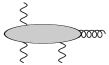
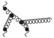
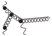
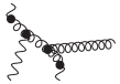
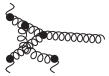
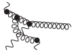
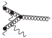
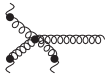
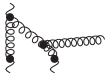
Figure 7: real NLO diagrams: the reggeized gluon + 2 reggeized gluon $\to$ gluon vertex

From Eq. (15), the momenta have the following Sudakov decomposition

$$p =p^{+}\frac{n^{-}}{2}+{\bm{p}} l =l^{-}\frac{n^{+}}{2}+{\bm{l}}$$

$$k =k^{-}\frac{n^{+}}{2}+{\bm{k}} q =q^{+}\frac{n^{-}}{2}+q^{-}\frac{n^{+}}{2}+{\bm{q}}\,.$$ (91)

With

$$i\mathcal{M}_{r^{*}g2r^{*}}^{ab_{1}b_{2}c} =\parbox{85.35826pt}{\includegraphics[width=71.13188pt]{BV.pdf}}$$ (92)

we obtain

$$a_{r^{*}2r^{*}g}^{ac}=\int\frac{dl^{-}}{8\pi}i\mathcal{M}_{r^{*}2r^{*}g}^{ab_{1}b_{2}c}P^{b_{1}b_{2}} =-\frac{g^{2}C_{a}\delta^{ac}{\bm{p}}^{2}}{(N_{c}^{2}-1)^{1/2}}\left[2\frac{{\bm{p}}\cdot{\bm{\epsilon}}}{{\bm{p}}^{2}}-\frac{({\bm{p}}-{\bm{l}}_{1})\cdot{\bm{\epsilon}}}{({\bm{p}}-{\bm{l}}_{1})^{2}}+\frac{({\bm{q}}-{\bm{l}}_{1})\cdot{\bm{\epsilon}}}{({\bm{q}}-{\bm{l}}_{1})^{2}}\right],$$ (93)

where we used the polarization vectors of Eqs. (27), (28) for the real gluon with momentum $q$. Absorbing also half of the propagators of the internal reggeized gluon line into the RP2R vertex, we obtain at cross-section level for the ‘$RG2R$’-vertex

$$V_{r^{*}2r^{*}g}({\bm{k}},{\bm{q}}) d\ln q^{+}=\int\frac{dk^{-}d{p}^{+}}{(2\pi)^{2}(4\pi)^{2+2\epsilon}}\left(\frac{1/4}{{\bm{p}}^{2}}\right)P^{aa^{\prime}}\left|a_{r^{*}2r^{*}g}^{ac}\left(a_{r^{*}2r^{*}g}^{a^{\prime}c}\right)^{*}\right|d\Phi^{(1)}$$

$$= \frac{\alpha_{s}^{2}C_{a}^{2}{\bm{p}}^{2}}{2\pi\mu^{4\epsilon}\Gamma^{2}(1-\epsilon)(N_{c}^{2}-1)^{3/2}}\left[\frac{{\bm{p}}}{{\bm{p}}^{2}}-\frac{1}{2}\frac{({\bm{p}}-{\bm{l}}_{1})}{({\bm{p}}-{\bm{l}}_{1})^{2}}+\frac{1}{2}\frac{({\bm{q}}-{\bm{l}}_{1})}{({\bm{q}}-{\bm{l}}_{1})^{2}}\right]$$

$$\hskip 142.26378pt\cdot\left[\frac{{\bm{p}}}{{\bm{p}}^{2}}-\frac{1}{2}\frac{({\bm{p}}-{\bm{l}}_{2})}{({\bm{p}}-{\bm{l}}_{2})^{2}}+\frac{1}{2}\frac{({\bm{q}}-{\bm{l}}_{2})}{({\bm{q}}-{\bm{l}}_{2})^{2}}\right]d\ln q^{+}.$$ (94)

Here the 1-particle phase space has been taken to be

$$d\Phi^{(1)} =2\pi\delta(p^{+}k^{-}-{\bm{q}}^{2}).$$ (95)

Momentum conservation ${\bm{k}}={\bm{q}}+{\bm{p}}$ is also implied. For the coupling of a single reggeized gluon to a quark, we obtain at cross-section level

$$\tilde{h}^{(0)}({\bm{p}}^{2}) =\frac{1}{2}\sum_{\text{spin}}\frac{1}{N_{c}}\sum_{\text{color}}\int\frac{dp^{-}}{4p_{a}^{+}(2\pi)^{2+\epsilon}{\bm{p}}^{2}}P^{aa^{\prime}}\left|\mathcal{M}^{a}_{qr^{*}q}\left(\mathcal{M}^{a^{\prime}}_{qr^{*}q}\right)\right|^{2}d\Phi^{(1)}$$

$$=\frac{\alpha_{s}C_{f}2^{1+\epsilon}}{\Gamma(1-\epsilon)\mu^{2\epsilon}}\frac{C_{f}}{(N_{c}^{2}-1)^{1/2}{\bm{p}}^{2}},$$ (96)

where the 1-particle phase space is understood in this case as

$$d\Phi^{(1)} =2\pi\delta(p_{a}^{+}p^{-}-{\bm{p}}^{2}).$$ (97)

The complete high energy factorized cross-section for the process $q+2r^{*}\to q+g$ is given by

$$h^{(1),\text{fact.}}_{qg}d^{2+2\epsilon}{\bm{q}}\,d\ln q^{+} =\frac{1}{\pi^{1+\epsilon}}\tilde{h}^{(0)}({\bm{p}}^{2})\cdot V_{r^{*}2r^{*}g}({\bm{k}},{\bm{q}})d^{2+2\epsilon}{\bm{q}}\,d\ln q^{+}\,.$$ (98)

This provides the starting point for a resummation of logarithms in the partonic diffractive mass $\hat{M}_{X}^{2}=p_{a}^{+}k^{-}-{\bm{k}}^{2}$ build from the quark-gluon final state, see [31] for a related study.

Appendix B The inclusive Pomeron quark impact factor

In the following we determine the inclusive analog to the Mueller-Tang jet impact factor. To ease the calculation we take the cut-off on the diffractive mass in the limit $M_{X.\text{max}}^{2}\to\infty$. This is sufficient to have a simple analytic check on the exclusive Mueller-Tang impact factor determined in Sec. 5. The collinear counterterm reads in this case

$$\lim_{M_{X,\text{max}}^{2}\to\infty}\bigg{[}-\frac{\alpha_{s}}{2\pi}\left(\frac{1}{\epsilon}+\ln\frac{\mu_{F}^{2}}{\mu^{2}}\right)h^{(0)}_{g}C_{f}\int_{x_{0}}^{1}dxf_{q}\left(x,\mu_{F}^{2}\right)\left(2\ln\frac{x\cdot M_{X,\text{max}}^{2}}{{\bm{k}}^{2}}-\frac{3}{2}\right)\bigg{]}\;,$$ (99)

with $x_{0}={\bm{k}}^{2}/M^{2}_{X,\text{max}}$ The inclusive real corrections are at partonic level given by

$$h^{(1)}_{r,qg} =\lim_{M^{2}_{X,\text{max}}\to\infty}\int_{0}^{1}dz\int\frac{d^{2+2\epsilon}{\bm{q}}}{\pi^{1+\epsilon}}\theta\left(xM_{X,\text{max}}^{2}-\hat{M}_{X}^{2}-(1-x){\bm{k}}^{2}\right)$$

$$h^{(0)}\frac{\alpha_{s,\epsilon}}{2\pi}\frac{P_{gq}(z,\epsilon)}{\Gamma(1-\epsilon)\mu^{2\epsilon}}\bigg{[}C_{f}\left(\frac{{\bm{\Delta}}}{{\bm{\Delta}}^{2}}-\frac{{\bm{q}}}{{\bm{q}}^{2}}\right)-{C_{a}}\left(\frac{{\bm{p}}}{{\bm{p}}^{2}}+\frac{1}{2}\frac{{\bm{\Sigma}}_{1}}{{\bm{\Sigma}}_{1}^{2}}+\frac{1}{2}\frac{{\bm{\Upsilon}}_{1}}{{\bm{\Upsilon}}^{2}_{1}}\right)\bigg{]}$$

$$\hskip 113.81102pt\cdot\left[C_{f}\left(\frac{{\bm{\Delta}}}{{\bm{\Delta}}^{2}}-\frac{{\bm{q}}}{{\bm{q}}^{2}}\right)-{C_{a}}{}\left(\frac{{\bm{p}}}{{\bm{p}}^{2}}+\frac{1}{2}\frac{{\bm{\Sigma}}_{2}}{{\bm{\Sigma}}_{2}^{2}}+\frac{1}{2}\frac{{\bm{\Upsilon}}_{2}}{{\bm{\Upsilon}}^{2}_{2}}\right)\right],$$ (100)

with $\hat{M}_{X}^{2}=(p_{a}+k)^{2}=(p+q)^{2}$. The evaluation of the integrals over the terms proportional to $C_{f}^{2}$ is straightforward and yields

$$C_{f}I_{C_{f}^{2}}=\int_{0}^{1}dzP_{gq}(z,\epsilon)\int\frac{d^{2+2\epsilon}{\bm{q}}}{\pi^{1+\epsilon}}\frac{z^{2}{\bm{k}}^{2}}{{\bm{\Delta}}^{2}{\bm{q}}^{2}} =2C_{f}\frac{c_{\Gamma}(\epsilon)}{\epsilon}\bigg{[}\frac{1}{\epsilon}-\frac{3-2\epsilon}{2+4\epsilon}\bigg{]}({\bm{k}}^{2})^{\epsilon},$$ (101)

with

$$c_{\Gamma} =\frac{\Gamma(1-\epsilon)\Gamma^{2}(1+\epsilon)}{\Gamma(1+2\epsilon)}.$$ (102)

To evaluate the $C_{a}C_{f}$ contributions we make use of the integral $K_{2}^{\prime}$ defined and calculated up to order $\epsilon$ in [12], Eqs. (6.17) and (6.18),

$$K_{2}^{\prime}({\bm{q}}^{2},{\bm{\bm{q}}_{1}},{\bm{q}}_{2},\epsilon) =\int_{0}^{1}\frac{dz}{z}[2(1-z)+(1+\epsilon)z^{2}]\bigg{[}\bigg{(}\left\{\left[z{\bm{q}}_{1}+(1-z){\bm{q}}_{2}\right]^{2}\right\}^{\epsilon}-\left[(1-z)^{2}{\bm{q}}_{2}^{2}\right]^{\epsilon}\bigg{)}$$

$$\hskip 227.62204pt+({\bm{q}}_{2}\to{\bm{q}}_{1})\bigg{]}$$

$$=\epsilon\left[1+\frac{1}{2}\ln^{2}\left(\frac{{\bm{q}}_{1}^{2}}{{\bm{q}}_{2}^{2}}\right)-\frac{3}{2}\frac{({\bm{q}}_{1}^{2}-{\bm{q}}_{2}^{2})}{{\bm{q}}^{2}}\ln\left(\frac{{\bm{q}}_{1}^{2}}{{\bm{q}}_{2}^{2}}\right)-6\frac{|{\bm{q}}_{1}||{\bm{q}}_{2}|}{{\bm{q}}^{2}}\theta\sin\theta+8\psi^{\prime}(1)-2\theta^{2}\right],$$ (103)

with ${\bm{q}}={\bm{q}}_{1}-{\bm{q}}_{2}$ and $\theta$ the angle between ${\bm{q}}_{1}$ and ${\bm{q}}_{2}$ such that $|\theta|\leq\pi$. We further introduce a second integral

$$K_{2}^{{}^{\prime\prime}}({\bm{q}}_{1}^{2},\epsilon) =\int_{0}^{1}\frac{dz}{z}[2(1-z)+(1+\epsilon)z^{2}]\bigg{(}\left[(1-z)^{2}{\bm{q}}_{1}^{2}\right]^{\epsilon}-\left[{\bm{q}}_{1}^{2}\right]^{\epsilon}\bigg{)}$$

$$=\left[2\psi(1)-2\psi(3+2\epsilon)+\frac{6+13\epsilon+3\epsilon^{2}-2\epsilon^{3}}{(1+2\epsilon)(2+2\epsilon)}\right]\,.$$ (104)

We obtain

$$C_{f}I_{C_{f}C_{a}}(i)=\int_{0}^{1}dzP_{gq}(z,\epsilon)\int\frac{d^{2+2\epsilon}{\bm{q}}}{\pi^{1+\epsilon}} J_{1}({\bm{q}},{\bm{k}},{\bm{l}}_{i},z)=C_{f}\frac{c_{\Gamma}(\epsilon)}{2\epsilon}\bigg{[}2K_{2}^{{}^{\prime\prime}}({\bm{k}}^{2},\epsilon)-K_{2}^{{}^{\prime\prime}}({\bm{l}}_{i}^{2},\epsilon)$$

$$-K_{2}^{{}^{\prime\prime}}(({\bm{k}}-{\bm{l}}_{i})^{2},\epsilon)-K_{2}^{\prime}({\bm{k}}^{2},{\bm{l}_{i}}^{2},({\bm{l}_{i}}-{\bm{k}})^{2},\epsilon)\bigg{]},$$ (105)

where the angle $\theta$ in $K_{2}^{\prime}$ must be defined for vectors ${\bm{q}}_{1}={\bm{l}}_{i}$ and ${\bm{q}}_{2}={\bm{k}}-{\bm{l}}_{i}$ such that ${\bm{q}}_{1}-{\bm{q}}_{2}={\bm{k}}$ holds. For the terms proportional to $C_{a}^{2}$ we have for non-zero ${\bm{q}}^{2}$

$$z>\bar{z}_{0}=\frac{{\bm{q}}^{2}}{xM_{X,\text{max}}^{2}}.$$ (106)

The region $z\to 1$ is on the other hand already finite and the limit$M_{X,\text{max}}^{2}\to\infty$ can be taken immediately in this case. We obtain

$$\lim_{M_{X,\text{max}}^{2}\to\infty}\int\limits_{\bar{z}_{0}}^{1}P_{gq}(z,\epsilon) =2\ln\frac{xM_{X,\text{max}}^{2}}{{\bm{q}}^{2}}-\frac{3}{2}+\frac{\epsilon}{2}.$$ (107)

The appearance of a $\ln 1/{\bm{q}}^{2}$ in Eq. (107) requires a new integral which, up to order $\epsilon^{0}$, has been evaluated in [13], Eqs.(A1)-(A13). It reads

$$\tilde{I}_{1}\left({\bm{l}}^{2},{\bm{k}}^{2}_{1},{\bm{k}}_{2}^{2}\right) =\int\frac{d^{2+2\epsilon}{\bm{q}}}{\pi^{1+\epsilon}}\ln\left(\frac{1}{{\bm{q}}^{2}}\right)\frac{{\bm{l}}^{2}}{({\bm{q}}-{\bm{k}}_{1})^{2}({\bm{q}}-{\bm{k}}_{2})^{2}}$$

$$=\frac{\Gamma(1-\epsilon)\Gamma^{2}(1+\epsilon)}{\Gamma(1+2\epsilon)}\left({\bm{l}}^{2}\right)^{\epsilon}\bigg{\{}\frac{1}{\epsilon^{2}}\left[2-\left(\frac{{\bm{k}}_{1}^{2}}{{\bm{l}}^{2}}\right)^{\epsilon}-\left(\frac{{\bm{k}}_{2}^{2}}{{\bm{l}}^{2}}\right)^{\epsilon}\right]$$

$$\hskip 170.71652pt+4\psi^{\prime\prime}(1)\epsilon+\ln\frac{{\bm{k}}_{1}^{2}}{{\bm{l}}^{2}}\ln\frac{{\bm{k}}_{2}^{2}}{{\bm{l}}^{2}}+\frac{2}{\epsilon}\ln\frac{1}{{\bm{l}}^{2}}\bigg{\}},$$ (108)

with ${\bm{l}}^{2}=({\bm{k}}_{1}-{\bm{k}}_{2})^{2}$. Altogether we obtain

$$K_{A}\left(({\bm{k}}_{1}-{\bm{k}}_{2})^{2},{\bm{k}}_{1}^{2},{\bm{k}}_{2}^{2},x\cdot M_{X,\text{max}}^{2},\epsilon\right)=\bigg{[}\int_{\bar{z}_{0}}^{1}dzP_{gq}(z,\epsilon)\bigg{]}\frac{({\bm{k}}_{1}-{\bm{k}}_{2})^{2}}{({\bm{q}}-{\bm{k}}_{2})^{2}({\bm{q}}-{\bm{k}}_{1})^{2}}=c_{\Gamma}(\epsilon)$$

$$\quad\times\left[({\bm{k}}_{1}-{\bm{k}}_{2})^{2}\right]^{\epsilon}\bigg{\{}\frac{2}{\epsilon}\left[2\ln\frac{xM_{X,\text{max}}^{2}}{({\bm{k}}_{1}-{\bm{k}}_{2})^{2}}-\frac{3}{2}+\frac{\epsilon}{2}\right]+2\ln\frac{{\bm{k}}_{1}^{2}}{({\bm{k}}_{1}-{\bm{k}}_{2})^{2}}\ln\frac{{\bm{k}}_{2}^{2}}{({\bm{k}}_{1}-{\bm{k}}_{2})^{2}}$$

$$\qquad\qquad\qquad\qquad+\frac{2}{\epsilon^{2}}\bigg{[}2-\left(\frac{{\bm{k}}_{1}^{2}}{({\bm{k}}_{1}-{\bm{k}}_{2})^{2}}\right)^{\epsilon}-\left(\frac{{\bm{k}}_{2}^{2}}{({\bm{k}}_{1}-{\bm{k}}_{2})^{2}}\right)\bigg{]}+8\psi^{{}^{\prime\prime}}(1)\epsilon\bigg{\}}.$$ (109)

This integral then allows to express the $C_{a}^{2}$ contribution in the following way,

$$C_{f}I_{C_{a}^{2}} =\int_{\bar{z}_{0}}^{1}dzP_{gq}(z,\epsilon)J_{2}({\bm{q}},{\bm{k}},{\bm{l}}_{1},{\bm{l}}_{2})$$

$$= \frac{C_{f}}{4}\bigg{\{}K_{A}\left({\bm{l}}_{1}^{2},({\bm{l}}_{1}-{\bm{k}})^{2},{\bm{k}}^{2},xM_{X,\text{max}}^{2},\epsilon\right)+K_{A}\left(({\bm{l}}_{2}-{\bm{k}})^{2},{\bm{k}}^{2},{\bm{l}}_{2}^{2},xM_{X,\text{max}}^{2},\epsilon\right)$$

$$+K_{A}\left(({\bm{l}}_{1}-{\bm{k}})^{2},{\bm{l}}_{1}^{2},{\bm{k}}^{2},xM_{X,\text{max}}^{2},\epsilon\right)+K_{A}\left({\bm{l}}_{2}^{2},{\bm{k}}^{2},({\bm{l}}_{2}-{\bm{k}})^{2},xM_{X,\text{max}}^{2},\epsilon\right)$$

$$-\frac{1}{2}\bigg{[}K_{A}\left(({\bm{l}}_{1}-{\bm{l}}_{2})^{2},{\bm{l}}_{1}^{2},{\bm{l}}_{2}^{2},xM_{X,\text{max}}^{2},\epsilon\right)$$

$$\hskip 85.35826pt+K_{A}\left(({\bm{l}}_{1}+{\bm{l}}_{2}-{\bm{k}})^{2},({\bm{l}}_{1}-{\bm{k}})^{2},{\bm{l}}_{2}^{2},xM_{X,\text{max}}^{2},\epsilon\right)$$

$$+K_{A}\left(({\bm{l}}_{1}+{\bm{l}}_{2}-{\bm{k}})^{2},{\bm{l}}_{1}^{2},xM_{X,\text{max}}^{2},\epsilon\right)$$

$$\hskip 85.35826pt+K_{A}\left(({\bm{l}}_{1}-{\bm{l}}_{2})^{2},({\bm{l}}_{2}-{\bm{k}})^{2},({\bm{l}}_{1}-{\bm{k}})^{2},xM_{X,\text{max}}^{2},\epsilon\right)\bigg{]}\bigg{\}}.$$ (110)

Our final result then reads

$$h_{r}^{(1)} =h^{(0)}\frac{\alpha_{s}}{2\pi}\frac{\mu^{-2\epsilon}}{\Gamma(1-\epsilon)}\bigg{[}C_{f}^{3}I_{C_{f}^{2}}+C^{2}_{f}C_{a}I_{C_{f}C_{a}}(1)+C_{f}^{2}C_{a}I_{C_{f}C_{a}}(2)+C_{a}^{2}C_{f}I_{C_{a}^{2}}\bigg{]}.$$ (111)

Expanding in $\epsilon$ we find the following divergent terms

$$\frac{h_{r}^{(1)}}{h^{(0)}} =\alpha_{s}\frac{C^{3}_{f}}{\pi}\left(\frac{1}{\epsilon^{2}}-\frac{3}{2\epsilon}+\frac{\ln{\bm{k}}^{2}}{\epsilon}\right)+\frac{\alpha_{s}C_{a}^{2}C_{f}}{\pi\epsilon}\left(\ln\frac{xM_{X,\text{max}}^{2}}{{\bm{k}}^{2}}-\frac{3}{4}\right)+\mathcal{O}({\epsilon^{0}}).$$ (112)

Combining these terms with the virtual corrections in Eq. (5.1), including ultraviolet renormalization, and the collinear counterterm of Eq. (99), we find that all poles in $\epsilon$ cancel and the result is finite in the limit $\epsilon\to 0$.

References

- [1] A. H. Mueller and W.-K. Tang, Phys. Lett. B 284 (1992) 123.
- [2] L. N. Lipatov, Sov. J. Nucl. Phys. 23 (1976) 338; E. A. Kuraev, L. N. Lipatov, V. S. Fadin, Phys. Lett. B 60 (1975) 50; Sov. Phys. JETP 44 (1976) 443; Sov. Phys. JETP 45 (1977) 199; I. I. Balitsky, L. N. Lipatov, Sov. J. Nucl. Phys. 28 (1978) 822.
- [3] X.-C. Zheng, X.-G. Wu, S.-Q. Wang, J.-M. Shen and Q.-L. Zhang, JHEP 1310, 117 (2013) [arXiv:1308.2381 [hep-ph]]; F. Caporale, D. Yu. Ivanov and A. Papa, Eur. Phys. J. C 58, 1 (2008) [arXiv:0807.3231 [hep-ph]].
- [4] M. Hentschinski, A. Sabio Vera and C. Salas, Phys. Rev. Lett. 110, 041601 (2013) [arXiv:1209.1353 [hep-ph]]; Phys. Rev. D 87, 076005 (2013) [arXiv:1301.5283 [hep-ph]]; H. Kowalski, L. N. Lipatov, D. A. Ross and G. Watt, Eur. Phys. J. C 70 (2010) 983 [arXiv:1005.0355 [hep-ph]].
- [5] B. Ducloué, L. Szymanowski and S. Wallon, Phys. Rev. Lett. 112 (2014) 082003 [arXiv:1309.3229 [hep-ph]]; JHEP 1305, 096 (2013) [arXiv:1302.7012 [hep-ph]]; F. Caporale, B. Murdaca, A. Sabio Vera and C. Salas, Nucl. Phys. B 875, 134 (2013) [arXiv:1305.4620 [hep-ph]]; F. Caporale, D. Yu. Ivanov, B. Murdaca and A. Papa, Nucl. Phys. B 877, 73 (2013) [arXiv:1211.7225 [hep-ph]]; M. Angioni, G. Chachamis, J. D. Madrigal and A. Sabio Vera, Phys. Rev. Lett. 107 (2011) 191601 [arXiv:1106.6172 [hep-th]].
- [6] V. A. Khoze, A. D. Martin and M. G. Ryskin, Eur. Phys. J. C 73, 2503 (2013) [arXiv:1306.2149 [hep-ph]]; J. R. Forshaw, M. H. Seymour and A. Siodmok, JHEP 1211 (2012) 066 [arXiv:1206.6363 [hep-ph]]; R. M. Durán Delgado, J. R. Forshaw, S. Marzani and M. H. Seymour, JHEP 1108 (2011) 157 [arXiv:1107.2084 [hep-ph]]; J. R. Forshaw, A. Kyrieleis and M. H. Seymour, JHEP 0809 (2008) 128 [arXiv:0808.1269 [hep-ph]].
- [7] R. Enberg, G. Ingelman and L. Motyka, Phys. Lett. B 524, 273 (2002) [hep-ph/0111090].
- [8] L. Motyka, A. D. Martin and M. G. Ryskin, Phys. Lett. B 524, 107 (2002) [hep-ph/0110273].
- [9] F. Chevallier, O. Kepka, C. Marquet and C. Royon, Phys. Rev. D 79, 094019 (2009) [arXiv:0903.4598 [hep-ph]]; O. Kepka, C. Marquet and C. Royon, Phys. Rev. D 83 (2011) 034036 [arXiv:1012.3849 [hep-ph]].
- [10] V. S. Fadin and R. Fiore, Phys. Lett. B 440, 359 (1998) [hep-ph/9807472].
- [11] V. S. Fadin, R. Fiore and A. Papa, Nucl. Phys. B 865, 67 (2012) [arXiv:1206.5596 [hep-th]]; Phys. Lett. B 647, 179 (2007) [hep-ph/0701075]; Nucl. Phys. B 769, 108 (2007) [hep-ph/0612284]; V. S. Fadin, R. Fiore, A. V. Grabovsky and A. Papa, Nucl. Phys. B 784, 49 (2007) [arXiv:0705.1885 [hep-ph]].
- [12] V. S. Fadin, R. Fiore, M. I. Kotsky and A. Papa, Phys. Rev. D 61, 094006 (2000) [hep-ph/9908265].
- [13] V. S. Fadin, R. Fiore, M. I. Kotsky and A. Papa, Phys. Rev. D 61, 094005 (2000) [hep-ph/9908264].
- [14] L. N. Lipatov, Nucl. Phys. B 452 , 369 (1995) [hep-ph/9502308]; Phys. Rept. 286 (1997) 131 [hep-ph/9610276].
- [15] M. Hentschinski, J. D. Madrigal, B. Murdaca and A. Sabio Vera, The Gluon-Induced Mueller-Tang Jet Impact Factor at Next-to-Leading Order, to appear.
- [16] M. Hentschinski and A. Sabio Vera, Phys. Rev. D 85, 056006 (2012) [arXiv:1110.6741 [hep-ph]].
- [17] G. Chachamis, M. Hentschinski, J. D. Madrigal and A. Sabio Vera, Phys. Rev. D 87 (2013) 076009 [arXiv:1212.4992 [hep-ph]].
- [18] G. Chachamis, M. Hentschinski, J. D. Madrigal and A. Sabio Vera, Nucl. Phys. B 876, 453 (2013) [arXiv:1307.2591 [hep-ph]]; Nucl. Phys. B 861, 133 (2012) [arXiv:1202.0649 [hep-ph]].
- [19] M. Hentschinski, J. D. Madrigal, B. Murdaca and A. Sabio Vera, Phys. Lett. B, in press [DOI: 10.1016/j.physletb.2014.06.022] [arXiv:1404.2937 [hep-ph]].
- [20] C. Marquet, C. Royon, M. Trzebiński and R. Žlebčík, Phys. Rev. D 87, 3, 034010 (2013) [arXiv:1212.2059 [hep-ph]], C. Royon, arXiv:1310.4675 [hep-ph].
- [21] G. Chachamis, M. Hentschinski, J. D. Madrigal and A. Sabio Vera, Phys. Part. Nucl. 45, 788 (2014) [arXiv:1211.2050 [hep-ph]].
- [22] J. R. Forshaw, A. Kyrieleis and M. H. Seymour, JHEP 0506, 034 (2005) [hep-ph/0502086].
- [23] J. Bartels, Nucl. Phys. B 175, 365 (1980).
- [24] M. A. Braun, M. Yu. Salykin and M. I. Vyazovsky, Eur. Phys. J. C 72, 1864 (2012) [arXiv:1109.1340 [hep-ph]].
- [25] M. Hentschinski, PhD Thesis, arXiv:0908.2576 [hep-ph].
- [26] M. Hentschinski, Nucl. Phys. B 859, 129 (2012) [arXiv:1112.4509 [hep-ph]].
- [27] M. Ciafaloni, Phys. Lett. B 429, 363 (1998) [hep-ph/9801322].
- [28] J. Bartels, D. Colferai and G. P. Vacca, Eur. Phys. J. C 24, 83 (2002) [hep-ph/0112283].
- [29] F. Caporale, D. Yu. Ivanov, B. Murdaca, A. Papa and A. Perri, JHEP 1202, 101 (2012) [arXiv:1112.3752 [hep-ph]].
- [30] Z. Kunszt and D. E. Soper, Phys. Rev. D 46, 192 (1992). S. Catani and M. H. Seymour, Nucl. Phys. B 485, 291 (1997) [Erratum-ibid. B 510, 503 (1998)] [hep-ph/9605323].
- [31] J. Bartels and M. Wüsthoff, Z. Phys. C 66, 157 (1995), J. Bartels and M. Hentschinski, JHEP 0908 (2009) 103 [arXiv:0903.5464 [hep-ph]], J. Bartels, C. Ewerz, M. Hentschinski and A.-M. Mischler, JHEP 1005, 018 (2010) [arXiv:0912.4759 [hep-th]].