Gain-scheduled synchronization of parameter varying systems via relative $H_{\infty}$ consensus with application to synchronization of uncertain bilinear systems

Abstract

The paper considers a problem of consensus-based synchronization of uncertain parameter varying multi-agent systems. We present a method for constructing consensus-based synchronization protocol schedules for each agent to ensure it synchronizes with a reference parameter-varying system. The proposed protocol guarantees a specified level of $H_{\infty}$ transient consensus between the agents. The algorithm uses a consensus-preserving interpolation and produces continuous (in the scheduling parameter) coefficients for the protocol. An application to synchronization of uncertain bilinear systems is discussed.

1 Introduction

The problem of synchronization of complex dynamical networks of interconnected systems has received much attention recently in the context of multi-agent consensus [3, 6, 21, 1]. In particular, robust synchronisation of uncertain systems has gained attention recently [3, 17, 16], including the development of $H_{\infty}$ methodology for multi-agent consensus and synchronization. For instance, [17] considered an $H_{\infty}$ consensus synthesis of observer-based synchronization protocols for dynamical networks of uncertain agents and introduced the notion of $H_{\infty}$ disagreement between agents to quantify consensus performance of such networks. The model in [17] allows for a significant heterogeneity — not only the agents are subject to additive perturbations but they are also endowed with different sensing patterns.

The $H_{\infty}$ metric has been used as measure of robustness in a number of recent papers on multi-agent consensus and synchronization. The key distinction of the $H_{\infty}$ consensus-based approach of [17] (also see [20, 19]), which is also used in this paper, is its focus on disturbance attenuation to improve transient consensus. It was observed in [17] that $H_{\infty}$ optimization of consensus transients forces consensus objectives to become a priority for the agents, thus creating an essential prerequisite for synchronization.

This paper extends the approach of $H_{\infty}$ consensus performance proposed in [17] to systems which require a time-varying reference for synchronization. Time variations of systems coefficients pose an additional difficulty in addressing system robustness, since many standard robust control and filtering techniques developed for time-invariant systems are not directly transferable to time-varying systems. While in some situations the issue can be circumvented by restricting attention to a finite-horizon version of the problem [11], such an approach may not be suitable in synchronization problems. For instance, synchronization of nonlinear systems exhibiting chaotic behaviour requires the system to be continuously ‘locked’ into synchronous operation, otherwise even small discrepancies between trajectories will cause the system to lose synchrony in a very short time.

Gain-scheduling techniques provide an alternative to the finite-horizon analysis and synthesis of time-varying systems known as parameter-varying systems. Such systems, especially their linear versions termed linear parameter varying (LPV) systems, frequently arise in the control systems theory [10]. The controller design for such systems involves scheduling a number of controllers for different operating conditions. When the operating conditions are continuously monitored, a gain-scheduled controller can be designed by interpolating these controllers. This allows to avoid detrimental transients caused by controller switching. Stability and robustness preserving interpolation techniques for gain scheduling [13, 14, 22] provide a guarantee that the system governed by an interpolated controller remains stable while traversing between operating points.

Switching is particularly undesirable when the system employs high gains. Since the distributed estimation techniques in [17] were found to yield high gain observers in some cases, in this paper we develop the interpolation technique for gain-scheduled synchronization inspired by the stability and robustness preserving interpolation methods [12, 13, 22]. The proposed interpolated protocol preserves synchronization and $H_{\infty}$ consensus properties of the interpolants.

As is well known large variations in the system parameters usually lead to a conservative uncertainty model, resulting in infeasible $H_{\infty}$ design conditions or yielding controllers with unacceptably poor performance; the approach of $H_{\infty}$ disagreement optimization in [17] is not immune to this. The scheduling method proposed in this paper can alleviate this conservatism since it allows to consider multiple design points with smaller parameter variations at each point. This is a certain advantage of the proposed method over [17].

The paper further expands the preliminary results announced in [18] and applies them to the problem of synchronization for networks of uncertain single-input bilinear agents. In this problem, the bilinear ‘master’ system is assumed to be governed by a control signal known to each agent. Such a signal can be generated by the reference system and then made available to each agent, e.g., as in the ‘master-slave’ synchronization scheme [5, 8], or can be collectively generated by the network. We show that this signal can be used for protocol scheduling for each agent. As an illustration, synchronization of a network of chaotic oscillators is discussed.

The paper is organized as follows. In Section 2 we introduce the problem, first for a network of bilinear systems, and then for a more general class of parameter varying uncertain systems which include a globally Lipschitz nonlinearity. The main results of the paper are developed in Section 3, and the application of these results to synchronization of single-input bilinear systems is given in Section 4. The illustrating example is given in Section 5, followed by the Conclusions. The proofs of the results are collected in the Appendix.

Notation

$\mathbf{R}^{n}$ denotes the real Euclidean $n$-dimensional vector space, with the norm $\|x\|\triangleq(x^{\prime}x)^{1/2}$; the symbol ^′ denotes the transpose of a matrix or a vector, and $\otimes$ is the Kronecker product of two matrices. Given a symmetric $k\times k$ matrix $P$, $\lambda_{\min}(P)$ denotes the smallest eigenvalue of $P$. The symbol $\star$ in position $(k,l)$ of a block-partitioned matrix denotes the transpose of the $(l,k)$ block of the matrix. $\mathbf{1}_{p}$ is the vector in $\mathbf{R}^{p}$ with all unity components. We let $\|z\|_{P}\triangleq\sqrt{z^{\prime}Pz}$. $L_{2}[0,\infty)$ denotes the Lebesgue space of $\mathbf{R}^{k}$-valued vector-functions $z(\cdot)$, defined on $[0,\infty)$, with the norm $\|z\|_{2}\triangleq\left(\int_{0}^{\infty}\|z(t)\|^{2}dt\right)^{1/2}$.

2 Problem formulation

2.1 Motivating problem: synchronization of a network of single-input uncertain bilinear systems

Consider a collection of $N+1$ bilinear control systems-agents, labeled $0,\ldots,N$, each described by the equation

$$\dot{x_{i}}=(A_{0}+\rho(t)\Delta)x_{i}+u_{i}(t)+B_{2i}w_{i}(t),$$ (1)

$$x_{i}(0)=x_{i0},$$

where $x_{i}\in\mathbf{R}^{n}$ is the state of agent $i$, $u_{i}\in\mathbf{R}^{n}$ denotes the local control input to agent $i$ through which it can be interconnected with other agents in the network, and $w_{i}\in\mathbf{R}^{r_{i}}$ is the disturbance. $A_{0}$, $\Delta$ are constant matrices. Also, $\rho:[0,\infty)\to\Gamma\triangleq[\rho^{\mathrm{min}},\rho^{\mathrm{max}}]\subset\mathbf{R}$ is a continuous differentiable signal known to all agents.

The signal $\rho(t)$ can be thought of as control steering the entire network to a desired behavior. One way to achieve this is to design such a control signal $\rho$ for one of the agents, and then control all other agents to track the leader; cf. [1]. Without loss of generality, suppose agent 0 is selected to be the leader. To distinguish this agent from other agents $i$, $i=1,\ldots,N$, its state is denoted $x$, and its evolution is described as

$$\dot{x}=(A_{0}+\rho(t)\Delta)x+B_{20}w_{0}(t),\quad x(0)=x_{0}.$$ (2)

The system (2) is bilinear and is governed by the common control signal $\rho(t)$. However for the leader we let $u_{0}=0$, to ensure its dynamics are not affected by the network.

Remark 1.

According to one of the original viewpoints on the gain scheduled design motivated by the objective of governing the system to an a priori known trajectory [10], $\rho(t)$ is assumed to be known to all agents. It can be either given (e.g., the desired heading for the formation) [10], or can be computed by each agent in the network, e.g., using nearest neighbours rules [9].

Suppose each agent (1) receives broadcast signals $y_{i}$, $v_{ij}$ from the reference plant and its neighbours $j$ (cf. [19]):

$$y_{i}=C_{2i}x+D_{2i}w_{i},\quad v_{ij}=H_{ij}x_{j}+G_{ij}w_{ij},$$ (3)

here $w_{ij}$ are disturbances affecting the communication between $j$ and $i$. We wish to design a protocol for interconnecting agents over a network, to ensure all of them track the leader. This problem is a special case of a more general synchronization problem introduced in the next section.

2.2 Synchronization problem for a network of parameter-varying agents

Consider a fixed directed graph $\mathbf{G}=(\mathbf{V},\mathbf{E})$; $\mathbf{V}$, $\mathbf{E}$ are the set of vertices and the set of edges (i.e, the subset of the set $\mathbf{V}\times\mathbf{V}$), respectively. Without loss of generality, we let $\mathbf{V}=\{1,2,\ldots,N\}$. The notation $(j,i)$ will denote the edge of the graph originating at node $j$ and ending at node $i$. It is assumed that the graph $\mathbf{G}$ has no self-loops, $(i,i)\not\in\mathbf{E}$.

For each $i\in\mathbf{V}$, let $\mathbf{V}_{i}=\{j:(j,i)\in\mathbf{E}\}$ be the set of nodes supplying information to node $i$, termed as the neighbourhood of node $i$. The cardinality of $\mathbf{V}_{i}$ is the in-degree of node $i$ and is denoted $p_{i}$; i.e., $p_{i}$ is equal to the number of incoming edges for node $i$. Also, $q_{i}$ will denote the number of outgoing edges for node $i$, known as the out-degree of node $i$. According to Proposition 1 in [17], the attention is restricted to weakly connected graphs.

Consider a multi-agent system, consisting of a parameter varying nonlinear reference system

$$\dot{x}=A(\rho(t))x+B_{1}\phi(x)+B_{20}w_{0}(t),\quad x(0)=x_{0},$$ (4)

and $N$ parameter varying nonlinear dynamical agents,

$$\dot{x_{i}}=A(\rho(t))x_{i}+B_{1}\phi(x_{i})+u_{i}(t)+B_{2i}w_{i}(t),$$ (5)

$$x_{i}(0)=x_{i0}.$$

Here the variables $x,x_{i},u_{i},w_{i}$ have the same meaning as in Section 2.1, and $\rho(t)$ is the time-varying parameter available to all agents, described previously. The matrix-valued function $A(\cdot)$ is assumed to be continuous on the interval $\Gamma$. Also, the function $\phi(x):\mathbf{R}^{n}\to\mathbf{R}^{l}$ satisfies the global Lipschitz condition

$$\|\phi(x_{1})-\phi(x_{2})\|^{2}\leq(x_{1}-x_{2})^{\prime}R(x_{1}-x_{2}),\quad\forall x_{1},x_{2}\in\mathbf{R}^{n};$$ (6)

where $R=R^{\prime}\geq 0$. The system (4) and the agents model (5) include the bilinear systems (2) and (1) considered in Section 2.1 as special cases, where $A(\rho)=A_{0}+\rho\Delta$ and $\phi(x)\equiv 0$. Also, we let $R=0$ in this special case.

As stated in Section 2.1, we assume that direct measurements of the reference plant (4) are not available, and each agent (5) must rely on broadcast signals from the reference plant and its neighbours defined in (3). It is assumed that $w_{0}$, $w_{i}(\cdot),w_{ij}(\cdot)\in L_{2}[0,\infty)$, $i,j=1,\ldots,N$. Also, we assume that $E_{2i}=D_{2i}D_{2i}^{\prime}>0$, $F_{ij}=G_{ij}G_{ij}^{\prime}>0$ for all $i$.

Consider the following consensus-based protocol for interconnecting the agents over the graph $\mathbf{G}$:

$$u_{i}(t) = L_{i}(\rho(t))(y_{i}-C_{2i}x_{i})$$ (7)

$$+\sum_{j\in\mathbf{V}_{i}}K_{ij}(\rho(t))(v_{ij}-H_{ij}x_{i}),$$

where $L_{i}(\cdot)$, $K_{ij}(\cdot)$ are matrix-valued gain functions to be determined. The synchronization problem in this paper is to determine the interconnection feedback gains $K_{ij}(\cdot)$ and observer gains $L_{i}(\cdot)$ such that $x_{i}(t)\to x(t)$ in the $L_{2}$ sense and asymptotically. This relates our approach to the distributed version of the observer-based synchronization problem; cf. [5]. As a distinctive feature of our approach, we aim to achieve synchronization while forcing the nodes to reach a guaranteed suboptimal level of relative $H_{\infty}$ disagreement, as stated in Definitions 1 and 2 given below. It is also worth noting that the agents in (5) have nonidentical measurement models which employ nonidentical matrices $C_{2i}$, $D_{2i}$. This is an important distinction between our model and those frequently used in the literature where all agents employ identical measurement models; e.g., see [3, 16].

As a measure of consensus between the agents consider the disagreement function (cf. [7])

$$\Psi_{\mathbf{G}}(\mathbf{x}) = \frac{1}{N}\sum_{i=1}^{N}\sum_{j\in\mathbf{V}_{i}}\|x_{j}-x_{i}\|^{2},\quad\mathbf{x}=[x_{1}^{\prime}~{}\ldots~{}x_{N}^{\prime}]^{\prime}.$$ (8)

In this paper, two synchronization problems are considered that utilize $\Psi_{\mathbf{G}}$ as the running cost of synchronization. In the first problem we are concerned with achieving synchronization with a guaranteed $H_{\infty}$ level of disagreement between the agents. In the second problem, a stronger version of disagreement performance is considered. It involves a penalty on the synchronization transient performance, additional to the penalty on the consensus transient performance.

Let $\mathbf{x}_{0}=[x_{10}^{\prime},\ldots,x_{N0}^{\prime}]^{\prime}$, and

$$\|(\mathbf{x}_{0},w_{0},\mathbf{w},\bar{\mathbf{w}})\|^{2} \triangleq \|\mathbf{1}_{n}\otimes x_{0}-\mathbf{x}_{0}\|^{2}_{P}+\|w_{0}\|_{2}^{2}$$

$$+\frac{1}{N}\sum_{i=1}^{N}\left(\|w_{i}\|_{2}^{2}+\sum_{j=1}^{N}\|w_{ij}(\cdot)\|^{2}_{2}\right),$$

where $P=P^{\prime}>0$ is a fixed matrix to be determined.

Definition 1.

The problem of weak robust synchronization is to determine continuous feedback control and interconnection gain schedules $L_{i}(\rho)$, $K_{i}(\rho)$, $\rho\in\Gamma$, for the protocol (7) to satisfy the following properties:

1. In the absence of uncertain perturbations, the interconnection of unperturbed systems describing evolution of the synchronization error dynamics of each agent $e_{i}\triangleq x-x_{i}$ must be exponentially stable. That is,

   $$\|e_{i}(t)\|^{2}\triangleq\|x_{i}(t)-x(t)\|^{2}\leq ce^{-\omega t},\quad(\exists c,\omega>0).$$

2. In the presence of uncertain perturbations, the protocol (7) must ensure a certain level of $H_{\infty}$ consensus performance in the following sense

   $$\sup_{\|(\mathbf{x}_{0},w_{0},\mathbf{w},\bar{\mathbf{w}})\|\neq 0}\frac{\int_{0}^{\infty}\Psi_{\mathbf{G}}(\mathbf{e}(t))dt}{\|(\mathbf{x}_{0},w_{0},\mathbf{w},\bar{\mathbf{w}})\|^{2}}\leq\gamma^{2}.$$ (9)

   Here, $\gamma>0$ is a given constant, and $\mathbf{e}=[e_{1}^{\prime},\ldots,e_{N}^{\prime}]^{\prime}$.

3. All agents synchronize asymptotically, i.e., for all $w_{0},w_{i},w_{ij}\in L_{2}[0,\infty)$,

   $$\lim_{t\to\infty}\sum_{i=1}^{N}\|x(t)-x_{i}(t)\|^{2}=0.$$ (10)

Definition 2.

Let $Q_{1},\ldots,Q_{N}$ be given symmetric positive definite matrices, and $Q\triangleq\mathrm{diag}[Q_{1},\ldots,Q_{N}]$. The problem of strong robust synchronization is to finding continuous feedback control and interconnection gain schedules $L_{i}(\rho)$, $K_{i}(\rho)$, $\rho\in\Gamma$, for the protocol (7) to satisfy conditions (i), (iii) of Definition 1, and the following condition, which replaces (9) in (ii):

$$\sup\frac{\int_{0}^{\infty}\left(\frac{1}{N}\mathbf{e}(t)^{\prime}Q\mathbf{e}(t)+\Psi_{\mathbf{G}}(\mathbf{e}(t))\right)dt}{\|(\mathbf{x}_{0},w_{0},\mathbf{w},\bar{\mathbf{w}})\|^{2}}\leq\gamma^{2}.$$ (11)

where the $\sup$ is over the set $\{\|(\mathbf{x}_{0},w_{0},\mathbf{w},\bar{\mathbf{w}})\|\neq 0\}$.

Condition (11) guarantees $H_{\infty}$ filtering performance $\int_{0}^{\infty}\mathbf{e}(t)^{\prime}Q\mathbf{e}(t)dt\leq\gamma^{2}N\|(\mathbf{x}_{0},w_{0},\mathbf{w},\bar{\mathbf{w}})\|^{2}$, which is not guaranteed by conditions in Definition 1. Hence the term strong synchronization. Also, the novel aspect in both definitions concerns the asymptotic synchronization property in condition (iii); an $L_{2}$ convergence was claimed in [17].

3 The main results

The derivation of the main result of the paper will proceed in several steps, following the general scheme of stability and robustness preserving interpolated gain-scheduling [12, 14, 22]. First, we revisit the results in [17] for a fixed parameter case and a more general class of agents under consideration in this paper. Recall that in [17], an ideal communication between the agents was assumed, whereas in this paper we allow for a more general situation where the messages between the agents are subject to disturbance. Next, based on this extension, a synchronization result will be established for a class of parameter-varying systems with a small-scale parameter variation. While technically simple, this extension will serve as the basis for the derivation of interpolated feedback schedules for a more general class of parameter-varying systems with bounded rate of parameter variations, which is the main result of this paper.

3.1 Synchronization of fixed parameter systems

Let us fix $\rho\in\Gamma$ and consider the fixed parameter version of the uncertain reference system (4),

$$\dot{x}=A(\rho)x+B_{1}\phi(x)+B_{20}w_{0}+\psi(t,x),\quad x(0)=x_{0},$$ (12)

and the corresponding $N$ uncertain fixed-parameter dynamical agents

$$\dot{x_{i}} = A(\rho)x_{i}+B_{1}\phi(x_{i})+\psi(t,x_{i})$$ (13)

$$+u_{i}(t)+B_{2i}w_{i}(t),\qquad x_{i}(0)=x_{i0}.$$

Compared with (5), we have introduced an additional uncertainty term to the reference plant and the equations of agents’ dynamics. The motivation for this will become clear later, when we will consider small parameter variations in the agents and the reference plant. Such small variations can be treated as an additional norm-bounded uncertainty, capturing the mismatch between fixed system parameters used in the protocol design, and the true system parameters. It will be shown that the size of this mismatch can be characterized in terms of a uniform norm bound condition, such as

$$\|\psi(t,x)-\psi(t,x_{i})\|^{2} \leq \alpha^{2}\|e_{i}\|^{2},$$ (14)

where $\alpha>0$ is a constant.

We now present a sufficient condition for the existence of a fixed parameter version of the protocol (7) which ensures that the fixed parameter systems (13) achieve strong synchronization. Given constants $\delta_{i}>0$ and matrices $Q_{i}=Q_{i}^{\prime}>0$, $i=1,\ldots,N$, introduce the following coupled Linear Matrix Inequalities (LMIs) in scalar variables $\tau_{i}>0$, $\theta_{i}>0$ and matrix variables $X_{i}=X_{i}^{\prime}>0$:

$$\left[\begin{array}[]{ccc}S_{i}(\rho)+\tau_{i}R+\theta_{i}\alpha^{2}I&\star&\star\\ T_{i}^{\prime}&-\Upsilon_{i}&*\\ X_{i}&0&-\theta_{i}I\end{array}\right]<0,$$ (18)

where $T_{i}=\left[\begin{array}[]{cccc}X_{i}B_{20}&X_{i}B_{2}(I-D_{2i}^{\prime}E_{i}^{-1}D_{2i})&X_{i}B_{1}&\Xi_{i}\end{array}\right],$

$$S_{i}(\rho)\triangleq X_{i}(A(\rho)+\delta_{i}I+B_{2i}D_{2i}^{\prime}E_{2i}^{-1}C_{2i})$$

$$\phantom{S_{i}(\rho)}+(A(\rho)+\delta_{i}I+B_{2i}D_{2i}^{\prime}E_{2i}^{-1}C_{2i})^{\prime}X_{i}+(p_{i}+q_{i})I$$

$$\phantom{S_{i}(\rho)}-\gamma^{2}C_{2i}^{\prime}E_{2i}^{-1}C_{2i}-\gamma^{2}\sum_{j\in\mathbf{V}_{i}}H_{ij}^{\prime}F_{ij}^{-1}H_{ij}+Q_{i},$$

$$\Xi_{i}=\left[\begin{array}[]{ccc}\gamma^{2}H_{ij_{1}}^{\prime}F_{ij_{1}}^{-1}H_{ij_{1}}\!-I&\ldots&\gamma^{2}H_{ij_{p_{i}}}^{\prime}F_{ij_{p_{i}}}^{-1}H_{ij_{p_{i}}}\!-I\end{array}\right],$$ (20)

$$\Upsilon_{i}=\mathrm{diag}\left[\gamma^{2}I,~{}\gamma^{2}I,~{}\tau_{i}I,~{}Z_{i}\right],$$

$$Z_{i}=\mathrm{diag}\left[\frac{2\delta_{j_{1}}}{q_{j_{1}}+1}X_{j_{1}},~{}\ldots,~{}\frac{2\delta_{j_{p_{i}}}}{q_{j_{p_{i}}}+1}X_{j_{p_{i}}}\right],$$ (21)

$j_{1},\ldots,j_{p_{i}}$ are the elements of the neighbourhood set $\mathbf{V}_{i}$.

Lemma 1.

Let $\rho\in\Gamma$ be given and fixed. Suppose the graph $\mathbf{G}$, the matrices $Q_{i}=Q_{i}^{\prime}>0$ and the constants $\gamma>0$ and $\delta_{i}>0$ are such that the coupled LMIs (18) corresponding to the given $\rho$ are feasible. Consider a collection of feasible triples $(\tau_{i,\rho},\theta_{i,\rho},X_{i,\rho})$, $i=1,\ldots,N$, and define

$$K_{ij}(\rho) = \gamma^{2}X_{i,\rho}^{-1}H_{ij}^{\prime}F_{ij}^{-1},$$ (22)

$$L_{i}(\rho) = (\gamma^{2}X_{i,\rho}^{-1}C_{2i}^{\prime}-B_{2i}D_{2i}^{\prime})E_{2i}^{-1}.$$ (23)

The network of fixed parameter agents (13), equipped with the protocols (7) with the coefficients defined in (22), (23) solves the fixed parameter version of the strong robust synchronization problem in Definition 2, with $\rho(t)\equiv\rho$. The matrix $P$ in condition (11) corresponding to this solution is $P=\mathrm{diag}[\frac{1}{N}X_{i,\rho}]$.

The proof of this lemma, as well as the proofs of other results in this paper is given in the Appendix. The main idea of the proof is to show that the interconnected system describing dynamics of the synchronization errors associated with the reference (12) and the multi-agent system (13) has the properties of vector dissipativity [2] with respect to the vector storage function $[V_{1}(e_{1})~{}\ldots~{}V_{N}(e_{N})]^{\prime}$, $V_{i}(e_{i})=e_{i}^{\prime}X_{i,\rho}e_{i}$, and a suitably defined vector of supply rates.

Remark 2.

The LMIs in (18) are coupled for neighbouring agents. In [17] we noted that in principle LMIs of this type can be solved in a distributed manner. Due to space limitation, we refer the reader to [17] for details.

3.2 Synchronization under small parameter variations

The protocol (7) defined in the previous section for the fixed parameter network can be used in the derivation of a synchronization protocol for the parameter varying multi-agent system (4), (5), provided parameter variations are sufficiently small, i.e. $\rho(t)\approx\rho^{0}$ $\forall t\geq 0$. In this case small variations of the matrix $A(\cdot)$ can be treated as parameter mismatch disturbances, and the parameter varying system (5) and the reference (4) can be regarded as a perturbation of a corresponding fixed-parameter system. To formalize this observation, let us fix $\rho^{0}\in\Gamma$, and define

$$\psi(t,x)=(A(\rho(t))-A(\rho^{0}))x.$$

The robust fixed parameter synchronization protocol of the form (7) can now be designed based on the representation (12), (13) using Lemma 1. This leads to the following result about synchronization of the system (4), (5) under small parameter variations.

Theorem 1.

Let $\rho^{0}\in\Gamma$ be fixed. Suppose that for all $t>0$

$$(A(\rho(t))-A(\rho^{0}))^{\prime}(A(\rho(t))-A(\rho^{0}))\leq\alpha^{2}I.$$ (24)

Suppose the graph $\mathbf{G}$ and the constants $\gamma>0$ and $\delta_{i}>0$ are such that the coupled LMIs (18) with $\rho=\rho^{0}$ are feasible, and let $(\tau_{i,\rho^{0}},\theta_{i,\rho^{0}},X_{i,\rho^{0}})$, be a corresponding collection of feasible triples, $i=1,\ldots,N$. Then the network of agents (5) equipped with the protocols (7), (22), (23), where $\rho=\rho^{0}$, solves the problem of strong robust synchronization in Definition 2. The matrix $P$ in conditions (9) and  (10) corresponding to this solution is $P=\mathrm{diag}[\frac{1}{N}X_{i,\rho^{0}}]$.

3.3 Disagreement gain preserving interpolation of synchronization protocols

Naturally, it may be difficult to cover the entire interval $\Gamma$ using a single condition (24) while ensuring that the coupled LMIs (18) are feasible for the selected $\alpha$. The idea behind the gain-scheduling approach in this paper is to cover the interval $\Gamma$ using smaller intervals for which conditions (24) and (18) hold simultaneously. First a collection of constants $\alpha_{k}>0$ and ‘grid points’ $\Gamma_{0}=\{\rho^{k},k=1,\ldots,M\}$ is selected so that for any $\rho\in\Gamma$ there exists at least one point $\rho^{k}$ with the property

$$(A(\rho)-A(\rho^{k}))^{\prime}(A(\rho)-A(\rho^{k}))\leq\alpha_{k}^{2}I.$$ (25)

Let $U_{k}$ be the largest connected neighbourhood of $\rho^{k}$ consisting of all $\rho\in\Gamma$ for which (25) holds. The grid points $\rho^{k}$ and the constants $\alpha_{k}$ must be selected so that $\Gamma\subseteq\cup_{k=1}^{M}U_{k}$. Next, using Lemma 1, we compute the synchronization protocol (7) for the uncertain parameter-varying agents plants (13) for each fixed $\rho^{k}$. The robustness properties of this protocol stated in Theorem 1 guarantee synchronization for every fixed $\rho\in\Gamma$. This property establishes an analog to the stability covering condition in [12].

Assuming that for every $\alpha=\alpha_{k}$ and $\rho=\rho^{k}$, $k=1,\ldots,M$, the LMIs (18) are feasible, the above procedure guarantees that for each fixed $\rho\in\Gamma$, a synchronization protocol (7) can be assigned to the system (5) by selecting one of the protocols corresponding to an index $k\in\{k:\rho\in U_{k}\}$. However, when applied to the parameter-varying system (4) directly, this procedure will result in the matrix-valued functions $L_{i}(\rho(t))$ and $K_{ij}(\rho(t))$ having jumps at the time instants when the trajectory of the parameter $\rho(t)$ exits the set $U_{k}$ and enters the set $U_{k+1}$. As a result, the control signals $u_{i}$ will become discontinuous and will generate transients that usually have an adverse effect on the system performance. To overcome these effects, we propose a continuous interpolation of the fixed-parameter synchronization protocols, following the interpolation approach in [12, 22, 14]. The aim of our interpolation technique is to preserve the property of interpolants to guarantee a desired level of the relative $H_{\infty}$ disagreement between the agents.

To explain the idea of the proposed interpolation, let us consider an arbitrary fixed $\rho\in\Gamma$, and the collection of constants $\alpha_{k}>0$, $k=1,\ldots,M$, and grid points $\Gamma_{0}$ discussed above. Since $\rho\in\Gamma$ is fixed, there must exist $k$ such that $\rho\in U_{k}$. Let $(\tau_{i,\rho^{k}},\theta_{i,\rho^{k}},X_{i,\rho^{k}})$, $i=1,\ldots,N$, be a feasible triple of the LMIs (18) corresponding to this $k$. The following lemma follows from (18) and (25) using the Schur complement.

Lemma 2.

Suppose (25) holds. The collection of matrices and constants $\{\tau_{i,\rho^{k}},X_{i,\rho^{k}},i=1,\ldots,N\}$, composed using a feasible solution of the LMI (18) corresponding to $\alpha=\alpha_{k}$, also satisfies the following coupled LMIs in $X_{i}=X_{i}^{\prime}>0$, $\tau_{i}>0$, $i=1,\ldots,N$:

$$\left[\begin{array}[]{cc}S_{i}(\rho)+\tau_{i}R&\star\\ T_{i}^{\prime}&-\Upsilon_{i}\end{array}\right]<0,$$ (28)

where $S_{i}(\rho)$, $T_{i}$ and $\Upsilon_{i}$ are the same as in (18).

We now define interpolated gains for the protocols (7), as follows. Suppose the collection of positive constants $\alpha_{k}$ and the grid points $\Gamma_{0}$ has the following properties:

$$(A(\rho)-A(\rho^{k}))^{\prime}(A(\rho)-A(\rho^{k}))\leq\alpha_{k}^{2}I,$$ (29)

$$\hskip 113.81102pt\mbox{if }\rho^{k}\leq\rho<\bar{\rho}^{k},$$

$$(A(\rho)-A(\rho^{k+1}))^{\prime}(A(\rho)-A(\rho^{k+1}))\leq\alpha_{k+1}^{2}I,$$ (30)

$$\hskip 113.81102pt\mbox{if }\underline{\rho}^{k+1}<\rho\leq\rho^{k+1},$$

where $\rho^{k}<\underline{\rho}^{k+1}<\bar{\rho}^{k}<\rho^{k+1}$. In particular, this implies that $[\underline{\rho}^{k+1},\bar{\rho}^{k}]\subset U_{k}\cap U_{k+1}$, and both (29) and (30) hold for $\rho\in[\underline{\rho}^{k+1},\bar{\rho}^{k}]$.

For every $\rho\in\Gamma$, select $k,k+1$ such that $\rho\in[\rho^{k},\rho^{k+1}]$, and define $\lambda=\frac{\bar{\rho}^{k}-\rho}{\bar{\rho}^{k}-\underline{\rho}^{k+1}}$,

$$X_{i,\rho} = \begin{cases}X_{i,\rho^{k}},&\rho\in[\rho^{k},\underline{\rho}^{k+1}],\\ X_{i,\lambda}\triangleq\lambda X_{i,\rho^{k}}+(1-\lambda)X_{i,\rho^{k+1}},\\ &\rho\in[\underline{\rho}^{k+1},\bar{\rho}^{k}],\\ X_{i,\rho^{k+1}},&\rho\in[\bar{\rho}^{k},\rho^{k+1}],\end{cases}$$ (31)

$$\tau_{i,\rho} = \begin{cases}\tau_{i,\rho^{k}},&\rho\in[\rho^{k},\underline{\rho}^{k+1}],\\ \tau_{i,\lambda}\triangleq\lambda\tau_{i,\rho^{k}}+(1-\lambda)\tau_{i,\rho^{k+1}},\\ &\rho\in[\underline{\rho}^{k+1},\bar{\rho}^{k}],\\ \tau_{i,\rho^{k+1}},&\rho\in[\bar{\rho}^{k},\rho^{k+1}],\end{cases}$$ (32)

$$K_{ij}(\rho) = \gamma^{2}X_{i,\rho}^{-1}H_{ij}^{\prime}F_{ij}^{-1}$$ (33)

$$L_{i}(\rho) = (\gamma^{2}X_{i,\rho}^{-1}C_{2i}^{\prime}-B_{2i}D_{2i}^{\prime})E_{2i}^{-1}.$$ (34)

Note that the matrix gains $K_{ij}$, $L_{i}$ defined above, are continuous and well defined functions on $\Gamma$, since $X_{i,\lambda}>0$ for all $\lambda\in[0,1]$, and hence $X_{i,\lambda}^{-1}$ is well defined.

The following theorem is the main result of the paper. Let $\bar{\Gamma}$ be the set consisting of all the corner points $\underline{\rho}^{k+1}$, $\bar{\rho}^{k}$, which lie inside $\Gamma$. Without loss of generality, we assume that $\rho(0)\not\in\bar{\Gamma}$, and that the set $\{t\colon\rho(t)\in\bar{\Gamma}\}$ has zero Lebesgue measure.

Theorem 2.

Suppose

$$\sup_{t\geq 0}|\dot{\rho}|\leq\min_{i}\left\{\lambda_{\min}(Q_{i})\left[\sup_{k}\frac{\left\|X_{i,\rho^{k+1}}-X_{i,\rho^{k}}\right\|}{\bar{\rho}^{k}-\underline{\rho}^{k+1}}\right]^{-1}\right\}.$$ (35)

Then the network of agents (5) equipped with the protocols (7), (33), (34), solves the weak robust synchronization problem in Definition 1. The matrix $P$ in condition (9) corresponding to this solution is $P=\mathrm{diag}[\frac{1}{N}X_{i,\rho(0)}]$.

If the inequality in (35) is replaced with a strict inequality, then strong synchronization can be established.

Corollary 1.

Suppose there exists $\eta\in[0,1)$ such that

$$\sup_{t\geq 0}|\dot{\rho}|\leq\eta\min_{i}\left\{\lambda_{\min}(Q_{i})\left[\sup_{k}\frac{\left\|X_{i,\rho^{k+1}}-X_{i,\rho^{k}}\right\|}{\bar{\rho}^{k}-\underline{\rho}^{k+1}}\right]^{-1}\right\}.$$ (36)

Then the network of agents (5) equipped with the protocols (7), (33), (34), solves the strong robust synchronization problem in Definition 2, with $Q$ in (11) replaced with $(1-\eta)Q$. The matrix $P$ is defined in the same way as in Theorem 2.

Remark 3.

It is worth noting that the variable $\gamma^{2}$ enters linearly in (18). This allows for optimization over $\gamma^{2}$. Such optimization can be carried out for each grid point $\rho^{k}$, and then the largest value out of obtained $\gamma^{2}_{k}$ should be selected. Maximization over $k$ is justified because if for a fixed $\rho=\rho_{k}$ the LMIs (18) admit a solution for $\gamma=\gamma_{k}$, then the same solution is feasible for these LMIs with any $\gamma>\gamma_{k}$.

4 Application to synchronization of single-input bilinear systems

We now apply the results of the previous section to the problem of synchronization of bilinear systems described in Section 2.1, where the matrix $A(\rho)$ is linear, $A(\rho)=A_{0}+\rho\Delta$, $A_{0}$, $\Delta$ are constant matrices. Owing to the affine structure of $A(\rho)$, the construction of the synchronization protocol can be further simplified, as presented below.

Let $\alpha>0$ and grid points $\Gamma_{0}=\{\rho^{k},k=1,\ldots,M\}$ be selected so that $|\rho^{k}-\rho^{k+1}|<\frac{\alpha}{\sigma(\Delta)},$ $\sigma(\Delta)$ is the largest singular value of $\Delta$, and $\rho^{1}\leq\rho^{\mathrm{min}}$, $\rho^{M}\geq\rho^{\mathrm{max}}$. Then the condition (25) trivially holds for any $\rho\in U_{k}=[\rho^{k-1},\rho^{k+1}]$, with $U_{1}=[\rho^{1},\rho^{2}]$, $U_{M}=[\rho^{M-1},\rho^{M}]$. Also, $\Gamma\subseteq\cup_{k=1}^{M}U_{k}$.

Suppose $\alpha$ is chosen so that for every $\alpha$ and $\rho=\rho^{k}$, $k=1,\ldots,M$, the LMIs (18) in the variables $(\theta_{i},X_{i})$ $X_{i}=X_{i}^{\prime}>0$, with $R_{i}=0$, are feasible. We allow for $R_{i}=0$ in this section since here we consider the special case $\phi(\cdot)\equiv 0$. The synchronization protocol (7) can then computed for each $\rho^{k}$ using Lemma 1, in which we let $R_{i}=0$. Furthermore, it is clear that for all $\rho\in\Gamma$, there exist two adjacent grid points $\rho^{k},\rho^{k+1}$ such that $\rho\in U_{k}\cap U_{k+1}$. Specifically, these $\rho^{k},\rho^{k+1}$ are the endpoints of the interval $[\rho^{k},\rho^{k+1}]$ to which $\rho$ belongs.

These considerations allow us to simplify the procedure of the previous section to construct interpolated gains for the protocol (7). For a $\rho$ such that $\rho\in[\rho^{k},\rho^{k+1}]$, let

$$X_{i,\rho} = \frac{\rho^{k+1}-\rho}{\rho^{k+1}-\rho^{k}}X_{i,k}+\frac{\rho-\rho^{k}}{\rho^{k+1}-\rho^{k}}X_{i,k+1}.$$ (37)

The following theorem specializes Theorem 2 and Corollary 1 to the problem of synchronization of bilinear systems.

Theorem 3.

Suppose condition (35), where $X_{i,k}$ are defined from (18) with $R_{i}=0$, holds. Then the network of agents (1) equipped with the protocols (7), (33), (34), solves the weak robust synchronization problem in Definition 1. Furthermore, if a stronger condition (36) holds, then the network of agents (1) equipped with the protocols (7), (33), (34), solves the strong robust synchronization problem in Definition 2, with $Q$ replaced with $(1-\eta)Q$. In both cases, the matrix $P$ in these definitions is obtained to be $P=\mathrm{diag}[\frac{1}{N}X_{i,\rho^{0}}]$.

5 Example: Master-slave synchronization of chaotic oscillators

To illustrate the results of the paper, consider the master-slave synchronization problem for a set of five 2nd-order bilinear systems with a so-called unified chaotic system [4] as a reference,

$$\dot{x}^{(1)} = (25\vartheta+10)(x^{(2)}-x^{(1)}),$$

$$\dot{x}^{(2)} = (28-35\vartheta)x^{(1)}+(29\vartheta-1)x^{(2)}-\rho(t)x^{(1)},$$

$$\dot{\rho} = -\frac{8+\vartheta}{3}\rho(t)+x^{(1)}x^{(2)}.$$ (38)

This system exhibits chaotic dynamics for all values of $\vartheta\in[0,1]$ [4]. Although the system is nonlinear, the first two equations can be regarded as a single-input bilinear system, with $\rho(t)$ interpreted as a control variable. This subsystem has the form (4) in which $w_{0}=0$, $\phi(x)=(\vartheta-\frac{1}{2})[x^{(1)}~{}x^{(2)}]^{\prime}$, and

$$A(\rho)=\left[\begin{array}[]{cc}-22.5&22.5\\ 10.5&13.5\end{array}\right]+\rho\left[\begin{array}[]{cc}0&0\\ -1&0\end{array}\right],\quad B_{1}=\left[\begin{array}[]{cc}-25&25\\ -35&29\end{array}\right].$$

To complete the analogy with (4), we randomly generated the matrix $B_{20}$ to be $B_{20}=[0.0806~{}0.0232]^{\prime}$, Clearly, (6) holds with $R=0.25I$ irrespective of $\vartheta$.

The network to be synchronized consists of controlled systems of the form (38). However, in accordance with the master-slave approach to synchronization, the signal $\rho$ is supplied by the master system (38), rather then being generated within the slave system. As a result, each slave system can be regarded as a 2nd-order system of the form (5) governed by the signal $\rho(t)$ generated by the reference system (38). We assume $B_{2i}=B_{20}$ for all agents.

It is easy to verify using simulations that if $u_{i}\equiv 0$, the agents systems do not synchronize to the reference system. This motivates us to introduce an additional control of the form (7) to achieve synchronization. For this example, a simple ring structure of the network was chosen, so that agent $i$ can receive information from agent $i-1$ and can forward its state to agent $i+1$. That is, $\mathbf{V}_{i}=\{i-1\}$ for $i=2,\ldots$, and $\mathbf{V}_{1}=\{N\}$. In this example, $N=5$.

Since the framework of the paper allows for synchronization via imperfect measurements and imperfect communication, we let $D_{2i}=0.01$, $G_{i,i-1}=0.2$ and randomly selected a set of matrices $C_{2i}$, $H_{i,i-1}$ to provide each agent with partial measurements of the reference plant and the partial information about the states of its neighbours. Also, the reference system (38) was simulated on the interval $[0,100]$, with the initial conditions $[0.3~{}0.3~{}20]^{\prime}$ and several values of $\vartheta$, to determine the bound on $|\dot{\rho}|$. It was found that on this time interval, $|\dot{\rho}|\leq 523.3044$ for the tested values of $\vartheta$.

To determine the interval $\Gamma$, we used the theoretical bound on trajectories of the Lorenz system $|\rho(t)-r|\leq\frac{b}{2\sqrt{b-1}}r$, where $r=28-35\vartheta>0$ [15]. Letting $\vartheta=0.5$ (the nominal system), we found $\Gamma=[0,56.2726]$. Next, 11 evenly spaced grid points were chosen as the set $\Gamma_{0}$, with $\rho^{0}=0$, $\rho^{11}=56.2726$, and the LMI optimization problem $\min\gamma^{2}$ subject to the LMI (18) was solved at each grid point, with $\delta=0.12$, $\alpha_{k}^{2}=32.3026$, and $Q=17\times I$, to obtain the matrices $X_{i,\rho^{k}}$. These parameters were chosen to ensure that conditions (29), (30) hold with $\bar{\rho}^{k}=\rho^{k+1}$ and $\underline{\rho}^{k+1}=\rho^{k}$. Clearly, $\rho(0)=20\not\in\Gamma_{0}$, as required in Theorem 2. Note that although the value of $\vartheta$ is assumed to be known in this example, we chose to use the matrix $R=0.25I$ which provides the upper bound on the Lipschitz constant of $\phi$ over $\vartheta$. This allows us to design the protocol (7) to be independent of the value of $\vartheta$, thus providing additional robustness.

We verified that the conditions of Theorem 2 were satisfied in this example, except for the rate bound condition (35). Unfortunately, this condition was difficult to satisfy in this example. Despite this, our simulations confirmed synchronization. This indicates that condition (35) is conservative.

The obtained matrices $X_{i,\rho^{k}}$ were used to schedule the coefficients for the protocol (7) according to (33) and (34). Here we implicitly used the observation that if the set of LMIs (18) admits a solution for $\gamma=\gamma_{k}$, then the same solution is feasible for these LMIs with any $\gamma>\gamma_{k}$; see Remark 3. Hence, the upper bound on the $H_{\infty}$ disagreement gain, guaranteed by the interpolated gain-scheduled synchronization protocol constructed in this example will be $\max_{k}\gamma_{k}^{2}=1.9729$.

To verify the design, the interconnected system was simulated on the time interval $[0,100]$. The plots of the errors $\|x-x_{i}\|$ for $\vartheta=0$ and $\vartheta=1$ are shown in Figure 1. It was observed in our simulations that all synchronization errors converged to 0, as was predicted by Theorem 2, even though the rate bound (35) failed to satisfy in this example. It is also worth noting that despite value of $\rho(t)$ varies substantially in this example, the error dynamics exhibit no sign of performance degrading transients while $\rho(t)$ varies. This reflects favourably on the proposed interpolated synchronization protocol.

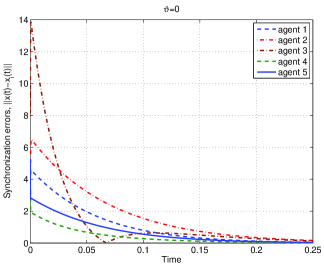
(a)

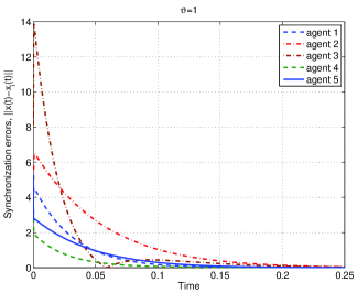
(b)

Figure 1: Synchronization errors $\|x-x_{i}\|$ versus time: (a) Interconnected systems, $\vartheta=0$; (b) Interconnected systems, $\vartheta=1$.

6 Conclusion

The paper has extended the gain-scheduling via interpolation technique to the class of synchronization problems for large-scale systems consisting of parameter varying agents with a Lipschitz continuous nonlinearity. The results have been applied to synchronization of multiagent network of bilinear systems.

It has been observed in our previous work [17] that the synchronization scheme proposed in that paper tends to use high gain observers to achieve synchronization. Large Lipschitz constants associated with system nonlinearities are likely to contribute to conservatism of the conditions in [17]. Consequently, this could be one reason for the algorithm [17] to yield high observer and interconnection gains. LPV modelling along the system trajectory may potentially reduce the size of the nonlinearity, and hence may lead to reduced gains required for synchronization. The results in this paper serve as a starting point for investigation into this hypothesis.

7 Appendix

7.1 Proof of Lemma 1

Consider a collection of interconnected systems describing dynamics of the synchronization errors associated with the system (12), (13) and the protocol (7),

$$\dot{e}_{i} = (A(\rho)-L_{i}(\rho)C_{2i})e_{i}+B_{1}\xi_{i}(t)+\zeta_{i}(t)$$ (39)

$$+ \sum_{j\in\mathbf{V}_{i}}K_{ij}(\rho)(H_{ij}(e_{j}-e_{i})-G_{ij}w_{ij})$$

$$+ +B_{20}w_{0}(t)-(B_{2i}+L_{i}(\rho)D_{2i}){w_{i}}(t),\qquad$$

$$e_{i}(0) = x_{0}-x_{i0},$$

$$\xi_{i}(t) = \phi(x(t))-\phi(x_{i}(t)),$$

$$\zeta_{i}(t) = \psi(t,x(t))-\psi(t,x_{i}(t)).$$ (40)

Using the constants $\tau_{i,\rho}>0$, $\theta_{i,\rho}>0$ and the matrix $X_{i,\rho}$ obtained from the LMIs (18), define $V_{i}(e_{i})=e_{i}^{\prime}X_{i,\rho}e_{i}$. In the same manner as in [17, 19], by completing the squares, one can establish that for all uncertainty signals $\xi_{i}(t)$, $\zeta_{i}(t)$ satisfying the constraints (6), (14), the following dissipation inequality holds

$$\mathbf{e}^{\prime}Q\mathbf{e}+N\Psi(\mathbf{e})+\dot{V}(\mathbf{e})\leq-\varepsilon V(\mathbf{e})$$ (41)

$$+\gamma^{2}\sum_{i=1}^{N}\left(\|w_{0}\|^{2}+\|w_{i}\|^{2}+\sum_{j\in\mathbf{V}_{i}}\|w_{ij}\|^{2}\right).$$

The statement of Lemma 1 now follows from (41). Indeed, properties (i) and (ii) of Definition 2 can be established using the same argument as that used to derive the statement of Theorem 1 in [17] from a similar dissipation inequality. Also, it follows from (41) and the condition $Q>0$ that $\mathbf{e}\in L_{2}[0,\infty)$. This implies that $\dot{\mathbf{e}}\in L_{2}[0,\infty)$. From the Cauchy-Schwartz inequality $\lim_{t\to\infty}\|\mathbf{e}(t)\|^{2}=2\lim_{t\to\infty}\int_{0}^{t}\mathbf{e}(t)^{\prime}\dot{\mathbf{e}}(t)dt$ exists. Since we have established that $\mathbf{e}\in L_{2}[0,\infty)$, this limit must be equal to 0. Thus, statement (iii) of Definition 2 holds as well. $\Box$

7.2 Proof of Theorem 2

Since the matrices $X_{i,\rho}$ are continuous and piecewise affine, they are differentiable on $\Gamma$ except at $\rho\in\bar{\Gamma}$. Using Lemma 6 of [13] and the definition of $X_{i,\rho}$ in (31), it follows that, given any $\epsilon>0$, there exists a continuously differentiable matrix function $Y_{i,\rho}$ defined on $\Gamma$, and a constant $\beta>0$ such that for any ‘corner’ point $c\in\bar{\Gamma}$,

$$\sup_{\rho\in\Gamma}\left\|Y_{i,\rho}-X_{i,\rho}\right\|<\epsilon,\quad\rho\in(c-\beta,c+\beta),$$ (42)

$$Y_{i,\rho}=X_{i,\rho},\quad\rho\not\in(c-\beta,c+\beta),$$ (43)

$$\sup_{\rho\in\Gamma}\left\|\frac{dY_{i,\rho}}{d\rho}\right\|\leq\sup_{k}\frac{\left\|X_{i,\rho^{k+1}}-X_{i,\rho^{k}}\right\|}{\bar{\rho}^{k}-\underline{\rho}^{k+1}}.$$ (44)

Note that the approximating matrices $Y_{i,\rho}$ can be chosen symmetric, since $X_{i,\rho}$ are symmetric. Also, if a sufficiently small $\epsilon>0$ is chosen, positive definite for all $\rho\in\Gamma$ matrices $Y_{i,\rho}$ can be selected.

Now suppose $\rho=\rho(t)\in[\rho^{k},\rho^{k+1}]$. Since both $(\tau_{i,\rho^{k}},X_{i,\rho^{k}})$ and $(\tau_{i,\rho^{k+1}},X_{i,\rho^{k+1}})$, $i=1,\ldots,N$, satisfy the LMIs (28), then due to the linearity of (28), $(\tau_{i,\rho},X_{i,\rho})$ are also feasible for the LMIs (28).

Let us now consider the synchronization errors for the system (4), (5), and the protocol (7) with the gains defined in (33), (34). It is straightforward to verify that the synchronization errors satisfy the equation (39) in which $\zeta_{i}\equiv 0$ and $\rho=\rho(t)$. Let us define the vector storage function candidate for this system, $V_{i}(e_{i},t)=e_{i}^{\prime}Y_{i,\rho(t)}e_{i}$. Also, let $\mathbf{w}^{i}=[w_{ij_{1}}^{\prime}~{}\ldots~{}w_{ij_{p_{i}}}^{\prime}]^{\prime}$. Since the inequality (28) is strict, the set $\Gamma$ is compact and $X_{i,\rho}$ is continuous with respect to $\rho$, then it is possible to choose a sufficiently small $\epsilon>0$ in (42) so that the following holds:

$$\frac{d}{dt}V_{i}(e_{i},t)=e_{i}^{\prime}\left(\frac{dY_{i,\rho(t)}}{dt}\right)e_{i}+2e_{i}^{\prime}Y_{i,\rho(t)}\dot{e}_{i}$$

$$<e_{i}^{\prime}\left(\frac{dY_{i,\rho(t)}}{dt}\right)e_{i}-e_{i}^{\prime}Q_{i}e_{i}-(p_{i}+q_{i})\|e_{i}\|^{2}$$

$$+2e_{i}^{\prime}\sum_{j\in\mathbf{V}_{i}}e_{j}-2\delta_{i}V_{i}(e_{i},t)+\sum_{j\in\mathbf{V}_{i}}\frac{2\delta_{j}}{q_{j}+1}V_{j}(e_{j},t)$$

$$+\gamma^{2}\|w_{0}\|^{2}+\gamma^{2}\|w_{i}\|^{2}+\gamma^{2}\sum_{j\in\mathbf{V}_{i}}\|w_{ij}\|^{2}.$$

We now observe that for $\rho(t)\in\Gamma\backslash\bar{\Gamma}$, it follows from (44) and (35) that $\left\|\frac{dY_{i,\rho(t)}}{dt}\right\|\leq\lambda_{\min}(Q).$ Therefore,

$$\frac{d}{dt}V_{i}(e_{i},t)<-(p_{i}+q_{i})\|e_{i}\|^{2}+2e_{i}^{\prime}\sum_{j\in\mathbf{V}_{i}}e_{j}$$ (45)

$$-2\delta_{i}V_{i}(e_{i},t)+\sum_{j\in\mathbf{V}_{i}}\frac{2\delta_{j}}{q_{j}+1}V_{j}(e_{j},t)$$

$$+\gamma^{2}\|w_{0}\|^{2}+\gamma^{2}\|w_{i}\|^{2}+\gamma^{2}\sum_{j\in\mathbf{V}_{i}}\|w_{ij}\|^{2}.$$

The remainder of the proof now follows using the same argument as that used in the proof of Lemma 1. $\Box$

7.3 Proof of Corollary 1

The proof is almost identical to the proof of Theorem 2. The only difference is to note that the stronger condition (36) will imply a stronger version of the vector dissipation inequality (45), with the additional term $-(1-\eta)e_{i}^{\prime}Q_{i}e_{i}$ on the right hand side.

References

- [1] H. F. Grip, T. Yang, A. Saberi, and A. A. Stoorvogel. Output synchronization for heterogeneous networks of non-introspective agents. Automatica, 48(10):2444–2453, 2012.
- [2] W. M. Haddad, V. Chellaboina, and S. G. Nersesov. Vector dissipativity theory and stability of feedback interconnections for large-scale non-linear dynamical systems. Int. J. Contr., 77(10):907–919, 2004.
- [3] Z. Li, Z. Duan, G. Chen, and L. Huang. Consensus of multiagent systems and synchronization of complex networks: A unified viewpoint. IEEE Trans. Circuits Syst. I: Regular Papers, 57:213–224, 2010.
- [4] J. Lü, G. Chen, D. Cheng, and S. C̆elikovský. Bridge the gap between the Lorenz system and the Chen system. International Journal of Bifurcation and Chaos, 12(12):2917–2926, 2002.
- [5] H. Nijmeijer and I.M.Y. Mareels. An observer looks at synchronization. IEEE Trans. Circuits Syst. I: Fundamental Theory and Applications, 44(10):882–890, Oct 1997.
- [6] R. Olfati-Saber, J.A. Fax, and R.M. Murray. Consensus and cooperation in networked multi-agent systems. Proceedings of the IEEE, 95(1):215–233, 2007.
- [7] R. Olfati-Saber and R. M. Murray. Consensus problems in networks of agents with switching topology and time-delays. IEEE Trans. Automat. Contr., 49:1520–1533, 2004.
- [8] L. M. Pecora and T. L. Carroll. Synchronization in chaotic systems. Phys. Rev. Lett., 64:821–824, 1990.
- [9] A.V. Savkin. Coordinated collective motion of groups of autonomous mobile robots: Analysis of Vicsek’s model. IEEE Trans. Automat. Contr., 49(6):981–982, June 2004.
- [10] J. S. Shamma and M. Athans. Analysis of gain scheduled control for nonlinear plants. IEEE Trans. Automat. Contr., 35(8):898–907, 1990.
- [11] B. Shen, Z. Wang, and Y. S. Hung. Distributed -consensus filtering in sensor networks with multiple missing measurements: The finite-horizon case. Automatica, 46(10):1682 – 1688, 2010.
- [12] D. J. Stilwell and W. J. Rugh. Interpolation of observer state feedback controllers for gain scheduling. IEEE Trans. Automat. Contr., 44(6):1225–1229, 1999.
- [13] D. J. Stilwell and W. J. Rugh. Stability preserving interpolation methods for the synthesis of gain scheduled controllers. Automatica, 36:665–671, 2000.
- [14] J. Stoustrup and M. Komareji. A parameterization of observer-ased controllers: Bumpless transfer by covariance interpolation. In Proc. American Contr. Conf., 2009., pages 1871–1875, 2009.
- [15] P. Swinnerton-Dyer. Bounds for trajectories of the Lorenz equations: an illustration of how to choose Liapunov functions. Physics Letters A, 281:161–167, 2001.
- [16] H. L. Trentelman, K. Takaba, and N. Monshizadeh. Robust synchronization of uncertain linear multi-agent systems. IEEE Trans. Automat. Contr., 58(6):1511–1523, 2013.
- [17] V. Ugrinovskii. Distributed robust filtering with consensus of estimates. Automatica, 47(1):1 – 13, 2011.
- [18] V. Ugrinovskii. Gain-scheduled synchronization of uncertain parameter varying systems via relative consensus. In Proc. Joint 50th IEEE CDC and ECC, pages 4251–4256, 2011.
- [19] V. Ugrinovskii. Distributed robust estimation over randomly switching networks using consensus. Automatica, 49(1):160–168, 2013.
- [20] V. Ugrinovskii and C. Langbort. Distributed consensus-based estimation of uncertain systems via dissipativity theory. IET Control Theory & App., 5(12):1458–1469, 2011.
- [21] T. Yang, A.A. Stoorvogel, and A. Saberi. Consensus for multi-agent systems — synchronization and regulation for complex networks. In Proc. American Contr. Conf., 2011, pages 5312–5317, 2011.
- [22] M. Yoon, V. Ugrinovskii, and M. Pszczel. Gain-scheduling of minimax optimal state-feedback controllers for uncertain linear parameter-varying systems. IEEE Trans. Automat. Contr., 52(2):311–317, 2007.