Quark ensembles with infinite correlation length

Abstract

By studying quark ensembles with infinite correlation length we formulate the quantum field theory model that, as we show, is exactly integrable and develops an instability of its standard vacuum ensemble (the Dirac sea). We argue such an instability is rooted in high ground state degeneracy (for ’realistic’ space-time dimensions) featuring a fairly specific form of energy distribution, and with the cutoff parameter going to infinity this inherent energy distribution becomes infinitely narrow and leads to large (unlimited) fluctuations. Analysing some possible vacuum ensembles such as the Dirac sea, neutral ensemble, color superconducting and BCS states we find out the strong arguments in favor of the BCS state as the ground state of color interacting quark ensemble.

I Introduction

Investigating quark ensembles with an infinite correlation length looks, from the view point of fundamental strong interactions existing between ensemble elements, like a purely academic task because the successful practical field theory (QCD) develops finite inherent scale as an abundant experience of phenomenological studies (and lattice QCD theory) gives an evidence. However, a true nature of these scale is still pretty uncertain problem fad . Here we are concerned with this problem by searching for the indicative consequences if the proper scale has already raised in a quantum field model. In our particular case of strongly interacting fields a model with ’infinite’ correlation length might be understood as one in which a size is determined by the characteristic vacuum box ($L\sim\Lambda^{-1}_{\mbox{\scriptsize{QCD}}}$). Moreover, we show, in what follows, the consideration of respective quark ensembles is getting essential technical simplification because the field theory models of our interest prove to be exactly integrable (in the sense by Thirring or Luttinger). This remarkable property of certain class of field theoretical models makes possible to proceed substantially beyond the perturbative approximation and plays role of great importance in understanding the principal problems of quantum field theory tir , bik . Besides, these models (called further as the KKB models) are also well-known and fruitful in the context of condensed matter physics kkb . We believe that studying the fundamental ensemble features is quite relevant and insightful to deal.

In fact, this feature of exact integrability has already been exploited mz at comparative analysis of the KKB and Nambu-Jona-Lasinio (NJL) models (both are the models of four-quark interaction). The model with ’infinite’ correlation length (KKB) provides also an interesting possibility to evaluate a role of quantum correlations only, i.e. at absence of a customary impact force intrinsic in classical dynamics or electrodynamics, what is quite inherent in studying a system of fermions and regarded as an exchange force atom , ato . Apparently, in this connection the problem of treating a system response to any external influence appears to be of special interest, for example, at analysing a system behavior in an external fields.

Ensemble action in which we are interested to investigate is presented as

$$S=\!\!\!\int dtd^{\mbox{\scriptsize{D}}}x\left[\bar{q}(i\hat{\partial}-m)q-\frac{\textstyle g}{\textstyle 2}~{}j^{a}_{\mu}\int d^{\mbox{\scriptsize{D}}}y~{}j^{\prime a}_{\mu}~{}F(x,y)\right].$$ (1)

Here $j^{a}_{\mu}=\bar{q}t^{a}\gamma_{\mu}q$ is a quark current with respective quark field operators $q$, $\bar{q}=q^{+}\gamma_{0}$ taken at the spatial point $x$ (the primed variables refer to the point $y$), $m$ is the current quark mass, $t^{a}=\lambda^{a}/2$ are the generators of the $SU(N_{c})$ color gauge group, $\mu=0,1,2,3,\dots D$ and $\hat{\partial}$ are the partial derivatives over time $t$ and coordinates $x$ spanned on the corresponding $\gamma$-matrices. The form of color interaction plays a significant role below, but we start our discussion with considering simpler abelian version. In two-dimensional (time and one spatial component, $D=1$) formulation such an ensemble corresponds to the Thirring or Luttinger model tir .

For the sake of simplicity the form-factor $F(x,y)$ is put to be translation invariant, $F(x,y)=F(x-y)$, and dimensionless with singling out a proper constant $g$. There is no any preferable spatial point in the ensemble with ’infinite’ correlation length (a force which is usually defined as a gradient of potential equals to zero), and it is just what we have in mind, while talking about absence of the customary force interaction. In principle, the form-factor could be taken as $F(x)=1$ and then the corresponding Fourier-transformation $\widetilde{F}(p)=\int d^{\mbox{\scriptsize{D}}}x~{}e^{ipx}F(x)=\delta(p)$ has a dimension $[F(p)]=L^{\mbox{\scriptsize{D}}}$. Concurrently, the dimension of quark fields comes about $[q]=L^{\mbox{\scriptsize{-D/2}}}$ and the coupling constant becomes dimensional $[g]=L^{-1}$. In what follows, we are dealing with the densities of ’measurable’ quantities, for example, an energy density ${\cal E}=E/L^{\mbox{\scriptsize{D}}}$ where $E$ is a total ensemble energy. In order to simplify the formulae we do not include the factors $L^{\mbox{\scriptsize{-D/2}}}$, in the definition of fermion fields, because they can be easily recast if necessary and as to the observables they are present via the corresponding factor of box volume $V=L^{\mbox{\scriptsize{D}}}$. What is more specific feature of interaction form considered concerns a formal absence of scattering, i.e. quark incoming momentum coincides with the quark outgoing momentum in the scattering process.

It should, perhaps, be recalled how, in principle, the effective form of interaction Eq. (1) could be obtained from QCD. It is assumed that quarks are under the influence of strong stochastic vacuum gluon fields. Then using the coarse-graining procedure for quark ensemble in quasistationary state we obtain product of interesting us quark currents associated with corresponding correlator (condensate) of the gluon field $\langle A^{a}_{\mu}A^{\prime b}_{\nu}\rangle$. In simplest form it is a color singlet. For sake of simplicity we restrict ourselves by a contact interaction in time (without retardation) and, hence, we do not include corresponding delta-function in time in the form of form-factor

$$\langle A^{a}_{\mu}A^{\prime b}_{\nu}\rangle=G~{}\delta^{ab}~{}\delta_{\mu\nu}~{}F({\mbox{\boldmath$x$}}-{\mbox{\boldmath$y$}})~{}.$$ (2)

Of course, there are another terms, spanned on the vector of relative distance $x-y$. It is clear that this simplest correlation function is only one of the fragments of corresponding ordered exponent and the four-fermion interaction is clearly accompanied by infinite number of multifermion vertices sim .

II Two-dimensional model

As a matter of fact, the two-dimensional version of model (1) is very well known and has been intensively studied for almost fifty years creating a fundamental basis for several areas in many-fermion physics research with the exciting claims of exact and complete integrability tir . Even nowadays this model is practically the only reliable instrument to describe (beyond the one-particle perturbation theory) a system response to an external influence. It seems curious, the case of correlations dominance, that we are interested in, was systematically excluded from consideration by applying the subtraction procedure, rejecting the contribution $\widetilde{F}(0)$. This variant was not thoroughly investigated because of various reasons, one of which is certainly too much simple.

If we limit ourselves to the abelian form of interaction (dropping the group generators $t^{a}$ out) it is possible to introduce a corresponding doublet of fields $q=(q_{1},q_{2})$ (instead of a full-fledged particle spin) for the two-dimensional model of Eq. (1). Then taking the $\gamma$-matrices in the form $\gamma_{0}=\sigma_{2}$, $\gamma_{1}=i\sigma_{1}$, where $\sigma_{1}$, $\sigma_{2}$ are the Pauli matrices we are able to transform the Lagrangian density to the form typical for models of Ref. tir

$${\cal L}=\bar{q}(i\hat{\partial}-m)q-g~{}(q^{+}_{1}q_{1}~{}q^{\prime+}_{2}q^{\prime}_{2}+q^{+}_{2}q_{2}~{}q^{\prime+}_{1}q^{\prime}_{1})~{}.$$ (3)

In order not to overload formulae we omit the integration over coordinate $y$, but keep it in mind putting the primes over the corresponding fermion fields in the proper places. The Hamiltonian density of system under consideration can be written down in the form

$${\cal H} = q^{+}_{1}~{}p~{}q_{1}-q^{+}_{2}~{}p~{}q_{2}+m(q^{+}_{1}q_{2}+q^{+}_{2}q_{1})+$$

$$+ g~{}(q^{+}_{1}q_{1}~{}q^{\prime+}_{2}q^{\prime}_{2}+q^{+}_{2}q_{2}~{}q^{\prime+}_{1}q^{\prime}_{1})~{},$$

where $p=i\partial_{x}$. Now following Thirring tir we introduce a reference vacuum state $|0)$ featuring the components of fermion fields as $q_{1x}|0)=q_{2x}|0)=0$. Since we consider a system into a finite size box, this condition is assumed to be valid in the corresponding discrete spatial points for the fermions with antiperiodic boundary conditions. First, we consider the system in the chiral limit ($m=0$), and define two Fourier transformed doublets of the Fermi field as

$$a_{ik}=\int dx~{}e^{-ikx}~{}q_{ix}~{},~{}~{}~{}q_{ix}=\int d\widetilde{k}~{}e^{ikx}~{}a_{ik}~{},$$ (5)

here $\widetilde{k}=k/(2\pi)$. When it is obvious from the context we omit the spatial point designation (for example, it is $x$ in the formula above). Then the free Hamiltonian density and the density of interaction term may be presented as

$${\cal H}_{0} = \sum\limits_{k}k~{}a^{+}_{1k}a_{1k}-\sum\limits_{k}k~{}a^{+}_{2k}a_{2k}~{},$$

$${\cal V} = 2g~{}\sum\limits_{k}a^{+}_{1k}a_{1k}\sum\limits_{l}a^{+}_{2l}a_{2l}~{},$$

(more precisely, the last expression should be symmetrized, but it does not play a significant role for further). Fermion anticommutation relations lead, as known tir , to the standard formulation of creation $a^{+}$ and annihilation $a$ operators with the standard anti-commutator valid $a^{+}a~{}+~{}aa^{+}=1$ (indices are omitted). It is easy to see that by the definition the reference state corresponds to the eigenstate of Hamiltonian $H=\int dx{\cal H}$, $H=H_{0}+V$ with zero eigenvalue $H|0)=0$, since $H_{0}|0)=0$, $V|0)=0$. However, the states of free Hamiltonian with negative energy (while working within the perturbation theory) give rise concern. We see from Eq. (II) that they are the states with negative momentum $a_{1k},k<0$ for particles of the first kind, and those are states with positive momentum $a_{2k},k>0$ for particles of the second kind. Usually, this problem is resolved by filling up the Dirac sea with particles of negative energy. Thus, we take an ansatz for ground state as follows

$$|0\rangle=\prod\limits_{k\geq-\Lambda}^{-P}a^{+}_{1k}\prod\limits_{l\geq P}^{\Lambda}a^{+}_{2l}~{}|0)~{}.$$ (7)

We introduce some auxiliary cutoff momentum $\Lambda$ in Eq. (7) that should eventually be going to infinity. Besides, we introduce a boundary momentum $P$, its meaning becomes clear below. The system ’charge’

$$Q=\int dx(q^{+}_{1}q_{1}+q^{+}_{2}q_{2})=\sum\limits_{k}(a^{+}_{1k}a_{1k}+a^{+}_{2k}a_{2k})$$

commutes with Hamiltonian $H$ and, hence, it is convenient to classify its eigenstates.

Then we have for the free Hamiltonian

$${\cal H}_{0}~{}|0\rangle=\left(\sum\limits_{-\Lambda}^{-P}k-\sum\limits^{\Lambda}_{P}k\right)|0\rangle~{},$$

and for the interaction term

$${\cal V}~{}|0\rangle=2gL(\Lambda-P)^{2}|0\rangle~{},$$

i.e. the energy density of such a Dirac sea looks like

$${\cal E}_{\mbox{\scriptsize{D}}}=-\Lambda(\Lambda+\widetilde{1})+P(P+\widetilde{1})+2gL(\Lambda-P)^{2}~{},$$ (8)

where by definition the momentum unity is $\widetilde{1}=2\pi/L$. It is interesting to notice that the parabola branches as a function of the cutoff $\Lambda$ for the coupling parameters $2gL>1$ change their directions, and the Dirac sea may have even a finite relative depth. Indeed, it makes sense to fill up the Dirac sea to some point $P$ where the Dirac sea is getting its minimal energy

$$\Lambda-P_{\mbox{\scriptsize{min}}}=\frac{\textstyle 1}{\textstyle 2}\frac{\textstyle 2\Lambda+\widetilde{1}}{\textstyle 2gL+\widetilde{1}},~{}{\cal E}_{\mbox{\scriptsize{min}}}=-\frac{\textstyle 1}{\textstyle 4}\frac{\textstyle 2\Lambda+\widetilde{1}}{\textstyle 2gL+\widetilde{1}}~{}(2\Lambda+\widetilde{1}).$$ (9)

Since we consider the system in a finite box it means an integer nearest to this value of $P_{\mbox{\scriptsize{min}}}$. Besides, it is also interesting that the ’vacuum’ state of Dirac sea is degenerate for almost all values of the coupling constant (there is an exact two-fold degeneracy for some discrete set of coupling constants) because the nearest integer either exceeds or is less than $P_{\mbox{\scriptsize{min}}}$. (It is clear that if this property is still valid for the multi-dimensional consideration, then the Dirac sea degeneracy is measured by the area of corresponding sphere, see below). We are talking about the relative depth of the Dirac sea in two-dimensional model because pointing the parameters $\Lambda$ and $P$, being consistently related, at infinity allows us to reach the unlimited low values of ${\cal E}_{\mbox{\scriptsize{D}}}$. Probably, it is rather the specific feature of two-dimensional model (see an analysis of multi-dimensional model below).

We have a standard picture of the Dirac sea at low values of coupling constant $gL\to 0$ but the boundary momentum $P$ becomes comparable with the cutoff scale $P\sim\Lambda/2$ already for the values of order $2gL\sim 1$. The excitations of such a Dirac sea are fairly curious. Adding or removing one particle of enormously huge momentum $\sim\Lambda/2$ results in a small energy increase $\sim d{\cal E}/dP|_{P=P_{\mbox{\scriptsize{min}}}}$ only, that, apparently, is inconsistent with observations. Amazingly, such states assume an existence of particle separation mechanism as the particles of one kind acquire mainly negative momenta unlike the particles of another kind possessing the positive ones. This behavior is rooted in a specific form of kinetic energy term of two-dimensional model in Eq. (II) if we consider the kinetic energy in the nonrelativistic approximation as a small deviation from the Fermi energy.

If we consider another example of ensemble with the same number of states of positive and negative momenta for both types of particles then there are the $L(\Lambda-P)$ particles of first type with positive momenta and the same number of particles of this type with negative momenta. Similar situation takes place for the particles of second type. Then the lowest energy for the particles of first type occurs if the states with negative momenta are collected from the sea bed (i.e. from cutoff momentum $\Lambda$). But the states with positive momenta fill the sea up starting from the lowest positive momenta, i.e. from unit. Similar picture takes place for the particles of second type with an obvious permutation of states with positive and negative momenta. Then we find the energy density as

$${\cal E}_{n}=-\Lambda(\Lambda+\widetilde{1})+P(P+\widetilde{1})+(\Lambda-P)(\Lambda-P+\widetilde{1})+$$

$$+4gL(\Lambda-P)^{2}=-(\Lambda-P)2P+4gL(\Lambda-P)^{2}~{}.$$ (10)

Comparing this result to Eq. (8) we see ’neutral’ ensemble energy density is simply controlled by the total number of particles, but we can show the ’absolute depth’ of its sea is poorly defined (tends to negative infinity). Then, overall impression of considering these particular examples suggests that the system properties appear to be dependent not only on the Hamiltonian but also on fixing the Hilbert space sector (symmetries) adequate to the problem considered fn . It seems to us the similar results could be hardly received (in one-particle approximation) by simply calculating the Hamiltonian determinant only. Below we compare these results to those obtained for the Thirring model with point-like interaction $F(x)=\delta(x)$.

In order to complete this simple analysis we consider our system beyond the chiral limit. Now the density of the free Hamiltonian takes the following form

$${\cal H}_{0}=\sum\limits_{k}k~{}(a^{+}_{1k}a_{1k}-a^{+}_{2k}a_{2k})+m(a^{+}_{1k}a_{2k}+a^{+}_{2k}a_{1k})~{}.$$ (11)

Diagonalizing this form with a canonical transformation to new creation and annihilation operators

$$\widetilde{A}_{1k}=\cos\varphi_{m}~{}a_{1k}+\sin\varphi_{m}~{}a_{2k}~{},$$

(12)

$$\widetilde{A}_{2k}=-\sin\varphi_{m}~{}a_{1k}+\cos\varphi_{m}~{}a_{2k}~{}.$$

where $\sin\theta_{m}=m/k$, $\cos\theta_{m}=k/k_{0}$, $k_{0}=(k^{2}+m^{2})^{1/2}$, $\theta_{m}=2\varphi_{m}$ we obtain the expansion of quark operators $q$ over annihilation operators (instead of Eq. (5)) as

$$q_{jx}=\sum\limits_{k}e^{ikx}~{}[\widetilde{U}_{k}(j)~{}\widetilde{A}_{1k}+\widetilde{V}_{k}(j)~{}\widetilde{A}_{2k}],$$ (13)

here $j=1,2$. At $k>0$ the spinors have the form

$$\widetilde{U}_{k}(1)=\left(\frac{\textstyle k_{0}+k}{\textstyle 2k_{0}}\right)^{1/2}\!\!\!\theta_{k},~{}\widetilde{U}_{k}(2)=\left(\frac{\textstyle k_{0}-k}{\textstyle 2k_{0}}\right)^{1/2}\!\!\!\theta_{k},$$

(14)

$$\widetilde{V}_{k}(1)=-\widetilde{U}_{k}(2)~{}~{},~{}\widetilde{V}_{k}(2)=\widetilde{U}_{k}(1)~{},$$

where $\theta_{k}$ is the theta-function ($\theta_{k}=1,k>0$, $\theta_{k}=0,k\leq 0$). Then, at $k<0$ we have similarly that

$$\widetilde{U}_{k}(1)=~{}~{}\left(\frac{\textstyle k_{0}+|k|}{\textstyle 2k_{0}}\right)^{1/2}\!\!\!\theta_{-k},~{}\widetilde{U}_{k}(2)=-\left(\frac{\textstyle k_{0}-k|}{\textstyle 2k_{0}}\right)^{1/2}\!\!\!\theta_{-k},$$

(15)

$$\widetilde{V}_{k}(1)=-\widetilde{U}_{k}(2)~{},~{}~{}~{}\widetilde{V}_{k}(2)=\widetilde{U}_{k}(1)~{}.$$

It can be seen that the system ’charge’

$$Q=\int dx(q^{+}_{1}q_{1}+q^{+}_{2}q_{2})=\sum\limits_{k}(\widetilde{A}^{+}_{1k}\widetilde{A}_{1k}+\widetilde{A}^{+}_{2k}\widetilde{A}_{2k})~{},$$

commutes with the Hamiltonian $H$, and again it is convenient to classify states in their ’charge’. Dealing with the chiral limit $m=0$ we use notations $u_{k}(j)$, $v_{k}(j)$, $j=1,2$, as the ultimate expressions of formulae presented above. Now calculation of the Dirac sea energy density gives (instead of Eq. (8)) the following expression

$${\cal E}_{\mbox{\scriptsize{D}}}=-2\sum\limits_{k=P}^{\Lambda}k_{0}+2gL(\Lambda-P)^{2}~{},$$ (16)

i.e., in principle, we obtain the picture quite similar to that we had in the chiral limit up to the terms of order $O(m)$. The formulae are modified in a similar way to include small $O(m)$ corrections for the ’neutral’ ensemble as well.

Now turning to another state which is analogous to the BCS state of paired electrons in the superconductivity theory njl , ff , fujita we analyse again the chiral symmetric picture, first. Taking the zero value of ultimate momentum $P$ for the filled vacuum state in Eq. (7) we perform the known canonical transformation ber , introduce the particle operators $a$ for the states with positive energy and antiparticle operators $b$ for the states with negative energy

$$q_{1x}\!\!=\!\!\!\sum\limits_{k\geq 0}^{\Lambda}\!\!e^{ikx}a_{k}+\sum\limits^{0}_{k\geq-\Lambda}\!\!\!e^{ikx}b^{+}_{-k}=\sum\limits_{k}\!e^{ikx}(\widetilde{\theta}_{k}a_{k}+\widetilde{\theta}_{-k}b^{+}_{-k}),$$

(17)

$$q_{2x}\!\!=\!\!\!\sum\limits^{0}_{k\geq-\Lambda}\!\!\!e^{ikx}a_{k}+\sum\limits_{k\geq 0}^{\Lambda}\!\!\!e^{ikx}b^{+}_{-k}=\sum\limits_{k}\!e^{ikx}(\widetilde{\theta}_{-k}a_{k}+\widetilde{\theta}_{k}b^{+}_{-k}).$$

Here $a^{+}$, $a$ $b^{+}$, $b$ are the creation and annihilation operators of quarks and antiquarks, $a|0\rangle=0$, $b|0\rangle=0$. It is also convenient to use the theta-function $\widetilde{\theta}_{k}$ at the appropriate intervals. Then the density of free Hamiltonian takes the form

$${\cal H}_{0}=\sum\limits_{k}ka^{+}_{k}a_{k}(\widetilde{\theta}_{k}-\widetilde{\theta}_{-k})+\sum\limits_{k}kb_{-k}b^{+}_{-k}(\widetilde{\theta}_{-k}-\widetilde{\theta}_{k}).$$ (18)

It is believed that the ground state of system at sufficiently intensive interaction is formed by the quark–antiquark pairs with the opposite momenta and vacuum quantum numbers and is taken as a mixed state that is presented by the Bogolyubov trial function (in that way a particular reference frame is introduced)

$$|\sigma\rangle={\cal{T}}|0\rangle,~{}{\cal{T}}=\prod\limits_{p}\exp[\varphi_{p}~{}(a^{+}_{p}b^{+}_{-p}+a_{p}b_{-p})].$$

The dressing operation ${\cal{T}}$ transforms the quark operators to the creation and annihilation operators of quasiparticles $A={\cal{T}}~{}a~{}{\cal{T}}^{\dagger}$, $B^{+}={\cal{T}}~{}b^{+}{\cal{T}}^{\dagger}$. Now the representations (II) becomes as

$$q_{1x}=\sum\limits_{k}e^{ikx}~{}(U_{k}A_{k}+U_{-k}B^{+}_{-k})~{},$$

(19)

$$q_{2x}=\sum\limits_{k}\!e^{ikx}~{}(V_{k}A_{k}+V_{-k}B^{+}_{-k})~{},$$

in which the following designations are used

$$U_{k}~{}~{}=\cos\varphi~{}u_{k}-\sin\varphi~{}u_{-k}~{},$$

(20)

$$U_{-k}=\sin\varphi~{}u_{k}+\cos\varphi~{}u_{-k}~{}.$$

Similar formulae hold true for the components of $V$ with obvious substitutions $U\to V$, $u\to v$. In order to unify the formulae representation we introduce the components $u$, $v$ (they are quite convenient at calculating beyond the chiral limit) as

$$u_{k}=\widetilde{\theta}_{k}~{},~{}~{}~{}~{}~{}~{}v_{k}=\widetilde{\theta}_{-k}~{},$$

(21)

$$u_{-k}=\widetilde{\theta}_{-k}~{},~{}~{}v_{-k}=\widetilde{\theta}_{k}~{}~{}.$$

The free Hamiltonian density is transformed into

$${\cal H}_{0} = \sum\limits_{k}k\cos\theta~{}(A^{+}_{k}A_{k}-B_{-k}B^{+}_{-k})~{}(\widetilde{\theta}_{k}-\widetilde{\theta}_{-k})+$$ (22)

$$+ \sum\limits_{k}k\sin\theta~{}(A^{+}_{k}B^{+}_{-k}+B_{-k}A_{k})~{}(\widetilde{\theta}_{k}-\widetilde{\theta}_{-k})~{},$$

here $\theta=2\varphi$. The interaction term can be represented in the following form

$$q^{+}_{1}q_{1}q^{\prime+}_{2}q^{\prime}_{2} = \sum\limits_{k}(U^{+}_{k}A^{+}_{k}+U^{+}_{-k}B_{-k})(U_{k}A_{k}+U_{-k}B^{+}_{-k})\times,$$

$$\times \sum\limits_{l}(V^{+}_{l}A^{+}_{l}+V^{+}_{-l}B_{-l})(V_{l}A_{k}+V_{-l}B^{+}_{-l}).$$

As usual the pairing angle is calculated by minimizing the average energy $\langle\sigma|H|\sigma\rangle$. Due to the operator ordering accepted the nonzero contributions to this average come only from the following matrix elements only

$$\langle\sigma|B_{-k}B^{+}_{-k}|\sigma\rangle~{},$$

$$\langle\sigma|B_{-k}A_{k}~{}A^{+}_{l}B^{+}_{-l}~{}\widetilde{F}(k-l)|\sigma\rangle~{},$$

$$\langle\sigma|B_{-k}B^{+}_{-k}B_{-l}B^{+}_{-l}~{}\widetilde{F}(k-l)\widetilde{F}(0)|\sigma\rangle~{}.$$

We hold the form-factor in these notations in order to trace what are the modifications necessary at considering a general form of interaction. The first contribution comes from the free Hamiltonian. The second matrix element (remembering the form-factor type $\widetilde{F}(k)=\delta(k)$ in the model we are interested in) leads to the following contribution

$$U^{+}_{-k}V_{-k}U_{k}V^{+}_{k}=-\frac{\textstyle\sin^{2}\theta}{\textstyle 4}~{}(\widetilde{\theta}_{k}+\widetilde{\theta}_{-k})~{}.$$

Both terms may lead to an energy gain unlike the contribution associated with the third matrix element which is strictly positive. However, as it was noticed in Ref. mz , the third contribution vanishes exactly if the quark currents contain the generators of color gauge group $t^{a}$. It results from calculating the trace over color group generators of the tadpole diagrams, and every contribution from the vertex exactly vanishes because of the spinor basis completeness (here in a color space). Collecting all the contributions together we obtain the following expression for mean energy functional (trivial color factors are absorbed into coupling constant)

$$\langle\sigma|{\cal H}|\sigma\rangle=\sum\limits_{k=0}^{\Lambda}(-2k\cos\theta-g~{}\sin^{2}\theta)~{}.$$ (24)

The functional minimum is found by solving the following equation

$$\sin\theta~{}(-k+g\cos\theta)=0~{}.$$ (25)

Its non-trivial solution does exist for the momenta $k<g$ as it is seen from

$$\cos\theta=k/g~{}.$$

In order to keep the further steps transparent we are working only with those states and formally put the cutoff momentum as $\Lambda=g$. More complicated analysis with continuing this solution by using, for example, the trivial branch $\theta=0$ can be done but it is obviously superfluous. Calculating the condensate energy density we have

$$\langle\sigma|{\cal H}|\sigma\rangle=-\frac{\textstyle 4}{\textstyle 3}~{}g^{2}~{}.$$ (26)

This expression being compared to the energy density of ’neutral’ system (II) shows that the ’neutral’ ensemble energy at a certain magnitude of ensemble density becomes positive, i.e. the sea filling process by Bogolyubov states becomes more profitable. As such the condensate is characterized by the ’charge’ density

$$\langle\sigma|Q|\sigma\rangle=2gL~{},~{}~{}Q=\int dx(q^{+}_{1}q_{1}+q^{+}_{2}q_{2}).$$ (27)

The components of $U$, $V$ in quark operators in the representation (II) beyond the chiral limit has a form

$$U_{k}=\widetilde{U}_{k>0}(1)+\widetilde{V}_{k<0}(1)~{},~{}U_{-k}=\widetilde{U}_{k<0}(1)+\widetilde{V}_{k>0}(1)$$

(28)

$$V_{k}=\widetilde{V}_{k<0}(2)+\widetilde{U}_{k>0}(2)~{},~{}V_{-k}=\widetilde{V}_{k>0}(2)+\widetilde{U}_{k<0}(2)~{}.$$

The canonical and dressing transformations are already performed with the corresponding operators $\widetilde{A}_{i}$, i.e.

$$|\sigma\rangle={\cal{T}}|0\rangle,~{}{\cal{T}}=\prod\limits_{p}\exp[\varphi_{p}~{}(\widetilde{A}^{+}_{p}\widetilde{B}^{+}_{-p}+\widetilde{A}_{p}\widetilde{B}_{-p})],$$

$A={\cal{T}}~{}\widetilde{A}~{}{\cal{T}}^{\dagger}$, $B^{+}={\cal{T}}~{}\widetilde{B}^{+}{\cal{T}}^{\dagger}$, (see Eq. (13)). The free Hamiltonian has a form

$${\cal H}_{0} = \sum\limits_{k}k_{0}\varepsilon(k)\cos\theta~{}(A^{+}_{k}A_{k}-B_{-k}B^{+}_{-k})~{}(\widetilde{\theta}_{k}-\widetilde{\theta}_{-k})+$$ (29)

$$+ \sum\limits_{k}k_{0}\varepsilon(k)\sin\theta(A^{+}_{k}B^{+}_{-k}+B_{-k}A_{k})(\widetilde{\theta}_{k}-\widetilde{\theta}_{-k}).$$

Here, the function $\varepsilon(k)$ denotes a sign of momentum $k$. The contribution of second matrix element is transformed into the following form

$$U^{+}_{-k}V_{-k}U_{k}V^{+}_{k}=-\frac{\textstyle\sin^{2}(\theta-\theta_{m})}{\textstyle 4}~{}(\widetilde{\theta}_{k}+\widetilde{\theta}_{-k})~{},$$

(the definition of auxiliary angle $\theta_{m}$ can be found in Eq. (II)). As a result, the mean energy functional can be presented as

$$\langle\sigma|{\cal H}|\sigma\rangle=\sum\limits_{k=0}^{\Lambda}[-2k\cos\theta-g~{}\sin^{2}(\theta-\theta_{m})]~{}.$$ (30)

In principle, it is not a great deal to show that we gain the minor corrections of $O(m)$ only in two-dimensional consideration in comparison to the results obtained in chiral limit. However, three-dimensional analysis already shows the situation changes drastically mz .

In order to compare the results obtained to the Thirring model (when $F(x)=\delta(x)$) in the chiral limit we should notice that the coupling constant is dimensionless in that model and differs from the coupling constant of the model with delta-like form-factor in the momentum space. Hereafter we are dealing with notations of Ref. fujita . As known the respective Hamiltonian can be diagonalized by the Bethe ansatz

$$|k_{1},\dots,k_{N}\rangle=\int\prod\limits_{i=1}^{N_{1}}dx_{i}e^{ik_{i}x_{i}}\int\prod\limits_{j=1}^{N_{2}}dy_{j}e^{ik_{N_{1}+j}y_{j}}\times$$

$$\times\prod\limits_{i,j}[1+\lambda_{ij}\epsilon(x_{i}-y_{j})]\prod\limits_{i=1}^{N_{1}}q^{+}_{1}(x_{i})\prod\limits_{j=1}^{N_{2}}q^{+}_{2}(y_{j})|0\rangle~{},$$

where $\epsilon(x)$ is the step-like function $\epsilon(x)=-1$ at $x<1$ and $\epsilon(x)=1$ at $x>1$, $k_{i}$ is the momentum of $i$-th particle, $\varepsilon$ is the infinitesimally small infrared regularizer and the phase factor looks like $\lambda_{ij}=-g/2S_{ij}$, $S_{ij}=(k_{i}E_{j}-k_{j}E_{i})/(k_{i}k_{j}-E_{i}E_{j}-\varepsilon^{2})$, $E_{i}$ is the particle energy (for the massless particles just under consideration $E_{i}=|k_{i}|$). Now the equation for Hamiltonian eigenfunctions is presented as

$$H|k_{1},\dots,k_{N}\rangle=\sum\limits_{i=1}^{N}E_{i}~{}|k_{1},\dots,k_{N}\rangle~{},$$

where $N=N_{1}+N_{2}$. The periodic boundary conditions result in the requirements for particle momenta

$$k_{i}=\frac{\textstyle 2\pi n_{i}}{\textstyle L}+\frac{\textstyle 2}{\textstyle L}\sum\limits_{j\neq i}^{N}\arctan(gS_{ij}/2)~{},$$

where $n_{i}=0,\pm 1,\dots,\pm N_{0}$, $N_{0}=(N-1)/2$. These conditions for the ’symmetric’ vacuum state are obeyed for the following set of particle momenta

$$k_{0}=0~{},~{}~{}(n_{0}=0),$$

$$k_{i}=\frac{\textstyle 2\pi n_{i}}{\textstyle L}+\frac{\textstyle 2N_{0}}{\textstyle L}\arctan(g/2),~{}~{}(n_{i}=1,2,\dots,N_{0}),$$

$$k_{i}=\frac{\textstyle 2\pi n_{i}}{\textstyle L}-\frac{\textstyle 2N_{0}}{\textstyle L}\arctan(g/2),~{}~{}(n_{i}=-1,-2,\dots,-N_{0}).$$

Then the vacuum energy reads as

$$E^{sym}_{0}=-\Lambda\left[N_{0}+1-\frac{\textstyle 2N_{0}}{\textstyle\pi}\arctan(g/2)\right]~{},$$ (31)

(the sign in front of the term containing an information on interaction can be obtained by the continuity arguments basing on Eq. (8), for example). Taking into account the definition of number of states as

$$N_{0}=\frac{\textstyle L}{\textstyle 2\pi}~{}\Lambda~{},$$

we can easily conclude that the result looks like an energy of ground states Eq. (8) if we remember the interrelation of energy density and ensemble energy ${\cal E}=E/L$. It is worthwhile to notice that an interaction term can not change the parabola signature for the point-like interaction because of obvious limitation $|\arctan x|<\pi/2$ as distinct from the model with the delta-like form-factor in momentum space. (The similar results take place in the Neveu-Gross model al .) It is known that for the massive Thirring model the Dirac sea distribution is different from the free ($g=0$) one by renormalizing the rapidity $\alpha\to\pi/(\pi g)\alpha$, $\alpha=\ln[(k_{0}-k)/m]$ only. The requirement of finiteness of physical excitation mass leads to the current mass renormalization $m=ce^{-2\varphi/(\pi+2\varphi)\Lambda}$, $\sin\varphi=g/(4+g^{2})^{1/2}$, and there appear the bound states in the spectrum of such a model. It was shown in Refs. ff , fujita that besides of ’symmetric’ vacuum state there exist more profitable state in energy.

III Exact integrability of the KKB model

Here, the behavior of quark ensemble with ’infinite’ correlation length is studied for the $3+1$ theory example that is obviously of great interest and all necessary modifications to be done at transiting to the $D+1$-space are quite transparent. We start, first of all, with specifying the representation of quark fields, they are

$$q_{{\mbox{\boldmath$x$}}}=\int d\widetilde{\mbox{\boldmath$p$}}\frac{e^{-i{\mbox{\boldmath$p$}}{\mbox{\boldmath$x$}}}}{(2p_{0})^{1/2}}\left[a_{{\mbox{\boldmath$p$}},s}u_{{\mbox{\boldmath$p$}},s}+b^{+}_{-{\mbox{\boldmath$p$}},s}v_{-{\mbox{\boldmath$p$}},s}\right],$$

(32)

$$\bar{q}_{{\mbox{\boldmath$x$}}}=\int d\widetilde{\mbox{\boldmath$p$}}\frac{e^{i{\mbox{\boldmath$p$}}{\mbox{\boldmath$x$}}}}{(2p_{0})^{1/2}}\left[a^{+}_{{\mbox{\boldmath$p$}},s}\bar{u}_{{\mbox{\boldmath$p$}},s}+b_{-{\mbox{\boldmath$p$}},s}\bar{v}_{-{\mbox{\boldmath$p$}},s}\right],$$

here $\widetilde{\mbox{\boldmath$p$}}={\mbox{\boldmath$p$}}/(2\pi)^{3}$, the spinors $u$ and $v$ have a standard form and normalizations conditions. Generally speaking, if one follows two-dimensional model of previous paragraph it is necessary to introduce the annihilation (creation) operators of the additional particle of different type instead of the creation (annihilation) operators $b$. However, here we introduce the particle and anti-particle operators implying that the corresponding canonical transformation with particles and holes has been already done. This way is convenient, as it becomes clear later, while dealing with the BCS state. Besides, we need the following commutation relation

$$\{q_{i\alpha{\mbox{\boldmath$x$}}},\bar{q}_{j\beta{\mbox{\boldmath$y$}}}\}=\gamma^{0}_{\alpha\beta}~{}\delta_{ij}~{}\delta_{{\mbox{\boldmath$x$}},{\mbox{\boldmath$y$}}}~{},$$ (33)

and the interaction Hamiltonian in the following form

$$V=g~{}v~{},~{}~{}v=\int d{\mbox{\boldmath$x$}}d{\mbox{\boldmath$y$}}~{}F({\mbox{\boldmath$x$}}-{\mbox{\boldmath$y$}})~{}j^{a}_{\mu}({\mbox{\boldmath$x$}})j^{a}_{\mu}({\mbox{\boldmath$y$}})~{},$$

where the current operators are meant as

$$j^{a}_{\mu}({\mbox{\boldmath$x$}})=\bar{q}_{\mbox{\boldmath$x$}}~{}\Gamma~{}q_{\mbox{\boldmath$x$}}~{},$$ (34)

with the compactifying (but a little bit inconsistent) designation $\Gamma=\gamma_{\mu}t^{a}$. It can be shown that Hamiltonian of the ensemble under consideration commutes with its baryon charge

$$[H,Q]=0~{},~{}~{}Q=\int d{\mbox{\boldmath$x$}}~{}\bar{q}_{{\mbox{\boldmath$x$}}}\gamma_{0}~{}q_{{\mbox{\boldmath$x$}}}~{}.$$

Thus, we can follow Thirring prescription, as at studying the two-dimensional model, and assign a reference state $|0)$ that is annihilated by quark operator

$$q_{{\mbox{\boldmath$x$}}}|0)=0~{},$$

at all respective discrete box points (i.e. all the states of antiparticles described by $b$ type operators have been filled up) and the eigenstates of Hamiltonian $H$ are sought in the following form

$$|N)=\bar{q}_{{\mbox{\boldmath$z$}}_{1}}\bar{q}_{{\mbox{\boldmath$z$}}_{2}}\dots\bar{q}_{{\mbox{\boldmath$z$}}_{N}}~{}\chi_{{\mbox{\boldmath$z$}}_{1}{\mbox{\boldmath$z$}}_{2}\dots\mbox{\boldmath$z$}_{N}}|0)~{}.$$ (35)

The integration over all coordinates ${\mbox{\boldmath$z$}}_{i}$ is meant in this formula. It can be shown that acting with the free Hamiltonian on such an eigenvector results in a superposition of the following form

$${\cal H}_{0}|N)=\sum\limits_{{\mbox{\boldmath$k$}}}k_{0}(a^{+}_{{\mbox{\boldmath$k$}}}a_{{\mbox{\boldmath$k$}}}+b_{-{\mbox{\boldmath$k$}}}b^{+}_{-{\mbox{\boldmath$k$}}})|N)~{},$$ (36)

where $k_{0}=({\mbox{\boldmath$k$}}^{2}+m^{2})^{1/2}$ is a quark energy. Similarly, it can be received for the interaction term

$$[v,\bar{q}_{1}\bar{q}_{2}\dots\bar{q}_{N}]\chi=2N~{}\bar{q}_{1}\bar{q}_{2}\dots\bar{q}_{N}~{}\Gamma\gamma^{0}~{}j~{}\chi+$$

(37)

$$+N(N-1)\bar{q}_{1}\dots\bar{q}_{N-1}\Gamma\gamma^{0}\bar{q}_{N}\Gamma\gamma^{0}\chi+N\bar{q}_{1}\dots\bar{q}_{N}\Gamma\gamma^{0}\Gamma\gamma^{0}\chi.$$

This form needs to be elucidated because the corresponding permutations of indices $1\dots N$ in the first and third terms, as well as all the permutations of index pairs in the second term are implied, but we omit all of them, just pointing out that there appear $N$ or $N(N-1)$ equivalent contributions. Besides, we have also omitted the spatial indices of quark operators, and similarly the indices in quark current operator $j$ of Eq. (34). As it is constructed, the current operator acts on the reference state as $j|0)=0$. This instrument set allows us to find easily an action of the interaction operator on the eigenvector (35). The direct product of $\lambda$-matrices that is present in the second term of Eq. (III) can be decomposed into symmetric and anti-symmetric (over color indices) parts

$${\mbox{\boldmath$\lambda$}}\otimes{\mbox{\boldmath$\lambda$}}=\frac{\textstyle 4}{\textstyle 3}~{}\Lambda_{s}-\frac{\textstyle 8}{\textstyle 3}~{}\Lambda_{a}~{},~{}~{}\Lambda_{s}+\Lambda_{a}=E_{\Lambda}~{},$$ (38)

where $E_{\Lambda}$ is a unit tensor. Similarly, the direct product of spatial ${\mbox{\boldmath$\gamma$}}\gamma^{0}$-matrices,

${\mbox{\boldmath$\gamma$}}\gamma^{0}=\left\|\begin{array}[]{rr}{\mbox{\boldmath$\sigma$}}&0\\ 0&-{\mbox{\boldmath$\sigma$}}\end{array}\right\|,$ ${\mbox{\boldmath$\gamma$}}\gamma^{0}=\left\|\begin{array}[]{rr}0&{\mbox{\boldmath$\sigma$}}\\ {\mbox{\boldmath$\sigma$}}&0\end{array}\right\|,$

(in the chiral (Weyl), and standard representations, respectively) acts on the spinor indices as a direct product of $\sigma$-matrices

$${\mbox{\boldmath$\sigma$}}\otimes{\mbox{\boldmath$\sigma$}}=\Sigma_{s}-3\Sigma_{a}~{},~{}~{}\Sigma_{s}+\Sigma_{a}=E_{\Sigma}~{}.$$ (39)

Then, we obtain for the direct product of $\gamma_{\mu}\gamma^{0}$-matrices

$$\gamma_{\mu}\gamma^{0}\otimes\gamma^{\mu}\gamma^{0}=\Sigma_{s}+\Sigma_{a}-(\Sigma_{s}-3\Sigma_{a})=4~{}\Sigma_{a}~{}.$$ (40)

Here, the presence of symmetric and anti-symmetric projections in spinor space is meant.

Figure 1: The Dirac sea energy as a function of cutoff parameter $\Lambda$, at $a=g~{}L^{3}=1.025$ for several values of boundary momentum $P=1,\dots 10$.

As a result, we have for the antisymmetric over color and spinor indices combination

$${\mbox{\boldmath$\lambda$}}\otimes{\mbox{\boldmath$\lambda$}}~{}~{}{\mbox{\boldmath$\gamma$}}\gamma^{0}\otimes{\mbox{\boldmath$\gamma$}}\gamma^{0}=\frac{\textstyle 16}{\textstyle 3}~{}\Lambda_{s}~{}\Sigma_{a}~{}.$$ (41)

Numerical factor in front of component $\Lambda_{a}\Sigma_{s}$ equals to zero. The coordinate wave function is taken to be anti-symmetric. (Combining $\Lambda_{a}$, $\Sigma_{a}$ with symmetric coordinate function corresponds to a repulsion being out of our interest.) The term where the product $\Gamma\gamma^{0}\Gamma\gamma^{0}$ is available gives for the product of color matrices

$${\mbox{\boldmath$\lambda$}}~{}{\mbox{\boldmath$\lambda$}}=2\frac{\textstyle N_{c}^{2}-1}{\textstyle N_{c}}=\frac{\textstyle 16}{\textstyle 3}~{}E_{\Lambda}~{}(N_{c}=3).$$ (42)

Similarly, we have for the product of ${\mbox{\boldmath$\gamma$}}\gamma^{0}$-matices

$$\gamma_{\mu}\gamma^{0}~{}\gamma^{\mu}\gamma^{0}=-2~{}E_{\Sigma}~{}.$$ (43)

Now we can calculate how the commutator Eq. (III) acts on a reference vector $|0)$ and receive

$$[v,\bar{q}_{1}\dots\bar{q}_{N}]\chi|0)=\!\frac{\textstyle 4}{\textstyle 3}N\Bigl{[}\Lambda_{s}\Sigma_{a}(N-3)-2\Lambda_{a}\Sigma_{s}\Bigr{]}|N).$$ (44)

Considering this model in the chiral limit we evaluate the energy density (negative one) coming from the free Hamiltonian contribution as

$${\cal E}_{0}=-2N_{c}~{}4\pi\int\limits_{P}^{\Lambda}\frac{\textstyle k^{2}dk~{}k}{\textstyle(2\pi)^{3}}=-\frac{\textstyle 2N_{c}}{\textstyle 2\pi^{2}}~{}\frac{\textstyle 1}{\textstyle 4}~{}(\Lambda^{4}-P^{4})~{},$$ (45)

and the total number of particles with negative energy as

$$N={\cal N}~{}L^{3}~{},$$

$${\cal N}=2N_{c}~{}4\pi\int\limits_{P}^{\Lambda}\frac{\textstyle k^{2}dk}{\textstyle(2\pi)^{3}}=\frac{\textstyle 2N_{c}}{\textstyle 2\pi^{2}}~{}\frac{\textstyle 1}{\textstyle 3}~{}(\Lambda^{3}-P^{3})~{},$$

where ${\cal N}$ is the density of particles. These results allow us to write down the Dirac sea energy in the form similar to Eq. (8). For simplicity, we suggest that the combinations $\Lambda_{s}\Sigma_{a}$ and $\Lambda_{a}\Sigma_{s}$ contribute identically, then the energy density of the Dirac sea reads as

$${\cal E}_{\mbox{\scriptsize{D}}}={\cal E}_{0}+g~{}\frac{\textstyle 4}{\textstyle 3}{\cal N}~{}(N-1)-g~{}\frac{\textstyle 16}{\textstyle 3}{\cal N}~{}.$$ (47)

It is interesting (and we are sure, meaningful) that similar formula (as many other formulae obtained above) has already merged in Ref. atom , see Eq. (3b) there). If the occupation numbers are large we may neglect the contribution of small third term and, obviously, a unit in the second term. Now it is clear (it is understandable from the dimensional analysis) that $a=g~{}L^{3}$ becomes an interaction parameter. Fig. 1 shows the Dirac sea energy as a function of parameter $\Lambda$ at $a=1.025$ for several values of boundary momentum $P=1,\dots 10$. Amazingly, it turns out that a relative depth of the Dirac sea is finite as well, but unlike the two-dimensional model it takes place at any value of $a$ parameter (the signature of parabola changes at $a=2gL>1$ in the $1+1$ model). An absolute depth of the Dirac sea is not defined (tends to negative infinity at the cutoff parameter approaching positive infinity) just in the same way as it occurs in the two-dimensional model. However the presence of term (related to the interaction) with the highest (sixth) power of the cutoff parameter in Eq. (47), and the kinetic energy term proportional to the fourth power leads to the energy distribution which is getting a heavy narrowing with the boundary momentum $P$ increasing and looks like a practically vertical line in the limit (it is seen in Fig. 1). We might say that, actually, the Dirac sea is reduced to a configuration imaging a bound state.

Figure 2: The most stable equilibrium angles $\theta$ (in degrees) as a function of momentum $p$ in MeV. The solid line corresponds to the NJL model and the dashed one corresponds to the KKB model.

As the momentum, at which the minimum energy is reached, should be an integer number (by construction), it is clear that a certain relation with the coupling constant should spring up. Two real roots of the equation ${\cal{E}}_{\mbox{\scriptsize{D}}}=0$ at large boundary momentum $P$ in the $D+1$-dimensional model are

$$\Lambda_{1}=P~{},~{}~{}\Lambda_{2}=P+\Delta_{\Lambda}~{},$$ (48)

$$\Delta_{\Lambda}\approx\frac{\textstyle(D+1)~{}P}{\textstyle D[aDP^{D-1}-(D+1)/2]}\approx\frac{\textstyle D+1}{\textstyle aD^{2}}P^{2-D},$$

$$a=\frac{\textstyle D+1}{\textstyle D^{2}}~{}2N_{c}\frac{\textstyle S_{\mbox{\scriptsize{D}}}}{\textstyle(2\pi)^{D}}~{}gL^{D}~{},~{}~{}S_{\mbox{\scriptsize{D}}}=\frac{\textstyle 2\pi^{D/2}}{\textstyle\Gamma(D/2)}~{}.$$

We propose to characterize the energy distribution by a width that is defined by difference of this two roots $\Delta_{\Lambda}=\Lambda_{2}-\Lambda_{1}$. The minimal value of the Dirac sea energy density is located approximately at $\Lambda^{\prime}\approx(\Lambda_{1}+\Lambda_{2})/2$ and is given by

$${\cal{E}}_{\mbox{\scriptsize{D}}}(\Lambda^{\prime})\approx-\frac{\textstyle(D+1)^{2}P^{D+1}}{\textstyle 4D\left[aDP^{D-1}\!\!-\!\!\frac{\textstyle D+1}{\textstyle 2}\right]}\approx-\frac{\textstyle(D+1)^{2}}{\textstyle 4aD^{2}}P^{2}.$$ (49)

The corresponding parabola (an enveloping of minimal energy points) and the narrowing of energy distribution is clearly observed in Fig. 1. The distribution width is constant for the $2+1$ dimensional model and in the $1+1$ dimensional model, as we remember, the width is proportional to the cutoff parameter $\Lambda$. The value of this parameter at which the distribution width becomes comparable with a minimal size of momentum cell $2\pi/L$ can be considered as a critical one $\Lambda_{c}$ because reaching this limit a degeneracy may already become quite essential. This parameter in the $3+1$-dimensional model is $\Lambda_{c}\approx 2N_{c}/(2gL)~{}2\pi/L$ (we have singled out the dimensionless coupling constant $gL$ in this form because it appears as a natural theoretical parameter in next section). We have already faced such a relation for colorless interaction in the two-dimensional model. Basing on the phenomenological estimate $g\sim$ 300 MeV obtained in Ref. mz and taking into account the characteristic size of $L$ that is defined by $\Lambda_{\mbox{\scriptsize{QCD}}}$ we may conclude that $\Lambda_{c}$ cannot be a large number. Actually, it looks like fairly justified to ask a question whether a presence of critical momentum $\Lambda_{c}$ could signal a physical mechanism of cutting-off the corresponding integrals.

The point of real importance is that the states providing a relative minimum of the Dirac sea are highly degenerate as an integer lattice of momenta (we consider the quark ensemble with periodic boundary conditions in a box of finite size $L$) does not fit exactly the sphere of radius $\Lambda^{\prime}$. In two-dimensional model, as was discussed above, the maximal degeneracy of states forming the Dirac sea is two-fold only. It is easy to understand that the degeneracy degree of ’vacuum’ state at fixed cutoff parameter is proportional to the sphere area of radius $\Lambda^{\prime}$ at which the minimum energy of the Dirac sea is reached, and it is going to infinity at $P\to\infty$. It is well known the energy of ensemble with a degenerate level, in principle, can be reduced by removing a degeneracy by introducing a breaking mechanism of state symmetry. Another important point to be taken into account is that energy distribution width tends to zero with the cutoff value going to infinity in the model of $3+1$ (or larger) dimensions. The vacuum energy tends to a negative infinity as $-\Lambda^{2}$, what, by the way, entails an interesting question how to define an antimatter state, spectral representation, etc. (One can see a full analogy with the results of conformal theory cft .)

These results show that the fluctuations (or removal of state degeneracy) will lead to the destruction of such a layer (infinitely thin). A state degeneracy could be also reduced by correlating the pair states. We use the well-known classification of such momentum distributions by dealing with the total momentum of pair $P$. The number of pairs with non-zero momentum, as known, is proportional to a circumference perimeter of two intersecting spheres with the characteristic radius $\Lambda$ when their centers are located at the distance of $|{\mbox{\boldmath$P$}}|$ from each other. The number of pairs at zero momentum is much larger and is proportional to the area of sphere with radius $\Lambda$. It is clear that just such a subensemble contributes dominantly. On the other hand, we know that there is an attractive quark interaction in the anti-triplet color channel and a diquark state can be more beneficial. It suggests to consider a diquark sea (a color superconductor state) as a vacuum ensemble and it is not necessary to start from the Dirac layer, as we see. This task and comparison with the BCS state (strong interactions phenomenology teaches this is a quite reasonable option) was examined in detail in Ref. MZ3 and below we use that information. We recall, for the beginning, the BCS state is not eigenstate of the Hamiltonian and is a mixed state formed by the condensate of quark-antiquark pairs, in the KKB model it was studied in Ref. MZ2 .

The average specific energy per quark $w=E/(V\gamma)$ has been calculated in the following form

$$w=\int d\widetilde{\mbox{\boldmath$p$}}p_{0}(1-\cos\theta)-\frac{\textstyle 1}{\textstyle 2}\int d\widetilde{\mbox{\boldmath$p$}}\sin\left(\theta-\theta_{m}\right)M({\mbox{\boldmath$p$}}),$$ (50)

where $M({\mbox{\boldmath$p$}})$ is an induced quark mass

$$M({\mbox{\boldmath$p$}})=2G\int d\widetilde{\mbox{\boldmath$q$}}~{}\sin\left(\theta^{\prime}-\theta^{\prime}_{m}\right)~{}F_{{\mbox{\boldmath$p$}},{\mbox{\boldmath$q$}}}~{},$$ (51)

here the general form of form-factor is implied, $p_{0}=({\mbox{\boldmath$p$}}^{2}+m^{2})^{1/2}$, $\theta=2\varphi_{\mbox{\boldmath$p$}}$, $\varphi_{\mbox{\boldmath$p$}}$ denotes the pairing angle and the primed variables (and below as well) correspond to the integration over momentum $q$, in particular, $\theta^{\prime}=2\varphi_{\mbox{\boldmath$q$}}$. The $\theta_{m}$ angle is determined by relation $\sin\theta_{m}=m/p_{0}$. A unit in the first term of Eq. (50) is present because of normalizing to have the energy of ground state equal zero when an interaction is switched off. The most stable extremals of the functional (50) are plotted in Fig. 2 to compare the NJL model (solid line) to the KKB model (dashed line) under normal conditions ($T=\mu=0$).

Figure 3: Three branches of solutions for dynamical quark mass in MeV for the KKB model as a function of momentum (MeV). The imaginary parts of solutions are shown by dots.

The expression (50) diverges for the delta-like form-factor in coordinate space (the NJL model) and to obtain the reasonable results the upper limit cutoff $\Lambda$ in the momentum integration is introduced being one of the tuning model parameters together with the coupling constant $G$ and current quark mass $m$. Below we use one of the standard sets of the parameters for the NJL model $\Lambda=631$ MeV, $G\Lambda^{2}/(2\pi^{2})\approx 1.3$, $m=5.5$ MeV, whereas the KKB model parameters are chosen in such a way that for the same quark current masses the dynamical quark ones in both NJL and KKB models coincide at vanishing quark momentum. The momentum $p_{\vartheta}$ corresponds to the maximal attraction between quark and antiquark. The inversed value of this parameter determines a characteristic size of quasiparticle. It is of order of $p_{\vartheta}\sim(mM_{q})^{1/2}$ (where $M_{q}$ is a characteristic quark dynamical mass) for the models considered, i.e. the quasiparticle size is comparable with the size of $\pi$-meson (Goldstone particle). It is a remarkable fact that the quasiparticle, as it is seen from Fig. 2, does not depend noticeably on the form-factor profile or, in other words, on the scale, but rather depends on the coupling constant. Now we transform the expression for the specific energy (50) into the form characteristic for the standard mean-field approximation. Representing trigonometric factor in the form of a certain dynamical quark mass $M_{q}$

$$\sin\left(\theta-\theta_{m}\right)=\frac{\textstyle M_{q}}{\textstyle P_{0}}~{},~{}~{}P_{0}=({\mbox{\boldmath$p$}}^{2}+M_{q}({\mbox{\boldmath$p$}}))^{1/2}~{}.$$ (52)

and performing the algebraic transformations we can show that there is a natural interrelation between the induced current and dynamical quark masses

$$M_{q}({\mbox{\boldmath$p$}})=M({\mbox{\boldmath$p$}})+m~{},$$ (53)

and the expression (50) is transformed to

$$w=\int d\widetilde{\mbox{\boldmath$p$}}p_{0}-\int d\widetilde{\mbox{\boldmath$p$}}P_{0}+\frac{\textstyle 1}{\textstyle 4G}\int d\widetilde{\mbox{\boldmath$p$}}d\widetilde{\mbox{\boldmath$q$}}F_{{\mbox{\boldmath$p$}},{\mbox{\boldmath$q$}}}\widetilde{M}({\mbox{\boldmath$p$}})\widetilde{M}({\mbox{\boldmath$q$}}),$$ (54)

where $\widetilde{M}({\mbox{\boldmath$p$}})$ is the density of induced quark mass, $P_{0}=[{\mbox{\boldmath$p$}}^{2}+M_{q}^{2}({\mbox{\boldmath$p$}})]^{1/2}$ is the energy of quark quasiparticle with dynamical mass

$$M_{q}({\mbox{\boldmath$p$}})=m+M({\mbox{\boldmath$p$}})=m+\int d\widetilde{\mbox{\boldmath$q$}}~{}F_{{\mbox{\boldmath$p$}},{\mbox{\boldmath$q$}}}~{}\widetilde{M}({\mbox{\boldmath$q$}})~{}.$$ (55)

In the particular case of the KKB model we have

$$M({\mbox{\boldmath$p$}})=2G~{}\frac{\textstyle M_{q}({\mbox{\boldmath$p$}})}{\textstyle P_{0}}~{}.$$ (56)

In practice, it is convenient to use an inverse function $p(M_{q})$. In particular, in the chiral limit $M_{q}=(4G^{2}-{\mbox{\boldmath$p$}}^{2})^{1/2}$, at $|{\mbox{\boldmath$p$}}|<2G$, and $M_{q}=0$ at $|{\mbox{\boldmath$p$}}|>2G$. In this case the quark states with momenta $|{\mbox{\boldmath$p$}}|<2G$ are degenerate in energy $P_{0}=2G$. Fig. 3 demonstrates three branches of solutions of the equation (56) for dynamical quark mass. The dots show the imaginary part of solutions which are generated at the point where two real solution branches are getting merged. The integrands in (54) are estimated as follows:

$$p_{0}-P_{0}+\frac{\textstyle 1}{\textstyle 4G}~{}M^{2}\sim-\frac{\textstyle G~{}m^{2}}{\textstyle p^{2}}~{},$$

and, then we find a linearly diverging integral for the specific energy of ensemble in the ($3+1$) dimensions

$$w\sim-\int\frac{\textstyle dp~{}p^{2}}{\textstyle 2\pi^{2}}~{}\frac{\textstyle G~{}m^{2}}{\textstyle p^{2}}~{},$$

In the situation of $D+1$ dimensions the contributions are proportional to $-\Lambda^{D-2}$. The integral converges for $D=1$ but there is a logarithmic divergence for $D=2$. We have already mentioned that in Eq. (50) and Eq. (54) a simple regularization was used and to get specific energy density per quark the respective contribution, that is proportional to $-\Lambda^{D+1}$ in the case of $D+1$ dimensions,

$$w_{0}=-\int d\widetilde{\mbox{\boldmath$p$}}~{}p_{0}~{},$$

should be returned back. Putting all together we see that we can definitely get a significantly lower energy $\sim-\Lambda^{D+1}$ ($D>1$) for the BCS state than the contribution of the Dirac sea $\sim-\Lambda^{2}$. Correlation contribution which comes from the terms containing $\sin(\theta-\theta_{m})$ in the functional (50) is significantly suppressed in comparison with the contribution $\Lambda^{6}$, ($D=3$) of the Dirac sea ($\Lambda^{2D}$ for $D+1$ dimensions) and the problem of squeezing the energy distribution is irrelevant for them. The BCS states are also preferable from the phenomenological point of view because they are characterized by a nonzero chiral condensate which is finite in the chiral limit and diverging at $m\neq 0$ (nevertheless, the observable meson states are finite wemes ). Similar analysis of diquark states performed in MZ3 allows us to find a gap in the anti-triplet channel (in the chiral limit)

$$\Delta=(4G_{d}^{2}-p^{2})^{1/2}~{},$$

with the energy $E=2G_{d}\approx$ 114 MeV. This energy is about three times less than the quark energy in the BCS state (it is explained by a decrease of coupling constant in the anti-triplet channel). It has been demonstrated that the BCS state at normal conditions of zero temperature and zero baryon number density is more energy favorable than the state of color superconductor.

Summarizing this section we may conclude that the degeneracy of ground state in the form of Dirac sea could be a reason of vacuum state rearrangement because of squeezing the energy distribution. We can already declare at this stage that the ground state in its traditional meaning does not, apparently, exist in such quark ensembles, and the corresponding systems are doomed, in a sense, to fluctuate. Very similar problems in the theory of quantum phase transitions and anomalous behavior of Fermi-systems are discussed in the solid state physics. The quantum phase transitions and anomalous behavior of Fermi systems have been investigated very actively in condensed matter physics and this process is still going on amsti . Here, we would like to note an amusing fact that the models of similar Hamiltonian forms are widely used in physics of condensed matter, nuclear physics while dealing with ensembles of finite particle number. They are exactly integrable r , g , c and well understood in the framework of conformal theory s . Seems, our results show the corresponding method could be a promising one in our field as well.

IV Coupling constant

The KKB model provides us with yet another interesting opportunity to trace back the interrelation between observed and bare coupling constants within an entire energy interval. Despite its ’toy’ form the KKB model is a field theory with all the proper attributes including singularities. In particular, it was noticed in Ref. wemes that there exist the singular diagrams (both ultraviolet and infrared divergent) in addition to the regular diagrams that were used to calculate some results for the meson states bound quarks. Specifically, in the present paragraph we consider a number of diagrams that lead to the modification of the bare coupling constant in scalar and pseudoscalar sectors, (see Fig. 4, where initial terms of a perturbative series are shown), because we need to control situation perturbatively as the BCS states are not the eigenvalues of the Hamiltonian.

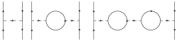
Figure 4: The first terms of perturbative series for the observed coupling constants.

We present a four-fermion interaction as a product of two color currents, taken at points $x$ and $y$ to underline its nonlocal character in the Fig. 4. As was already mentioned above, all the momentum integrations in the KKB model are factorized, and an actual integration variable is only the (virtual) quasiparticle energy. Then, the problem becomes in fact one-dimensional, that is, seems to be a simplest one in this sense. We further assume that quasiparticles with dynamical mass corresponding to the momentum transfer $p$, $M({\mbox{\boldmath$p$}})$ (in this section we will for brevity use this notation for the quark dynamical mass) take part in all virtual processes. This assumption (an approximation) seems to be quite plausible if it is taken into account that in the KKB model the quark dynamical mass, as shown, say, in Fig. 3, smoothly transforms into the mass of a bare (current) quark. It is not hard to show that a perturbative series can be expressed in terms of the polarization operator

$$\widetilde{\Pi}^{\pi,\sigma}=4N_{c}\int\frac{\textstyle d\widetilde{\mbox{\boldmath$k$}}}{\textstyle E}\frac{\textstyle-2E^{2}+M^{2}\mp M^{2}}{\textstyle(\varepsilon^{2}/4)-E^{2}}$$ (57)

(where $\varepsilon$ is the energy difference between the quarks in different spatial points, $x$ and $y$, $E=[{\mbox{\boldmath$k$}}^{2}+M^{2}({\mbox{\boldmath$k$}})]^{1/2}$ stands for the energy of a loop quasiparticle, and upper sign in the numerator corresponds to the pseudoscalar channel, and the lower sign corresponds to the scalar one), as follows:

$$G_{o}=G+VG\widetilde{\Pi}+(VG\widetilde{\Pi})^{2}+\cdots,$$ (58)

where $V$ is a volume the system is embodied in. The system volume is exactly that infrared contribution we have mentioned above. It appears to be a consequence of nonlocality of the model and assumes the form of an extra delta function $\delta^{3}(0)$. The standard regularization of the contribution coming from the latter function leads just to the factor under consideration. One can conclude from Eq. (57) that the integral contains a strong ultraviolet divergence. While discussing an expression for the quark specific energy (50), (54), we mentioned a natural way of rendering the formally divergent expressions sensible by normalizing them with respect to the free Lagrangian (Hamiltonian). Let us do the same way (in the spirit of renormalization theory) in the case at hand. To this end, we assume that the observed polarization operator $\Pi$ is given by the difference of $\widetilde{\Pi}$ and operator $\Pi_{0}$ generated by the current quarks with mass $m$,

$$\Pi=\widetilde{\Pi}-\Pi_{0}~{}.$$ (59)

Since at large momenta the quark dynamical mass smoothly transforms into the current one, it is clear that in the case of a fast enough convergence to the quark current mass, any diagram of perturbation theory will lead to a finite expression. In particular, in the chiral limit the integrals are (automatically) strictly cutoff at the momentum $2G$ ($E=(4G^{2}-{\mbox{\boldmath$p$}}^{2})^{1/2}$).

Then, represent the expression (57) as follows:

$$\widetilde{\Pi}=N_{c}~{}(\widetilde{I}+\varepsilon^{2}\widetilde{J}-\widetilde{K}^{\pi,\sigma})~{},$$ (60)

where the following notations are used

$$\widetilde{I}=2\int d\widetilde{\mbox{\boldmath$k$}}~{}\frac{\textstyle 1}{\textstyle E}~{},~{}~{}\widetilde{J}=\frac{\textstyle 1}{\textstyle 2}\int d\widetilde{\mbox{\boldmath$k$}}~{}\frac{\textstyle 1}{\textstyle E}~{}\frac{\textstyle 1}{\textstyle E^{2}-\varepsilon^{2}/4}~{},$$

$$\widetilde{K}^{\sigma}=2\int d\widetilde{\mbox{\boldmath$k$}}~{}\frac{\textstyle 1}{\textstyle E}~{}\frac{\textstyle M^{2}}{\textstyle E^{2}-\varepsilon^{2}/4}~{},~{}~{}K^{\pi}=0~{}.$$

The mass in the KKB model is related with the energy by the relation $M-m=2GM/E$. By taking into account the energy definition $E^{2}={\mbox{\boldmath$k$}}^{2}+M^{2}$, the momentum integral can be transformed in the energy one:

$$kdk=EdE~{}\left(1+\frac{\textstyle 2G~{}m^{2}}{\textstyle(E-2G)^{3}}\right)~{},$$

where

$$k=\frac{\textstyle E}{\textstyle E-2G}~{}\left[(E-2G)^{2}-m^{2})\right]^{1/2}~{}.$$

The integrals $\widetilde{I}$, $\widetilde{J}$, $\widetilde{K}$ are calculabel in terms of elementary functions. The first one is found to be

$$\widetilde{I} = \frac{\textstyle 1}{\textstyle\pi^{2}}\left[\left(\frac{\textstyle\widetilde{E}_{\Lambda}}{\textstyle 2}+2G-G\frac{\textstyle m^{2}}{\textstyle\widetilde{E}^{2}_{\Lambda}}\right)\widetilde{s}_{\Lambda}+\right.$$

$$+ \left.\frac{\textstyle 4G^{2}}{\textstyle 3}\frac{\textstyle\widetilde{s}^{3}_{\Lambda}}{\textstyle\widetilde{E}^{3}_{\Lambda}}-\frac{\textstyle m^{2}}{\textstyle 2}\ln\frac{\textstyle\widetilde{E}_{\Lambda}+\widetilde{s}_{\Lambda}}{\textstyle m}-Gm\arccos\frac{\textstyle m}{\textstyle E}~{}\right]~{},$$

where the following notation is used:

$$\widetilde{E}=E-2G~{},~{}~{}E_{\Lambda}=\left[\Lambda^{2}+M^{2}(\Lambda)\right]^{1/2}~{},$$

$$\widetilde{s}_{\Lambda}=\left[(E_{\Lambda}-2G)^{2}-m^{2}\right]^{1/2}~{},$$

$\Lambda$ is a formal upper limit of momentum integration. As we have already noted, physically meaningful results are obtained if $I_{0}$ calculated with a quark of bare mass

$$I_{0}=2\int d\widetilde{\mbox{\boldmath$k$}}~{}\frac{\textstyle 1}{\textstyle e}=\frac{\textstyle 1}{\textstyle\pi^{2}}\left(\frac{\textstyle e_{\Lambda}s_{\Lambda}}{\textstyle 2}-\frac{\textstyle m^{2}}{\textstyle 2}\ln(e_{\Lambda}+s_{\lambda})\right)~{},$$

is subtracted, where $e=(k^{2}+m^{2})^{1/2}$. By taking the cutoff integration momentum to be $\Lambda\gg G,m$ we expand the obtained expressions isolating a finite contribution

$$\lim_{\Lambda\to\infty}I=\lim_{\Lambda\to\infty}\widetilde{I}-I_{0}\to-\frac{\textstyle 1}{\textstyle\pi^{2}}~{}\left(\frac{\textstyle 10}{\textstyle 3}~{}G^{2}+\frac{\textstyle\pi}{\textstyle 2}~{}Gm\right).$$

For the integral $\widetilde{J}$ we have:

$$\widetilde{J}=\frac{\textstyle 1}{\textstyle 4\pi^{2}}\frac{\textstyle 1}{\textstyle\varepsilon}\left[j_{-}i_{-}-j_{+}i_{+}+\sum\limits_{n=1}^{4}j_{n}i_{n}\right]~{},$$ (61)

$$j_{\pm}=1-\frac{\textstyle v_{1}}{\textstyle 2G_{\pm}}+\frac{\textstyle v_{2}}{\textstyle(2G_{\pm})^{2}}-\frac{\textstyle v_{3}}{\textstyle(2G_{\pm})^{3}}+\frac{\textstyle v_{4}}{\textstyle(2G_{\pm})^{4}},$$

$$j_{1}=v_{1}a_{1}-v_{2}a_{2}+v_{3}a_{3}-v_{4}a_{4}~{},$$

$$j_{2}=v_{2}a_{1}-v_{3}a_{2}+v_{4}a_{3}~{},$$

$$j_{3}=v_{3}a_{1}-v_{4}a_{2}~{},$$

$$j_{4}=v_{4}a_{1}~{},$$

$$i_{\pm}=\int\limits_{m}^{E_{\Lambda}}dE\frac{\textstyle s}{\textstyle E_{\pm}}~{},~{}~{}i_{n}=\int\limits_{m}^{E_{\Lambda}}dE\frac{\textstyle s}{\textstyle\widetilde{E}^{n}}~{},$$

where $E_{\pm}=E\pm\varepsilon/2$, $G_{\pm}=G\pm\varepsilon/4$, $v_{1}=2G$, $v_{2}=0$, $v_{3}=2Gm^{2}$, $v_{4}=4G^{2}m^{2}$, $a_{n}=1/(2G_{-})^{n}-1/(2G_{+})^{n}$, (the terms containing $n=5$, $6$ will also appear in the expression for $K^{\sigma}$). Divergent part of the integral $J^{d}$ is given by the asymptotes of the following integrals:

$$\lim_{\Lambda\to\infty}\int\limits_{m}^{E_{\Lambda}}dE~{}\frac{\textstyle s}{\textstyle E_{\pm}}\to E_{\Lambda}-2G_{\pm}\ln\frac{\textstyle 2E_{\Lambda}}{\textstyle m}~{},$$

$$\lim_{\Lambda\to\infty}\int\limits_{m}^{E_{\Lambda}}dE~{}\frac{\textstyle s}{\textstyle\widetilde{E}}\to E_{\Lambda}~{},~{}~{}\lim_{\Lambda\to\infty}\int\limits_{m}^{E_{\Lambda}}dE~{}\frac{\textstyle s}{\textstyle\widetilde{E}^{2}}\to\ln\frac{\textstyle 2E_{\Lambda}}{\textstyle m}~{}.$$

The remaining terms in $\widetilde{J}$ are negligibly small compared with the divergent ones. Using the definition of $a_{n}$ one can see that in the asymptotic, $\Lambda\to\infty$, the integral diverges only logarithmically: $\lim_{\Lambda\to\infty}\widetilde{J}^{d}\to\frac{\textstyle 1}{\textstyle 4\pi^{2}}\ln(2E_{\Lambda}/m)$. We normalize results with respect to the free Lagrangian. Being applied to the integral $\widetilde{J}$, this means that the following contribution

$$J_{0}=\frac{\textstyle 1}{\textstyle 2}\int d\widetilde{\mbox{\boldmath$k$}}~{}\frac{\textstyle 1}{\textstyle e}~{}\frac{\textstyle 1}{\textstyle e^{2}-\varepsilon^{2}/4}~{},$$

must be subtracted. For the divergent part, it is possible to obtain $\lim_{\Lambda\to\infty}J_{0}^{d}\to\frac{\textstyle 1}{\textstyle 4\pi^{2}}\ln\frac{\textstyle 2e_{\Lambda}}{\textstyle m}$. Considering that $E_{\Lambda}\to e_{\Lambda}$, when $\Lambda\to\infty$ we see that divergent parts in $J=\widetilde{J}-J_{0}$ are exactly mutually cancelled out. For regular part one can derive:

$$J^{r} = \widetilde{J}^{r}-J^{r}_{0}~{},~{}~{}\widetilde{J}^{r}=\frac{\textstyle 1}{\textstyle 4\pi^{2}}\frac{\textstyle 1}{\textstyle\varepsilon}\biggl{[}j_{-}A_{-}-j_{+}A_{+}-$$

$$- j_{1}\left(2G+\frac{\textstyle\pi m}{\textstyle 2}\right)-j_{2}+j_{3}~{}\frac{\textstyle\pi}{\textstyle 4m}+j_{4}~{}\frac{\textstyle 1}{\textstyle 3m^{2}}\biggr{]}~{},$$

where the following notation is used:
$A_{\pm}=\!\!\left\{\begin{array}[]{l}-\left[(2G_{\pm})^{2}-m^{2}\right]^{1/2}\ln\left|\frac{\textstyle 2G_{\pm}-\left[(2G_{\pm})^{2}-m^{2}\right]^{1/2}}{\textstyle m}\right|,\\ \!\!\left[m^{2}-(2G_{\pm})^{2}\right]^{1/2}\!\!\left(\arcsin\frac{\textstyle 2G_{\pm}}{\textstyle m}-\arcsin\frac{\textstyle 2G_{\pm}+m}{\textstyle|2G_{\pm}+m|}\right).\end{array}\right.$
the upper term is valid for $|2G_{\pm}|\geq m$, the lower one, when $|2G_{\pm}|<m$. For $J^{r}_{0}$ we have:

$$J^{r}_{0}=\frac{\textstyle 1}{\textstyle 4\pi^{2}}\frac{\textstyle 1}{\textstyle\varepsilon}~{}\biggl{(}A^{0}_{-}-A^{0}_{+}\biggr{)}~{},$$

$A^{0}_{\pm}=\left\{\begin{array}[]{l}-\left[\frac{\textstyle\varepsilon^{2}}{\textstyle 4}-m^{2}\right]^{1/2}\ln\left|\frac{\textstyle\pm\frac{\textstyle\varepsilon}{\textstyle 2}-\left[\frac{\textstyle\varepsilon^{2}}{\textstyle 4}-m^{2}\right]^{1/2}}{\textstyle m}\right|,\\ \!\!\left[m^{2}-\frac{\textstyle\varepsilon^{2}}{\textstyle 4}\right]^{1/2}\!\!\left(\arcsin\frac{\textstyle\pm\varepsilon}{\textstyle 2m}-\arcsin\frac{\textstyle\pm\frac{\textstyle\varepsilon}{\textstyle 2}+m}{\textstyle\left|\pm\frac{\textstyle\varepsilon}{\textstyle 2}+m\right|}\right)~{}.\end{array}\right.$
The upper term is valid when $|\varepsilon/2|\geq m$, the lower one corresponds to the case $m>|\varepsilon/2|$. Similar results can be obtained for the integral $K^{\sigma}=\widetilde{K}^{\sigma}-K^{\sigma}_{0}$. The original integral $\widetilde{K}^{\sigma}$ can be represented in the form analogous to Eq. (61)

$$\widetilde{K}^{\sigma}=\frac{\textstyle m^{2}}{\textstyle\pi^{2}}\frac{\textstyle 1}{\textstyle\varepsilon}\left[k_{-}i_{-}-k_{+}i_{+}+\sum\limits_{n=1}^{6}k_{n}i_{n}\right]~{},$$

$$k_{\pm}=1-\frac{\textstyle w_{1}}{\textstyle 2G_{\pm}}+\cdots+\frac{\textstyle w_{6}}{\textstyle(2G_{\pm})^{6}}~{},$$

$$k_{1}=w_{1}a_{1}-\cdots-w_{6}a_{6}~{},$$

$$k_{2}=w_{2}a_{1}-\cdots+w_{6}a_{5}~{},$$

$$~{}~{}~{}~{}~{}~{}~{}~{}~{}~{}~{}~{}~{}~{}~{}~{}~{}\cdots$$

$$k_{6}=w_{6}a_{1}~{},$$

where $w_{1}=6G$, $w_{2}=12G^{2}$, $w_{3}=8G^{3}$, $w_{4}=12G^{2}m^{2}$, $w_{5}=24G^{3}m^{2}$, $w_{6}=16G^{4}m^{2}$. Isolating regular part we have

$$K_{\sigma}^{r} = \widetilde{K}_{\sigma}^{r}-K_{0\sigma}^{r}~{},$$

$$\widetilde{K}_{\sigma}^{r} = \frac{\textstyle m^{2}}{\textstyle\pi^{2}}\frac{\textstyle 1}{\textstyle\varepsilon}\biggl{[}k_{-}A_{-}-k_{+}A_{+}-k_{1}\left(2G+\frac{\textstyle\pi m}{\textstyle 2}\right)-k_{2}+$$

$$+ k_{3}~{}\frac{\textstyle\pi}{\textstyle 4m}+k_{4}~{}\frac{\textstyle 1}{\textstyle 3m^{2}}+k_{5}~{}\frac{\textstyle\pi}{\textstyle 16m^{3}}+k_{6}~{}\frac{\textstyle 2}{\textstyle 15m^{4}}\biggr{]}~{},$$

$$K_{0\sigma}^{r} = \frac{\textstyle m^{2}}{\textstyle\pi^{2}}\frac{\textstyle 1}{\textstyle\varepsilon}~{}\biggl{(}A^{0}_{-}-A^{0}_{+}\biggr{)}~{}.$$

It is convenient to use dimensionless variables $m\to m/G$, $\varepsilon\to\varepsilon/G$. One can see that the combination of the volume and coupling constant of the form $VG^{3}$ is taken for the parameter in theory, which characterizes the strength of the interaction. Generally speaking, it is also obvious from the dimensional analysis.

Figure 5: The observed coupling constant $G_{o}^{\sigma}$ as a function of the transferred energy $\varepsilon$ (in dimensionless variables). The short dash line is obtained for $m=0.9$. Dots show the case $m=0.6$. The solid line corresponds to the case $m=0.4$. Everywhere $V=1$. Point $O$ shows the location where $G_{o}^{\pi,\sigma}=0$. The long dash line corresponds to $m=0.01$.

The observed coupling constant $G_{o}$ for each individual channel separately is expressed via a regularized polarization operator:

$$G_{o}^{\pi,\sigma}=\frac{\textstyle G}{\textstyle 1-VG^{3}\Pi^{\pi,\sigma}}~{}.$$ (62)

The polarization operator $\Pi$ in this expression is presented in the dimensionless form; initially, it is proportional to the coupling constant squared: $\Pi\sim G^{2}$. So, the polarization operators introduced are free of typical logarithmical singularities and do not feature any divergent parts at all. For definiteness, consider the positive transferred energy $\varepsilon>0$ (the case of negative transferred energy is clearly symmetric). From the formulae presented it follows that the polarization operator contains strong pole singularities at the energy value $\varepsilon=4$ (in dimensional units $\varepsilon=4G$), where the variable $G_{-}$ vanishes. Local vicinity of this point, as well as actually all obtained expressions, deserves to be thoroughly studied analytically. However, in order to simplify a discussion, we will limit ourselves to carrying out a brief qualitative analysis and present for illustrative purposes a number of figures. The pole singularities (of maximal power $4$ for the integral $\widetilde{J}$ and $6$ in $\widetilde{K}$) lead to the observed coupling constant $G_{o}^{\pi,\sigma}$ vanishing at the energy value $\varepsilon=4$. It is clear that perturbation theory is valid in the vicinity of this point.

It can be shown that the bound states, defined by the denominator poles of Eq. (62) (as all the remaining contributions are negligibly small being compared with the pole singularities), may show up in this region, and a pole in the denominator may appear either right or left of the region under discussion (in dependence on the sign of high order pole singularities). Figures 5, 6 shows the energy $\varepsilon$ dependence of observed coupling constants $G_{o}^{\sigma}$, $G_{o}^{\pi}$ respectively, (in dimensionless variables). The dashed curves are obtained at $m=0.9$, while the dot curves present the case $m=0.6$, and the solid lines correspond to $m=0.4$. The system volume of the system is assumed to be a $V=1$, for definiteness. The location of point in which the observed coupling constant vanishes: $G_{o}^{\pi,\sigma}=0$ is marked as $O$. Now comparing the curves, one can clearly see the evolution of some new (’resonance’ ) state, that is manifested by a sharp and sufficiently broad peak and is transformed into a bound state, with the parameter $m$ changing from the value $m=0.9$ to $m=0.4$. (The pole singularities in both figures are somewhat smoothed in drawing in order not to lose the regular ’resonance’ structures.) In the sigma-channel several bound states simultaneously appear, when the parameter $m$ is decreasing (see a respective curve with $m=0.4$). Both figures show also the version with the parameter $m$ decreasing to the values specific for the NJL model, that is, of order $m\sim 0.01$, the corresponding data are shown by the long-dash curve. Both figures expose definitely not all the bound states. Some of those are so narrow that it is impracticable to depict them projecting on the scale used in the figures. This result makes, in principle, possible to observe a transformation of the resonance into a genuine bound state. The $m$ dependence becomes more pronounced with $VG^{3}$ parameter increasing. The observed coupling constant is substantially reduced in a low-energy region, demonstrating a transition to the qualitatively different scale. Overall, it can be concluded that if the parameter $VG^{3}$ regulating the interaction strength is small ($VG^{3}<10$), then the energy dependence of observed coupling constant is sufficiently smooth up to values $\varepsilon\sim 3$–$4$, and beyond it the bound states are coming into the play.

Figure 6: The observed coupling constant $G_{o}^{\pi}$ as a function of the energy $\varepsilon$. Notations are the same as for the scalar channel of Fig. 5.

As a consequence, an adequate picture of spontaneous breaking of chiral symmetry can be developed at this scale providing us with a reasonable information of meson observables and plausible scenario of diquark condensation.

V Conclusions

Throughout our work we have seen that picture of the ground state of fermions (quarks) ensemble developing strong correlations may significantly differ sometimes from standard scenario (accepted intuitively) of exchange interaction, obtained from our everyday experience (from condensed matter physics). The Dirac sea displays a finite relative depth, that decreases as $-\Lambda^{2}$, with momentum cutoff $\Lambda$ increasing. There exist some critical value of the coupling constant $g_{1}$ in two dimensional model and when it is weak $g<g_{1}$ the Dirac sea becomes a standard one. The Dirac sea width at $g>g_{1}$ increases linearly with momentum cutoff $\Lambda$ increasing. In the three dimension situation the width is constant. The Dirac sea width, as we show, becomes squized behaving as $\Delta_{\Lambda}\sim\frac{\textstyle D+1}{\textstyle gL^{D}D^{2}}\Lambda^{2-D}$ for spatial ($D$) dimensions. Coincidence Dirac sea width with a size of elementary cell $\widetilde{1}=2\pi/L$ (D=3) specifies a critical value of momentum cutoff as $\Lambda_{c}\approx 2N_{c}/(2gL)~{}2\pi/L$. The existing estimates teach the parameter $\Lambda_{c}$ should not develop a macroscopical value. We demonstrate the Dirac sea is strongly degenerate with respective degeneracy power proportional to the surface of ($D-1$)-dimensional sphere Clearly, such a ground state is highly unstable and according to a philosophy the Jahn–Teller theorem its energy could be lowered by reducing of its symmetry (hence removing degeneracy). It is difficult to free ourselves from an idea that similar ground state resemblance strongly the ’Big Bang’ scenario. Plausible mechanism of degeneracy removal (vacuum state reconstruction) with nonabelian (color) interaction switched on could be seen as the Bogolyubov like state of coupled quark antiquark pairs with zero total momentum and vacuum quantum numbers. The energy of such a state is getting a minimal magnitude in average. (A technical reason of this feature appearance is rooted in vanishing the contribution of tadpole diagrams.) It is interesting to notice that the models considered despite the seemingly toy form possess all the attributes of quantum field theory, including divergence. It can be seen that there are strongly singular diagrams in the intermediate perturbation theory calculations, but in final expressions there is not any trace of the divergences and, seems, the general lanscape of this theory is determined by the scenario of the Dirac sea filling.

Eventually, we would like to notice that several intuitive arguments of recent interesting development in favor of a confined quarkyonic phase existing larry receive surprisingly almost exact theoretical substantination in theframework of our consideration (of course, if deconfinement paradigm is replaced).

We are thankful to Prof. L. V. Keldysh for his insightful comments and deeply indebted to B. A. Arbuzov, S. B. Gerasimov, L. McLerran, A. M. Snigirev, L. Turko, I. P. Volobuev for fruitful discussions. The work was supported by the State Fund for Fundamental Research of Ukraine, Grant $\cal N$0 Ph58/04.

References

- (1) L. D. Faddeev, Theor. Mat. Fiz. 148 (2006) 133.
-
(2)
W. Thirring, Ann. Phys. 3 (1958) 91;
J. M. Luttinger, J. Math. Phys. 4 (1963) 1154;
D. C. Mattis and E. H. Lieb, J. Math. Phys. 6 (1965) 304. -
(3)
”Integrable Quantum Field Theories” , Lecture Notes in Physics, Vol. 151,
Springer-Verlag, New York, 1982, ed. by J. Hietarinta and C. Montonen;
N. M. Bogolyubov, A. G. Izergin, V. E. Korepin, ”Correlation function of integrable systems and quantum inverse scattering method” , Nauka, Moscow, 1992;
V. Mastropietro and D. C. Mattis, ”Luttinger model. The First 50 Years and Some New Directions” , Series on Directions in Condensed Matter Physics—Volume 20, 2014;
A. B. Zamolodchikov, Al. B. Zamolodchikov, ”Conformal Field Theory and Critical Phenomena in Two-Dimensional Systems” . -
(4)
M. V. Sadovskii, ”Diagrammatics” , Singapore: World Scientific, 2006.
L. V. Keldysh, Doctor thesis, FIAN, (1965);
E. V. Kane, Phys. Rev. 131 (1963) 79;
V. L. Bonch-Bruevich, in ”Physics of solid states” , M., VINITI, (1965). -
(5)
G. M. Zinovjev and S. V. Molodtsov, Theor. Mat. Fiz. 160 (2009) 444;
S. V. Molodtsov and G. M. Zinovjev, Phys. Rev. D 80 (2009) 076001;
S. V. Molodtsov, A. N. Sissakian and G. M. Zinovjev, Europhys. Lett. 87 (2009) 61001. - (6) B. F. Bayman, Nucl. Phys. 15 (1960) 33.
-
(7)
J. M. Blatt, Prog. Theor. Phys. 24 (1960) 851;
K. Dietrich, H. J. Mang and H. Pradal, Phys. Rev. 135 (1964) B22. - (8) Yu. A. Simonov, Phys. Lett. B 412 (1997) 371.
- (9) John von Neumann, ”Mathematical Foundation of Quantum Mechanics” , Princeton University Press, 1955.
- (10) Y. Nambu and G. Jona-Lasinio, Phys. Rev. 122 (1961) 345.
-
(11)
M. Faber and A. N. Ivanov, Eur. Phys. J. C 20 (2001) 723;
Phys. Lett. B563 (2003) 231;
T. Fujita, M. Hiramoto, T. Homma, and H. Takahashi, J. Phys. Soc. Jap. 74 (2005) 1143. - (12) T. Fujita, M. Hiramoto and H. Takahashi, ”Bosons after symmetry breaking in quantum field theory” , Nova Science Publishers, Inc. New York, 2009.
-
(13)
F. A. Berezin, ”The second quantization method” , Nauka, Moscow, 1986;
J.-P. Blaizot and G. Ripka, ”Quantum theory of Finite Systems” , The MIT Press, 1985. - (14) N. Andrei and J. H. Lowenstein, Phys. Rev. Lett. 43 (1979) 1698.
-
(15)
F. C. Alcazar, M. N. Barber, and M. T. Batchelor, Ann. Phys. 182 (1988) 280;
J. L. Cardy, J. Phys. A 17 (1984) L385;
H.W.J. Blöte, J. H. Cardy, and M. P. Nightingale, Phys. Rev. Lett. 56 (1986) 742;
I. Affleck, Phys. Rev. Lett. 56 (1986) 746. - (16) S. V. Molodtsov and G. M. Zinovjev, arXiv:1311.6606 [hep-ph].
-
(17)
S. V. Molodtsov and G. M. Zinovjev, Europhys. Lett. 93 (2011) 11001;
S. V. Molodtsov and G. M. Zinovjev, Phys. Rev. D 84 (2011) 036011;
G. M. Zinovjev and S. V. Molodtsov, Yad. Fiz. 75 (2012) 262. -
(18)
G. M. Zinovjev and S. V. Molodtsov, Yad. Fiz. 75 (2012) 1387;
G. M. Zinovjev, M. K. Volkov and S. V. Molodtsov, Theor. Mat. Fiz. 161 (2010) 408. -
(19)
V. R. Shaginyan, M. Ya. Amusia and K. G. Popov,
Usp. Fiz. Nauk. 177 (2007) 585;
S. M. Stishov, Usp. Fiz. Nauk. 174 (2004) 853;
S. Sachdev, ”Quantum phase transitions” , Cambridge University Press, 1998. -
(20)
R. W. Richardson, Phys. Lett. 3 (1963) 277;
R. W. Richardson and N. Sherman, Nucl. Phys. B52, (1964) 221;
R. W. Richardson, J. Math. Phys. 6 (1965) 1034. - (21) M. Gaudin, J. Physique 37 (1976) 1087.
- (22) M. C. Cambiaggio, A. M. F. Rivas and M. Saraceno, Nucl. Phys. A 624 (1997) 157.
-
(23)
G. Sierra, Nucl. Phys. B572 (2000) 517;
J. Dukelsky, S. Pittel and G. Sierra, Rev. Mod. Phys. 76 (2004) 643. -
(24)
L. Mclerran, R. D. Pisarski, Nucl. Phys. A796 (2007) 83;
L. Mclerran, arXiv:1105.4103 [hep-ph].