Spectral analysis of transition operators, Automata groups
and translation in BBS

Tsuyoshi Kato Department of Mathematics, Graduate School of Science, Kyoto University, Sakyo-ku, Kyoto 606–8502, Japan tkato@math.kyoto-u.ac.jp Satoshi Tsujimoto Department of Applied Mathematics and Physics, Graduate School of Informatics, Kyoto University, Sakyo-ku, Kyoto 606–8501, Japan tujimoto@i.kyoto-u.ac.jp  and  Andrzej Zuk Institut de Mathematiques, Universite Paris 7, 13 rue Albert Einstein, 75013 Paris, France andrzej.zuk@imj-prg.fr
Abstract.

We give the automata which describe time evolution rules of the box-ball system (BBS) with a carrier. It can be shown by use of tropical geometry, such systems are ultradiscrete analogues of KdV equation. We discuss their relation with the lamplighter group generated by an automaton. We present spectral analysis of the stochastic matrices induced by these automata, and verify their spectral coincidence.

Key words and phrases:
Automata groups, integrable systems, scaling limit, piece-wise linear system, PDE, tropical geometry
2000 Mathematics Subject Classification:
60G50 (primary), 20M35, 35Q53 (secondary)

1. Introduction

From the view point of dynamical systems, automata constitute semi-group actions on trees which play the essential roles in two different subjects, where one is theory of automata groups and the other is discrete integrable systems.

Both subjects have been developed from the point of view of dynamical scale transform called tropical geometry[10, 11, 18] or ultradiscretization[17] (they are essentially the same but the original sources have been different, where the former arose in real algebraic geometry and the latter from discretization of integrable systems). It provides with a correspondence between automata and real rational dynamics, which by taking scaling limits of parameters, allows us to study two dynamical systems at the same time, whose dynamical natures are very different from each other. Particularly it eliminates detailed activities in rational dynamics and extracts framework of their structure in automata, which allows us to induce some uniform analytic estimates[9].

From the computational interests, many of the integrable systems have been discretized. In particular KdV equation

(1) $\displaystyle\frac{\partial u}{\partial{t}}+6u\frac{\partial u}{\partial{x}}+\frac{\partial^{3}u}{\partial{x}^{3}}=0$

is a fundamental equation in the integrable systems, and its discretized equation has been extensively studied [3, 4], as a rational dynamical systems. In [17, 15], tropical transform has been applied to the discrete KdV equation

(2) $\displaystyle\dfrac{1}{u_{n+1}^{(t+1)}}-\dfrac{1}{u_{n}^{(t)}}=\frac{\delta}{1+\delta}\left(u_{n+1}^{(t)}-u_{n}^{(t+1)}\right),$

and the ultradiscrete KdV equation

(3) $\displaystyle B^{(t+1)}_{n}=\min(1-B^{(t)}_{n},\sum_{j=-\infty}^{n-1}(B^{(t)}_{j}-B^{(t+1)}_{j}))$

is obtained, which is the so-called box-ball systems (BBS)[13]. We verify that BBS is described by automata diagram:

[Uncaptioned image]

which is given by a direct limit of the Mealy type automata BBSk for $k\geq 1$, that are the carrier capacity extensions of BBS (see Section 3). Moreover each BBSk is described by automata diagram (Lemma 3.1).

Rational dynamics can be regarded as approximations of the corresponding evolutional systems in partial differential equations[6]. From the view point of dynamical scaling limits, automata can be regarded as frame-dynamics which play the roles of underlying mechanics for PDE[7]. From dynamical view point, distribution of orbits can be measured by probability approach, which is a quite fundamental method. So far there has been little done on study of BBS from probability aspect. On the other hand study of random walk on automata group has been extensively developed. So our basic and general question is, whether the frame dynamics of integrable systems share their structural similarity with geometric properties of automata groups. It would give us much deeper understanding of dynamical structure of BBS.

In [5], we have verified that the automaton is recursive if and only if the associated rational dynamics is quasi-recursive. Quasi-recursiveness represents ‘almost’ recursive which differs from periodic within uniform estimates independent of the choice of initial values. As an extension of the above property, we have applied tropical geometry to theory of automata groups to analyze global behaviour of real rational dynamical systems. A discrete group is called an automata group, if it is realized by actions on the rooted trees, which are represented by a Mealy automaton. The automata group is a quite important class in group theory, which have given answers to many important questions. Of particular interests for us are, counter-example to the Milnor’s conjecture, solution to the Burnside problem on the existence of finitely generated infinite torsion groups, non-uniform exponential growth groups, etc. These applications are described in [20] and [21]. As an application of tropical geometry to the construction of the Burnside group, we have verified that there exists a rational dynamical systems of Mealy type which satisfy infinite quasi-recursiveness [8]. This property again allows error from recursiveness which corresponds to infinite torsion, while rationality corresponds to finite generation.

In case of finitely generated groups one can consider as the space $l^{2}$ functions on groups and as the operator the sum of translations by chosen generators and their inverses. The study of spectra of such operators was initiated by Kesten and the normalized operators are called random walk or transition operators [19].

In general it is a very difficult problem to compute spectra of these operators. Some important progresses have been achieved by studying different approximations of such operators using the representations of the group, in particular their actions on finite sets. For instance in [1] the spectrum of the random walk operator on the Heisenberg group was computed using approximations Harper operators via theory of rotational algebras. In case of groups generated by automata one can study their actions on finite sequences. The simplest case when one obtains an interesting spectral information is the automaton on two states which generated the lamplighter group. All other two state automata lead to very elementary cases. In the case of BBS we do not deal with invertible transformations which would define groups. However we can still define the operators similar to random walk operators and consider their action on finite sequences. This enables us to compute the limit spectral measures for such sequences as was done for automata in [2].

Even though both BBS and automata group are constructed from Mealy automata, their scopes are quite different. As a result, one finds quite different characteristics from each other. It would be of particular interest for us to combine such properties via dynamical study of Mealy automata. We want to investigate BBS systems via spectra of some operators associated to them, as it is common in non-commutative geometry.

Recall that both the lamplighter group and BBS act on the rooted binary tree $T$. For convenience let us describe its action in the case of the lamplighter group (see Section 2.1). Each state acts on the binary tree, and in this case there are two actions ${\bf A}_{q_{0}}$ and ${\bf A}_{q_{1}}$ corresponding to the state set $\{q_{0},q_{1}\}$. It is defined inductively on each level set. The actions on the second level set are depicted as follows:

[Uncaptioned image]

In general transition operators of automata can be given by filtration of finite rank matrices with respect to the restriction of the action on each level set. It was known that these matrices of the lamplighter automaton all satisfy stochastic property. Such property is quite important for automata groups in relation to random walk on automata groups. In comparison to BBS automata, we have verified that the same property holds for all $k\geq 1$.

Let $\{M_{k}^{(n)}\}_{n\geq 1}$ be the filtration of the transition operators for BBSk. They are defined in Section 3.1 by $\frac{1}{2k+2}\sum_{i=0}^{k}(a_{i}^{\!(n)}+a_{i}^{\!(n)*})$, where $a_{i}^{(n)}$ are the restrictions of the representation matrices on the level $n$ set and the superscript $*$ denotes the transpose of the matrix.

Proposition (Proposition 4.1).

The matrix $M_{k}^{(n)}$ is double stochastic for all $k\geq 1$, $n\geq 0$, i.e. the sum of each row and each column is equal to $1$.

It is known that there is an example of Mealy automata whose transition operators do not satisfy stochastic property.

The simplest case BBS $k=1$ (BBS translation) satisfies rather trivial behavior from dynamics view points, since it is translation. However the above proposition would suggest that BBS translation is closely related to the cases for $k\geq 2$. Concerning BBS translation, we have discovered non trivial phenomena from spectral analysis view point.

Theorem (Theorem 4.2).

(i) The spectra of the transition operators coincide with each other between the lamplighter group as an automata group and the BBS translation. It is totally discrete and dense in $[-1,1]$.

Because the eigenvalue distributions coincide, we may expect that both transition operators are mutually conjugate by some orthogonal matrices. Actually we verify that it certainly holds. Moreover it would be natural to ask whether the conjugation might be chosen from tree automorphisms.

We have the negative answer:

Proposition (Proposition 5.5).

There are no automorphisms of $T$ which conjugate between $M_{L}^{(n)}$ and $M_{B}^{(n)}$.

On the other hand, one might still ask whether it comes from permutations, or from an automorphism of the one sided shift. We have the affirmative answer, which gives the complete answer to the conjugations.

Let $M_{B}^{(n)},M_{L}^{(n)}\in\mbox{Mat}(2^{n}\times 2^{n};{\mathbb{R}})$. Let us denote the set of indices as $I_{n}=\{0,1,\ldots,2^{n}-1\}$.

Theorem (Theorem 6.1).

There exists a permutation matrix $\sigma_{n}$, such that

$\displaystyle\sigma_{n}^{*}M_{B}^{(n)}\sigma_{n}=M_{L}^{(n)}$

holds. We have the explicit recurrence formulas for $\sigma_{n}$ which involves the Sierpinski gasket pattern.

In the cases for $k\geq 2$, we present numerical computations of the spectral distributions and observe that there exist structural similarities in the distributions of eigenvalues between the BBSk and the lamplighter group. Based on the observations, we give conjectures (Conjecture 4.4 and 4.5).

If one reduces an integrable system to an automaton by extracting its dynamical framework, then it should posses high symmetry, which will have some structural similarity with finitely generated groups. It would be interesting to investigate further coincidence between spectra of automata associated to integrable system and the one associated to automata groups.

2. Automata groups

An automaton is defined by finite rules which can create quite complicated state dynamics over the sequences of alphabets.

Let $Q$ and $S$ be finite sets, and consider the set of all infinite sequences:

$$S^{\mathbb{N}}=\{(s_{0},s_{1},\dots):s_{i}\in S\}.$$

A Mealy automaton ${\bf A}$ is given by a pair of functions:

$$\varphi:Q\times S\to Q,\quad\psi:Q\times S\to S$$

which gives rise to the state dynamics on $S^{\mathbb{N}}$ as follows. Let us choose any $q\in Q$ and $\bar{s}=(s_{0},s_{1},\dots)\in S^{\mathbb{N}}$. Then:

$${\bf A}_{q}:S^{\mathbb{N}}\to S^{\mathbb{N}}$$

${\bf A}_{q}(\bar{s})=(s_{0}^{\prime},s_{1}^{\prime},\dots)$ is determined inductively by:

$$s_{i}^{\prime}=\psi(q_{i},s_{i}),\quad q_{i+1}=\varphi(q_{i},s_{i})\quad(q_{0}=q).$$

Besides the dynamics over $S^{\mathbb{N}}$, the change of the state sets play important roles in a hidden dynamics.

Any sequences $\bar{q}^{j}=(q^{0},\dots,q^{j})\in Q^{j+1}$ give dynamics by compositions:

$${\bf A}_{\bar{q}^{j}}={\bf A}_{q^{j}}\circ\dots\circ{\bf A}_{q^{0}}:S^{\mathbb{N}}\to S^{\mathbb{N}}.$$

It can happen that different automata give the same state dynamics. In such a case, the dynamics of ${\bf A}_{q}$ are the same, but the systems of change of state sets can be very different. Such two automata are called equivalent.

Suppose

$$\psi:(q,\quad):S\to S$$

are permutations for all $q\in Q$. If we identify $S^{\mathbb{N}}$ with the rooted tree, then the Mealy dynamics give the group actions on the tree, since the actions can be restricted level-setwisely. The group generated by these states is called the automata group given by the automaton $(\varphi,\psi)$.

Next we introduce the diagram expression of the automaton ${\bf A}$ defined via the quadruple $(Q,S,\varphi,\psi)$. In the diagram each vertex corresponds to a state $q\in Q$. When $\varphi(q,i)=r$ and $\psi(q,i)=j$, the vertex $q$ is connected to the vertex $r$ with the directional arrow equipped with the pair of input and output strings, $i\mid j$.

2.1. Lamplighter group

The lamplighter group:

$$(\oplus_{\mathbb{Z}}{\mathbb{Z}}_{2})\rtimes{\mathbb{Z}}$$

is generated by canonical generators, which are $v$, one copy of ${\mathbb{Z}}_{2}$, and $u$, the generator of ${\mathbb{Z}}$.

The corresponding automaton can be represented by the following diagram:

[Uncaptioned image]

which shows that the quadruple $(Q,S,\varphi,\psi)$ of the lamplighter group as an automata group is given by

$\displaystyle Q=\{q_{0},q_{1}\},\quad S=\{0,1\},$
$\displaystyle\varphi(q_{0},0)=0,\quad\varphi(q_{0},1)=1,\quad\varphi(q_{1},0)=0,\quad\varphi(q_{1},1)=1,$
$\displaystyle\psi(q_{0},0)=1,\quad\psi(q_{0},1)=0,\quad\psi(q_{1},0)=0,\quad\psi(q_{1},1)=1.$

For example, we give actions of the lamplighter automata ${\bf A}_{q_{0}}$ and ${\bf A}_{q_{1}}$ as follows:

$\displaystyle{\bf A}_{q_{0}}(0011101100000\cdots)=1101100101111\cdots$
$\displaystyle{\bf A}_{q_{1}}(0011101100000\cdots)=0101100101111\cdots$

Let $a_{i}$ be the infinite matrix representations of ${\bf A}_{q_{i}}$ for $i=0,1$. They decompose into $2$ by $2$ matrices with operator valued entries, with respect to

$$S^{\mathbb{N}}=S^{\mathbb{N}}_{0}\sqcup S^{\mathbb{N}}_{1}$$

where $S^{\mathbb{N}}_{i}=\{(i,s_{1},\dots):s_{i}\in S\}$.

In the lamplighter case, we have two operator recursions [2]

(8) $\displaystyle a_{0}=\left(\begin{array}[]{cc}0&a_{1}\\ a_{0}&0\\ \end{array}\right),\quad a_{1}=\left(\begin{array}[]{cc}a_{0}&0\\ 0&a_{1}\\ \end{array}\right),$

where $a_{1}^{-1}a_{0}$ corresponds to $v$ and $a_{0}$ to $u$.

3. BBS with carrier capacity

The BBS is one of the ultradiscrete integrable systems. The BBS is composed of an array of infinitely many boxes, finite number of balls in the boxes, and a carrier of balls. Each box can contain only one ball and the carrier can hold arbitrary number of balls. The evolution rule from time $j$ to time $j+1$ is defined as follows. The carrier moves from left to right and passes each box. When the carrier passes a box containing a ball, the carrier gets the ball; when the carrier passes an empty box, if the carrier holds balls, the carrier puts one ball into the box.


Figure 1. A two-soliton interaction of the BBS

Let us describe BBS with carrier capacity $k$ [12]. In this case the carrier can hold at most $k$ balls. The only difference with the previous situation is that when the carrier holds $k$ balls and passes a box containing a ball, the carrier does nothing.

Similar to the case of KdV, the BBS with carrier capacity $k$ can be obtained from the discrete modified KdV equation [14]

(9) $\displaystyle v_{n+1}^{(t+1)}\dfrac{(1+\alpha)v_{n}^{(t+1)}+\delta}{(1+\delta)v_{n}^{(t+1)}+\alpha}=v_{n}^{(t)}\dfrac{(1+\alpha)v_{n+1}^{(t)}+\delta}{(1+\delta)v_{n+1}^{(t)}+\alpha},$

where $\alpha,\delta$ are constants, which reduces to the modified KdV equation

$\displaystyle\frac{\partial{v}}{\partial t}+6\beta{v}^{2}\frac{\partial{v}}{\partial x}+\dfrac{1}{4\beta}\frac{\partial^{3}{v}}{\partial{x}^{3}}=0,$

where $\beta$ is a constant. The BBS with carrier capacity $k$ is presented by

$\displaystyle\widetilde{B}_{n}^{(t+1)}=\min\left(1-\widetilde{B}_{n}^{(t)},\sum_{j=-\infty}^{n-1}(\widetilde{B}_{j}^{(t)}-\widetilde{B}_{j}^{(t+1)})\right)+\max\left(0,\sum_{j=-\infty}^{n}(\widetilde{B}_{j}^{(t)}-\widetilde{B}_{j-1}^{(t+1)})-k\right).$
Lemma 3.1.

The diagram expression of the BBS with carrier capacity $k$ is given by

[Uncaptioned image]

The (simple) BBS is obtained as the limiting case of the above automaton with $k\to\infty$.

Proof.

The state $q_{i}$ corresponds to the situation when the carrier holds $i$ balls. Thus we start at the state $q_{0}$. If we have 1 as the input we go from the state $q_{i}$ to $q_{i+1}$ if $i<k$ and we change 1 to 0. This corresponds to the fact the carrier picks up the ball if the number of balls it already holds is $i<k$. If we have 0 as the input we go from the state $q_{i}$ to $q_{i-1}$ if $i>0$ and change 1 to 0. This corresponds to the fact the carrier puts the ball if the number of balls it already holds is at least 1. It remains to check the situation for $q_{0}$ with the input 0 and for $q_{k}$ with the input 1. The first one corresponds to the carrier with 0 balls passing an empty box (it does nothing and still holds no balls) and the last one to the carrier with $k$ balls passing a box with a ball (it does nothing and still holds $k$ balls). ∎

3.1. BBS translation (carrier capacity $k=1$)

The BBS translation can be represented by

[Uncaptioned image]

For example, we give actions of the BBS translation ${\bf A}_{q_{0}}$ and ${\bf A}_{q_{1}}$ as follows:

$\displaystyle{\bf A}_{q_{0}}(0011101100000\cdots)=0001110110000\cdots$
$\displaystyle{\bf A}_{q_{1}}(0011101100000\cdots)=1001110110000\cdots$

Let $a_{i}$ be the infinite matrix representations of ${\bf A}_{q_{i}}$ for $i=0,1$. Then we have two operator recursions

(14) $\displaystyle a_{0}=\left(\begin{array}[]{cc}a_{0}&a_{1}\\ 0&0\\ \end{array}\right),\quad a_{1}=\left(\begin{array}[]{cc}0&0\\ a_{0}&a_{1}\\ \end{array}\right).$

We can describe the action of $a_{0}$ and $a_{1}$ on the binary sequences of length $n$ by the $2^{n}\times 2^{n}$ matrices $a_{0}^{(n)}$ and $a_{1}^{(n)}$. From the definition of our automaton, they satisfy the following recurrence relations:

$\displaystyle a_{0}^{(0)}=a_{1}^{(0)}=1,$
$\displaystyle a^{(n+1)}_{0}=\left(\begin{array}[]{cc}a^{(n)}_{0}&a^{(n)}_{1}\\[2.84526pt] 0&0\\ \end{array}\right),\quad a^{(n+1)}_{1}=\left(\begin{array}[]{cc}0&0\\ a^{(n)}_{0}&a^{(n)}_{1}\\ \end{array}\right).$

In the case when ${\bf A}_{q_{j}}$ for $j=0,1$ give automorphisms so that they constitute an automata group, the transition operator is given by $M=\frac{1}{4}(a_{0}+a_{0}^{*}+a_{1}+a_{1}^{*})$ which describes step $1$ random walk. In the general case when the actions are not invertible, one can still consider the same operators, since the adjoint operators coincide with the inverse ones for the invertible case, since they are unitaries. The actions by ${\bf A}_{q_{j}}$ are always deterministic, while its adjoint ${\bf A}_{q_{j}}$ are non-deterministic in non invertible case. A key observation is that random walk on semi-groups is still possible to formulate and would be quite natural, if we allow non deterministic actions and interpret them as probability processes. In this paper we shall introduce the transition operator over the semi-groups by the same formula.

Let us consider the filtrations of the transition operators:

$\displaystyle M_{k=1}^{(n)}=\dfrac{1}{4}\left(a^{(n)}_{0}+a^{(n)*}_{0}+a^{(n)}_{1}+a^{(n)*}_{1}\right).$

3.2. BBS with carrier capacity $k=2$

In analogy to $k=1$ case, for $k=2$, we can consider the following operators.

[Uncaptioned image]

For example, we give actions of the BBSk=2 ${\bf A}_{q_{0}},{\bf A}_{q_{1}}$ and ${\bf A}_{q_{2}}$ as follows:

$\displaystyle{\bf A}_{q_{0}}(0011101100000\cdots)=0000110111000\cdots$
$\displaystyle{\bf A}_{q_{1}}(0011101100000\cdots)=1000110111000\cdots$
$\displaystyle{\bf A}_{q_{2}}(0011101100000\cdots)=1100110111000\cdots$

Notice that the state $q_{j}$ corresponds to the carrier with $j$-number of balls. The action ${\bf A}_{q_{j}}$ represents the time-evolution of BBSk dynamics with carrier with $j$-number of balls as an initial state.

Let $a_{i}$ be the infinite matrix representations of ${\bf A}_{q_{i}}$ for $i=0,1,2$. Then we have three operator recursions

$\displaystyle a_{0}=\left(\begin{array}[]{cc}a_{0}&a_{1}\\ 0&0\\ \end{array}\right),\quad a_{1}=\left(\begin{array}[]{cc}0&a_{2}\\ a_{0}&0\\ \end{array}\right),\quad a_{2}=\left(\begin{array}[]{cc}0&0\\ a_{1}&a_{2}\\ \end{array}\right).$

The action of $a_{0},a_{1}$ and $a_{2}$ on the binary sequences of length $n$ can be described by the $2^{n}\times 2^{n}$ matrices $a_{0}^{(n)},a_{1}^{(n)}$ and $a_{2}^{(n)}$ which satisfy the following recurrence relations:

$\displaystyle a_{0}^{(0)}=a_{1}^{(0)}=a_{2}^{(0)}=1,$
$\displaystyle a^{(n+1)}_{0}=\left(\begin{array}[]{cc}a^{(n)}_{0}&a^{(n)}_{1}\\[2.84526pt] 0&0\\ \end{array}\right),\quad a^{(n+1)}_{1}=\left(\begin{array}[]{cc}0&a^{(n)}_{2}\\ a^{(n)}_{0}&0\\ \end{array}\right),\quad a^{(n+1)}_{2}=\left(\begin{array}[]{cc}0&0\\ a^{(n)}_{1}&a^{(n)}_{2}\\ \end{array}\right).$

The filtrations of the transition operators are given by

$\displaystyle M^{(n)}_{k=2}=\dfrac{1}{6}\left(a^{(n)}_{0}+a^{(n)*}_{0}+a^{(n)}_{1}+a^{(n)*}_{1}+a^{(n)}_{2}+a^{(n)*}_{2}\right).$

In the next sections, we will verify that these transition operators are stochastic and analyze in detail the spectral properties of the transition operator for $k=1$ theoretically and $k\geq 2$ numerically.

4. Stochastic matrices

Study of countably state ergodic Markov chain is an important subject in relation with statistic mechanics. However because of countably many number of the states, construction of the probability measures on the path space has not been so developed. It follows from Corollary 5.4 below that BBS transition operators $M^{(n)}_{k}$ give the ergodic Markov chains over the set of paths $\Omega(n)$ which are given by $\Omega(n)=\{(w_{1},w_{2},\dots)\mid w_{i}\in\{1,\dots,2^{n}\}\}$ with the unique ergodic distributions $\pi^{(n)}=(\pi_{1}^{(n)},\dots,\pi^{(n)}_{2^{n}})$ [16]. Let $m_{k}$ be the probability measure on $\Omega(n)$. One may expect that the family of ergodic Markov chains defined by $\{M_{k}^{(n)}\}_{n=1}^{\infty}$ can give a countably state Markov chains over the path space:

$$\Omega(\infty)=\{(w_{1},w_{2},\dots)\mid w_{i}\in{\mathbb{N}}\ \}$$

which is expected ergodic at the limit.

Let us verify stochastic property of the transition operators for BBSk. We define a sequence of $k+1$ matrices $(a_{0}^{(n)},\ldots,a_{k}^{(n)})$ of dimension $2^{n}$, for $n=0,1,\ldots$ by the following matrix recursion (00 represents here $2^{n}\times 2^{n}$ null matrix).

$$a_{0}^{(n+1)}=\left(\begin{array}[]{cc}a_{0}^{(n)}&a_{1}^{(n)}\\ 0&0\end{array}\right)$$

For $i=1,\ldots,k-1$

$$a_{i}^{(n+1)}=\left(\begin{array}[]{cc}0&a_{i+1}^{(n)}\\ a_{i-1}^{(n)}&0\end{array}\right)$$

and

$$a_{k}^{(n+1)}=\left(\begin{array}[]{cc}0&0\\ a_{k-1}^{(n)}&a_{k}^{(n)}\end{array}\right)$$

with the initial data $a_{i}^{(0)}=1$ for all $i=0,\ldots,k$.

We consider the following $2^{n}\times 2^{n}$ matrix $M_{k}^{(n)}$

$$M_{k}^{(n)}=\frac{1}{2k+2}(a_{0}^{(n)}+a_{0}^{(n)*}+\ldots+a_{k}^{(n)}+a_{k}^{(n)*}).$$
Proposition 4.1.

The matrix $M_{k}^{(n)}$ is double stochastic for all $k\geq 1$, $n\geq 0$, i.e. the sum of each row and each column is equal to $1$.

Proof.

The matrix $M_{k}^{(n)}$ is symmetric and therefore it suffices to prove that the sum of columns is constant.

Clearly the recursive relations for $a_{0}^{{(n+1)}},\ldots,a_{k}^{{(n+1)}}$ show that the matrix we obtain from each of them is the matrix with constant sum of columns (equal to $k$).

Thus it is enough to show that $a_{0}^{(n)*}+\ldots+a_{k}^{(n)*}$ has constant column sum. Let us prove this by induction. It is clear for $n=0$. Then using recursion formula

$$a_{0}^{(n+1)*}+\cdots+a_{k}^{(n+1)*}=\left(\begin{array}[]{cc}a_{0}^{(n)*}&a_{k-1}^{(n)*}+\cdots+a_{0}^{(n)*}\\ a_{1}^{(n)*}+\cdots+a_{k}^{(n)*}&a_{k}^{(n)*}\end{array}\right)$$

and thus the sum of the left matrix blocks and right matrix blocks is equal to

$$a_{0}^{(n)*}+\ldots+a_{k}^{(n)*}.$$

Therefore the statement follows by induction. ∎

4.1. Spectral computation for BBS translation ($k=1$)

Stochastic property closely related to random walk on each level set of the binary tree. On the other hand structure of the random walk heavily depends on their spectral distribution. First we compute the spectral distribution of the transition operator for $k=1$:

$\displaystyle M_{k=1}^{(n)}=\dfrac{1}{4}\left(a^{(n)}_{0}+a^{(n)*}_{0}+a^{(n)}_{1}+a^{(n)*}_{1}\right).$

Define the counting spectral measures of $M^{(n)}_{k}$, i.e. $\sigma_{k}^{(n)}:[0,1]\to[0,1]$ and for $x\in[0,1]$ by:

$$\sigma_{k}^{(n)}(x)=\dfrac{\sharp\left\{\lambda\in\mbox{Sp}(M_{k}^{(n)})\mid\lambda\leq 2(k+1)\cos(\pi x)\right\}}{\sharp\left\{\lambda\in\mbox{Sp}(M_{k}^{(n)})\right\}}.$$

Let us denote the multiplicity of eigenvalue $\lambda$ of $M^{(n)}_{k}$ by

$\displaystyle m^{(n;k)}(\lambda)=\sharp\{\lambda\in\mbox{Sp}(M_{k}^{(n)})\}.$

In particular we denote the multiplicity of eigenvalue $\cos\left(pq^{-1}\pi\right)$ of $M^{(n)}_{k}$ by $m_{p,q}^{(n;k)}=m^{(n;k)}\left(\cos\left(pq^{-1}\pi\right)\right)$.

We consider the case $k=1$ and provide the computation of eigenvalues of $M_{k=1}^{(n)}$. Our computation on the spectra verify the following:

Theorem 4.2.
$\displaystyle\mbox{Sp}\left(M_{k=1}^{(n)}\right)=\mbox{Sp}\left(\dfrac{1}{4}\sum_{j=0}^{1}\left(a^{(n)}_{j}+a^{(n)*}_{j}\right)\right)=\left\{1\cup\cos\left(\dfrac{p}{q}\pi\right)\bigg{|}\,p,q\in{\mathbb{N}},1\leq p<q\leq n+1\right\}$

If $p$ and $q$ are mutually prime, then the multiplicity of eigenvalue $\cos\left(pq^{-1}\pi\right)$, denoted by $m_{p,q}^{(n;1)}$, is given by

$\displaystyle m_{p,q}^{(n;1)}=\left[2^{n}\left(\dfrac{2^{-q}-2^{-q\left(\left[\frac{n}{q}\right]+1\right)}}{1-2^{-q}}\right)\right]$

In order to simplify the notation we define $a_{n}=a_{0}^{(n)}$ and $b_{n}=a_{1}^{(n)}$.

Lemma 4.3.

For every $n$

$$a_{n}a_{n}^{*}+b_{n}b_{n}^{*}=2\text{Id}_{\,2^{n}}.$$
Proof.

We have

$$a_{n+1}a_{n+1}^{*}=\left(\begin{array}[]{cc}a_{n}&b_{n}\\ 0&0\end{array}\right)\left(\begin{array}[]{cc}a_{n}^{*}&0\\ b_{n}^{*}&0\end{array}\right)=\left(\begin{array}[]{cc}a_{n}a_{n}^{*}+b_{n}b_{n}^{*}&0\\ 0&0\end{array}\right)$$
$$b_{n+1}b_{n+1}^{*}=\left(\begin{array}[]{cc}0&0\\ a_{n}&b_{n}\end{array}\right)\left(\begin{array}[]{cc}0&a_{n}^{*}\\ 0&b_{n}^{*}\end{array}\right)=\left(\begin{array}[]{cc}0&0\\ 0&a_{n}a_{n}^{*}+b_{n}b_{n}^{*}\end{array}\right)$$

and the statement follows by induction. ∎

Proof of Theorem $6.1$: Let us put:

$$\Phi_{n}(\lambda,\mu)=\det(a_{n}+a_{n}^{*}+b_{n}+b_{n}^{*}-\frac{1}{2}\mu(a_{n}b_{n}^{*}+b_{n}a_{n}^{*})-\lambda Id_{2^{n}})$$

Then by use of Lemma 4.3, we have the equalities:

$\displaystyle\Phi_{n+1}(\lambda,\mu)$ $\displaystyle=\det(a_{n+1}+a_{n+1}^{*}+b_{n+1}+b_{n+1}^{*}-\frac{1}{2}\mu(a_{n+1}b_{n+1}^{*}+b_{n+1}a_{n+1}^{*})-\lambda Id_{2^{n+1}})$
$\displaystyle=\det\left(\begin{array}[]{cc}a_{n}+a_{n}^{*}-\lambda&b_{n}+a_{n}^{*}-\frac{1}{2}\mu(a_{n}a_{n}^{*}+b_{n}b_{n}^{*})\\ a_{n}+b_{n}^{*}-\frac{1}{2}\mu(a_{n}a_{n}^{*}+b_{n}b_{n}^{*})&b_{n}+b_{n}^{*}-\lambda\end{array}\right)$
$\displaystyle=\det\left(\begin{array}[]{cc}a_{n}+a_{n}^{*}-\lambda&b_{n}+a_{n}^{*}-\mu\\ a_{n}+b_{n}^{*}-\mu&b_{n}+b_{n}^{*}-\lambda\end{array}\right)$
$\displaystyle=\det\left(\begin{array}[]{cc}a_{n}-b_{n}-\lambda+\mu&b_{n}+a_{n}^{*}-\mu\\ a_{n}-b_{n}+\lambda-\mu&b_{n}+b_{n}^{*}-\lambda\end{array}\right)$
$\displaystyle=\det\left(\begin{array}[]{cc}2\mu-2\lambda&a_{n}^{*}-b_{n}^{*}-\mu+\lambda\\ a_{n}-b_{n}+\lambda-\mu&b_{n}+b_{n}^{*}-\lambda\end{array}\right)$

Using the fact that

$$\det\left(\begin{array}[]{cc}A&B\\ C&D\end{array}\right)=\det(AD-CB)$$

provided that $A$ commutes with $C$ we get

$\displaystyle\Phi_{n+1}(\lambda,\mu)$ $\displaystyle=\det((2\mu-2\lambda)(b_{n}+b_{n}^{*}-\lambda)-(a_{n}-b_{n}+\lambda-\mu)(a_{n}^{*}-b_{n}^{*}-\mu+\lambda))$
$\displaystyle=\det((\mu-\lambda)(a_{n}+a_{n}^{*}+b_{n}+b_{n}^{*})-\frac{1}{2}2(a_{n}b_{n}^{*}+b_{n}a_{n}^{*})+(-2+\lambda^{2}-\mu^{2})Id_{2^{n}})$

Therefore

$$\Phi_{n+1}(\lambda,\mu)=(\mu-\lambda)^{2^{n}}\Phi_{n}\left(\frac{2-\lambda^{2}+\mu^{2}}{\mu-\lambda},\frac{-2}{\mu-\lambda}\right).$$

This is exactly the formula from [2] which leads to the explicit computation of all eigenvalues.

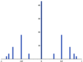
4.2. Numerical computation of spectra for BBS ($k\geq 2$)

In order to analyze spectral characteristics of the transition operators for k2𝑘2k\geq 2, as a first step, we did numerical computation of the spectral distributions for k=2,3,4,5𝑘2345k=2,3,4,5. 
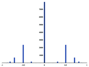
Let us compare the histogram of the spectral distributions for k=1𝑘1k=1 and 222. Figures 222 and 333 present the histogram of the distributions of the multiple eigenvalues for k=1𝑘1k=1, n=7𝑛7n=7, and k=2𝑘2k=2, n=14𝑛14n=14 respectively. Roughly we can see their structural similarity.

Refer to caption
Figure 2. Distribution of the multiple eigenvalues of $M_{k=1}^{(7)}$
Refer to caption
Figure 3. Distribution of the multiple eigenvalues of $M_{k=2}^{(14)}$

Let us see more detailed distributions for k=1,2,,5𝑘125k=1,2,\ldots,5 by Tables 1, …, 4 below. The tables present the distribution of the non-negative eigenvalues with multiplicities larger than or equal to 222. We have listed only non-negative eigenvalues, where negative ones appear symmetrically for k=1𝑘1k=1. For k=2,3,4,5𝑘2345k=2,3,4,5 cases also, negative eigenvalues appear almost symmetrically on their multiplicities, except a few values. Actually their monotonicity with respect to n𝑛n hold. 
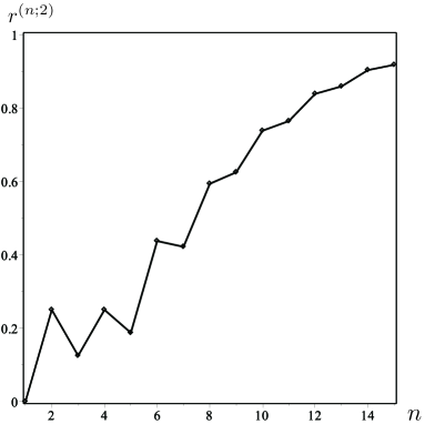
We also present the growth of the rates of r(n;k)superscript𝑟𝑛𝑘r^{(n;k)} for k=2𝑘2k=2 in Figure 4.

Observe the following structural similarity of $k=2,3,4,5$ cases to $k=1$:

  1. (1)

    The eigenvalues for $k\geq 2$, which are monotone increasing with respect to large $n$ coincide with the ones for $k=1$.

  2. (2)

    One can find structural similarity of the distributions of the eigenvalues. Another multiple eigenvalues appear on every $k$ steps for large $n$ as is the case for $k=1$. The order of appearance of the another multiple eigenvalues coincide. More concretely, for $k=1$, another eigenvalue $\cos\frac{p}{n-1}\pi$ appear at the $n$-stage as multiple eigenvalues, and then they grow monotonically. For $k=2$, there corresponds to $\cos\frac{2p}{n}\pi$ with $n=2,4,6,\dots$. For general $k$, the eigenvalues are of the form $\cos\frac{p\pi}{\lfloor\frac{n-2}{k}\rfloor+1}$, where $\lfloor\ \rfloor$ is the largest integer not greater than itself (Gauss symbol).

  3. (3)

    Below in the tables 4 and 5, some of the eigenvalues are the extra ones which do not appear for $k=1$ case. They are included in the sets $\frac{\pm 1}{k+1},\frac{\pm 2}{k+1},\dots$.

  4. (4)

    The rates of the multiple eigenvalues $r^{(n;k)}=2^{-n}\{\ \sum_{i,j}m^{(n;k)}_{i,j}+\sum_{j}m^{(n;k)}(\frac{\pm j}{k+1})\ \}$ in Figure 4 seems to grow to $1$ with respect to $n$.

Based on these observations, we would like to propose the followings:

Conjecture 4.4.

Let $j$ be a non-negative integer and let $\hat{\text{Sp}}(M_{k=j}^{(n)})\subset\text{Sp}(M_{k=j}^{(n)})$ be the set of multiple eigenvalues. Then:

$$\text{Sp}(M_{k=1}^{\left(\lfloor(n-2)/j\rfloor\right)})=\{1\}\cup\left(\hat{\text{Sp}}(M_{k=j}^{(n)})\cap\hat{\text{Sp}}(M_{k=j}^{(n+1)})\right)\quad\mbox{for}\quad n\geq 3.$$
Conjecture 4.5.

Let $j$ be a non-negative integer. There are $n_{\lambda,j}\in{\mathbb{N}}$ so that the following equalities hold:

$\displaystyle\lim_{n\to\infty}\mbox{Sp}\left(M_{k=1}^{(n)}\right)=\lim_{n\to\infty}\left\{\lambda\in\mbox{Sp}\left(M_{k=j}^{(n)}\right)\,\big{|}\,0<m^{(n_{\lambda,j};j)}(\lambda)\leq\cdots\leq m^{(n-1;j)}(\lambda)\leq m^{(n;j)}(\lambda)\right\}.$
Table 1. Multiplicities of non-negative eigenvalues for $k=1$
$n$ $m_{1,2}^{(n;1)}$ $m_{1,3}^{(n;1)}$ $m_{1,4}^{(n;1)}$ $m_{1,5}^{(n;1)}$ $m_{2,5}^{(n;1)}$ $m_{1,6}^{(n;1)}$ $m_{1,7}^{(n;1)}$ $m_{2,7}^{(n;1)}$ $m_{3,7}^{(n;1)}$ $m_{1,8}^{(n;1)}$ $\cdots$ $m_{5,11}^{(n;1)}$
1 1 0 0 0 0 0 0 0 0 0 0
2 1 1 0 0 0 0 0 0 0 0 0
3 3 1 1 0 0 0 0 0 0 0 0
4 5 2 1 1 1 0 0 0 0 0 0
5 11 5 2 1 1 1 0 0 0 0 0
6 21 9 4 2 2 1 1 1 1 0 0
7 43 18 9 4 4 2 1 1 1 1 0
8 85 37 17 8 8 4 2 2 2 1 0
9 171 73 34 17 17 8 4 4 4 2 0
10 341 146 68 33 33 16 8 8 8 4 1
Table 2. Multiplicities of non-negative multiple eigenvalues for $k=2$
$n$ $m_{1,2}^{(n;2)}$ $m_{1,3}^{(n;2)}$ $m_{1,4}^{(n;2)}$ $m_{1,5}^{(n;2)}$ $m_{2,5}^{(n;2)}$ $m_{1,6}^{(n;2)}$ $m_{1,7}^{(n;2)}$ $m_{2,7}^{(n;2)}$ $m_{3,7}^{(n;2)}$
1 0 0 0 0 0 0 0 0 0
2 1 0 0 0 0 0 0 0 0
3 0 0 0 0 0 0 0 0 0
4 4 0 0 0 0 0 0 0 0
5 6 0 0 0 0 0 0 0 0
6 22 3 0 0 0 0 0 0 0
7 42 6 0 0 0 0 0 0 0
8 104 21 3 0 0 0 0 0 0
9 210 50 6 0 0 0 0 0 0
10 460 118 24 3 3 0 0 0 0
11 930 252 54 6 6 0 0 0 0
12 1940 551 144 25 25 3 0 0 0
13 3906 1134 306 60 60 6 0 0 0
14 7966 2359 692 165 165 28 3 3 3
15 16002 4788 1434 366 366 66 6 6 6
Table 3. Multiplicities of non-negative multiple eigenvalues for $k=3$
$n$ $m^{(n;3)}(\frac{1}{4})$ $m_{1,2}^{(n;3)}$ $m_{1,3}^{(n;3)}$ $m_{1,4}^{(n;3)}$ $m_{1,5}^{(n;3)}$ $m_{2,5}^{(n;3)}$
1 0 0 0 0 0 0
2 0 0 1 0 0 0
3 0 1 0 0 0 0
4 2 0 0 0 0 0
5 0 4 0 0 0 0
6 0 7 0 0 0 0
7 0 26 0 0 0 0
8 0 56 2 0 0 0
9 0 151 7 0 0 0
10 0 332 26 0 0 0
11 0 776 68 2 0 0
12 0 1653 196 7 0 0
13 0 3640 464 30 0 0
14 0 7604 1152 80 2 2
15 0 16157 2570 256 7 7
Table 4. Multiplicities of non-negative multiple eigenvalues for $k=4$ and $5$
$k=4$
$n$ $m^{(n;4)}(\frac{1}{5})$ $m_{1,2}^{(n;4)}$ $m_{1,3}^{(n;4)}$ $m_{1,4}^{(n;4)}$
1 0 0 0 0
2 0 0 0 0
3 0 0 1 0
4 0 1 0 0
5 2 0 0 0
6 0 3 0 0
7 1 6 0 0
8 0 29 0 0
9 3 62 0 0
10 0 185 2 0
11 5 418 6 0
12 0 1061 31 0
13 9 2332 80 0
14 0 5427 265 2
15 15 11704 652 6
$k=5$
$n$ $m^{(n;5)}(\frac{1}{6})$ $m^{(n;5)}(\frac{2}{6})$ $m_{1,2}^{(n;5)}$ $m_{1,3}^{(n;5)}$
1 0 0 0 0
2 0 0 0 0
3 0 0 0 0
4 0 0 0 1
5 0 1 1 0
6 1 0 0 0
7 0 1 4 0
8 0 0 6 0
9 0 3 33 0
10 0 0 69 0
11 0 5 220 0
12 0 0 500 2
13 0 9 1333 6
14 2 0 3002 34
15 0 15 7327 93
Refer to caption
Figure 4. Rates of the multiple eigenvalues $r^{(n;k)}$ for $k=2$

So far we have found some similarity of spectral distributions for various $k\geq 1$. It is quite unexpected for us to find any kind of structural similarity among BBSk and the lamplighter automaton, since BBSk=1 is dynamically translation invariant, while BBSk≥2 behave essentially nonlinear. It would be reasonable to expect to see more concrete dynamical similarity for several $k\geq 1$. On the other hand extra appearance of new eigenvalues are observed for $k\geq 2$, which might lead to see essential difference of dynamics among BBSk (see $(3)$ above). Combination with these opposite phenomena will lead us with much deeper understanding of BBS.

5. Ergodicity of the transition operators for BBS translation

5.1. Ergodicity on the boundary of the binary tree

Let $\{M_{1}^{(n)}\}_{n=1,2,\dots}$ be the family of transition operators for lamplighter or BBSk=1 automata. We have verified that those are stochastic $2^{n}$ by $2^{n}$ matrices equipped with the canonical maps:

$$\dots\to M_{1}^{(n+1)}\to M_{1}^{(n)}\to\dots$$
Definition 5.1.

Let $M$ be a stochastic $k$ by $k$ matrix. $M$ is ergodic, if there is $s_{0}\geq 1$ and $\alpha>0$ so that inequalities:

$$m_{i,j}^{(s_{0})}\geq\alpha$$

hold for all $i,j$, where $M^{s}=(m_{i,j}^{(s)})_{1\leq i,j\leq k}$.

For stochastic matrix, if the above property is satisfied for some $s_{0}$, then the same property holds for all $s\geq s_{0}$.

Recall the fundamental result on ergodicity:

Theorem 5.1.

Let $M$ be a stochastic $k$ by $k$ matrix, and consider the associated transition chain on the space $X=\{1,\dots,k\}$. If $M$ is ergodic, then there is a unique probability distribution $\pi$ on $X$ which satisfies two properties (1) $\pi M=\pi$, and (2) $\lim_{s\to\infty}m_{i,j}^{(s)}=\pi_{j}$.

The unique probability distribution $\pi=(\pi_{1},\dots,\pi_{k})$ is called the stationary distribution with respect to $M$.

Lemma 5.2.

$M$ is ergodic, if and only if the spectrum of $M$ satisfies

(1) the multiplicity of the eigenvalue $1$ is just $1$, and

(2) it does not contain $-1$.

Proof.

Suppose $M$ is ergodic. Let $v_{1}$ and $v_{2}$ be two orthogonal eigenvectors with eigenvalue $1$. Then $v_{i}M=v_{i}$ hold, and so:

$$\langle v_{1}M^{2s},v_{2}\rangle=\langle v_{1}M^{s},v_{2}M^{s}\rangle=\langle v_{1},v_{2}\rangle=0$$

must hold. Let $a_{i}$ be the sum of coordinates of $v_{i}$. Then $a_{i}$ can not be zero, since $v_{i}=\lim_{s\to\infty}v_{i}M^{s}=a_{i}\pi$ hold by Theorem 5.1. By letting $s\to\infty$ in the above equalities, it follows $\pi=0$ is zero vector, which is a contradiction, since $\pi_{i}\geq\alpha>0$. So the multiplicity of the eigenvalue $1$ must be less than or equal to $1$. It is at least $1$ because constant vectors have eigenvalue $1$.

As we noticed that the limit exists:

$$wM^{s}\equiv(x_{1},\dots,x_{n})M^{s}\to(a\pi_{1},\dots,a\pi_{n})$$

by Theorem 5.1, where $a=\sum_{i=1}^{n}x_{i}$. But if $w$ is an eigenvector with eigenvalue $-1$, then $wM^{s}\in\{w,-w\}$ oscillates, which is a contradiction.

Suppose the above two properties hold. Let $\{v_{1},\dots,v_{k}\}$ be the orthogonal eigenvectors such that $v_{1}$ corresponds to the eigenvalue $1$. Then for any $v=\sum_{i=1}^{k}a_{i}v_{i}$,

$$\lim_{s\to\infty}vM^{s}=a_{1}v_{1}+\lim_{s\to\infty}\sum_{i=2}^{k}\lambda_{i}^{s}a_{i}v_{i}=a_{1}v_{1}$$

hold, since $-1<\lambda_{i}<1$ hold for $i\geq 2$.

Suppose $M$ is not ergodic, i.e. for every $s$, there exist $i,j$ such that $m_{i,j}^{(s)}=0$ hold. Let $\delta_{i}=(0,\dots,0,1,0,\dots)$. Then $\langle\delta_{i}M^{s},\delta_{j}\rangle=m_{i,j}^{(s)}=0$ holds. It follows that there exist $i,j$ such that $\langle\delta_{i}M^{l},\delta_{j}\rangle=0$ hold for infinitely many $l$. So it also holds for $l\to\infty$. It follows that $\delta_{i}$ or $\delta_{j}$ is orthogonal to $v_{1}$. Since $M$ is stochastic, we can put $v_{1}=(1,\dots,1)$, and so this is a contradiction. This completes the proof. ∎

Remark 5.3.

For the stochastic matrix, the property (1) is equivalent to connectivity, and property (2) is to non bi-partiteness of the associated graph.

Corollary 5.4.

Let $M_{L}^{(n)}$ and $M_{B}^{(n)}$ be the transition operators for the lamplighter and BBSk=1 automata, respectively. Then they are all ergodic.

Proof.

The result follows from our computation of their spectra in Theorem $7.1$ with Lemma 5.2. ∎

5.2. On automorphisms of the tree

Let $T$ be the binary tree, and $T_{n}$ be $n$-th level set. Then the transition operators satisfy:

$$M^{(n+1)}|_{T_{n}}=M^{(n)}.$$

Let us consider the canonical maps:

$$\dots\to M^{(n+1)}\to M^{(n)}\to\dots$$

and take the projective limit:

$$M\equiv\lim_{\leftarrow n}M^{(n)}.$$

$M$ gives an ergodic transition chain on $\partial T$, if $M^{(n)}$ are ergodic.

Proposition 5.5.

There are no automorphisms of $T$ which conjugate between $M_{L}^{(n)}$ and $M_{B}^{(n)}$.

Proof.

If there were an automorphism of the tree which would conjugate two operators on some level $n$ it would also conjugate these operators on the previous levels. Thus it is enough to prove the statement for the level $n=2$. For this level the operator corresponding to the BBS system has $(2,0,0,2)$ on the diagonal and the operator corresponding to the lamplighter has $(0,0,2,2)$ on the diagonal. The last one under the tree automorphism can be transformed to itself or $(2,2,0,0)$ only. ∎

6. Conjugacy by permutation for BBS translation

Let $M_{B}^{(n)},M_{L}^{(n)}\in\mbox{Mat}(2^{n}\times 2^{n};\mathbb{Z})$. Let us denote the set of indices as $I_{n}=\{0,1,\ldots,2^{n}-1\}$. We denote the concatenation of two vectors $u\in\mathbb{C}^{n}$ and $v\in\mathbb{C}^{m}$ by $(u,v)\in\mathbb{C}^{n+m}$. For $c\in I_{n}$, consider the binary expansion :

$$c=\sum_{j=1}^{n}c_{j}\,2^{n-j}\in I_{n}$$

where $c_{j}\in{\mathbb{Z}}_{2}$, which we denote as:

$$c=(c_{1},c_{2}\cdots,c_{n})_{2}.$$

In this section, we verify the following:

Theorem 6.1.

There exists a family of the transformation matrices $\sigma_{n}$ such that

$\displaystyle\sigma_{n}^{*}M_{B}^{(n)}\sigma_{n}=M_{L}^{(n)}$

hold, where $\sigma_{n}$ is determined by the permutation vector $\displaystyle\widehat{\sigma}_{n}=\left(\mu_{0}^{(n)},\mu_{1}^{(n)},\cdots,\mu_{2^{n}-1}^{(n)}\right)$ by

$\displaystyle\sigma_{n}e_{j}=e_{\mu_{j}^{(n)}}$

for any $j\in I_{n}$, where $e_{j}=(0,\dots,0,1,0,\dots,0)^{*}$.

The permutation vectors $\widehat{\sigma}_{n}=(\mu_{0}^{(n)},\mu_{1}^{(n)},\ldots,\mu_{2^{n}-1}^{(n)})$ are uniquely determined by

  • $\widehat{\sigma}_{1}=(\mu_{0}^{(1)},\mu_{1}^{(1)})=(0,1)$,

  • there exists a binary sequence $\nu^{(n)}=(\nu^{(n)}_{0},\nu^{(n)}_{1},\ldots,\nu^{(n)}_{2^{n-1}-1})\in\{0,1\}^{2^{n-1}}$ such that

    (18) $\displaystyle\widehat{\sigma}_{n}=(\widehat{\sigma}_{n-1},\widehat{\sigma}_{n-1})+2^{n-1}(1-\nu_{0}^{(n)},\nu_{0}^{(n)},\ldots,1-\nu_{2^{n-1}-1}^{(n)},\nu_{2^{n-1}-1}^{(n)}),$
  • the binary sequences $\nu^{(n)}\in\{0,1\}^{2^{n}-1}$ are determined by use of the binary pattern $g$ of the Sierpinski gasket as follows:

    (19) $\displaystyle\nu^{(n)}=(T_{g^{(n)}_{1}}\circ T_{g^{(n)}_{2}}\circ\cdots\circ T_{g^{(n)}_{n-1}})(0)$

    for $n\geq 2$. The operator $T_{\alpha}$ is defined by

    $\displaystyle T_{\alpha}(s_{1},s_{2},\ldots,s_{m})=\left\{\begin{array}[]{ll}(s_{1},s_{2},\ldots,s_{m},s_{1},s_{2},\ldots,s_{m})&\mbox{if $\alpha=0$}\\ (s_{1},s_{2},\ldots,s_{m},1-s_{1},1-s_{2},\ldots,1-s_{m})&\mbox{if $\alpha=1$}\\ \end{array}\right..$

    Here the binary pattern $g$ of the Sierpinski gasket is given by $g_{1}^{(n)}=g_{n}^{(n)}=1$ and

    $$g^{(n)}_{m}=g^{(n-1)}_{m-1}+g^{(n-1)}_{m}\mod 2\,\,$$

    for $m=2,3,\ldots,n-1$ and $n=1,2,\ldots$ .

Remark 6.2.

(1) Let us see the orbit of $g$:

$\displaystyle g^{(1)}=(g^{(1)}_{1})=(1),$
$\displaystyle g^{(2)}=(g^{(2)}_{1},g^{(2)}_{2})=(1,1),$
$\displaystyle g^{(3)}=(g^{(3)}_{1},g^{(3)}_{2},g^{(3)}_{3})=(1,0,1),$
$\displaystyle g^{(4)}=(g^{(4)}_{1},g^{(4)}_{2},g^{(4)}_{3},g^{(4)}_{4})=(1,1,1,1),$
$\displaystyle g^{(5)}=(g^{(5)}_{1},g^{(5)}_{2},g^{(5)}_{3},g^{(5)}_{4},g^{(5)}_{5})=(1,0,0,0,1),$
$\displaystyle g^{(6)}=(g^{(6)}_{1},g^{(6)}_{2},g^{(6)}_{3},g^{(6)}_{4},g^{(6)}_{5},g^{(6)}_{6})=(1,1,0,0,1,1),$
$\displaystyle g^{(7)}=(g^{(7)}_{1},g^{(7)}_{2},g^{(7)}_{3},g^{(7)}_{4},g^{(7)}_{5},g^{(7)}_{6},g^{(7)}_{7})=(1,0,1,0,1,0,1),\ldots.$

which gives the pattern of the Sierpinski gasket.

(2) Another formula of $g$ is given by:

$$g_{m}^{(n)}=\frac{(n-1)!}{(m-1)!(n-m)!}\mod 2$$
Corollary 6.3.

The formulas hold for all $k\in I_{n-1}$:

$$\mu_{2k}^{(n)}+\mu_{2k+1}^{(n)}=2^{n}-1,\quad\mu_{2k}^{(n)}\in 2I_{n-1}.$$
Proof.

We proceed by induction. Suppose the conclusion holds up to $n-1$. It follows from (18) that

$\displaystyle\mu_{2k}^{(n)}+\mu_{2k+1}^{(n)}$ $\displaystyle=\mu_{2k}^{(n-1)}+\mu_{2k+1}^{(n-1)}+2^{n-1}$
$\displaystyle=2^{n}-1.$

The latter formula follows immediately. ∎

Let us denote $[n]\in\mathbb{Z}_{2}$ by the image of $n$ by $\mathbb{Z}\to\mathbb{Z}_{2}$.

Lemma 6.4.

(i) $\nu^{(n)}$ is given by

$\displaystyle\nu^{(n)}_{k}=\nu^{(n)}_{(k_{1},k_{2},\cdots,k_{n-1})_{2}}=\bigg{[}\sum_{j=1}^{n-1}k_{j}g_{j}^{(n)}\bigg{]}.$

(ii) $\widehat{\sigma}_{n}=(\mu_{0}^{(n)},\mu_{1}^{(n)},\ldots,\mu_{2^{n}-1}^{(n)})$ is a permutation vector of $I_{n}$, that is,

$$\mu_{j}^{(n)}\in I_{n},\quad\mu_{j}^{(n)}\neq\mu_{j^{\prime}}^{(n)}\text{ for all distinct pairs }j\neq j^{\prime}$$
Proof.

(i) Let us rewrite $T_{\alpha}$ as:

$$T_{\alpha}(s_{1},s_{2},\ldots,s_{m})=([s_{1}],[s_{2}],\ldots,[s_{m}],[s_{1}+\alpha],[s_{2}+\alpha],\ldots,[s_{m}+\alpha]).$$

For example we see the case of $\nu^{(4)}$,

$\displaystyle\nu^{(4)}=$ $\displaystyle(T_{g_{1}^{(4)}}\circ T_{g_{2}^{(4)}}\circ T_{g_{3}^{(4)}})(0)$
$\displaystyle=$ $\displaystyle(0,[g_{3}^{(4)}],[g_{2}^{(4)}],[g_{2}^{(4)}+g_{3}^{(4)}],[g_{1}^{(4)}],[g_{1}^{(4)}+g_{3}^{(4)}],[g_{1}^{(4)}+g_{2}^{(4)}],[g_{1}^{(4)}+g_{2}^{(4)}+g_{3}^{(4)}]),$

and

$\displaystyle\nu^{(4)}_{(0,0,0)_{2}}=[0+0+0],\ \nu^{(4)}_{(0,0,1)_{2}}=[0+0+g_{3}^{(4)}],\ \nu^{(4)}_{(0,1,0)_{2}}=[0+g_{2}^{(4)}+0],$
$\displaystyle\nu^{(4)}_{(0,1,1)_{2}}=[0+g_{2}^{(4)}+g_{3}^{(4)}],$
$\displaystyle\nu^{(4)}_{(1,0,0)_{2}}=[g_{1}^{(4)}+0+0],\nu^{(4)}_{(1,0,1)_{2}}=[g_{1}^{(4)}+0+g_{3}^{(4)}],\ldots.$

Let us consider the general case. For any $h_{j}\in\{0,1\}$, let us define

$\displaystyle v=(v_{0},\cdots,v_{2^{n-1}-1})=(T_{h_{n-1}}\circ T_{h_{n-2}}\circ\cdots\circ T_{h_{1}})(0)$
$\displaystyle\tilde{v}=(\tilde{v}_{0},\cdots,\tilde{v}_{2^{n}-1})=(T_{h_{n}}\circ T_{h_{n-1}}\circ T_{h_{n-2}}\circ\cdots\circ T_{h_{1}})(0)$
$\displaystyle\quad=(v,v+h_{n})\mod 2.$

If $v_{k}=v_{(k_{1},\cdots,k_{n-1})_{2}}=[\sum_{j=1}^{n-1}k_{j}h_{n-j}]$, then

$$\tilde{v}_{\tilde{k}}=\tilde{v}_{(\tilde{k}_{1},\ldots,\tilde{k}_{n})_{2}}=[v_{k}+\tilde{k}_{1}h_{n}]=\bigg{[}\sum_{j=1}^{n}\tilde{k}_{j}h_{n-j+1}\bigg{]}$$

for $\tilde{k}\in\{0,\cdots,2^{n}-1\}$, since $k_{1}=\tilde{k}_{2},\cdots,k_{n-1}=\tilde{k}_{n}$ hold.

If we insert $g_{i}^{(n)}$ into $h_{n-i}$ in $v$, then we obtain $\nu^{(n)}$, that is

$$\nu^{(n)}_{k}=\bigg{[}\sum_{j=1}^{n-1}k_{j}g_{j}^{(n)}\bigg{]}.$$

(ii) We proceed by induction. For $n=1$, $\widehat{\sigma}_{1}=(0,1)$ corresponds to the identity over $I_{1}=\{0,1\}$.

Suppose that the conclusion holds up to $n-1$ so that $\widehat{\sigma}_{n-1}$ be a permutation vector of $I_{n-1}$. It follows from the expression (i) that for any $k_{2},\ldots,k_{n-1}\in\{0,1\}$, the equalities hold:

$\displaystyle[\nu^{(n)}_{(0,k_{2},\cdots,k_{n-1})_{2}}+\nu^{(n)}_{(1,k_{2},\cdots,k_{n-1})_{2}}]=\bigg{[}g_{1}^{(n)}+2\sum_{j=2}^{n-1}k_{j}g_{j}^{(n)}\bigg{]}=g_{1}^{(n)}=1.$

In particular $\nu^{(n)}_{(0,k_{2},\cdots,k_{n-1})_{2}}\neq\nu^{(n)}_{(1,k_{2},\cdots,k_{n-1})_{2}}$, and hence

$\displaystyle|\mu_{j}^{(n)}-\mu_{j+2^{n-1}}^{(n)}|=g_{1}^{(n)}2^{n-1}=2^{n-1}$

hold for any $j\in I_{n-1}$.

By the assumption, $\widehat{\sigma}_{n-1}$ is a permutation vector on $I_{n-1}$ so that $\mu_{j}^{(n)}\neq\mu_{l}^{(n)}$ hold for any distinct pair $0\leq j,l\leq 2^{n-1}-1$. Since the value of $\mu_{j}^{(n)}$ does not exceed $2^{n}$, it follows that $\mu_{j}^{(n)}\neq\mu_{l}^{(n)}$ hold for any distinct pair $0\leq j,l\leq 2^{n}-1$, and hence $\widehat{\sigma}_{n}$ must be a permutation vector of $I_{n}$. ∎

Proposition 6.5.

$\widehat{\sigma}_{n}^{2}=$ id hold on $I_{n}=\{0,1,\dots,2^{n}-1\}$.

Proof.

Let $k\in I_{n}$. For $k=(k_{1},k_{2},\ldots,k_{n})_{2}$, let us denote the corresponding binary expansions:

$\displaystyle\widehat{\sigma}_{n}(k)$ $\displaystyle=\widehat{\sigma}_{n}((k_{1},k_{2},\ldots,k_{n})_{2})=(k_{1}^{\prime},k_{2}^{\prime},\ldots,k_{n}^{\prime})_{2},$
$\displaystyle\widehat{\sigma}_{n}^{2}(k)$ $\displaystyle=\widehat{\sigma}_{n}((k_{1}^{\prime},k_{2}^{\prime},\ldots,k_{n}^{\prime})_{2})=(k_{1}^{\prime\prime},k_{2}^{\prime\prime},\ldots,k_{n}^{\prime\prime})_{2},$

respectively. Firstly let us verify the formulas:

(21) $\displaystyle\widehat{\sigma}_{n}(k)$ $\displaystyle=\left(\widehat{\nu}_{(k_{1},k_{2},\ldots,k_{n-1})_{2}}^{(n;k_{n})},\widehat{\nu}_{(k_{2},\ldots,k_{n-1})_{2}}^{(n-1;k_{n})},\ldots,\widehat{\nu}_{(k_{n-1})_{2}}^{(2;k_{n})},k_{n}\right)_{2}$

where $\widehat{\nu}^{(n-\kappa+1;k_{n})}_{(k_{\kappa},\ldots,k_{n-1})_{2}}\in\{0,1\}$ is defined by

$\displaystyle\widehat{\nu}_{(k_{\kappa},\ldots,k_{n-1})_{2}}^{(n-{\kappa}+1;k_{n})}\equiv[1+\nu_{(k_{\kappa},\ldots,k_{n-1})_{2}}^{(n-{\kappa}+1)}+k_{n}]=\bigg{[}1+\sum_{i=1}^{n-{\kappa}+1}k_{{\kappa}+i-1}g_{i}^{(n-{\kappa}+1)}\bigg{]}.$

Since $\hat{\sigma}_{1}=(0,1)$, one can see that $\widehat{\sigma}_{1}(0)=0$ and $\widehat{\sigma}_{1}(1)=1$.

Notice that $\nu^{(2)}=T_{g_{1}^{(2)}}(0)=T_{1}(0)=(0,1)$ and hence

$\displaystyle\hat{\sigma}_{2}$ $\displaystyle=(\hat{\sigma}_{1},\hat{\sigma}_{1})+2(1-\nu_{0}^{(2)},\nu_{0}^{(2)},1-\nu_{1}^{(2)},\nu_{1}^{(2)})$
$\displaystyle=(0,1,0,1)+2(1-0,0,1-1,1)=(2,1,0,3).$

It can be presented as

$\displaystyle(\widehat{\nu}_{k_{1}}^{(2;k_{2})},k_{2})_{2}=(1+k_{1}g_{1}^{(2)}+k_{2},k_{2})_{2}=2[1+k_{1}+k_{2}]+k_{2},$

for any $k\in I_{2}$. In fact the equalities follow from direct computations:

$\displaystyle\widehat{\sigma}_{2}(0)=2[1+0+0]+0=2,\quad\widehat{\sigma}_{2}(1)=2[1+0+1]+1=1,$
$\displaystyle\widehat{\sigma}_{2}(2)=2[1+1+0]+0=0,\quad\widehat{\sigma}_{2}(3)=2[1+1+1]+1=3.$

Suppose the formula holds up to $n-1$. Then we have the equalities:

(22) $\displaystyle\widehat{\sigma}_{n}(k)$ $\displaystyle=\widehat{\sigma}_{n}((k_{1},k_{2},\ldots,k_{n})_{2})$
(25) $\displaystyle=\widehat{\sigma}_{n-1}((k_{2},k_{3},\ldots,k_{n})_{2})+\left\{\begin{array}[]{lr}2^{n-1}\nu_{(k_{1},k_{2},\ldots,k_{n-1})_{2}}^{(n)}&\text{ if $k_{n}=1$}\\ 2^{n-1}(1-\nu_{(k_{1},k_{2},\ldots,k_{n-1})_{2}}^{(n)})&\text{ if $k_{n}=0$}\end{array}\right.$
$\displaystyle=(0,\widehat{\nu}_{(k_{2},k_{3},\ldots,k_{n-1})_{2}}^{(n-1;k_{n})},\cdots,\widehat{\nu}_{(k_{n-1})_{2}}^{(2;k_{n})},k_{n})_{2}+(1+\nu_{(k_{1},k_{2},\ldots,k_{n-1})_{2}}^{(n)}+k_{n},0,\ldots,0)_{2}$
$\displaystyle=\left(\widehat{\nu}_{(k_{1},k_{2},\ldots,k_{n-1})_{2}}^{(n;k_{n})},\widehat{\nu}_{(k_{2},\ldots,k_{n-1})_{2}}^{(n-1;k_{n})},\ldots,\widehat{\nu}_{(k_{n-1})_{2}}^{(2;k_{n})},k_{n}\right)_{2}.$

So it holds for $n$.

Next by use of (21), we obtain the equalities:

(26) $\displaystyle k_{\kappa}^{\prime}$ $\displaystyle=\bigg{[}1+\sum_{i=1}^{n-{\kappa}+1}k_{{\kappa}+i-1}g_{i}^{(n-{\kappa}+1)}\bigg{]},\quad k_{n}^{\prime}=k_{n},$
(27) $\displaystyle k_{\kappa}^{\prime\prime}$ $\displaystyle=\bigg{[}1+\sum_{i=1}^{n-{\kappa}+1}k_{{\kappa}+i-1}^{\prime}g_{i}^{(n-{\kappa}+1)}\bigg{]},\quad k_{n}^{\prime\prime}=k_{n},$

where $\kappa=1,2,\ldots,n-1$. For $n-\kappa\in\{1,2,\ldots,n-1\}$,

$\displaystyle k_{n-\kappa}^{\prime\prime}$ $\displaystyle=\bigg{[}1+\sum_{j=1}^{\kappa+1}k_{n-\kappa+j-1}^{\prime}g_{j}^{(\kappa+1)}\bigg{]}$
$\displaystyle=\bigg{[}1+\sum_{j=1}^{\kappa}(1+\sum_{l=1}^{\kappa-j+2}k_{n-\kappa+j+l-2}g_{l}^{(\kappa-j+2)})g_{j}^{(\kappa+1)}+k_{n}^{\prime}g_{\kappa+1}^{(\kappa+1)}\bigg{]}$
$\displaystyle=\bigg{[}1+\sum_{j=1}^{\kappa}(1+\sum_{l=1}^{\kappa-j+2}k_{n-\kappa+j+l-2}g_{l}^{(\kappa-j+2)})g_{j}^{(\kappa+1)}+k_{n}g_{1}^{(1)}g_{\kappa+1}^{(\kappa+1)}]$
$\displaystyle=\bigg{[}1+\sum_{j=1}^{\kappa}\left(g_{j}^{(\kappa+1)}\right)+k_{n-\kappa}g_{1}^{(\kappa+1)}g_{1}^{(\kappa+1)}$
$\displaystyle\qquad+(\sum_{j=1}^{\kappa}\sum_{l=1}^{\kappa-j+2}k_{n-\kappa+j+l-2}g_{l}^{(\kappa-j+2)}g_{j}^{(\kappa+1)})-k_{n-\kappa}g_{1}^{(\kappa+1)}g_{1}^{(\kappa+1)}+k_{n}g_{1}^{(1)}g_{\kappa+1}^{(\kappa+1)}\bigg{]}$
$\displaystyle=\bigg{[}1+\sum_{j=1}^{\kappa}\left(g_{j}^{(\kappa+1)}\right)+k_{n-\kappa}g_{1}^{(\kappa+1)}g_{1}^{(\kappa+1)}+\sum_{j=2}^{\kappa+1}k_{n-\kappa+j-1}\left(\sum_{l=1}^{j}g_{j-l+1}^{(\kappa-l+2)}g_{l}^{(\kappa+1)}\right)\bigg{]}$
$\displaystyle=k_{n-\kappa},$

where we have used the equalities $g_{1}^{(1)}=g_{1}^{(\kappa+1)}=g_{\kappa+1}^{(\kappa+1)}=1,[1+\sum_{j=1}^{\kappa}\left(g_{j}^{(\kappa+1)}\right)]=0$,

$\displaystyle g_{j-l+1}^{(\kappa-l+2)}g_{l}^{(\kappa+1)}$ $\displaystyle=\bigg{[}\dfrac{\kappa!}{(\kappa-j+1)!(j-l)!(l-1)!}\bigg{]}=g_{j-(j-l+1)+1}^{(\kappa-(j-l+1)+2)}g_{j-l+1}^{(\kappa+1)},$
$\displaystyle g_{m+1}^{(\kappa-m+1)}g_{m+1}^{(\kappa+1)}$ $\displaystyle=g_{2m+1-(m+1)+1}^{(\kappa-(m+1)+2)}g_{m+1}^{(\kappa+1)}=\bigg{[}\dfrac{\kappa!}{(\kappa-2m)!\,m!\,m!}\bigg{]}$
$\displaystyle=\bigg{[}\dfrac{(2m)!}{m!\,m!}\dfrac{\kappa!}{(\kappa-2m)!\,(2m)!}\bigg{]}=\bigg{[}2\binom{2m-1}{m}{\kappa\choose 2m}\bigg{]}=0,$

and

$\displaystyle\bigg{[}\sum_{l=1}^{j}g_{j-l+1}^{(\kappa-l+2)}g_{l}^{(\kappa+1)}\bigg{]}$ $\displaystyle=\begin{cases}\bigg{[}2\sum_{l=1}^{m}g_{j-l+1}^{(\kappa-l+2)}g_{l}^{(\kappa+1)}\bigg{]}&(j=2m)\\[7.11317pt] \bigg{[}2\sum_{l=1}^{m}g_{j-l+1}^{(\kappa-l+2)}g_{l}^{(\kappa+1)}+g_{m+1}^{(\kappa-m+1)}g_{m+1}^{(\kappa+1)}\bigg{]}&(j=2m+1)\\ \end{cases}$
$\displaystyle=0.$

Hence $\widehat{\sigma}_{n}^{2}(k)=(k_{1},k_{2},\ldots,k_{n})_{2}=k$ holds. ∎

Proof of Theorem 6.1.

Let $j,k\in I_{n}$, and denote the binary expansions:

$\displaystyle j=(j_{1},j_{2},\ldots,j_{n})_{2},\quad k=(k_{1},k_{2},\ldots,k_{n})_{2},$
$\displaystyle\widehat{\sigma}_{n}(j)=(j_{1}^{\prime},j_{2}^{\prime},\ldots,j_{n}^{\prime})_{2},\quad\widehat{\sigma}_{n}(k)=(k_{1}^{\prime},k_{2}^{\prime},\ldots,k_{n}^{\prime})_{2}.$

Let us denote the two generating elements $a_{0},a_{1}$ of the dynamics for the lamplighter operators (8) and the BBS (14) by:

$$a_{L}^{(0)},\ a_{L}^{(1)},\ a_{B}^{(0)},\ a_{B}^{(1)}$$

respectively. These operators satisfy the following recursive relations for $\varepsilon=0,1$:

$$a_{L}^{(\varepsilon)}=([j+k+\varepsilon]a_{L}^{(k)})_{0\leq j,k\leq 1},\quad a_{B}^{(\varepsilon)}=([j+1+\varepsilon]a_{B}^{(k)})_{0\leq j,k\leq 1}.$$

By applying these formulas repeatedly, we obtain four matrices of the size $2^{n}$ by $2^{n}$ given by

$\displaystyle a_{B}^{(\varepsilon;n)}=\bigg{(}\alpha^{(\varepsilon)}_{j,k}\bigg{)}_{0\leq j,k<2^{n}}=\bigg{(}[(j_{1}+1+\varepsilon)(j_{2}+1+k_{1})\cdots(j_{n}+1+k_{n-1})]\bigg{)}_{0\leq j,k\leq 2^{n}-1},$
$\displaystyle a_{L}^{(\varepsilon;n)}=\bigg{(}\beta^{(\varepsilon)}_{j,k}\bigg{)}_{0\leq j,k<2^{n}}=\bigg{(}[(j_{1}+k_{1}+\varepsilon)(j_{2}+k_{2}+k_{1})\cdots(j_{n}+k_{n}+k_{n-1})]\bigg{)}_{0\leq j,k\leq 2^{n}-1}.$

We shall verify the stronger formulas:

(28) $\displaystyle a_{B}^{(0;n)}+a_{B}^{(1;n)}=\sigma_{n}\left(a_{L}^{(0;n)}+a_{L}^{(1;n)}\right)\sigma_{n}^{-1}.$

This is enough to conclude proposition:

$\displaystyle M_{B}^{(n)}$ $\displaystyle=a_{B}^{(0;n)}+a_{B}^{(1;n)}+a_{B}^{(0;n)*}+a_{B}^{(1;n)*}$
$\displaystyle=\sigma_{n}\left(a_{L}^{(0;n)}+a_{L}^{(1;n)}+a_{L}^{(0;n)*}+a_{L}^{(1;n)*}\right)\sigma_{n}^{-1}=\sigma_{n}M_{L}^{(n)}\sigma_{n}^{-1}.$

Since $\widehat{\sigma}_{n}$ is a permutation vector (Proposition 6.4) and $\widehat{\sigma}_{n}^{-1}=\widehat{\sigma}_{n}$ (Proposition 6.5), equation (28) is equivalent to the equalities:

(29) $\displaystyle\alpha^{(0)}_{j,k}+\alpha^{(1)}_{j,k}=\beta^{(0)}_{\widehat{\sigma}_{n}(j),\widehat{\sigma}_{n}(k)}+\beta^{(1)}_{\widehat{\sigma}_{n}(j),\widehat{\sigma}_{n}(k)}$

for all $j,k\in I_{n}$.

Let us compute both sides, and divide into two cases on $(j_{2}+1+k_{1})(j_{3}+1+k_{2})\cdots(j_{n}+1+k_{n-1})$, where:

  • (i)

    all the factors $j_{i+1}+1+k_{i}\,(i=1,2,\ldots,n-1)$ take odd integer values,

  • (ii)

    otherwise, that is, there exists an integer $\kappa$ such that $j_{\kappa+1}+1+k_{\kappa}$ is even.

To treat both cases, we claim the following formula: suppose for some $1\leq\kappa\leq n$,

$$j_{i+1}+k_{i}+1$$

is odd for $\kappa+1\leq i\leq n-1$, then

(30) $\displaystyle[j_{i}^{\prime}+k_{i}^{\prime}+k_{i-1}^{\prime}]=[j_{i}+k_{i-1}+1]$

for $\kappa+1\leq i\leq n$.

In fact we have the equalities:

$\displaystyle[j_{i}^{\prime}+k_{i}^{\prime}+k_{i-1}^{\prime}]$ $\displaystyle=\bigg{[}3+\sum_{l=1}^{n-i+1}(j_{i+l-1}+k_{i+l-1})g_{l}^{(n-i+1)}+\sum_{l=1}^{n-i+2}k_{i+l-2}g_{l}^{(n-i+2)}\bigg{]}$
$\displaystyle=\bigg{[}3+j_{i}+k_{i-1}+{\!\!\!}\sum_{l=2}^{n-i+1}{\!\!}(j_{i+l-1}+k_{i+l-2})g_{l}^{(n-i+1)}+2{\!\!}\sum_{l=2}^{n-i+1}{\!\!}k_{i+l+2}g_{l-1}^{(n-i+1)}+2k_{n}\bigg{]}$
$\displaystyle=[j_{i}+k_{i-1}+1]$

where we used the defining relation $g_{m}^{(n)}=g_{m-1}^{(n-1)}+g_{m}^{(n-1)}$. This verifies the claim.

Case (i): From the assumption, we obtain $[j_{i+1}+k_{i}+1]=1$ for $i\in\{1,2,\ldots,n-1\}$. Thus one can show the equalities:

$$\alpha_{j,k}^{(0)}+\alpha_{j,k}^{(1)}=[\alpha_{j,k}^{(0)}]+[\alpha_{j,k}^{(1)}]=[j_{1}+1]+[j_{1}+2]=1.$$

By use of (30), we obtain the equalities:

$\displaystyle\beta_{j^{\prime},k^{\prime}}^{(0)}+\beta_{j^{\prime},k^{\prime}}^{(1)}$ $\displaystyle=[\beta_{j^{\prime},k^{\prime}}^{(0)}]+[\beta_{j^{\prime},k^{\prime}}^{(1)}]$
$\displaystyle=([j_{1}^{\prime}+k_{1}^{\prime}]+[j_{1}^{\prime}+k_{1}^{\prime}+1])[j_{2}+k_{1}+1][j_{3}+k_{2}+1]\cdots[j_{n}+k_{n-1}+1]$
$\displaystyle=[j_{1}^{\prime}+k_{1}^{\prime}]+[j_{1}^{\prime}+k_{1}^{\prime}+1]=1.$

Thus (29) is proven in this case.

Case (ii): In this case there exists the largest $\kappa$ such that $j_{\kappa+1}+1+k_{\kappa}$ is even, then $\alpha_{j,k}^{(0)}$ and $\alpha_{j,k}^{(1)}$ are equal to 0. Hence

$\displaystyle\alpha_{j,k}^{(0)}+\alpha_{j,k}^{(1)}=0.$

Thus we obtain the equalities:

$\displaystyle\beta_{j^{\prime},k^{\prime}}^{(0)}+\beta_{j^{\prime},k^{\prime}}^{(1)}$ $\displaystyle=[\beta_{j^{\prime},k^{\prime}}^{(0)}]+[\beta_{j^{\prime},k^{\prime}}^{(1)}]$
$\displaystyle=([j_{1}^{\prime}+k_{1}^{\prime}]+[j_{1}^{\prime}+k_{1}^{\prime}+1])[j_{2}^{\prime}+k_{2}^{\prime}+k_{1}^{\prime}]\cdots[j_{\kappa}^{\prime}+k_{\kappa}^{\prime}+k_{\kappa-1}^{\prime}]$
$\displaystyle\times[j_{\kappa+1}+k_{\kappa}+1]\cdots[j_{n+1}+k_{n}+1]$
$\displaystyle=0$

since $[j_{\kappa+1}+k_{\kappa}+1]=0$. This completes the proof. ∎

This research was supported by the Aihara Project, the FIRST program from JSPS, initiated by CSTP, and by JSPS KAKENHI Grant Numbers 25400110.

References

  • [1] C. Béguin, A. Valette, A. Zuk, On the spectrum of a random walk on the discrete Heisenberg group and the norm of Harper’s operator, J. Geom. Phys., 21 (4) (1997), pp. 337–356
  • [2] R. Grigorchuk and A. Zuk, The lamplighter group as a group generated by a 2-state automaton and its spectrum, Geom. Dedicata, 87 pp.209 - 244 (2001).
  • [3] R. Hirota, Nonlinear partial difference equations I, Journal of Phys. Soc. Japan 43 pp. 1424–1433 (1977).
  • [4] R. Hirota and S. Tsujimoto Conserved quantities of a class of nonlinear difference-difference equations, J. Phys. Soc. Japan 64 pp.3125–3127 (1995).
  • [5] T. Kato, Deformations of real rational dynamics in tropical geometry, GAFA 19 No 3 pp. 883–901 (2009).
  • [6] T. Kato, Pattern formation from projectively dynamical systems and iterations by families of maps, in the Proceedings of the 1st MSJ-SI, Probabilistic Approach to Geometry, Adv. Stud. Pure Math. 57 pp. 243–262 (2010).
  • [7] T. Kato, An asymptotic comparison of differentiable dynamics and tropical geometry, Mathematical Physics, Analysis and Geometry 14 pp.39–82 (2011).
  • [8] T. Kato, Automata in groups and dynamics and tropical geometry, Journal of Geometric Analysis 24-2, pp. 901-987 (2014).
  • [9] T. Kato and S. Tsujimoto, A rough analytic relation on partial differential equations, Journal of Mathematics Research 4–4 pp.125–139 (2012).
  • [10] G. Litvinov and V. Maslov, The correspondence principle for idempotent calculus and some computer applications, Idempotency, Ed. J.Gunawardena, Cambridge Univ. Press, pp. 420–443 (1998).
  • [11] G. Mikhalkin, Amoebas and tropical geometry, in Different faces of geometry eds, S.Donaldson, Y.Eliashberg and M.Gromov, Kluwer academic plenum publ., (2004).
  • [12] D. Takahashi and J. Matsukidaira, Box and ball system with a carrier and ultradiscrete modified KdV equation, J. Phys. A: Math. Gen., 30 pp. 733–739 (1997).
  • [13] D. Takahashi and J. Satsuma, A soliton cellular automaton, J. Phys. Soc. Japan, 59 pp. 3514–3519 (1990).
  • [14] S. Tsujimoto and R. Hirota, Conserved quantities of the nonlinear difference equations, RIMS Kokyuroku 933, pp. 105–112 (1995) (in Japanese).
  • [15] S. Tsujimoto and R. Hirota Ultradiscrete KdV equation, J. Phys. Soc. Japan 67 pp.1809–1810 (1998).
  • [16] Y. G. Sinai Probability Theory, Springer-Verlag Berlin Heidelberg (1992).
  • [17] T. Tokihiro, D. Takahashi, J. Matsukidaira and J. Satsuma, From soliton equations to integrable cellular automata through a limiting procedure, Phys. Rev. Lett., 76, pp. 3247–3250 (1996) .
  • [18] O. Viro, Dequantization of real algebraic geometry on logarithmic paper, Proc. of the European Congress of Math., (2000).
  • [19] W. Woess, Random walks on infinite graphs and groups, Cambridge tracts in mathematics 138, 2000.
  • [20] A. Zuk, Groupes engendrés par les automates, Séminaire Bourbaki, Astérisque 311, 2008, p. 141–174.
  • [21] A. Zuk, Automata groups – Topics in noncommutative geometry, 1 65–196, Clay Math. Proc., 16, Amer. Math. Soc., Providence, RI, 2012.