Polynomial Chaos Expansion for general multivariate distributions with correlated variables

Abstract.

Recently, the use of Polynomial Chaos Expansion (PCE) has been increasing to study the uncertainty in mathematical models for a wide range of applications and several extensions of the original PCE technique have been developed to deal with some of its limitations. But as of to date PCE methods still have the restriction that the random variables have to be statistically independent. This paper presents a method to construct a basis of the probability space of orthogonal polynomials for general multivariate distributions with correlations between the random input variables. We show that, as for the current PCE methods, the statistics like mean, variance and Sobol’ indices can be obtained at no significant extra postprocessing costs. We study the behavior of the proposed method for a range of correlation coefficients for an ODE with model parameters that follow a bivariate normal distribution. In all cases the convergence rate of the proposed method is analogous to that for the independent case. Finally, we show, for a canonical enzymatic reaction, how to propagate experimental errors through the process of fitting parameters to a probabilistic distribution of the quantities of interest, and we demonstrate the significant difference in the results assuming independence or full correlation compared to taking into account the true correlation.

Keywords. Uncertainty quantification $\star$ polynomial chaos expansion $\star$ correlated inputs

CWI, Science Park 123, 1098 XG Amsterdam, the Netherlands

^⋆Corresponding author. Tel.:+31 205924263

Email addresses. maria.navarro@cwi.nl, jeroen.witteveen@cwi.nl, joke.blom@cwi.nl

1. Introduction

To describe real-life phenomena we often make use of deterministic mathematical models. Typical constituents of such models are assigned a definite value and we seek a deterministic solution to the problem. In reality, however, those phenomena will almost always have uncertain components: unknown parameters, imprecise experimental data, etc.. A precise mathematical description should reflect such uncertainties. In other words, the parameters of a mathematical model of a real-life problem possess randomness with, most likely, some degree of correlation between them as well. In studying the propagation of the uncertainty through the model and its effect on the final solution the great majority of the current techniques usually ignores the correlations between random inputs.

The simplest approach to study the model uncertainty is to apply a Monte Carlo sampling [1], where - once a probability density function (pdf) for the random inputs is assumed based on the a priori knowledge about them - the mean and other characteristics can be estimated from the output distribution, by sampling repeatedly from the assumed probability density function and simulating the model for each sample. Although with this approach it is possible to consider the correlations between variables, it yields reasonable results only if the number of samples is quite large, requiring a great computational effort. Moreover, the order of convergence is merely $\sqrt{N}$, where $N$ is the number of samples. To decrease the computational effort, several modifications leading to new methods were introduced: Latin hypercube sampling [17], the Quasi-Monte Carlo (QMC) method [8], the Markov Chain Monte Carlo method (MCMC) [19], the Response Surface method (RSM) [26], etc.. Alternatively, deterministic methods to study parameter sensitivity have also been developed, e.g., perturbation methods[13], local expansion-based methods like Taylor series, and so on.

In this paper we consider Polynomial Chaos Expansion (PCE), which experienced an increasing relevance during the last years. The method is based on Wiener’s [36] homogeneous chaos theory published in 1938. Cameron and Martin [4] proved convergence for the classical Wiener-Hermite PC expansions based on the Hermite polynomial functionals in terms of Gaussian random variables. In the sixties of the last century some successful applications appeared [14, 24]. For non-Gaussian random variables, however, PCE was very slow, leading to a decrease of interest in the method. To solve this problem, the PCE method was extended to polynomials of the Askey scheme in [41]. It sparked again new interest for this method, but application tasks demanded further adaptation of the method to general distributions. For this reason, several PCE extensions have been developed in the last years [23, 35, 37, 38, 39]. A theoretical framework for arbitrary multivariate probability measures was laid out in [30]. These polynomial chaos expansion methods have been shown to be effective in a large amount of applications in different fields as can be seen in the literature: air-water flows in soil [29], chemical reactions [34], fluid dynamics [11, 21], stability and control [12], etc.. New and promising fields could be (bio)chemistry and artificial intelligence, e.g., uncertain case-based reasoning [9, 5]. However, the method still has its limitations: (i) for large numbers of random variables, PCE becomes - unacceptably - computationally expensive, and (ii) the random variables have to be statistically independent. Therefore, usually the uncertain inputs are assumed to be independent or fully correlated. To apply PCE when the inputs are linearly correlated, some methods have been proposed: linear transformations [22, 27], K-L expansion [16] or proper orthogonal decomposition [18]. All of these fix the problem by applying transformations to remove the correlations, which increases the complexity of the problem and degrades the convergence rate because of increased nonlinearity [7].

In this paper, we propose a - more fundamental - solution for the latter of those limitations, since correlations can have strong dynamical effects on the final solution as we will also show. We present a method to construct an orthogonal polynomial basis for any general multivariate distribution, including those with correlated random variables.

The outline of this paper is as follows: In Section 2 the extension is presented of the polynomial chaos expansion to general multivariate distributions and the derivation of the statistics of the Quantities of Interest (QoI) - like mean, variance, and Sobol’ indices - is discussed. In Section 3 we show for an ODE dependent on a bivariate normal distribution the effect of the strength of the correlation - from uncorrelated to fully correlated - on the solution. We also show that in all these cases the convergence rate for increasing expansion order is the same, i.e., the proposed method shows the same favourable convergence rate as the original PC method for an uncorrelated multivariate normal distribution. We then apply the method on a simple but realistic example from biochemistry, viz. the canonical enzymatic reaction [3], that has been used in a previous paper [2] to display the effect of noisy data on the reliability of the estimated parameters. We show that true propagation of the uncertainty in the parameters - i.e., including the correlation - effects the uncertainty in the QoI, the concentration of the product, significantly. Section 4 contains a discussion and concluding remarks.

2. PCE for multivariate arbitrarily distributed input variables

In this section we extend the polynomial chaos expansion for arbitrarily distributed independent random variables to the multivariate arbitrarily distributed PC expansion.

2.1. Polynomial chaos expansion

Consider the following stochastic equation in the probability space $(\Omega,\mathcal{A},P)$ where $\Omega$ is the event space, $\mathcal{A}\subseteq 2^{\Omega}$ its $\sigma$-algebra and $P$ its probability measure

(1) $$\mathcal{L}({\boldsymbol{x}},{\boldsymbol{\xi}}({\boldsymbol{\omega}});{\boldsymbol{u}})=\textbf{f}({\boldsymbol{x}},{\boldsymbol{\xi}}({\boldsymbol{\omega}})),\;\;{\boldsymbol{x}}\in\text{X and }{\boldsymbol{\omega}}\in\Omega,$$

where ${\boldsymbol{u}}({\boldsymbol{x}},{\boldsymbol{\xi}}({\boldsymbol{\omega}}))$ is the stochastic solution vector, $\mathcal{L}$ is a differential operator, and f a source function; ${\boldsymbol{x}}$ is the vector of deterministic input variables describing, e.g., time or space, and ${\boldsymbol{\xi}}({\boldsymbol{\omega}})$ is the $n$-dimensional vector of random input variables, with joint probability density function $\rho({\boldsymbol{\xi}}({\boldsymbol{\omega}}))$; ${\boldsymbol{\xi}}$ typically contains the uncertainties in model parameters or initial and boundary conditions. In order to make the notation less cumbersome, we denote the realization of a random vector ${\boldsymbol{\xi}}({\boldsymbol{\omega}})$, for ${\boldsymbol{\omega}}\in\Omega$, by ${\boldsymbol{\xi}}\in\Xi$, with $\Xi$ the support of the pdf.

In the polynomial chaos method the random input ${\boldsymbol{\xi}}$ and the solution ${\boldsymbol{u}}$ are expanded into a series of polynomials

$${\boldsymbol{\xi}} = \sum_{i=0}^{\infty}{\boldsymbol{\xi}}_{i}\Phi_{i}({\boldsymbol{\xi}})$$

(2) $${\boldsymbol{u}}({\boldsymbol{x}},{\boldsymbol{\xi}}) = \sum_{i=0}^{\infty}{\boldsymbol{u}}_{i}({\boldsymbol{x}})\Phi_{i}({\boldsymbol{\xi}}),$$

separating the deterministic and the random variables. The $\Phi_{i}({\boldsymbol{\xi}})$ are $n$-dimensional polynomials that are mutually orthogonal with respect to the probability density function $\rho({\boldsymbol{\xi}})$

(3) $$\left<\Phi_{i}({\boldsymbol{\xi}}),\Phi_{j}({\boldsymbol{\xi}})\right>=\int_{\Xi}\Phi_{i}({\boldsymbol{\xi}})\Phi_{j}({\boldsymbol{\xi}})\rho({\boldsymbol{\xi}})\text{d}{\boldsymbol{\xi}}=||\Phi_{i}||^{2}\delta_{ij},$$

with $\delta_{ij}$ the Kronecker delta and $||\Phi_{i}||^{2}=\left<\Phi_{i},\Phi_{i}\right>$. For independent random variables the $\Phi_{i}$’s are tensor products of one-dimensional polynomials, $\Phi_{i}({\boldsymbol{\xi}})=\prod_{j=1}^{n}\tilde{\Phi}_{j_{i}}(\xi_{j})$.

To determine the polynomial chaos expansion coefficients ${\boldsymbol{\xi}}_{i}$ and ${\boldsymbol{u}}_{i}({\boldsymbol{x}})$ there are two main-stream methods, viz. Spectral Projection and Galerkin. Both project onto the polynomial space, but whereas in the spectral projection approach the expansion (2) is projected, in the Galerkin approach the governing equation (1), with the expansion substituted, is projected onto the polynomial space. Typically, for the random input variables the first approach is chosen, resulting in

(4) $${\boldsymbol{\xi}}_{j}=\frac{\left<{\boldsymbol{\xi}},\Phi_{j}({\boldsymbol{\xi}})\right>}{\left<\Phi_{j}({\boldsymbol{\xi}}),\Phi_{j}({\boldsymbol{\xi}})\right>}=\frac{1}{||\Phi_{j}||^{2}}\int_{\Xi}{\boldsymbol{\xi}}\,\Phi_{j}({\boldsymbol{\xi}})\,\rho({\boldsymbol{\xi}})\,\text{d}{\boldsymbol{\xi}},\qquad j=0,1,...\;.$$

If the function is truely nonlinear aliasing is a threat for the accuracy [40], therefore we will use the Galerkin method to obtain the solution. The expansions (2) are substituted into the stochastic equation (1) before being projected

$$\left<\mathcal{L}\left({\boldsymbol{x}},\sum_{i=0}^{\infty}{\boldsymbol{\xi}}_{i}\Phi_{i}({\boldsymbol{\xi}});\sum_{i=0}^{\infty}{\boldsymbol{u}}_{i}({\boldsymbol{x}})\Phi_{i}({\boldsymbol{\xi}})\right),\Phi_{j}({\boldsymbol{\xi}})\right>=$$

(5) $$\qquad\qquad\qquad\quad=\left<\textbf{f}\left({\boldsymbol{x}},\sum_{i=0}^{\infty}{\boldsymbol{\xi}}_{i}\Phi_{i}({\boldsymbol{\xi}})\right),\Phi_{j}({\boldsymbol{\xi}})\right>,\qquad j=0,1,...\;.$$

In practice, the number of expansion terms is truncated to

(6) $$(N+1)=\frac{(n+p)!}{n!\,p!},$$

where $p$ is the highest order of the polynomials and the integrals are either computed exactly or approximated using quadrature rules or Monte Carlo sampling. E.g., for a system of ODEs the differential operator in the left-hand side of (1) reduces to $\dot{{\boldsymbol{u}}}(t,{\boldsymbol{\xi}})$ and its projection onto $\Phi_{j}$ to $\dot{{\boldsymbol{u}}}_{j}(t)\;||\Phi_{j}||^{2}$.

2.2. Multivariate arbitrarily distributed input variables

In [39] a method has been proposed to extend the polynomial chaos method to an arbitrarily distributed univariate distribution. The one-dimensional polynomials $\Phi_{i}(\xi)$ are constructed to be mutual orthogonal with respect to an arbitrarily pdf $\rho(\xi)$ using the well-known and robust Gram-Schmidt orthogonalization method (see e.g. [10]). This method can be extended to multivariate independent random variables, where the orthogonal multidimensional polynomials are the product of the constructed one-dimensional orthogonal polynomials. Here we use the same orthogonalization approach to construct directly a multidimensional orthogonal polynomial basis, $\{\Phi_{j}({\boldsymbol{\xi}})\}_{j=0}^{N}$, for correlated multivariate random input variables. Since the Gram-Schmidt method constructs from an arbitrary basis a basis that is orthogonal with respect to a given innerproduct, the first step is the choice of a suitable set of linearly independent polynomials. It should be noticed that any linearly independent set of polynomials can be used in this method, but for simplicity we will use the set of monic polynomials $\{e_{j}({\boldsymbol{\xi}})\}_{j=0}^{N}$ given by

(7) $$e_{j}({\boldsymbol{\xi}})=\prod_{l=1}^{n}\xi_{l}^{j_{l}},\quad j=0,\ldots,N,\;j_{l}\in\{0,\ldots,p\},\text{ and }\sum_{l=1}^{n}j_{l}\leq p,$$

where $n$ is the dimension of the random vector ${\boldsymbol{\xi}}$, $p$ the highest polynomial degree chosen, and $N+1$ the dimension of the polynomial basis given by Equation (6). E.g., if $n=p=2$ then $N+1=6$ and the set of linearly independent polynomials $\{e_{j}(\xi_{1},\xi_{2})\}_{j=0}^{5}$ equals $\{1,\xi_{1},\xi_{2},\xi_{1}^{2},\xi_{2}^{2},\xi_{1}\xi_{2}\}$. Next, the orthogonal polynomial basis $\{\Phi_{j}(\mbox{\boldmath$\xi$})\}_{j=0}^{N}$ is constructed from $\{e_{j}(\mbox{\boldmath$\xi$})\}_{j=0}^{N}$ using the Gram Schmidt algorithm

$$\Phi_{0}({\boldsymbol{\xi}}) = 1,$$

(8) $$\Phi_{j}({\boldsymbol{\xi}}) = e_{j}({\boldsymbol{\xi}})-\sum_{k=0}^{j-1}c_{jk}\Phi_{k}({\boldsymbol{\xi}})\quad\text{for }1\leq j\leq N,$$

where the coefficients $c_{jk}$ are given by

(9) $$c_{jk}=\frac{\left<e_{j}(\mbox{\boldmath$\xi$}),\Phi_{k}(\mbox{\boldmath$\xi$})\right>}{\left<\Phi_{k}(\mbox{\boldmath$\xi$}),\Phi_{k}(\mbox{\boldmath$\xi$})\right>}$$

and the innerproduct is taken with respect to the pdf $\rho({\boldsymbol{\xi}})$. Note, that the basis is not unique, it is dependent on the choice and on the ordering of the set of polynomials $\{e_{j}\}$.

Since each polynomial of the orthogonal basis $\{\Phi_{j}(\mbox{\boldmath$\xi$})\}_{j=0}^{N}$ can be written as a sum of the monic polynomials $e_{j}({\boldsymbol{\xi}})$, the inner products in Equation (9) can be calculated as sum of raw moments

(10) $$\mu^{r_{1}\cdots r_{n}}_{{\boldsymbol{\xi}}}=\int_{\Xi}\prod_{l=1}^{n}\xi_{l}^{r_{l}}\rho({\boldsymbol{\xi}})d{\boldsymbol{\xi}},\quad r_{l}\in\{0,\ldots,2p\},\text{ and }\sum_{l=1}^{n}r_{l}\leq 2p.$$

With this procedure we immediately get a set of multidimensional orthogonal polynomials. Note, that if the random variables are independent these polynomials are the same as the ones obtained by taking the tensor-products of the one-dimensional orthogonal polynomials. Once these multidimensional orthogonal polynomials have been computed the PCE method can be applied analogously to the independent case, i.e., projection onto the polynomial space of either the expansion or the equation with the expansion substituted.

2.2.1. Statistics

Part of the ease of use of PCE is the simplicity with which one obtains the most used statistics of the QoI: mean, variance, and Sobol’ indices can be directly expressed using the expansion coefficients [32]. As a consequence of the orthogonality of the basis $\{\Phi_{j}(\mbox{\boldmath$\xi$})\}_{j=0}^{N}$ this favorable feature still holds for the mean and variance , i.e., mean and variance of the solution vector ${\boldsymbol{u}}$ in Equation (2) are given by

(11) $${\boldsymbol{\mu}}_{\boldsymbol{\xi}}({\boldsymbol{x}}) = \int_{\Xi}{\boldsymbol{u}}({\boldsymbol{x}},{\boldsymbol{\xi}})\rho({\boldsymbol{\xi}})d{\boldsymbol{\xi}}={\boldsymbol{u}}_{0}({\boldsymbol{x}}),\text{ and}$$

(12) $${\boldsymbol{\sigma}}^{2}_{\boldsymbol{\xi}}({\boldsymbol{x}}) = \int_{\Xi}\left({\boldsymbol{u}}({\boldsymbol{x}},{\boldsymbol{\xi}})-{\boldsymbol{\mu}}_{\boldsymbol{\xi}}({\boldsymbol{x}})\right)^{2}\rho({\boldsymbol{\xi}})d{\boldsymbol{\xi}}=\sum_{i=1}^{\infty}{\boldsymbol{u}}^{2}_{i}({\boldsymbol{x}})||\Phi_{i}({\boldsymbol{\xi}})||^{2}.$$

The Sobol’ indices [31, 15, 32, 25] measure the influence of varying only the specified combination of variables on the total variance. They are based on the terms of the Sobol’ decomposition of the QoI

(13) $${\boldsymbol{u}}({\boldsymbol{x}},{\boldsymbol{\xi}})={\boldsymbol{M}}_{0}({\boldsymbol{x}})+\sum_{{\boldsymbol{l}}\subseteq\{1,...,n\}}{\boldsymbol{M}}_{\boldsymbol{l}}({\boldsymbol{x}},{\boldsymbol{\xi}}_{\boldsymbol{l}}),$$

where ${\boldsymbol{M}}_{0}({\boldsymbol{x}})={\boldsymbol{\mu}}_{\boldsymbol{\xi}}({\boldsymbol{x}})$, and the terms ${\boldsymbol{M}}_{\boldsymbol{l}}$ are recursively given by

(14) $${\boldsymbol{M}}_{\boldsymbol{l}}({\boldsymbol{x}},{\boldsymbol{\xi}}_{\boldsymbol{l}})=\textrm{E}_{{\boldsymbol{\xi}}_{-{\boldsymbol{l}}}}\left[{\boldsymbol{u}}|{\boldsymbol{\xi}}_{\boldsymbol{l}}\right]-\left({\boldsymbol{M}}_{0}({\boldsymbol{x}})+\sum_{{\boldsymbol{k}}\subset{\boldsymbol{l}}}{\boldsymbol{M}}_{\boldsymbol{k}}({\boldsymbol{x}},{\boldsymbol{\xi}}_{\boldsymbol{k}})\right),$$

with the marginal expectation given by

(15) $$\textrm{E}_{{\boldsymbol{\xi}}_{-{\boldsymbol{l}}}}\left[{\boldsymbol{u}}({\boldsymbol{x}},{\boldsymbol{\xi}})|{\boldsymbol{\xi}}_{{\boldsymbol{l}}}\right]=\int_{\Xi_{-{\boldsymbol{l}}}}{\boldsymbol{u}}({\boldsymbol{x}},{\boldsymbol{\xi}})\left(\int_{\Xi_{\boldsymbol{l}}}\rho({\boldsymbol{\xi}})d{\boldsymbol{\xi}}_{{\boldsymbol{l}}}\right)d{\boldsymbol{\xi}}_{-{\boldsymbol{l}}},$$

where ${\boldsymbol{\xi}}_{-{\boldsymbol{l}}}$ indicates all elements of ${\boldsymbol{\xi}}$ except ${\boldsymbol{\xi}}_{\boldsymbol{l}}$. It is easy to see that this expansion holds, since ${\boldsymbol{M}}_{1,...,n}({\boldsymbol{x}},{\boldsymbol{\xi}})$ equals ${\boldsymbol{u}}({\boldsymbol{x}},{\boldsymbol{\xi}})$ minus all previous terms. Note, that this is an extension to general distributions of the original definition of Sobol’ [31], which was for $\mathcal{U}[0,1]^{n}$.

Using decomposition (13) the variance of the QoI is decomposed

$$\text{Var}\left[{\boldsymbol{u}}\right]=\text{Cov}\left[{\boldsymbol{u}},{\boldsymbol{u}}\right]=\text{Cov}[{\boldsymbol{M}}_{0}+\sum_{{\boldsymbol{l}}\subseteq\{1,...,n\}}{\boldsymbol{M}}_{\boldsymbol{l}},{\boldsymbol{u}}]=$$

(16) $$\sum_{{\boldsymbol{l}}\subseteq\{1,...,n\}}\text{Cov}\left[{\boldsymbol{M}}_{\boldsymbol{l}},{\boldsymbol{u}}\right]=\sum_{{\boldsymbol{l}}\subseteq\{1,...,n\}}\left(\text{Var}\left[{\boldsymbol{M}}_{\boldsymbol{l}}\right]+\text{Cov}\left[{\boldsymbol{M}}_{\boldsymbol{l}},{\boldsymbol{u}}-{\boldsymbol{M}}_{\boldsymbol{l}}\right]\right).$$

The Sobol’ indices are now defined as the - normalized - covariance between the respective terms in the expansion and the QoI

(17) $${\boldsymbol{S}}_{\boldsymbol{l}}({\boldsymbol{x}})=\frac{\text{Cov}\left[{\boldsymbol{M}}_{\boldsymbol{l}}({\boldsymbol{x}},{\boldsymbol{\xi}}_{\boldsymbol{l}}),{\boldsymbol{u}}\right]}{\text{Var}\left[{\boldsymbol{u}}\right]},\quad\text{for }{\boldsymbol{l}}\subseteq\{1,...,n\}.$$

Following [15] (cf. also Eq. (2.2.1)), we decompose the Sobol’ indices in a part that is dependent on the respective variables and a part that is due to the correlation with all other variables

(18) $${\boldsymbol{S}}_{\boldsymbol{l}}({\boldsymbol{x}}) = {\boldsymbol{S}}_{\boldsymbol{l}}^{u}({\boldsymbol{x}})+{\boldsymbol{S}}_{\boldsymbol{l}}^{c}({\boldsymbol{x}}),\text{ with}$$

(19) $${\boldsymbol{S}}_{\boldsymbol{l}}^{u}({\boldsymbol{x}}) = \frac{\text{Var}\left[{\boldsymbol{M}}_{\boldsymbol{l}}({\boldsymbol{x}},{\boldsymbol{\xi}}_{\boldsymbol{l}})\right]}{\text{Var}\left[{\boldsymbol{u}}\right]},\text{ and}$$

(20) $${\boldsymbol{S}}_{\boldsymbol{l}}^{c}({\boldsymbol{x}}) = \frac{\text{Cov}\left[{\boldsymbol{M}}_{\boldsymbol{l}}({\boldsymbol{x}},{\boldsymbol{\xi}}_{\boldsymbol{l}}),{\boldsymbol{u}}-{\boldsymbol{M}}_{\boldsymbol{l}}({\boldsymbol{x}},{\boldsymbol{\xi}}_{\boldsymbol{l}})\right]}{\text{Var}\left[{\boldsymbol{u}}\right]};$$

where the index ${\boldsymbol{S}}_{\boldsymbol{l}}({\boldsymbol{x}})$ represents that part of the variance of the QoI that is due to the variance of the set of variables ${\boldsymbol{\xi}}_{{\boldsymbol{l}}}$, ${\boldsymbol{S}}_{\boldsymbol{l}}^{u}({\boldsymbol{x}})$ represents the uncorrelated share of it, that is the contribution to the variance that comes from the set of variables ${\boldsymbol{\xi}}_{{\boldsymbol{l}}}$ by themselves, and ${\boldsymbol{S}}_{\boldsymbol{l}}^{c}({\boldsymbol{x}})$ represents the correlated share, the contribution to the variance of the QoI that comes from the correlation of the set of the variables ${\boldsymbol{\xi}}_{{\boldsymbol{l}}}$ with the set of variables ${\boldsymbol{\xi}}_{-_{\boldsymbol{l}}}$. The total influence of a single variable, $\xi_{j}$, including that part of the variance due to variable $\xi_{j}$ alone and the fraction due to any combination of $\xi_{j}$ with the remaining variables is given by

(21) $${\boldsymbol{S}}_{\boldsymbol{T}_{j}}({\boldsymbol{x}})=\sum_{{\boldsymbol{l}}\subseteq\{1,...,n\}\wedge j\in{\boldsymbol{l}}}{\boldsymbol{S}}_{\boldsymbol{l}}({\boldsymbol{x}}),$$

and analogous definitions for ${\boldsymbol{S}}_{\boldsymbol{T}_{j}}^{u}({\boldsymbol{x}})$, and ${\boldsymbol{S}}_{\boldsymbol{T}_{j}}^{c}({\boldsymbol{x}})$.

By definition ${\boldsymbol{S}}_{\boldsymbol{l}}^{u}({\boldsymbol{x}})$ is always positive, but ${\boldsymbol{S}}_{\boldsymbol{l}}^{c}({\boldsymbol{x}})$ can be either positive or negative and therefore ${\boldsymbol{S}}_{\boldsymbol{l}}({\boldsymbol{x}})$ can also be either positive or negative. This makes the interpretation and more specific the influence-based ranking of the variables less easy than in the case of independent variables. For the variables with small ${\boldsymbol{S}}^{c}$ values the “normal ranking” can still be used, but when the Sobol’ indices for a variable have a large ${\boldsymbol{S}}^{c}$ part, the interpretation is still an open issue.

For the computation of the Sobol’ indices it is useful to notice that a Sobol’ index can be written as a sum of Sobol’ indices of the $\Phi$-terms with the appropriate coefficient, since ${\boldsymbol{u}}({\boldsymbol{x}},{\boldsymbol{\xi}})$ is a linear combination of $\Phi$’s (see also [32]). For independent random variables the polynomials $\Phi$ (and the distribution $\rho$) are products of univariate contributions which implies that

(24) $$\textrm{E}_{{\boldsymbol{\xi}}_{-{\boldsymbol{l}}}}\left[\Phi_{j}({\boldsymbol{\xi}})|{\boldsymbol{\xi}}_{\boldsymbol{l}}\right] = \int_{\Xi_{-{\boldsymbol{l}}}}\prod_{k=1}^{n}\tilde{\Phi}_{j_{k}}(\xi_{k})\left(\int_{\Xi_{\boldsymbol{l}}}\rho({\boldsymbol{\xi}})d{\boldsymbol{\xi}}_{\boldsymbol{l}}\right)d{\boldsymbol{\xi}}_{-{\boldsymbol{l}}}=$$

$$= \prod_{k\in{\boldsymbol{l}}}\tilde{\Phi}_{j_{k}}(\xi_{k})\int_{\Xi}\prod_{k\in-{\boldsymbol{l}}}\tilde{\Phi}_{j_{k}}(\xi_{k})\rho({\boldsymbol{\xi}})d{\boldsymbol{\xi}}=$$

$$= \left\{\begin{array}[]{ll}\prod_{k\in{\boldsymbol{l}}}\tilde{\Phi}_{j_{k}}(\xi_{k})&\text{if }\prod_{k\in-{\boldsymbol{l}}}\tilde{\Phi}_{j_{k}}(\xi_{k})=1(=\tilde{\Phi}_{0}),\\ 0&\text{otherwise.}\end{array}\right.$$

For a non-zero marginal expectation, the contribution to the numerator of the Sobol’ index, consisting only of the uncorrelated part (19), is then given by

(25) $$\text{Var}\left[\textrm{E}_{{\boldsymbol{\xi}}_{-_{\boldsymbol{l}}}}\left[\Phi_{j}({\boldsymbol{\xi}})|{\boldsymbol{\xi}}_{\boldsymbol{l}}\right]\right]=\int_{\Xi}\left(\prod_{k\in{\boldsymbol{l}}}\tilde{\Phi}_{j_{k}}(\xi_{k})\right)^{2}\rho({\boldsymbol{\xi}})d{\boldsymbol{\xi}}=||\prod_{k\in{\boldsymbol{l}}}\tilde{\Phi}_{j_{k}}||^{2}.$$

So, if the polynomial

$$\Phi_{j}({\boldsymbol{\xi}})=\prod_{k\in{\boldsymbol{l}}}\tilde{\Phi}_{j_{k}}(\xi_{k})\prod_{k\in-{\boldsymbol{l}}}\tilde{\Phi}_{0}(\xi_{k}),$$

the contribution to the Sobol’ index is given by the expansion coefficient $u_{j}({\boldsymbol{x}})$ and otherwise it is zero.

For correlated random variables the orthogonality property used in (24) no longer holds and a Sobol’ index is no longer given by a simple combination of expansion coefficients. Fortunately, the same trick of separating the variables can still be used to compute the marginal expectation and the covariance thereof, albeit at a lower level: each ${\boldsymbol{u}}({\boldsymbol{x}},{\boldsymbol{\xi}})$ is a linear combination of $\Phi$’s which themselves are linear combinations of the monic polynomials $e_{j}({\boldsymbol{\xi}})$, so each Sobol’ index can be calculated as a linear combination of already computed raw moments with respect to the full pdf

(26) $$\textrm{E}_{{\boldsymbol{\xi}}_{-{\boldsymbol{l}}}}\left[e_{j}({\boldsymbol{\xi}})|{\boldsymbol{\xi}}_{\boldsymbol{l}}\right] = \int_{\Xi_{-{\boldsymbol{l}}}}\prod_{k=1}^{n}\xi_{k}^{j_{k}}\left(\int_{\Xi_{\boldsymbol{l}}}\rho({\boldsymbol{\xi}})d{\boldsymbol{\xi}}_{\boldsymbol{l}}\right)d{\boldsymbol{\xi}}_{-{\boldsymbol{l}}}$$

$$= \prod_{k\in{\boldsymbol{l}}}\xi_{k}^{j_{k}}\int_{\Xi}\prod_{k\in-{\boldsymbol{l}}}\xi_{k}^{j_{k}}\rho({\boldsymbol{\xi}})d{\boldsymbol{\xi}}$$

$$= \mu^{j_{-{\boldsymbol{l}}}}_{{\boldsymbol{\xi}}}\prod_{k\in{\boldsymbol{l}}}\xi_{k}^{j_{k}}.$$

Note, that in this short-hand notation $\mu^{i_{{\boldsymbol{l}}}}_{{\boldsymbol{\xi}}}\;\mu^{j_{{\boldsymbol{k}}}}_{{\boldsymbol{\xi}}}\neq\mu^{i_{{\boldsymbol{l}}}+j_{{\boldsymbol{k}}}}_{{\boldsymbol{\xi}}}$.
The $e_{j}$-contribution to the numerator of the Sobol index ${\boldsymbol{S}}_{\boldsymbol{l}}^{u}$ (19) is then given by

(27) $$\text{Var}\left[\textrm{E}_{{\boldsymbol{\xi}}_{-_{\boldsymbol{l}}}}\left[e_{j}({\boldsymbol{\xi}})|{\boldsymbol{\xi}}_{\boldsymbol{l}}\right]\right] = (\mu^{j_{-{\boldsymbol{l}}}}_{{\boldsymbol{\xi}}})^{2}\left(\int_{\Xi}\prod_{k\in{\boldsymbol{l}}}\xi_{k}^{2j_{k}}\rho({\boldsymbol{\xi}})d{\boldsymbol{\xi}}-\left(\int_{\Xi}\prod_{k\in{\boldsymbol{l}}}\xi_{k}^{j_{k}}\rho({\boldsymbol{\xi}})d{\boldsymbol{\xi}}\right)^{2}\right)$$

$$= (\mu^{j_{-{\boldsymbol{l}}}}_{{\boldsymbol{\xi}}})^{2}[\mu^{2j_{{\boldsymbol{l}}}}_{{\boldsymbol{\xi}}}-(\mu^{j_{{\boldsymbol{l}}}}_{{\boldsymbol{\xi}}})^{2}].$$

Analogously, the numerator of the Sobol’ index ${\boldsymbol{S}}_{\boldsymbol{l}}^{c}$ (20) can be written as a combination of moments, since

$$\text{Cov}\left[\textrm{E}_{{\boldsymbol{\xi}}_{-_{\boldsymbol{l}}}}\left[e_{j}({\boldsymbol{\xi}})|{\boldsymbol{\xi}}_{\boldsymbol{l}}\right],e_{i}({\boldsymbol{\xi}})\right]$$

(28) $$= \mu^{j_{-{\boldsymbol{l}}}}_{{\boldsymbol{\xi}}}\int_{\Xi}\prod_{k\in{\boldsymbol{l}}}\xi_{k}^{j_{k}}\prod_{k=1}^{n}\xi_{k}^{i_{k}}\rho({\boldsymbol{\xi}})d{\boldsymbol{\xi}}-(\mu^{j_{-{\boldsymbol{l}}}}_{{\boldsymbol{\xi}}}\mu^{j_{{\boldsymbol{l}}}}_{{\boldsymbol{\xi}}})\mu^{i_{1...n}}_{{\boldsymbol{\xi}}}$$

$$= \mu^{j_{-{\boldsymbol{l}}}}_{{\boldsymbol{\xi}}}\mu^{j_{{\boldsymbol{l}}}+i_{1...n}}_{{\boldsymbol{\xi}}}-(\mu^{j_{-{\boldsymbol{l}}}}_{{\boldsymbol{\xi}}}\mu^{j_{{\boldsymbol{l}}}}_{{\boldsymbol{\xi}}})\mu^{i_{1...n}}_{{\boldsymbol{\xi}}}.$$

All these moments have already been computed in the construction of the polynomial basis $\{\Phi_{j}(\mbox{\boldmath$\xi$})\}_{j=0}^{N}$, which implies that also the Sobol’ indices can be obtained without additional cost, although some bookkeeping is required.

Remark. Note, that the method is applicable to any type of continuous or discrete input probability distribution including an experimentally obtained one. The only requirement is that the innerproducts of monic polynomials can be calculated, which are moreover only dependent on the distribution and not on the problem at hand.

3. Examples

We illustrate the proposed method with two examples to demonstrate the significant influence of correlations between stochastic inputs on the distribution of the QoI. The first example is a scalar ODE in two-dimensional random space; for this example we study also its numerical behavior. The second example is a set of four ODEs in three-dimensional random space, where we show the propagation of the resulting uncertainty in the parameters into the uncertainty in the QoI, the concentration of the product.

3.1. Decay equation

Consider the scalar ODE

(29) $$y^{\prime}(t;\alpha,\beta)=-\alpha(y(t;\alpha,\beta)-\beta),\qquad 0\leq t\leq 1,\qquad y(0)=0,$$

with two random jointly distributed input variables $(\alpha,\beta)\sim\mathcal{N}({\boldsymbol{\mu}},{\boldsymbol{\Sigma}})$, where the mean ${\boldsymbol{\mu}}$ and the covariance matrix ${\boldsymbol{\Sigma}}$ are given by

(30) $${\boldsymbol{\mu}}=\left(\begin{array}[]{c}1\\ 1\end{array}\right)\text{ and }{\boldsymbol{\Sigma}}=\left(\begin{array}[]{c c}\sigma_{\alpha}^{2}&\varrho\sigma_{\alpha}\sigma_{\beta}\\ \varrho\sigma_{\alpha}\sigma_{\beta}&\sigma_{\beta}^{2}\end{array}\right)\text{, with }\sigma_{\alpha}=\sigma_{\beta}=0.25.$$

The correlation coefficient $\varrho$ varies from uncorrelated to fully correlated, i.e., $\varrho=\{0,\pm 0.5,\pm 0.9,\pm 1\}$. Note, that the random input to the problem is univariate when the correlation coefficient $\varrho=\pm 1$

(31) $$y^{\prime}(t;\alpha)=\left\{\begin{array}[]{ll}-\alpha(y(t;\alpha)-\alpha),&\varrho=+1\\ -\alpha(y(t;\alpha)+\alpha-2),&\varrho=-1\end{array}\right\}\quad\begin{array}[]{l}0\leq t\leq 1,\;y(0)=0,\\ \alpha\sim\mathcal{N}(1,0.0625).\end{array}$$

We want to show the effects of correlation and the convergence rate of the method for increasing expansion order uncontaminated with errors in the computation of the polynomials or the projections. Since the analytic expression of the pdf of the correlated Gaussian distribution is known, all moments, and the integrals thereof - necessary to compute the polynomial basis, the projection of the right hand-side, and the statistics - are computed exactly with the moment-generating function using the Symbolic toolbox of Matlab [20]. The projection of the truncated Eq. (5) onto the polynomial basis results in a system of ODEs of the size of the expansion order. This system is solved with the accurate Matlab ODE solver ODE45 with AbsTol 1e-6 (default) and RelTol changed to 1e-6.

(a) order 0, $\varrho=-0.5$

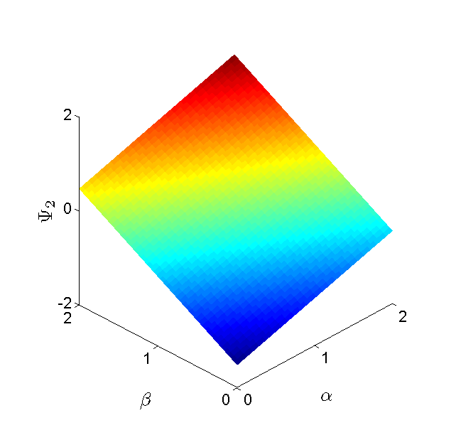
(b) order 1, $\varrho=-0.5$

(c) order 0, $\varrho=0$

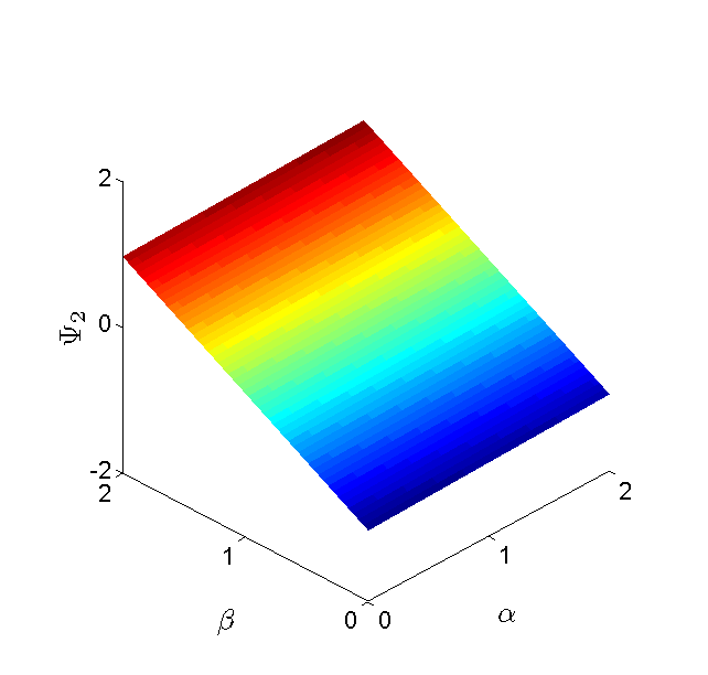
(d) order 1, $\varrho=0$

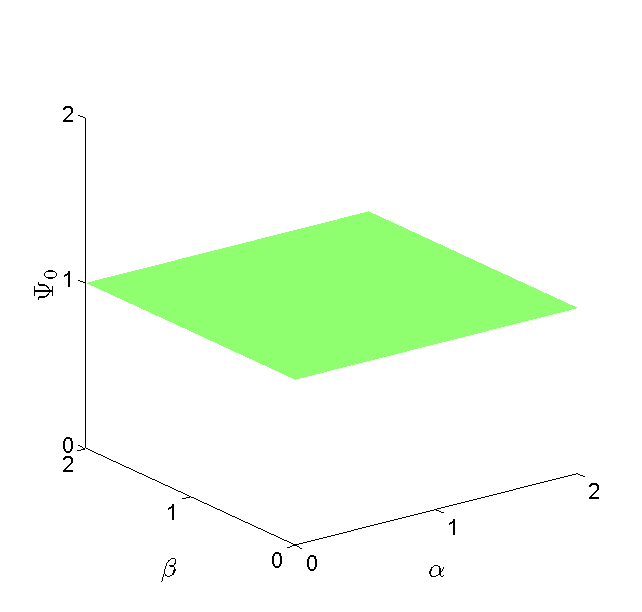
(e) order 0, $\varrho=0.5$

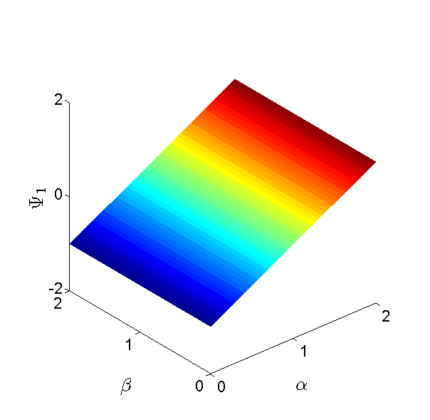
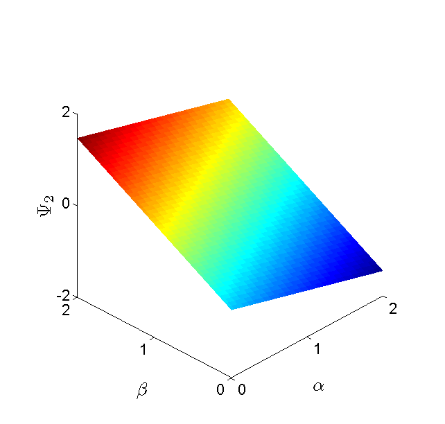
(f) order 1, $\varrho=0.5$

Figure 1. Polynomial basis. Order 0 and 1, for $\varrho=\{0,\pm 0.5\}$

(a)

(b) order 2, $\varrho=-0.5$

(c)

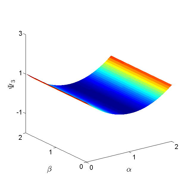
(d)

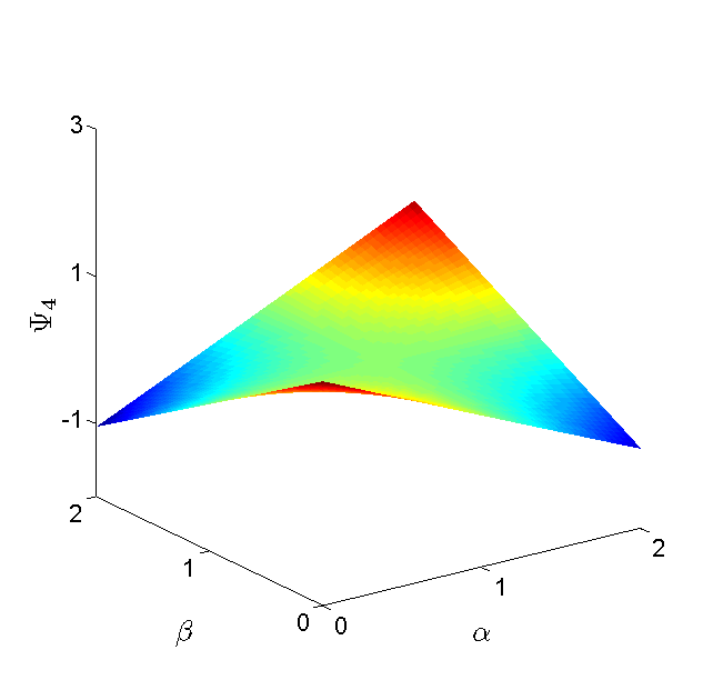
(e) order 2, $\varrho=0$

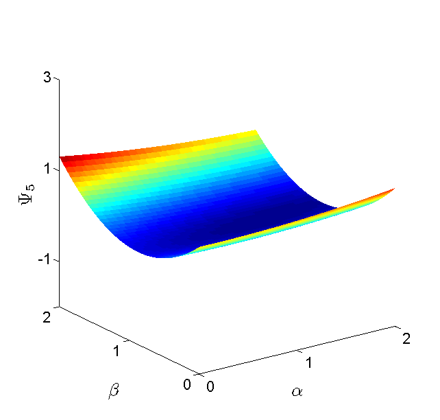
(f)

(g)

(h) order 2, $\varrho=+0.5$

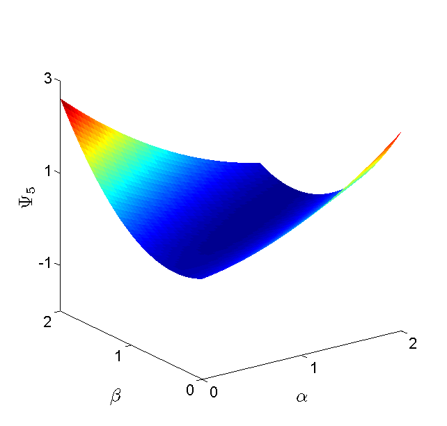
(i)

Figure 2. Polynomial basis. Order 2, for $\varrho=\{0,\pm 0.5\}$

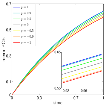
(a) Mean

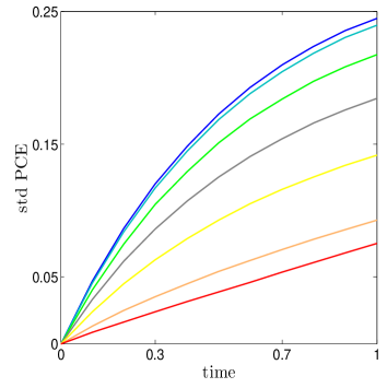
(b) Standard deviation

Figure 3. Effect of correlation on mean and standard deviation of decay equation (29)

Figures 1-2 show all polynomials of order 0, 1 and 2 for correlation coefficients $\varrho=\{0,\pm 0.5\}$. The plots show clearly the non-uniqueness of the orthogonal basis, viz., the influence of the ordering of the monic polynomials (7): the first polynomials of a new order, $\Phi_{\{0,1,3\}}$, are independent of the correlation coefficient and only determined by the first monic polynomial $e_{\{0,1,3\}}$ of that order, the next ones of the same order, $\Phi_{\{2,4,5\}}$, are different and dependent on the correlation. In Figure 3 we show the stochastic mean and standard deviation of the solution of Eq. (29) for the seven values of the correlation coefficient using a PCE expansion of 45 terms, which corresponds to a polynomial order of 8 and the polynomial basis calculated with the proposed method. The results are plot accurate, in the cases of no or full correlation with the ones obtained with the Hermite polynomial basis and same order, and with Monte Carlo simulations for the correlated distributions. The importance of propagating the true input distribution is especially seen in the standard deviation, where neither uncorrelated nor fully correlated give a reasonable approximation for a distribution with correlation $\pm 0.5$. This is also reflected in the Sobol’ indices. Figure 4 shows for all correlation coefficients the evolution of the Sobol’ indices (18) over time and the decomposition into the uncorrelated (19) and the correlated (20) part. These plots and Table 1 show how nicely the contributions of the variables itself and of the correlated variables follow the strength and sign of the correlation coefficient $\varrho$.
Remark. The fully correlated and uncorrelated results do not necessarily bound the correlated ones. E.g., for a delta function response which is located just off the diagonal, full correlation results in a zero variance, and no correlation gives a lower variance than correlation.

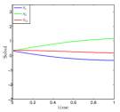
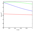
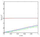
$\varrho=-0.9$

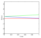
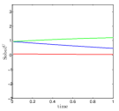
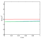
$\varrho=-0.5$

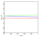
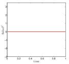
$\varrho=0$

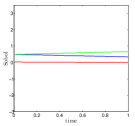
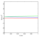
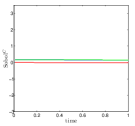
$\varrho=0.5$

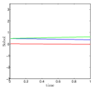
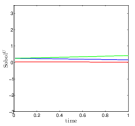
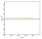
$\varrho=0.9$

Figure 4. Dynamic plots of the Sobol’ indices of decay equation (29). Left: Sobol’ index, middle: contribution from the respective variables, right: contribution due to correlation with other variables.

$\varrho$		$S_{i}$	$S_{i}^{u}$	$S_{i}^{c}$
	$S_{1}$	-0.337996430555719	1.079010380744548	-1.417006811300311
-0.9	$S_{2}$	1.169072254592321	2.794020096839133	-1.624947842246789
	$S_{12}$	0.168924175966794	0.134133434465047	0.034790741501840
	Sum	1.000000000003396	4.007163912048728	-3.007163912045260
	$S_{1}$	0.125070219450471	0.462450913298287	-0.337380693847799
-0.5	$S_{2}$	0.819760985060438	1.197491238203163	-0.377730253142723
	$S_{12}$	0.055168795489075	0.037711983172792	0.017456812316329
	Sum	0.999999999999984	1.697654134674242	-0.697654134674193
	$S_{1}$	0.273826682991019	0.273826682991019	0.000000000000004
0	$S_{2}$	0.709059149322051	0.709059149322055	-0.000000000000000
	$S_{12}$	0.017114167686936	0.017114167686939	0.000000000000015
	Sum	1.000000000000006	1.000000000000013	0.000000000000019
	$S_{1}$	0.340423008768462	0.196827595099748	0.143595413668727
0.5	$S_{2}$	0.660699595355148	0.509674242072905	0.151025353282240
	$S_{12}$	-0.001122604123609	0.016050907606319	-0.017173511729914
	Sum	1.000000000000001	0.722552744778972	0.311794278680881
	$S_{1}$	0.374323408284474	0.161822550653440	0.212500857631028
0.9	$S_{2}$	0.636757390356394	0.419027897208577	0.217729493147815
	$S_{12}$	-0.011080798640891	0.020103679953051	-0.031184478593928
	Sum	0.999999999999977	0.600954127815068	0.399045872184915

Table 1. Sobol’ indices and the contributions from variables itself and from correlated variables in the final timepoint $t_{f}=1$. The respective contributions follow nicely the strength and sign of the correlation coefficient.

To answer the question whether the method has the same favourable convergence behavior as the original expansion for independent normal random variables (cf. [4]), we have performed an error convergence study using the following error measures

(32) $$\varepsilon_{\mu}(p)=\left|\mu_{p}(t_{f})-\mu_{exact}(t_{f})\right|,\qquad\varepsilon_{\sigma}(p)=\left|\sigma_{p}(t_{f})-\sigma_{exact}(t_{f})\right|,$$

where $t_{f}=1$ is the final time point, $\mu_{p}$ and $\sigma_{p}$ correspond to the mean and the standard deviation obtained with PC expansion of order $p$, and $\mu_{exact}$ and $\sigma_{exact}$ are the reference solutions, in this case obtained with $p=8$.

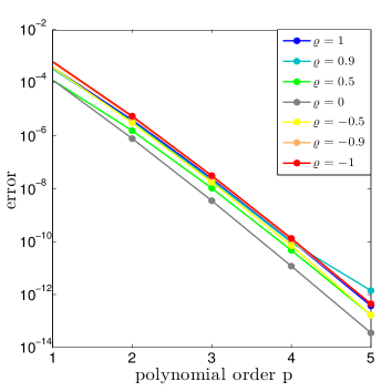
(a) Mean

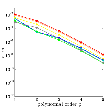
(b) Standard Deviation

Figure 5. Convergence of the error in mean and standard deviation for the decay equation (29)

As we can see in Figure 5 the convergence rate of the error for increasing expansion order is for all correlation coefficients $\varrho$ the same, showing that the convergence rate of the original PCE method for independently normally distributed input variables is conserved.

3.2. Enzymatic reaction

Consider the canonical enzymatic reaction

$$\textrm{E}+\textrm{S} \quad\mathop{\rightleftarrows}\limits^{k_{1}}_{k_{2}}\quad$$ C

C $$\quad\mathop{\rightarrow}\limits^{k_{3}}\quad \textrm{E}+\textrm{P}$$

where the concentrations of the substrate S, the enzyme E, the complex C, and the product P are the state variables and $k_{1}$, $k_{2}$, and $k_{3}$ are the kinetic rate constants. This example has been used in a previous paper [2] to show the effect of noisy data on the reliability of the estimated parameters using linear regression. However, in most cases biologists are not so much interested in accurate model parameters, but in an accurate solution of the QoI, in this case the concentration of the product P. We now can propagate the uncertainty in the parameters, given by the Fisher information matrix, so including correlation between the kinetic parameters, through the model to obtain the pdf for the QoI [P]. The mathematical model for this enzymatic reaction is given by the following system of ODEs:

$$\frac{d[\textrm{{S}}](t)}{dt} = -k_{1}[\textrm{{E}}](t)[\textrm{{S}}](t)+k_{2}[\textrm{{C}}](t)$$

$$\frac{d[\textrm{{C}}](t)}{dt} = k_{1}[\textrm{{E}}](t)[\textrm{{S}}](t)-k_{2}[\textrm{{C}}](t)-k_{3}[\textrm{{C}}](t)$$

(33) $$\frac{d[\textrm{{E}}](t)}{dt} = -k_{1}[\textrm{{E}}](t)[\textrm{{S}}](t)+k_{2}[\textrm{{C}}](t)+k_{3}[\textrm{{C}}](t)$$

$$\frac{d[\textrm{{P}}](t)}{dt} = k_{3}[\textrm{{C}}](t)$$

Data for [C] are available at regular intervals during the time interval [0,20] and the initial concentrations are known $[\textrm{{S}}](0)=1$, $[\textrm{{C}}](0)=0$, $[\textrm{{E}}](0)=1$, and $[\textrm{{P}}](0)=0$. The parameters $k_{1}$, $k_{2}$, and $k_{3}$ have been obtained by linear regression using the noisy data for [C]. The optimal value of the parameters in [2] was ${\boldsymbol{k}}=(0.683,0.312,0.212)$, with (independent) confidence intervals $\Delta=[0.033,0.028,0.005]$. To study the propagation of the uncertainty through the model, the parameters are assumed to be random and their pdf is built based on the results in [2]. Thus, we assumed that the parameters follow a uniform distribution with mean the optimal value of the parameters ${\boldsymbol{\mu}}=(0.683,0.312,0.212)$, standard deviation ${\boldsymbol{\sigma}}=(0.206,0.175,0.031)$ based on the amplitude of the confidence intervals (with multiplication factor limited to 6.25 to avoid entering the non-physical negative parameter space), and $C$ the correlation matrix also obtained from the Fisher information matrix; as in the previous example, the fully correlated case, $C_{f}$, and the uncorrelated case, $C_{u}$, are also studied

$$C=\begin{pmatrix}1&0.9&-0.37\\ 0.9&1&-0.45\\ -0.37&-0.45&1\\ \end{pmatrix}\;C_{f}=\begin{pmatrix}1&1&-1\\ 1&1&-1\\ -1&-1&1\\ \end{pmatrix}\;C_{u}=\begin{pmatrix}1&0&0\\ 0&1&0\\ 0&0&1\\ \end{pmatrix}\$$

As the analytic expression for the pdf of the joint distribution of two or more correlated uniform variables is unknown, we cannot use the moment-generating function to calculate all the required moments. Therefore, Monte Carlo integration will be used in this example. To generate sampling points from a correlated multidimensional uniform distribution we used the standard approach of computing them from the correlated normal distribution (see, e.g., [6]). Again, the problem collapses to one-dimensional in the fully correlated case, correlation matrix $C_{f}$. The only parameter in this case follows the standard uniform distribution $\mathcal{U}(0,1)$.

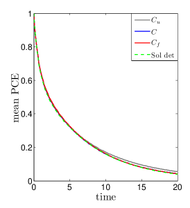
(a) [S]

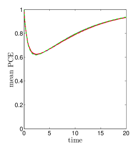
(b) [E]

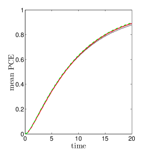
(c) [P]

Figure 6. Mean of the stochastic state variables of Eq. (3.2).

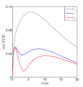
(a) [S]

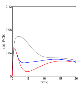
(b) [C] and [E]

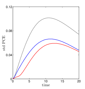
(c) [P]

Figure 7. Standard deviation of the stochastic state variables of Eq. (3.2) for the uncorrelated case (grey), the fully correlated case (red), and the correlation matrix resulting from the experimental errors (blue).

For all three cases - correlated, uncorrelated, and fully correlated - we applied PCE with Galerkin projection to Eq. (3.2).

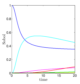
(a) [S]

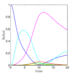
(b) [C] and [E]

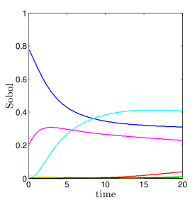
(c) [P]

Figure 8. Dynamic plots of the Sobol’ indices of the enzymatic reaction (3.2) for the uncorrelated case.

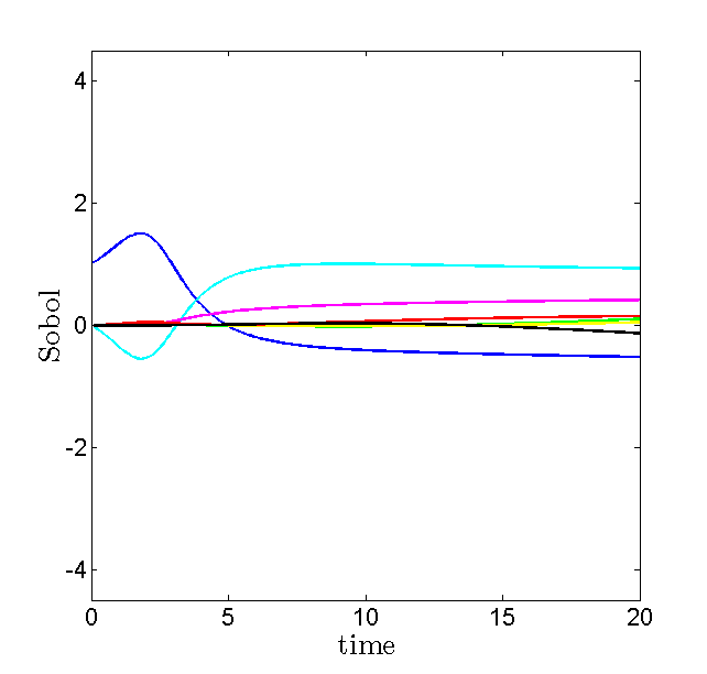
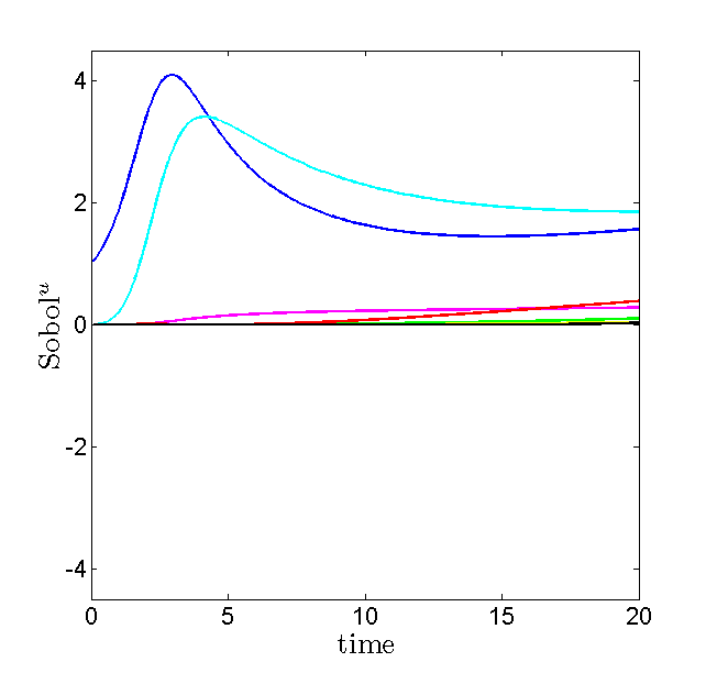
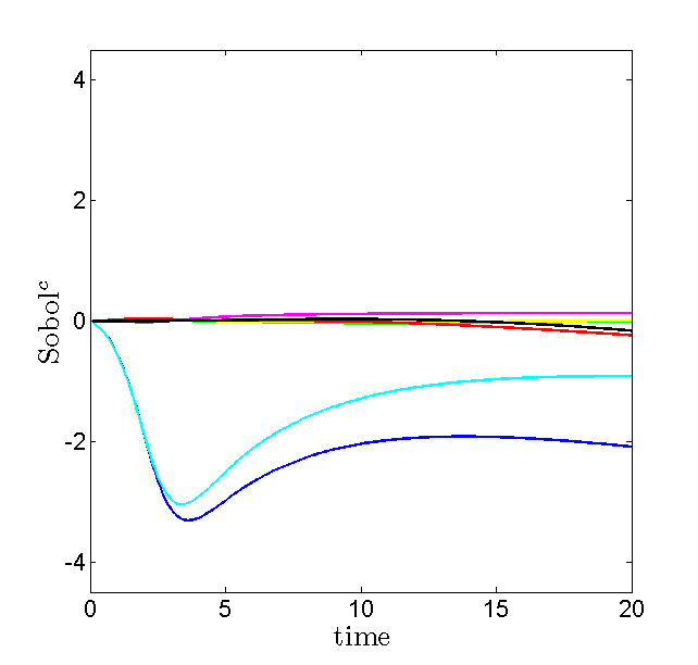
[S]

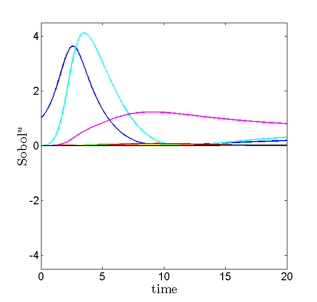
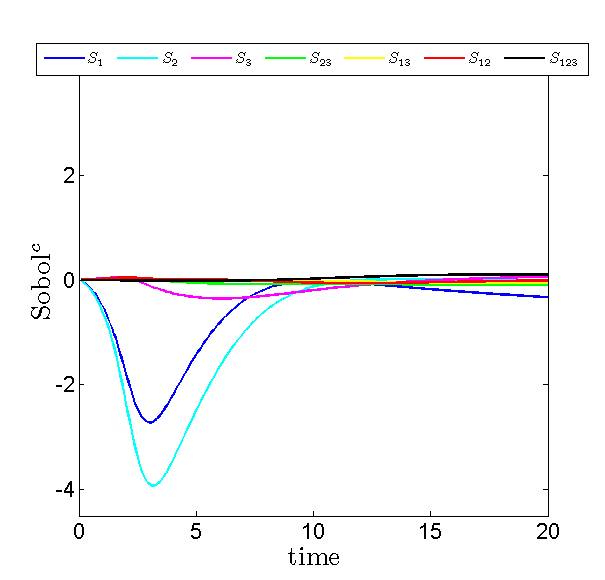
[C] and [E]

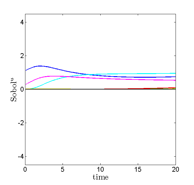
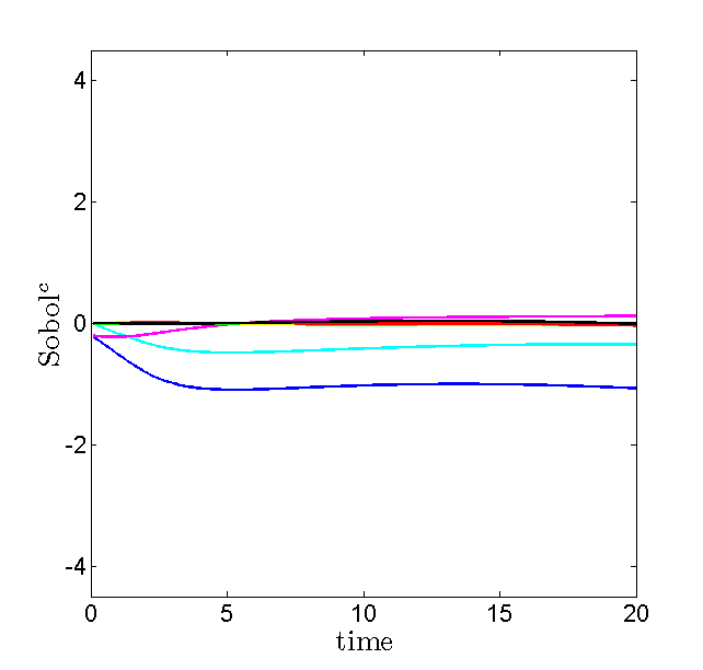
[P]

Figure 9. Dynamic plots of the Sobol’ indices of enzymatic reaction (3.2), for the correlation matrix resulting from the experimental errors. Left: Sobol’ index $S$, middle: contribution from the respective variables, $S^{u}$, right: contribution due to correlation with other variables, $S^{c}$.

Figures 6 and 7 show the obtained mean and standard deviation of all concentrations, respectively. Note, that the concentration of the complex C has an equal dynamic behaviour - with opposite sign - as that of the enzyme E. Again, it can be clearly seen from Fig. 7 that the amount of correlation between the random parameters has a significant impact on the variance of the stochastic state variables. Without correlation the pre-equilibrium dynamics are seen only in the complex C, and as a consequence in the enzyme E, whereas the dynamics of the variance in the product P simply follow those of the substrate S. With correlation the pre-equilibrium dynamics show up also in the substrate S. This difference is displayed too in the evolution of the Sobol’ indices over time, see Figs. 8 and 9 (left column). From the plots in Fig. 9 it is again obvious that the interpretation of the Sobol’ indices - and thus the ranking of the random variables - is less clear in case of correlated random variables. First of all, the Sobol’ indices are no longer positive, and secondly, the contribution due to correlation can completely cancel the contribution from the variable itself, resulting in a small Sobol’ value, but fixing such a variable would have a large impact on the outcome.

[S]	$S_{i}$	$S_{i}^{\mathrm{u}}$	$S_{i}^{\mathrm{c}}$	$S_{i}$	$S_{i}^{\mathrm{u}}$	$S_{i}^{\mathrm{c}}$
$S_{1}$	0.35	0.36	-0.01	-0.52	1.57	-2.09
$S_{2}$	0.45	0.46	-0.01	0.93	1.85	-0.92
$S_{3}$	0.08	0.08	-0.00	0.42	0.28	0.13
$S_{23}$	0.02	0.02	-0.00	0.10	0.10	0.00
$S_{13}$	0.00	0.00	-0.00	0.05	0.04	0.00
$S_{12}$	0.09	0.09	-0.00	0.15	0.39	-0.24
$S_{123}$	0.00	0.00	0.00	-0.13	0.03	-0.16
Sum	0.99	1.01	-0.02	1.00	4.26	-3.28
[C] & [E]	$S_{i}$	$S_{i}^{\mathrm{u}}$	$S_{i}^{\mathrm{c}}$	$S_{i}$	$S_{i}^{\mathrm{u}}$	$S_{i}^{\mathrm{c}}$
$S_{1}$	0.17	0.17	-0.00	-0.14	0.19	-0.33
$S_{2}$	0.24	0.24	-0.00	0.28	0.31	-0.03
$S_{3}$	0.58	0.58	-0.00	0.87	0.80	0.06
$S_{23}$	0.00	0.00	-0.00	-0.08	0.01	-0.08
$S_{13}$	0.00	0.00	0.00	-0.06	0.00	-0.06
$S_{12}$	0.00	0.00	0.00	-0.01	0.00	-0.01
$S_{123}$	0.00	0.00	0.00	0.12	0.02	0.10
Sum	0.99	0.99	0.00	0.98	1.33	-0.35
[P]	$S_{i}$	$S_{i}^{\mathrm{u}}$	$S_{i}^{\mathrm{c}}$	$S_{i}$	$S_{i}^{\mathrm{u}}$	$S_{i}^{\mathrm{c}}$
$S_{1}$	0.31	0.31	-0.00	-0.33	0.75	-1.08
$S_{2}$	0.41	0.41	-0.00	0.61	0.95	-0.34
$S_{3}$	0.23	0.23	-0.00	0.66	0.54	0.12
$S_{23}$	0.01	0.01	-0.00	0.01	0.03	-0.02
$S_{13}$	0.00	0.00	0.00	-0.00	0.01	-0.01
$S_{12}$	0.04	0.04	-0.00	0.05	0.09	-0.04
$S_{123}$	-0.00	0.00	-0.00	-0.00	0.00	-0.00
Sum	1.00	1.00	-0.00	1.00	2.37	-1.37

Table 2. Sobol’ indices in the final time point $t_{f}=20$. The left part of the table corresponds to the uncorrelated case, correlation matrix $C_{u}$; the right part to the correlation matrix $C$ obtained from the FIM. The columns $S_{i}^{u}$ show the contribution from the variables itself and the columns $S_{i}^{c}$ the contribution from correlated variables; with exact computations the $S_{i}^{c}$-column in the left part of the table should be zero.

[S]	$S_{T_{i}}$	$S_{T_{i}}^{\mathrm{u}}$	$S_{T_{i}}^{\mathrm{c}}$	$S_{T_{i}}$	$S_{T_{i}}^{\mathrm{u}}$	$S_{T_{i}}^{\mathrm{c}}$
$S_{T_{1}}$	0.44	0.45	-0.01	-0.45	2.03	-2.49
$S_{T_{2}}$	0.56	0.57	-0.01	1.05	2.37	-1.32
$S_{T_{3}}$	0.10	0.10	0.00	0.44	0.45	-0.03
[C] & [E]	$S_{T_{i}}$	$S_{T_{i}}^{\mathrm{u}}$	$S_{T_{i}}^{\mathrm{c}}$	$S_{T_{i}}$	$S_{T_{i}}^{\mathrm{u}}$	$S_{T_{i}}^{\mathrm{c}}$
$S_{T_{1}}$	0.17	0.17	-0.00	-0.09	0.21	-0.30
$S_{T_{2}}$	0.24	0.24	-0.00	0.31	0.34	-0.02
$S_{T_{3}}$	0.58	0.58	0.00	0.85	0.83	0.02
[P]	$S_{T_{i}}$	$S_{T_{i}}^{\mathrm{u}}$	$S_{T_{i}}^{\mathrm{c}}$	$S_{T_{i}}$	$S_{T_{i}}^{\mathrm{u}}$	$S_{T_{i}}^{\mathrm{c}}$
$S_{T_{1}}$	0.35	0.35	-0.00	-0.28	0.85	-1.13
$S_{T_{2}}$	0.46	0.46	-0.00	0.67	1.07	-0.38
$S_{T_{3}}$	0.24	0.24	0.00	0.67	0.58	0.09

Table 3. Total Sobol’ indices in the final time point $t_{f}=20$. The left part of the table corresponds to the uncorrelated case, correlation matrix $C_{u}$; the right part to the correlation matrix $C$ obtained from the FIM.

Ranking variables is often done based on the Sobol’ indices. Depending on the time-frame of interest, one can use as measure, e.g., the integral over time of the Sobol’ indices, or the Sobol’ indices in a specific point. As an example of the latter we study at the final time-point, $t_{f}=20$, which part of the variance of the concentrations is due to the variance of respective input variables. Tables 2 and 3 give the Sobol’ indices and the total Sobol’ indices, respectively, for the random variables $k_{1}$, $k_{2}$, and $k_{3}$. Note that the sum of the Sobol’ indices equals one and for the uncorrelated case the $S^{c}$ values should be zero, so the deviation of these values gives the error in the approximation, in this case mostly due to the approximation of the high-order moments needed for the Sobol’ indices. From Table 3 one can deduce that, in the uncorrelated case, decomposing the variance of the concentration of the substrate S  would lead to the conclusion that the random variable $k_{3}$ can be fixed to the nominal deterministic value, since its influence on the variance of S is negligible. In the correlated case, however, this is no longer true. One can also see that especially for $k_{1}$ and $k_{2}$ the interpretation of the Sobol’ indices is not trivial, e.g., for C the influence of $k_{1}$ is very small but this is due to cancellation of the $S^{u}$ and $S^{c}$ contribution. As stated before, the interpretation of the Sobol’ indices for correlated random variables is largely an open issue, but it is clear that in general less random input variables can be fixed to their nominal deterministic values.

4. Discussion and concluding remarks

In this paper we extended the PCE method to general multivariate distributions, including correlations between the random input variables, by constructing an orthogonal polynomial basis for the probability space. We showed that the usual statistics like mean, variance and Sobol’ indices can be obtained with no extra cost, as is the case for the current PCE implementations. This method makes it possible to compute for a set of random input variables with any multivariate distribution, including an experimentally determined one, the stochastic distribution of a Quantity of Interest. An application we studied is the true propagation of experimental errors through the parameter-fitting process onto the state variables, so that a QoI based on these state variables is described as a distribution and, e.g., optimal experimental design can be applied to reduce the variance in such a QoI. In this paper we used either exact integration or Monte Carlo to compute the moments and the projection onto the polynomial basis, but for the latter Gauss quadrature is under development.

There are a few remarks to make with respect to the method

• As for other PCE methods, the polynomial base is only dependent on the multivariate distribution of the random input variables. Once computed, all problems with random input variables described by this pdf can be solved using the same base.

• To obtain the polynomial basis raw moments are needed which have to be computed accurately enough not to pollute the results. This is not a trivial task for high dimensional problems or a high polynomial order. E.g., in our first example, the size of the moments range in order of magnitude from 1 for the first ten orders to $10^{15}$ for order 75 for an uncorrelated Normal distribution. If the correlation coefficient $\varrho$ equals $0.9$ the latter order of magnitude is even much higher: $10^{21}$ for moments of order 75.

• The orthogonal polynomial basis is not unique, it is dependent on the choice and ordering of the original set of linearly independent polynomials. It is an open question at the moment whether there is an optimal choice for this original set of polynomials, e.g., to reduce the magnitude of the moments required or to simplify computations.

• Whereas in the uncorrelated case interpretation of Sobol’ indices and ranking of the influence of the variation of the random input variables on the variance in the QoI is more or less straighforward, this is no longer true for correlated random variables.

References

- [1] H.L. Anderson, Metropolis, Monte Carlo and the MANIAC, Los Alamos Science, 14, 96-108, 1986.
- [2] M. Ashyraliyev, Y. Fomekong-Nanfack, J.A. Kaandorp, J.G. Blom, Systems biology: parameter estimation for biochemical models, The FEBS Journal, 276(4), 886-902, 2009.
- [3] A.J. Brown, Enzyme action, J. Chem. Soc. 81, 373-386, 1902.
- [4] R. Cameron, W. Martin, The orthogonal development of nonlinear functionals in series of Fourier-Hermite functionals, Annals of Mathematics, 48, 385-392, 1947.
- [5] J.L. Castro, M. Navarro, J.M. Sánchez, J.M. Zurita, Loss and gain functions for CBR retrieval, Information Sciences, 179(11), 1738-1750, 2009.
- [6] C.T.S. Dias, A. Samaranayaka, B. Manly, On the use of correlated beta random variables with animal population modelling, Ecological Modelling, 215, 293-300, 2008.
- [7] M.S. Eldred, C.G. Webster, P.G. Constantine, Evaluation of non-intrusive approaches for Wiener-Askey generalized polynomial chaos, AIAA 2008-1892, 2008.
- [8] B. Fox, Strategies for Quasi-Monte Carlo, Kluwer academic Pub., 1999.
- [9] V. Golosnoy, Y. Okhrin, General uncertainty in portfolio selection: A case-based decision approach, Journal of Economic Behavior & Organization, 67, (3-4), 718-734, 2008.
- [10] G.H. Golub, C.F. van Loan, Matrix computations (third edition), The John Hopkins University Press, Baltimore and London, 1996.
- [11] T.Y. Hou, W. Luo, B. Rozovskii, H.-M. Zhou, Wiener chaos expansions and numerical solutions of randomly forced equations of fluid mechanics, Journal of Computational Physics, 216(2), 687-706, 2006.
- [12] F.S. Hover, M.S. Triantafyllou, Application of polynomial chaos in stability and control, Automatica, 42(5), 789-795, 2006.
- [13] M. Kleiber, T.D. Hien, The stochastic finite element method: basic perturbation technique and computer implementation, Wiley, 1992.
- [14] R.H. Kraichnan, Direct-interaction approximation for a system of several interacting simple shear waves, The Physics of Fluids, 6(11), 1603-1609, 1963.
- [15] G. Li, H. Rabitz, P.E. Yelvington, O.O. Oluwole, F. Bacon, C.E. Kolb, J. Schoendorf, Global sensitivity analysis for systems with independent and/or correlated inputs, The Journal of Physical Chemistry A, 114(19), 6022-6032, 2010.
- [16] H. Li, D. Zhang, Probabilistic collocation method for flow in porous media: comparisons with other stochastic methods, Water Resources Research, 43, 44-48, 2009.
- [17] W. Loh, On Latin hypercube sampling, Annals of Statistics, 24, 2058-2080, 1996.
- [18] J.L. Lumley, The structure of inhomogeneous turbulent flows, In Atmospheric Turbulence and Wave Propagation, ed. A.M. Yaglom, V.I. Tatarski, 166-178, 1967.
- [19] N. Madras, Lectures on Monte Carlo methods, American Mathematical Society, Providence, RI, 2002.
- [20] MATLAB and Symbolic Math Toolbox Release 2012b, The MathWorks, Inc., Natick, Massachusetts, United States.
- [21] H.N. Najm, Uncertainty quantification and polynomial chaos techniques in computational fluid dynamics, Annual Review of Fluid Mechanics, 41, 35-52, 2009.
- [22] A. Nataf, Détermination des distributions de probabilités dont les marges sont données, Comptes Rendus de l’Académie des Sciences, 225, 42-43, 1962.
- [23] S. Oladyshkin, W. Nowak, Data-driven uncertainty quantification using the arbitrary polynomial chaos expansion, Reliability Engineering & System Safety, 106, 179-190, 2012.
- [24] S.A. Orszag, L.R. Bissonnette, Dynamical properties of truncated Wiener-Hermite expansions, The Physics of Fluids, 10(12), 2603-2613, 1967.
- [25] A.B. Owen, Variance components and generalized Sobol’ indices, SIAM/ASA J. Uncertainty Quantification 1(1), 19-41, 2013.
- [26] M. Rajaschekhar, B. Ellingwood, A new look at the response surface approach for reliability analysis, Structural Safety, 123, 205-220, 1993.
- [27] M. Rosenblatt, Remarks on a multivariate transformation, The Annals of Mathematical Statistics, 23(3), 470-472, 1952.
- [28] E. Schmidt, Zur Theorie der linearen und nichtlinearen Integralgleichungen. I. Teil: Entwicklung willkürlicher Funktionen nach Systemen vorgeschriebener, Math. Ann., 63, 433-476, 1907.
- [29] P. Schola, O.P. Le Maitre, Polynomial chaos expansion for subsurface flows with uncertain soil parameters, Advances in Water Resources, 62, Part A, 139-154, 2013.
- [30] C. Soize, R. Ghanem, Physical systems with random uncertainties: chaos representations with arbitrary probability measure, SIAM Journal on Scientific Computing, 26(2), 395-410, 2004.
- [31] I.M. Sobol’, Sensitivity estimates for nonlinear mathematical models, Math. Modeling & Comput. Exp., 1, 407-414, 1993.
- [32] B. Sudret, Global sensitivity analysis using polynomial chaos expansions, Reliability Engineering & System Safety, 93(7), 964-979, 2008.
- [33] H. Hotelling, M.R. Pabst, Rank correlation and test of significance involving no assumption of normality, Annals of Mathematical Statistic, 7, 29-43, 1936.
- [34] M. Villegas, F. Augustin, A. Gilg, A. Hmaidi, U. Wever, Application of the polynomial Cchaos expansion to the simulation of chemical reactors with uncertainties, Mathematics and Computers in Simulation, 82(5), 805-817, 2012.
- [35] X. Wan, G.E. Karniadakis, Beyond Wiener-Askey expansions: handling arbitrary PDFs, Journal of Scientific Computing, 27(1-3), 455-464, 2006.
- [36] N. Wiener, The homogeneous chaos, American Journal of Mathematics, 60(4), 897-936, 1938.
- [37] J.A.S. Witteveen, H. Bijl, Efficient quantification of the effect of uncertainties in advection-diffusion problems using polynomial chaos, Numerical Heat Transfer B: Fundamentals, 53, 437-465, 2008.
- [38] J.A.S. Witteveen, S. Sarkar, H. Bijl, Modeling physical uncertainties in dynamic stall induced fluid-structure interaction of turbine blades using arbitrary polynomial chaos, Computers and Structures, 85, 866-878, 2007.
- [39] J.A.S. Witteveen, H. Bijl, Modeling arbitrary uncertainties using Gram-Schmidt polynomial chaos, AIAA-2006-896, 44th AIAA Aerospace Sciences Meeting and Exhibit, Reno, Nevada, 2006.
- [40] D. Xiu, Efficient collocational approach for parametric uncertainty analysis, Communications in Computational Physics, 2(2), 293-309, 2007.
- [41] D. Xiu, G.E. Karniadakis, The Wiener–Askey polynomial chaos for stochastic differential equations, SIAM Journal on Scientific Computing, 24(2), 619-644, 2002.