Fluid structure in the immediate vicinity of an equilibrium three-phase contact line and assessment of disjoining pressure models using density functional theory

Abstract

We examine the nanoscale behavior of an equilibrium three-phase contact line in the presence of long-ranged intermolecular forces by employing a statistical mechanics of fluids approach, namely density functional theory (DFT) together with fundamental measure theory (FMT). This enables us to evaluate the predictive quality of effective Hamiltonian models in the vicinity of the contact line. In particular, we compare the results for mean field effective Hamiltonians with disjoining pressures defined through (I) the adsorption isotherm for a planar liquid film, and (II) the normal force balance at the contact line. We find that the height profile obtained using (I) shows good agreement with the adsorption film thickness of the DFT-FMT equilibrium density profile in terms of maximal curvature and the behavior at large film heights. In contrast, we observe that while the height profile obtained by using (II) satisfies basic sum rules, it shows little agreement with the adsorption film thickness of the DFT results. The results are verified for contact angles of $20^{\circ}$, $40^{\circ}$ and $60^{\circ}$.

I Introduction

Consider a droplet sitting on a substrate and surrounded by its saturated vapor. In the partial wetting regime, the droplet’s surface meets the substrate at a finite contact angle. Macroscopically, this contact angle is a material constant of the fluid-wall pair. Microscopically, intermolecular forces dictate the exact structure of the fluid in the vicinity of the point where the liquid, the vapor phase and the substrate meet. We study this microscopic structure using elements from the statistical mechanics of fluids and compare our results with two approaches using coarse-grained mean-field Hamiltonian theory.

Understanding the exact structure at a contact line with a finite contact angle is of increasing interest for a wide spectrum of technological applications but also from a fundamental point of view. Recent advances in technology allow the design of devices of increasingly small size, highlighting the importance of developing a fundamental understanding of phenomena at small scales for the manipulation and control of fluids in micro-/nanofluidic devices.Seemann et al. (2005); Rauscher and Dietrich (2008) Small-scale phenomena in wetting are also important in biology, e.g. the rupture of liquid films in the airways of lungs,Jensen and Grotberg (1992) or the rupture of the tearfilm on the eyeball.Wong, Fatt, and Radke (1996) Finally, a well-founded understanding of equilibrium behavior is a prerequisite for the accurate modeling of the dynamic contact line behavior.

The study of the microscopic structure at the contact line is limited by its high computational cost.MacDowell (2011a) Two ways of computing the density structure for equilibrium systems are Monte-Carlo (MC) Herring and Henderson (2010); Das and Binder (2010) and Molecular Dynamics (MD) computations.Werder et al. (2001); Tretyakov et al. (2013) MC and MD solve for the positions of individual particles, such that the number of particles necessarily limits the system size to nanoscales, and despite dramatic improvements in computational power, MC/MD computations are still only applicable for small fluid volumes. As an alternative to particle-based computations, classical density functional theory (DFT) allows to solve directly for the density distribution of inhomogeneous systems Evans (1979); Wu (2006) and retains the microscopic details of macroscopic systems but at a cost much lower to that in MC/MD. In the past, DFT has been predominantly applied to one-dimensional (1D) scenarios Stewart and Evans (2005); Nold, Malijevský, and Kalliadasis (2011) but has recently been used in two-dimensional (2D) scenarios such as nanodrops, Berim and Ruckenstein (2008); Ruckenstein and Berim (2010) critical point wedge filling, Malijevský and Parry (2013) capillary prewetting, Yatsyshin, Savva, and Kalliadasis (2013) and three-dimensional nucleation processes. Zhou, Mi, and Zhong (2012)

Intermolecular interactions between polar and non-polar particles, as well as hydrogen bonds and other interactions, are short-ranged and decay exponentially.Bonn et al. (2009) Physically, however, the much more common occurrence are fluids with apolar, uncharged particles with long-range van der Waals type interactions Béguin et al. (2013) — which appear to be the ‘only general aspect of the physics of wetting that is not well-understood’. Henderson (2005) Fluids with long-range interactions exhibit a different wetting behavior to fluids with short-ranged interactions. Bonn et al. (2009) In addition, the latter are numerically more accessible as they allow for a finite cutoff length for the inter-particle interactions.

Wetting of fluids with long-range dispersion forces has been studied by means of a sharp-kink approximation for the density profile.Dietrich (1988); Bauer and Dietrich (1999); Hofmann et al. (2010) Other studies have relaxed the density profile by using a local density approximation for the hard-sphere inter-particle potential.Pereira and Kalliadasis (2012) However, at present the most successful and accurate DFT for hard-sphere systems with attractive interactions is that of fundamental measure theory (FMT).Roth (2010) DFT-FMT with dispersion forces has been successfully applied in studies of critical point wedge filling Malijevský and Parry (2013) and density computations in the vicinity of liquid wedges. Merath (2008)

Here we construct an equilibrium three-phase contact line of a fluid with dispersion interactions in the immediate vicinity of a wall using an accurate FMT model for the hard-sphere interactions. This allows us to solve for the density profile of the fluid in the contact line region and to shed light on the fluid structure there down to the nanoscale: In particular, we observe the fluid structure there down to the nanoscale: in particular, we observe the presence of a step-like structure for the higher fluid densities very close to the contact line. The DFT-FMT approach also allows us to test mean-field effective Hamiltonian approaches which reduce the dimension of the system by one, describing the interface by a simple height profile. In general, the Hamiltonian of such systems is written as a sum of the contribution due to the liquid-vapor interface and an effective interface potential.Lipowsky and Fisher (1987); Mikheev and Weeks (1991)

The interface potential goes back to the concept of disjoining pressure introduced by Derjaguin Derjaguin (1987); Derjaguin and Churaev (1986) and Frumkin Frumkin (1938) (but we note that Derjaguin’s work was published earlier Derjaguin and Obuchov (1936)). The disjoining pressure is defined as the excess pressure acting on a substrate due to the presence of a thin liquid film, and it was directly linked with the adsorption isotherm, the plot of the film thickness against the chemical potential of the system. Later, Dzyaloshinskii, Lifshitz and Pitaevskii (DLP) directly computed the disjoining pressure from the dispersion interactions.Dzyaloshinskii, Lifshitz, and Pitaevskii (1961) This connection between the definitions of disjoining pressure, as well as its applicability to nonplanar systems in the framework of an effective Hamiltonian theory, was recently analyzed in a number of discussion papers that appeared in Eur. Phys. J.: Spec. Top., special issue ‘Wetting and Spreading Science - quo vadis?’.MacDowell (2011a); Henderson (2011a); MacDowell (2011b); Henderson (2011b, c) In particular, the transferability and/or universality, of results using disjoining pressure in an effective Hamiltonian approach, as well as the validity of the different definitions of the disjoining pressure were questioned in these papers.

In this work, we make progress towards addressing these questions by employing a DFT-FMT framework for a system with long-range wall-fluid and fluid-fluid interactions. In particular, we study and directly compare two routes to the disjoining pressure. First, we compute the adsorption isotherm employing DFT in a planar configuration. Using an effective Hamiltonian approach, this allows us to define a specific height profile across the contact line. Secondly, we compute the full density distribution of a three-phase contact line. This exact result can be used to define a disjoining pressure based on the normal force balance,Herring and Henderson (2010) in the spirit of a parameter-passing technique. The disjoining pressure containing this information from the 2D density profile is in turn inserted into a Hamiltonian approach to compute a simple height profile.

In Sec. II, we give an overview of the DFT model we employ to solve for the exact density profile in the vicinity of an equilibrium contact line. In Sec. III, we give details of the numerical scheme we developed to solve the DFT equations. A brief introduction to Hamiltonian approaches together with the two definitions of the disjoining pressure considered in this study is given in Sec. IV. In Sec. V we compare the DFT results with the Hamiltonian approaches. Finally, we summarize our results and provide an outlook to future work in Sec. VI.

II DFT Model

We employ classical DFT to study the density distribution in the vicinity of a static contact line. Classical DFT has been of paramount importance for the study of inhomogeneous fluids. It is based on Mermin’s theorem, Mermin (1965) which allows the Helmholtz free energy $\mathcal{F}$ to be written as a unique functional of the number density profile $n({\bf r})$.Wu (2006) It can be shown rigorously that the equilibrium density distribution minimizes the grand potential Evans (1979)

$$\Omega[n]=\mathcal{F}[n]+\int n({\bf r})\left\{V_{\text{ext}}({\bf r})-\mu\right\}\text{d}{\bf r},$$ (1)

where $\mu$ is the chemical potential and $V_{\text{ext}}$ is the external potential. We minimize Eq. (1) by solving the Euler-Lagrange equation

$$\frac{\delta\Omega[n]}{\delta n({{\bf r}})}=0.$$ (2)

For a simple fluid of particles interacting with a Lennard-Jones (LJ) potential, the free energy is usually split into a repulsive hard-sphere part and an attractive contribution

$$\mathcal{F}[n]=\mathcal{F}_{\text{HS}}[n]+\mathcal{F}_{\text{attr}}[n].$$ (3)

We model the hard-sphere contribution with a Rosenfeld FMT approach,Rosenfeld (1989) which accurately models both structure and thermodynamics of hard-sphere fluids.Roth (2010) The attractive interactions are modeled with a mean-field Barker-Henderson approach Barker and Henderson (1967)

$$\mathcal{F}_{\text{attr}}[n] =\frac{1}{2}\iint\phi_{\text{attr}}({|{\bf r}-{\bf r}^{\prime}|})n({\bf r})n({\bf r}^{\prime})\text{d}{\bf r}^{\prime}\text{d}{\bf r},$$ (4)

where the attractive interaction potential is given by

$$\phi_{\text{attr}}\left(r\right)=\varepsilon\left\{\begin{array}[]{ll}0&\text{for }r\leq\sigma\\ 4\left(\left(\frac{\sigma}{r}\right)^{12}-\left(\frac{\sigma}{r}\right)^{6}\right)&\text{for }r>\sigma\end{array}\right..$$ (7)

Here, $\sigma$ is the distance from the center of the particle at which the LJ potential is zero and $\varepsilon$ is the depth of the LJ potential. The simple fluid described by the given model has a critical point at $k_{B}T_{c}=1.0\varepsilon$, where $k_{B}$ is the Boltzmann constant and all computations in this work were performed at $T=0.75T_{c}$, at which the liquid and vapor number densities are well-separated ($n_{\text{liq}}\sigma^{3}=0.622$, $n_{\text{vap}}\sigma^{3}=0.003$) and at which the surface tension becomes $\gamma_{\text{lv}}=0.3463\varepsilon/\sigma^{2}$. All 2D computations are performed at the saturation chemical potential, at which the bulk vapor and bulk liquid are equally stable. A phase diagram of the model used in this work is depicted in Fig. 1, and compared with experimental and simulation results for argon. Michels, Levelt, and Graaff (1958); Trokhymchuk and Alejandre (1999) We note that the discrepancy between the data stems from the fact that argon is not well modeled with a Barker-Henderson interaction potential. For a DFT model which reproduces more accurately the bulk properties of argon, see e.g. Peng and Yu. Peng and Yu (2008)

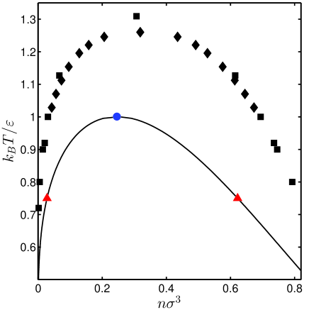
Figure 1: Bulk phase diagram for values at saturation. The solid line represents the phase diagram for the model used in this work. The circle denotes the critical point at $\{k_{B}T_{c}=1.0\varepsilon,n_{c}\sigma^{3}=0.246\}$; the triangles denote the vapor and liquid densities for the temperature of $T=0.75T_{c}$ at which all computations in this work are done. The black squares denote experimental results for argon ($\sigma=3.405\times 10^{-8}\text{cm}$ and $\varepsilon=165.3\times 10^{-16}\text{erg}$) by Michels, Levelt, and De Graaff. Michels, Levelt, and Graaff (1958) The black diamonds represent canonical MD simulations by Trokhymchuk and Alejandre. Trokhymchuk and Alejandre (1999)

The external potential is derived from the interaction of the wall-fluid particles, modeled analogously to the fluid-fluid interaction as

$$\phi_{\text{attr}}^{\text{wf}}\left(r\right)=\varepsilon_{\text{w}}\left\{\begin{array}[]{ll}\infty&\text{for }r\leq\sigma\\ 4\left(\left(\frac{\sigma}{r}\right)^{12}-\left(\frac{\sigma}{r}\right)^{6}\right)&\text{for }r>\sigma\end{array}\right.,$$ (10)

where $\varepsilon_{\text{w}}$ is the depth of the wall-fluid interactions. Consider a Cartesian coordinate system with the $x$-$z$ plane parallel to the wall and the $y$-coordinate direction normal to the wall. The external potential is then obtained from the integration of the interactions over the uniform density distribution of wall particles $n_{\text{w}}$ for $y\leq-\sigma$, giving

$$V_{\text{ext}}\left(y\right) =\left\{\begin{array}[]{ll}\infty&y\leq 0\\ \frac{2}{3}\pi\alpha_{\text{w}}\sigma^{3}\left[\frac{2}{15}\left(\frac{\sigma}{y+\sigma}\right)^{9}-\left(\frac{\sigma}{y+\sigma}\right)^{3}\right]&y>0\end{array}\right.,$$ (13)

where $\alpha_{\text{w}}=n_{\text{w}}\varepsilon_{\text{w}}$ is the strength of the wall potential.

III Computations

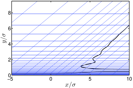
Figure 2: Sketch of part of the grid employed in the numerical computations of this work. The complete grid covers the full half space $y>0$. The gridlines represent isolines of the computational variables $\xi$ and $\eta$, which are mapped to the physical space $(x,y)$ as given in Eqs. (14) and (15). Here we plot every second isoline for a grid with $45$ and $75$ Chebychev collocation points in the $\xi$ and $\eta$ direction, respectively, and with parameters $L_{1}=4\sigma$, $L_{2}=2\sigma$ and angle $\theta_{\text{n}}=40^{\circ}$. The black solid line represents one isoline of a density profile for a contact line computation.

Solving for the full microscopic density profile at the contact line requires a considerable amount of modeling and computational effort, restricting computations to systems of very small size, such as nano-droplets.Berim and Ruckenstein (2008); Ruckenstein and Berim (2010) In the configuration we discuss here, this is circumvented by constructing a liquid wedge (at saturation) in contact with the substrate and with a well-defined three-phase contact line. This effectively allows us to model the contact line of a macroscopic droplet.

In this case, choosing a skewed grid for a representation of our numerical results, such as depicted in Fig. 2, is computationally advantageous. For a map from the computational to the physical domain, we employ a spectral collocation method Trefethen (2000) to represent functions in the half space $y\geq 0$. In particular, we employ a tensor product of two 1D Chebychev grids in $\left(\xi,\eta\right)\in[-1,1]\times[-1,1]$. This domain is mapped onto the half-space through Shen and Wang (2009)

$$x^{\prime}=L_{1}\frac{\xi}{\sqrt{1-\xi^{2}}},\qquad y^{\prime}=L_{2}\frac{1+\eta}{1-\eta},$$ (14)

where $L_{1},L_{2}$ represent the length-scales of the map. The maps are such that half of the collocation points in each direction $\xi$, $\eta$ are mapped onto the intervals $[-L_{1},L_{1}]$ and $[0,L_{2}]$, respectively. In order to efficiently represent density distributions of wedges with relatively small contact angles, the grid is skewed by an angle $\theta_{\text{n}}$, such that

$$x=\frac{x^{\prime}}{\sin\theta_{\text{n}}}+y^{\prime}\cot\theta_{\text{n}},\qquad y=y^{\prime},$$ (15)

where division by $\sin\theta_{\text{n}}$ corrects the scaling of $L_{1}$ in the skewed grid, such that the number of collocation points across a liquid-vapor interface at angle $\theta_{\text{n}}$ is invariant with respect to the angle. We then impose that the density at the collocation points for $y>y_{\text{max}}$ corresponds to a straight wedge with angle $\theta_{\text{n}}$. In other words, the angle of the liquid-vapor interface for $y>y_{\text{max}}$ is imposed as a boundary condition. Also, we consider density profiles which converge smoothly to the planar wall-vapor and wall-liquid equilibrium density profiles as $x\to-\infty$ and $x\to\infty$, respectively.

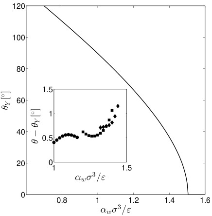
Figure 3: Plot of the contact angle dependence on the strength of the wall attraction $\alpha_{\text{w}}$, computed via Young’s equation (16) from surface tensions as calculated from DFT for planar geometries. Complete wetting is reached at $\alpha_{\text{w}}\sigma^{3}/\varepsilon=1.50$. The inset shows measurements of the contact angle from 2D computations as described in the text with $y_{\text{max}}=15\sigma$ as deviations from the Young contact angle. Circles, squares and diamonds depict computations with $\theta_{\text{n}}=90^{\circ}$, $60^{\circ}$ and $40^{\circ}$, respectively.

Physically, the contact angle $\theta_{\text{Y}}$ of a liquid-vapor interface in contact with a substrate is uniquely defined by the fluid properties and the external potential induced by the substrate through Young’s equation

$$\gamma_{\text{lv}}\cos\theta_{\text{Y}}=\gamma_{\text{wv}}-\gamma_{\text{wl}},$$ (16)

where $\gamma_{\text{lv}}$ is the liquid-vapor surface tension and $\gamma_{\text{wl}}$ and $\gamma_{\text{wv}}$ are the wall-liquid and the wall-vapor surface tensions. In Fig. 3, we plot the Young contact angle as a function of the wall attraction $\alpha_{\text{w}}$, where the surface tensions $\gamma_{\text{lv}}$, $\gamma_{\text{wl}}$ and $\gamma_{\text{wv}}$ were obtained from planar DFT computations.

The Young contact angle based on planar DFT computations is then compared with measurements of the contact angle in 2D settings. As described above, for $y>y_{\text{max}}$, the contact angle is fixed numerically to $\theta_{n}$, while for $y<y_{\text{max}}$, the contact angle formed by the liquid-vapor interface at equilibrium should correspond to the Young contact angle. To test this and ensure that the values measured do not depend on the numerical parameters $\theta_{n}$ and $y_{\text{max}}$, we measure the contact angle in two steps. First, we compute equilibrium configurations for orthogonal ($\theta_{\text{n}}$ equal $90^{\circ}$) and skewed grids with $\theta_{\text{n}}$ equal $40^{\circ}$ and $60^{\circ}$ and for $y_{\text{max}}=15\sigma$. Measuring the average slope of the isodensity line for $n=\left(n_{\text{vap}}+n_{\text{liq}}\right)/2$ in the interval $y\in[10\sigma,14\sigma]$ then allows us to get a rough first estimate for the physical contact angle. In the cases considered here, the slope of the height profile asymptotically approaches the slope dictated by the Young contact contact angle from above, which means that the measured average slope leads to an overestimation of the contact angle (see inset of Fig. 3). In a next step, we choose three specific substrate strengths, and set $\theta_{\text{n}}$ equal to the estimated contact angle. We then increase $y_{\max}$ and check if this affects the numerical results for the slope of the height profile in the vicinity of the contact line. In an iterative procedure, $\theta_{\text{n}}$ is adjusted such that no dependency on $y_{\max}$ is observed. An example study of the slope dependence on the numerical parameter $y_{\max}$ is depicted in Fig. 4. This procedure leads to a set of numerical parameters which allows for a very efficient representation and analysis of density distributions of contact lines in a wide range of contact angles.

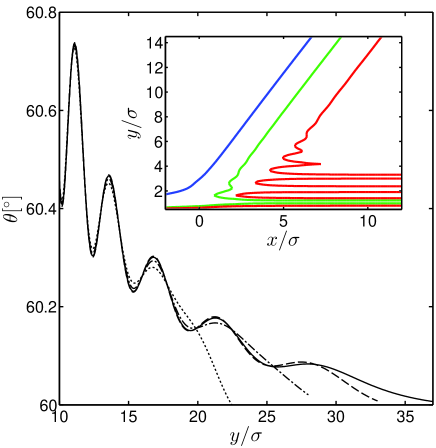
Figure 4: Slope of the isodensity line for $n=\left(n_{\text{vap}}+n_{\text{liq}}\right)/2$ for $y_{\text{max}}=\{20,25,30,35\}$, represented by the dotted, dash-dotted, dashed and solid lines, respectively. Computations are done on a grid with $\theta_{\text{n}}=60^{\circ}$. The substrate strength is $\alpha_{\text{w}}\sigma^{3}/\varepsilon=1.25$, such that $\theta_{Y}=60.0^{\circ}$. The inset depicts a contour plot of the contact line region. The contour lines correspond to number densities $(n-n_{\text{vap}})/(n_{\text{liq}}-n_{\text{vap}})=\{0.05,0.5,0.95\}$ from left to right, respectively.

We note that to solve the Euler-Lagrange Eq. (2), it is necessary to compute the functional derivative of $\mathcal{F}_{\text{attr}}[n]$. This corresponds to a convolution of the density profile $n({\bf r})$ with the attractive interaction potential $\phi_{\text{attr}}\left(|{\bf r}|\right)$, given by

$$\frac{\delta\mathcal{F}_{\text{attr}}[n]}{\delta n\left({\bf r}\right)} =\int\phi_{\text{attr}}({|{\bf r}-{\bf r}^{\prime}|})n({\bf r}^{\prime})\text{d}{\bf r}^{\prime}.$$ (17)

Let us describe briefly how this expression is computed numerically at a collocation point ${\bf r}$. It is worth noting that $\phi_{\text{attr}}(r)$ vanishes for $r\leq\sigma$. Hence, for each point ${\bf r}=(x,y)$, an area given by $\mathcal{A}_{\bf r}=\{{\bf r}^{\prime}=(x^{\prime},y^{\prime})\in\mathbb{R}^{2}|y^{\prime}>0,|{\bf r}^{\prime}-{\bf r}|>\sigma\}$ is discretized. Depending on the value of $y$, $\mathcal{A}_{\bf r}$ is divided into two or three subareas which are discretized separately using spectral collocation methods. We emphasize that technically, by employing a spectral method and placing collocations on the full area $\mathcal{A}_{\bf r}$, we do not introduce a cutoff for $\phi_{\text{attr}}$. This is particularly convenient for our choice of long-range fluid-fluid interactions. The numerical accuracy is instead limited by the quality of the maps used to discretize $\mathcal{A}_{\bf r}$ - including the choice of mapping parameters, number of collocation points, and the quality of the discretization of $n({\bf r})$ on the original grid. After interpolating the values of the density onto the collocation points of $\mathcal{A}_{\bf r}$, the density is multiplied with $\phi_{\text{attr}}$ such as given in (17) and the integration is performed on $\mathcal{A}_{\bf r}$. The procedure is repeated for each collocation point. The result of the interpolation and subsequent multiplication and integration is assembled in a convolution matrix in a preprocessing step.

All computations were performed using Matlab on a Intel Core i7-3770, 3.4GHz desktop PC with 8GB RAM running Windows 7. Preprocessing the FMT integration matrices and the convolution matrices for a grid with a specific $\theta_{\text{n}}$ with $50\times 80$ collocation points takes approximately 3.5h. Solving the Euler-Lagrange Eq. (2) for a specific $y_{\max}$ takes 0.5h–2h depending on the specific configuration.

IV Hamiltonian approaches and disjoining pressure

Computations for full macroscopic systems such as macroscopic droplets require a coarse-grained approach. One way to retain essential information of the structure of the contact line without computing the full density profile is through interface Hamiltonian approaches which reduce the dimension by one.Lipowsky and Fisher (1987); Mikheev and Weeks (1991) In particular, for systems which are not too close to the critical point, the film height profile of the liquid-vapor interface $h(x)$ can be studied by minimizing the Hamiltonian Herring and Henderson (2010)

$$H[h]=\int_{-\infty}^{\infty}\left\{\gamma_{\text{lv}}\left(\sqrt{1+(h^{\prime})^{2}}-1\right)+V(h)\right\}\text{d}x,$$ (18)

where $h^{\prime}={\text{d}h}/{\text{d}x}$ is the slope of the interface and $V(h)$ is the effective interface potential. Minimising the Hamiltonian with respect to $h(x)$ leads to the defining equation for the height profile

$$-\Pi(h(x))=\gamma_{\text{lv}}\frac{\text{d}}{\text{d}x}\left(\frac{h^{\prime}(x)}{\sqrt{1+\left(h^{\prime}(x)\right)^{2}}}\right),$$ (19)

where the disjoining pressure is the negative derivative of the interface potential

$$\Pi\left(h\right){\mathrel{\mathop{:}}=}-\frac{\text{d}V}{\text{d}h}.$$ (20)

Integrating Eq. (19) along the coordinate parallel to the wall leads to

$$-\int_{-\infty}^{x}\Pi(\hat{x})\text{d}\hat{x} =\gamma_{\text{lv}}\left(\frac{h^{\prime}}{\sqrt{1+(h^{\prime})^{2}}}\right)$$

$$=\gamma_{\text{lv}}\sin\theta(x),$$ (21)

where it was used that the film converges to a constant wall-vapor film with film height $\lim_{x\to-\infty}h(x)=h_{0}$. For $x\to\infty$, this corresponds with the sum rule representing the normal force balance from Young’s equation Derjaguin and Churaev (1986)

$$-\int_{-\infty}^{\infty}\Pi(h(x))\text{d}x=\gamma_{\text{lv}}\sin\theta_{\text{Y}},$$ (22)

where it was used that the film converges to a wedge with the Young contact angle $\lim_{x\to\infty}h^{\prime}(x)=\tan\theta_{\text{Y}}$. Similarly, integrating (19) with respect to the film height $h$ gives

$$\int_{h_{0}}^{h(x)}\Pi(\hat{h})\text{d}\hat{h} =\gamma_{\text{lv}}\left[\frac{1}{\sqrt{1+\left(h^{\prime}(\hat{x})\right)^{2}}}\right]_{\hat{x}=-\infty}^{\hat{x}=x}$$

$$=\gamma_{\text{lv}}\left(\cos\theta(x)-1\right).$$ (23)

Integrating up to $h=\infty$ yields the important expression from Derjaguin-Frumkin theory Derjaguin and Churaev (1986)

$$-\int_{h_{0}}^{\infty}\Pi\left(h\right)\text{d}h=\gamma_{\text{lv}}\left(1-\cos\theta_{\text{Y}}\right).$$ (24)

We note that the sum rules (22) and (24) hold independently of the exact definition of the interface potential.

An accurate model for the interface potential $V$ is crucial in order to retain important information about the structure of the contact line. Usually, $V(h)$ is defined as the interface potential for a planar film of height $h$.Bonn et al. (2009) In the last decade, Hamiltonian models have been suggested which take into account nonlocal effects due to changes of the height profile along the substrate. These include nonlocal models for short-ranged wetting,Parry et al. (2006) as well as models which include the slope of the height profile in the interface potential.Dai, Leal, and Redondo (2008) We now compare one local model of the disjoining pressure with a model based on a full DFT computation of a liquid wedge and test their predictive capabilities.

IV.1 Adsorption isotherm

For a planar liquid film and under the assumption that the free energy is a function of the film thickness only,Derjaguin and Churaev (1986); Frumkin (1938) the grand potential per unit area can be reduced to

$$\gamma\left(\ell,\mu\right)=f(\ell)-\mu\ell\Delta n,$$ (25)

where $\Delta n=n_{\text{liq}}-n_{\text{vap}}$. We note that Eq. (25) can be derived from the general formulation of the grand potential (1) by assuming a dependence of the density profile $n(y)$ on the film thickness $\ell$ but without any dependence on the chemical potential. One method to do this is through a simple sharp-interface approximation. $f(\ell)$ is then the reduced form of the part $\mathcal{F}[n]+\int n({\bf r})V_{\text{ext}}({\bf r})\text{d}{\bf r}$ in Eq. (1). At equilibrium, $\ell$ minimizes $\gamma$. Let us define $\mu_{\text{eq}}(\ell)$ as the chemical potential at which a film of thickness $\ell$ is at equilibrium

$$\mu_{\text{eq}}(\ell){\mathrel{\mathop{:}}=}\frac{1}{\Delta n}\frac{\text{d}f}{\text{d}\ell}.$$ (26)

In the planar case, $\gamma$ corresponds to the effective interface potential $V(h)$, and following Frumkin’s derivation,Frumkin (1938) the disjoining pressure is defined by the negative derivative of this quantity with respect to film thickness, leading to

$$\Pi_{\text{I}}\left(\ell,\mu\right){\mathrel{\mathop{:}}=}-\frac{\partial\gamma}{\partial\ell}=\left(\mu-\mu_{\text{eq}}\left(\ell\right)\right)\Delta n,$$ (27)

linking the disjoining pressure with the adsorption isotherm.Henderson (2005) We note that by definition the disjoining pressure is zero for the equilibrium film thickness, consistent with $\mu$. In other words, the disjoining pressure gives the excess pressure acting on the substrate for liquid films which are perturbed or off-equilibrium, e.g. through fluctuations or because of forcing through boundary conditions.

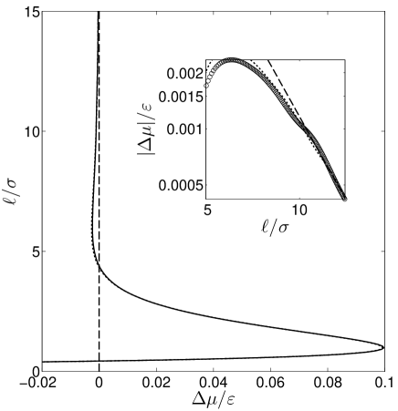
Figure 5: Adsorption isotherm for $\alpha_{\text{w}}\sigma^{3}/\varepsilon=1.375$ ($\theta_{\text{Y}}=41.1^{\circ}$). The solid line represents the film thickness (30) of equilibrium density distributions, and the dotted line represents the modified sum rule (32). The contact angle obtained from sum rule (24) is $41.1^{\circ}$, in excellent agreement with the Young contact angle $\theta_{\text{Y}}$. The inset shows the asymptotic behavior for $\ell\to\infty$, as $\Delta\mu\sim\ell^{-3}$. The dashed line is a fit for $\ell\in[10\sigma,15\sigma]$, giving $\Delta\mu=a\ell^{-3}$ with the coefficient $a=-1.16\varepsilon\sigma^{3}$. The circles in the inset represent the individual DFT computations of the equilibrium density, which in the main plot are connected by the solid line for convenience.

IV.2 Normal force balance

Dzyaloshinskii, Lifshitz and Pitaevskii (DLP) employed quantum-field theory to directly compute the force acting on the surface due to an adsorbed film, and related it to the disjoining pressure.Dzyaloshinskii, Lifshitz, and Pitaevskii (1961) In other words, DLP related the chemical potential difference (27) to the excess pressure on the substrate wall due to an adsorbed liquid film. For a discussion of this connection, see also Ref. Henderson, 2011a. In particular, the force acting on the substrate at saturation chemical potential $\mu_{\text{sat}}$ for a density profile $n_{\ell}$ is given by Mikheev and Weeks (1991); Henderson (2005)

$$\Pi(\ell)=-\int_{-\infty}^{\infty}\left(n_{\ell}(y)-n_{\ell=\infty}(y)\right)V_{\text{ext}}^{\prime}(y)\text{d}y,$$ (28)

where $n_{\ell}(y)$ is a density profile at chemical potential $\mu_{\text{sat}}$ but with the additional constraint of film thickness $\ell$. Such profiles may be either partially stable or unstable, and are obtained by minimizing the excess grand potential subject to the constraint of fixed adsorption. Henderson (2005) $n_{\ell=\infty}(y)$ is thus the density profile of the equilibrium case of a film of infinite thickness accounting for the contribution from the bulk pressure as Henderson (1992)

$$p_{\text{sat}}=-\int_{-\infty}^{\infty}n_{\ell=\infty}(y)V_{\text{ext}}^{\prime}(y)\text{d}y.$$ (29)

We note that in Eq. (28), the disjoining pressure would decay exponentially if both the fluid-fluid and the fluid-substrate interactions were short-range. Here, however, the long-range fluid-substrate interactions lead to an algebraic decay of the disjoining pressure. Furthermore, the interplay between long-range fluid-fluid and the short-range part of the fluid-substrate interactions also lead to an algebraic contribution to the disjoining pressure with an identical power series in terms of film thickness $\ell$.Henderson (2005) This means that one cannot apply asymptotic theory to derive a distinct representation for long-range and short-range interactions.Henderson (2005) While DLP circumvent this problem by only applying their theory to films of mesoscopic scales,Dzyaloshinskii, Lifshitz, and Pitaevskii (1961) we will instead use the full numerical solution of the disjoining pressure in order to define a height profile through the three-phase contact line.

V Results and discussion

In Fig. 5, we compare the Derjaguin-Frumkin route of the disjoining pressure (27) and the definition from the normal force balance for a planar film on a solid substrate. We have employed a numerical continuation scheme to compute the full bifurcation diagram for the adsorption isotherm including its meta- and unstable branches. As an order parameter for the number density distribution, we have used the adsorption film thickness:

$$\ell{\mathrel{\mathop{:}}=}\frac{1}{\Delta n}\int_{0}^{\infty}\left(n(y)-n_{\text{vap}}\right)\text{d}y,$$ (30)

where the vapor density $n_{\text{vap}}$ is taken at the chemical potential at which $n(y)$ is in equilibrium. In the large film thickness limit, dispersion forces enforce an algebraic approach of the saturation line Dietrich (1988) as

$$\Delta\mu\sim\ell^{-3}\qquad\text{for}\quad\ell\to\infty,$$ (31)

where $\Delta\mu=\mu-\mu_{\text{sat}}$ is the deviation of the chemical potential from its saturation value. Note that the density profiles obtained when solving for the adsorption isotherm are not computed at saturation chemical potential, and can therefore not be used as $n_{\ell}$ in Eq. (28). To allow for a comparison of the two routes to the disjoining pressure, we have instead combined Eqs. (28) and (29) to define a generalized form of sum rule (28):

$$\Pi[n]=-\int_{-\infty}^{\infty}n(y)V_{\text{ext}}^{\prime}(y)\text{d}y-p_{\infty},$$ (32)

where $p_{\infty}$ is the bulk pressure of the given density profile $n$ as $y\to\infty$. The computations depicted in Fig. 5 give an excellent agreement between the two definitions.

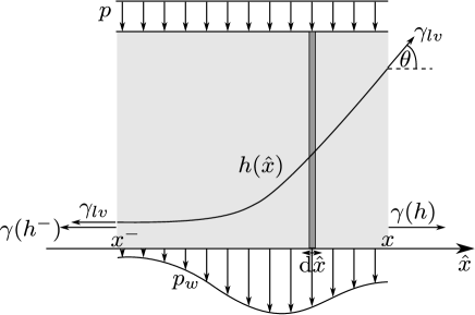
Figure 6: Sketch of a mechanical model which describes the normal and the parallel force balances (21) and (23) for an adsorbed liquid film in the box $[x^{-},x]\times[0,\infty]$, where $x^{-}\to-\infty$. The force acting from the external potential modeling the substrate on the fluid strip $[\hat{x},\hat{x}+\text{d}\hat{x}]\times[0,\infty]$ corresponds to the disjoining pressure $\Pi=p_{w}-p$ times the length of the interval $\text{d}\hat{x}$. Here, $p_{w}\text{d}\hat{x}=-\text{d}\hat{x}\int_{-\infty}^{\infty}n(\hat{x},y)V_{\text{ext}}^{\prime}(y)\text{d}y$ is the net force acting from the substrate on the fluid strip. The liquid-vapor surface tension $\gamma_{\text{lv}}$ accounts for fluid-fluid interactions. The forces accounting for the fluid-fluid interactions stemming from the distortion of the density profile due to the substrate are included as a wall-liquid film-vapor potential $\gamma(h)$, acting at the wall.

Let us now consider if there is a similar equivalence of disjoining pressure definitions for the case of varying height profiles $h(x)$. For this purpose, consider Eqs. (21) and (23). We can formulate a mechanical model for the contact line with height profile $h(x)$, in which Eq. (21) is a momentum balance in the direction normal to the wall, and Eq. (23) is a momentum balance parallel to the wall for a system $(\hat{x},\hat{y})\in[-\infty,x]\times[0,\infty]$ (see Fig. 6). Analogously, Eq. (19) represents the Young-Laplace equation modeling the pressure jump across a curved interface in which the disjoining pressure acts as a gauge pressure in the liquid film. The fact that the disjoining pressure in Eq. (21) represents the force of the substrate acting on the fluid film allows the generalisation of Eq. (28) to two dimensions by Herring and Henderson (2010); Henderson (2011a)

$$\Pi_{\text{II}}\left(x\right){\mathrel{\mathop{:}}=}-\int_{-\infty}^{\infty}\left(n(x,y)-n(\infty,y)\right)V_{\text{ext}}^{\prime}(y)\text{d}y,$$ (33)

where it was used that $n(x,y)V_{\text{ext}}^{\prime}(y)$ is the force acting through the external potential on the fluid element at point $(x,y)$, and where the pressure acting from the bulk vapor was subtracted using Eq. (29).

The definitions (27) and (33) of disjoining pressures $\Pi_{\text{I}}(h)$ and $\Pi_{\text{II}}(x)$, respectively, allow in turn for the definition of two alternative height profiles $h_{\text{I}}$ and $h_{\text{II}}$. Integrating (23) leads to the definition of the film height profile through the ordinary differential equation

$$h_{\text{I}}^{\prime}=\tan\left\{{\cos^{-1}\left(1+\frac{1}{\gamma_{\text{lv}}}\int_{h_{0}}^{h_{\text{I}}}\Pi_{\text{I}}(\hat{h})\text{d}\hat{h}\right)}\right\},$$ (34)

with boundary condition

$$h_{\text{I}}\left(x_{B}\right)=h_{B},$$ (35)

for some $x_{B},h_{B}$. Let us note that $h_{\text{I}}$ is translationally invariant through the boundary condition. Integrating Eq. (21) leads to the height profile

$$h_{\text{II}}^{\prime}(x)=-\tan\left\{\sin^{-1}\left(\frac{1}{\gamma_{\text{lv}}}\int_{-\infty}^{x}\Pi_{\text{II}}(\hat{x})\text{d}\hat{x}\right)\right\},$$ (36)

with boundary condition

$$h_{\text{II}}(-\infty)=h_{0},$$ (37)

where $h_{0}$ is the (equilibrium) height of the vapor film. Note that while $h_{\text{I}}$ is translationally invariant through boundary condition (35), $h_{\text{II}}$ is only invariant up to an additive constant, which does not change the position of the contact line in the direction parallel to the wall. Finally, we compare the film height profiles $h_{\text{I}}$ and $h_{\text{II}}$ with the adsorption film thickness

$$h_{\text{III}}(x)=\frac{1}{\Delta n}\int_{0}^{\infty}\left(n(x,y)-n_{\text{vap}}\right)\text{d}y.$$ (38)

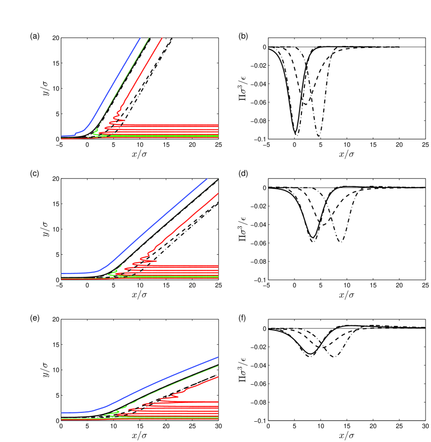
Figure 7: Density contours (left column, figures (a),(c),(e)) and disjoining pressures (right column, figures (b), (d), (f)) for three contact line regions. The top, middle and bottom rows depict results for the three different substrate strengths $\alpha_{\text{w}}\sigma^{3}/\varepsilon=\{1.25,1.375,1.47\}$, corresponding to Young contact angles $60.0^{\circ}$, $41.1^{\circ}$ and $20.4^{\circ}$, respectively. In the left column, the contour lines correspond to number densities $\left(n-n_{\text{vap}}\right)/\left(n_{\text{liq}}-n_{\text{vap}}\right)=\{0.05,0.5,0.95\}$ from left to right, respectively. Height profiles $h_{\text{II}}$ and $h_{\text{III}}$ as in (36) and (38) are represented by the dashed and solid lines, respectively. $h_{\text{I}}$ as defined by (34) is plotted with dash-dotted lines twice, to match $h_{\text{II}}$ and $h_{\text{III}}$ for large film thicknesses, through a corresponding choice of $h_{B}$ in (35). We note that in the left column, the solid, one of the dash-dotted lines and the density isoline representing $\left(n-n_{\text{vap}}\right)/\left(n_{\text{liq}}-n_{\text{vap}}\right)=0.5$ are virtually indistinguishable. The right column depicts the disjoining pressure profiles. The dashed line represents $\Pi_{\text{II}}\left(x\right)$ as defined in Eq. (33), the dash-dotted line represents $\Pi_{\text{I}}\left(h_{\text{I}}(x)\right)$ for the two shifted cases $h_{\text{I}}$ as depicted in the left column, and employing data of the adsorption isotherm for the disjoining pressure, using (27). For comparison with Eq. (19), the scaled curvature $-\gamma_{\text{lv}}\text{d}\left(h_{\text{III}}^{\prime}/\sqrt{1+(h_{\text{III}}^{\prime})^{2}}\right)/\text{d}x$ is plotted with the solid line.

In Fig. 7, we show results of the equilibrium DFT-FMT computations in the contact line region for three different substrate strengths, together with plots of the height profiles $h_{\text{I}}$, $h_{\text{II}}$ and $h_{\text{III}}$ and the disjoining pressure profiles $\Pi_{\text{I}}$ and $\Pi_{\text{II}}$. We note that we have plotted $h_{\text{I}}$ twice, to match $h_{\text{II}}$ and $h_{\text{III}}$ for large film thicknesses, by use of the corresponding boundary condition (35). It is also worth noting that through Eq. (19), the disjoining pressures correspond to the scaled curvatures of the height profiles. In all cases, the numerical results show an excellent agreement of sum rules (24) and (22). This is shown in Table 1, where we compare the contact angles obtained by evaluating sum rules (24) and (22) through the limiting behavior $\lim_{x\to\infty}h_{\text{I/II}}(x)$, with the Young contact angle $\theta_{\text{Y}}$. For ease of comparison, let us define

$$\theta_{\text{Y,I/II}}=\lim_{x\to\infty}\tan^{-1}\left(h^{\prime}_{\text{I/II}}(x)\right).$$ (39)

We note that, as the height profiles $h_{\text{I,II}}$ are defined through Eq. (19), the sum rules (22) and (24) lead to the same limiting contact angles for each of the height profiles.

$\alpha_{\text{w}}\sigma^{3}/\varepsilon$	$\theta_{\text{Y}}$	$\theta_{\text{Y,I}}$	$\theta_{\text{Y,II}}$
$1.25$	$60.0^{\circ}$	$60.0^{\circ}$	$59.1^{\circ}\pm 1.7^{\circ}$
$1.375$	$41.1^{\circ}$	$41.1^{\circ}$	$39.9^{\circ}\pm 2^{\circ}$
$1.47$	$20.4^{\circ}$	$20.4^{\circ}$	$22.1^{\circ}\pm 2^{\circ}$

Table 1: The Young contact angle $\theta_{\text{Y}}$ in Eq. (16) is compared with the contact angles obtained from the limiting behavior of the slope of the height profiles $h^{\prime}_{\text{I/II}}$, defined in Eq. (39) for substrates of different strengths $\alpha_{\text{w}}$. As the height profiles are defined through Eqs. (34) and (36), respectively, this amounts to an error-check of sum rules (24) and (22), respectively. Note that both height profiles $h_{\text{I/II}}$ satisfy Eq. (19), which means that both sum rules (24) and (22) lead to the same limiting contact angle for each of the height profiles. Error bounds for $\theta_{\text{Y,II}}$ were estimated employing the numerical error in the computation of $\Pi_{\text{II}}(\pm\infty)$.

The density profiles in Figs. 4 and 7 reveal the structure of the fluid in the immediate vicinity of the contact line. It is evident that the fluid particles are densely packed close to the wall at the wall-liquid interface due to hard-sphere effects. In particular, the transition between the wall-vapor interface and the wall-liquid interface seems to lead to a quasi step-like increase of the density. This influences the structure of the liquid-vapor interface in the vicinity of the contact line. As attraction with the wall increases and the contact angle decreases, packing close to the wall becomes even more pronounced. Most importantly, we observe how the structure of the liquid-vapor interface is significantly perturbed close to the wall due to hard-sphere packing effects and ultimately merges with the wall-vapor interface ahead of the macroscopic liquid wedge. Finally, we see that for $y>5\sigma$, the film height based on the adsorption, $h_{\text{III}}$, seems to coincide for all three cases with the isodensity line for $\left(n-n_{\text{vap}}\right)/\left(n_{\text{liq}}-n_{\text{vap}}\right)=0.5$.

Let us now look at the results for the film heights $h_{\text{I}}$ and $h_{\text{II}}$. We can make two main observations. First, there seems to be a reasonable agreement between height profiles $h_{\text{I}}$ and $h_{\text{III}}$ in Figs. 7 (a), (c) and (e). A more accurate means to compare the behavior of the height profiles is through their corresponding disjoining pressure profiles in Figs. 7 (b), (d) and (f). Note that the corresponding disjoining pressure plots correspond to the rescaled curvatures of the height profiles, in accordance with Eq. (19). We observe that the maximal curvature of both height profiles $h_{\text{I}}$ and $h_{\text{III}}$ agree very well. Also, the curvature of both height profiles $h_{\text{I}}$ and $h_{\text{III}}$ changes sign, which is more evident in Fig. 7 (f). In contrast, $h_{\text{II}}$ exhibits a lower curvature than $h_{\text{I}}$ and $h_{\text{III}}$ and it does not change its sign. Furthermore, $h_{\text{II}}$ approaches an isodensity line for $\left(n-n_{\text{vap}}\right)/\left(n_{\text{liq}}-n_{\text{vap}}\right)$ around $0.95$, i.e. much greater than $0.5$. We note that the results for $h_{\text{II}}$ are similar to results obtained in Ref. Herring and Henderson, 2010 for fluids with short-ranged interactions and using MC computations in that the height profile $h_{\text{II}}$ approaches isodensity lines $\left(n-n_{\text{vap}}\right)/\left(n_{\text{liq}}-n_{\text{vap}}\right)\approx 0.95$ for large $x$.

At the same time the results are surprising for two reasons. First, the height profile $h_{\text{I}}$ is defined through the disjoining pressure $\Pi_{\text{I}}$, which is based on computations of planar wall-fluid interfaces. Hence, it loses some of the physics associated with the true 2D contact line region profiles in that it does not include any nonlocal effects in the direction parallel to the substrate, or effects due to the slope of the liquid-vapor interface. Nevertheless, it does give a good prediction of the adsorption height profile $h_{\text{III}}$ for contact angles up to $60^{\circ}$. Second, the height profile $h_{\text{II}}$, which is based on the disjoining pressure $\Pi_{\text{II}}$, seems to behave very differently in the vicinity of the contact line compared to the DFT-FMT computations, even though it contains information from the full 2D density distribution.

The computations of height profiles through a three-phase contact line bring us a considerable step closer to addressing one of the main questions posed in the discussion papers that appeared in Eur. Phys. J.: Spec. Top., special issue ‘Wetting and Spreading Science - quo vadis?’, MacDowell (2011a); Henderson (2011a); MacDowell (2011b); Henderson (2011b, c) which is: Considering the disjoining pressure based on the normal force balance $\Pi_{\text{II}}(x)$, which is the correct choice of order parameter $\ell$, if indeed there is one, that gives an accurate local function $\Pi_{\text{II}}(\ell)$? In this special issue, Henderson Herring and Henderson (2010); Henderson (2011b) noted that the disjoining pressure is inherently non-local, and that there is no unique pair $\left(\Pi,\ell\right)$, in accordance with Parry et al. Parry et al. (2006) In this context, MacDowell MacDowell (2011b) notes that the nonlocality of the disjoining pressure can only matter very close to the contact line, as far enough from the contact line Young’s equation must be satisfied.

The computations presented in this study are a decisive first step towards addressing the question of universality of the disjoining pressures $\Pi_{\text{I}}$ and $\Pi_{\text{II}}$. In particular, we show that for the cases considered here, the disjoining pressure obtained from the adsorption isotherm seems to accurately predict the height profile even very close to the contact line. However, we also note that the disjoining pressure based on the adsorption isotherm apparently does not correspond to the excess pressure acting on the substrate obtained from a normal force balance. One way to test if there is a unique pair $\left(\Pi,\ell\right)$ would be by comparing static nanodroplets with each of the two disjoining pressures and compare the results to those obtained from DFT-FMT, but this is beyond the scope of the present study.

VI Conclusion

We have computed the density distribution in the vicinity of a three-phase contact line at equilibrium using a DFT-FMT theory with a mean-field Barker-Henderson approach for long-range particle interactions for three different substrate strengths, corresponding to contact angles of $20.4^{\circ}$, $41.1^{\circ}$ and $60.0^{\circ}$. We have confirmed that the results satisfy basic sum rules to a good accuracy. The computations allow us to probe the fluid structure in the immediate vicinity of the contact line: Fluid particles are closely packed close to the contact line due to hard-sphere effects. This packing leads to a quasi-stepwise increase of the density as the wall is approached. For smaller contact angles, i.e. as the attraction of the wall increases, the stepwise structure of the density is amplified.

Furthermore, we have employed numerical results of adsorption isotherms for different substrate strengths to define a disjoining pressure in the spirit of Derjaguin-Frumkin adsorption theory. We have also used the results from our equilibrium DFT computations of the density profile to define a disjoining pressure based on the normal force balance at the contact line. Via an effective mean-field Hamiltonian approach, both disjoining pressures were employed to define height profiles to describe the three-phase contact line. These were compared with the height profile defined by the adsorption of the equilibrium density obtained from DFT.

The results of the comparison of the two disjoining pressures can be summarized as follows: The disjoining pressure based on the adsorption isotherm following the Derjaguin-Frumkin theory shows good agreement with the DFT adsorption height profile in terms of maximal curvature and behavior for large film heights. In contrast, the height profile defined through the disjoining pressure based on a normal-force balance shows a very different behavior, in particular, its maximal curvature is lower than that obtained from DFT and Derjaguin-Frumkin, and it shows a different behavior for large film heights compared to the other height profiles. Our results hence show that the disjoining pressure definition which gives the better prediction for the adsorption film thickness is based on the adsorption isotherm and does not correspond to the excess pressure acting on the substrate, thus contradicting the classical notion of what the disjoining pressure stands for.

One important restriction of the model used in this work is that it is of a mean-field type which does not take into consideration thermal fluctuations. Archer and Evans (2013); Evans et al. (1993); MacDowell et al. (2014) While we do not expect this to alter the general results of this work, fluctuations cannot be neglected generally. For example, fluctuations were observed when modeling a contact line using an MC algorithm for a fluid with short-range fluid-fluid interactions. Herring and Henderson (2010) We note that including fluctuations in the fluid description calls for an amended Hamiltonian theory, in which the liquid-vapor interface has to be assumed to depend on the film thickness, such as suggested by MacDowell et al. for long-range fluid-fluid interactions. MacDowell et al. (2014) However, incorporating fluctuations in a DFT model is highly nontrivial Archer and Evans (2013) and beyond the scope of this work.

Clearly, there are many future directions that can be explored. For instance, how chemically and/or topographically heterogeneous substrates, which are known to influence wetting characteristics substantially, Savva and Kalliadasis (2009); Savva, Kalliadasis, and Pavliotis (2010); Savva, Pavliotis, and Kalliadasis (2011a, b); Vellingiri, Savva, and Kalliadasis (2011) affect the fluid structure in the vicinity of the contact line. Of particular interest would also be the much more involved dynamic case. For this purpose, the dynamic DFT approach developed recently for colloidal fluids Goddard, Pavliotis, and Kalliadasis (2012); Goddard et al. (2012, 2013); Goddard, Nold, and Kalliadasis (2013) should serve as a basis for the accurate modeling of moving contact lines as it takes into account both microscale inertia and hydrodynamic interactions, two effects which strongly influence nonequilibrium properties. We shall address these and related issues in future studies.

VII Acknowledgments

We acknowledge financial support from ERC Advanced Grant No. 247031 and Imperial College through a DTG International Studentship.

References

- Seemann et al. (2005) R. Seemann, M. Brinkmann, E. J. Kramer, F. F. Lange, and R. Lipowsky, “Wetting morphologies at microstructured surfaces,” Proc. Natl. Acad. Sci. U.S.A. 102, 1848–1852 (2005).
- Rauscher and Dietrich (2008) M. Rauscher and S. Dietrich, “Wetting phenomena in nanofluidics,” Annu. Rev. Mater. Res. 38, 143–172 (2008).
- Jensen and Grotberg (1992) O. E. Jensen and J. B. Grotberg, “Insoluble surfactant spreading on a thin viscous film: shock evolution and film rupture,” J. Fluid Mech. 240, 259–288 (1992).
- Wong, Fatt, and Radke (1996) H. Wong, I. Fatt, and C. J. Radke, “Deposition and thinning of the human tear film,” J. Colloid Interface Sci. 184, 44–51 (1996).
- MacDowell (2011a) L. G. MacDowell, “Computer simulation of interface potentials: Towards a first principle description of complex interfaces?” Eur. Phys. J. Special Topics 197, 131–145 (2011a).
- Herring and Henderson (2010) A. R. Herring and J. R. Henderson, “Simulation study of the disjoining pressure profile through a three-phase contact line,” J. Chem. Phys. 132, 084702 (2010).
- Das and Binder (2010) S. K. Das and K. Binder, “Does Young’s equation hold on the nanoscale? A Monte Carlo test for the binary Lennard-Jones fluid,” Europhys. Lett. 92, 26006 (2010).
- Werder et al. (2001) T. Werder, J. H. Walther, R. L. Jaffe, T. Halicioglu, F. Noca, and P. Koumoutsakos, “Molecular dynamics simulation of contact angles of water droplets in carbon nanotubes,” Nano Lett. 1, 697–702 (2001).
- Tretyakov et al. (2013) N. Tretyakov, M. Müller, D. Todorova, and U. Thiele, “Parameter passing between molecular dynamics and continuum models for droplets on solid substrates: The static case,” J. Chem. Phys. 138, 064905 (2013).
- Evans (1979) R. Evans, “The nature of the liquid-vapour interface and other topics in the statistical mechanics of non-uniform, classical fluids,” Adv. Phys. 28, 143–200 (1979).
- Wu (2006) J. Wu, “Density functional theory for chemical engineering: From capillarity to soft materials,” AIChE J. 52, 1169–1193 (2006).
- Stewart and Evans (2005) M. C. Stewart and R. Evans, “Wetting and drying at a curved substrate: Long-ranged forces,” Phys. Rev. E 71, 011602 (2005).
- Nold, Malijevský, and Kalliadasis (2011) A. Nold, A. Malijevský, and S. Kalliadasis, “Wetting on a spherical wall: Influence of liquid-gas interfacial properties,” Phys. Rev. E 84, 021603 (2011).
- Berim and Ruckenstein (2008) G. O. Berim and E. Ruckenstein, “Nanodrop on a nanorough solid surface: Density functional theory considerations,” J. Chem. Phys. 129, 014708 (2008).
- Ruckenstein and Berim (2010) E. Ruckenstein and G. O. Berim, “Microscopic description of a drop on a solid surface,” Adv. Colloid Interface Sci. 157, 1–33 (2010).
- Malijevský and Parry (2013) A. Malijevský and A. O. Parry, “Critical point wedge filling,” Phys. Rev. Lett. 110, 166101 (2013).
- Yatsyshin, Savva, and Kalliadasis (2013) P. Yatsyshin, N. Savva, and S. Kalliadasis, “Geometry-induced phase transition in fluids: Capillary prewetting,” Phys. Rev. E 87, 020402(R) (2013).
- Zhou, Mi, and Zhong (2012) D. Zhou, J. Mi, and C. Zhong, “Three-dimensional density functional study of heterogeneous nucleation of droplets on solid surfaces,” J. Phys. Chem. B 116, 14100–14106 (2012).
- Bonn et al. (2009) D. Bonn, J. Eggers, J. Indekeu, J. Meunier, and E. Rolley, “Wetting and spreading,” Rev. Mod. Phys. 81, 739–805 (2009).
- Béguin et al. (2013) L. Béguin, A. Vernier, R. Chicireanu, T. Lahaye, and A. Browaeys, “Direct Measurement of the van der Waals Interaction between Two Rydberg Atoms,” Phys. Rev. Lett. 110, 263201 (2013).
- Henderson (2005) J. R. Henderson, “Statistical mechanics of the disjoining pressure of a planar film,” Phys. Rev. E 72, 051602 (2005).
- Dietrich (1988) S. Dietrich, “Wetting phenomena,” in Phase Transitions and Critical Phenomena, Vol. 12, edited by C. Domb and J. L. Lebowitz (Academic Press, London, 1988) Chap. 1, p. 2.
- Bauer and Dietrich (1999) C. Bauer and S. Dietrich, “Wetting films on chemically heterogeneous substrates,” Phys. Rev. E 60, 6919–6941 (1999).
- Hofmann et al. (2010) T. Hofmann, M. Tasinkevych, A. Checco, E. Dobisz, S. Dietrich, and B. M. Ocko, “Wetting of nanopatterned grooved surfaces,” Phys. Rev. Lett. 104, 106102 (2010).
- Pereira and Kalliadasis (2012) A. Pereira and S. Kalliadasis, “Equilibrium gas-liquid-solid contact angle from density-functional theory,” J. Fluid Mech. 692, 53–77 (2012).
- Roth (2010) R. Roth, “Fundamental measure theory for hard-sphere mixtures: a review,” J. Phys.: Condens. Matter 22, 063102 (2010).
- Merath (2008) R.-J. C. Merath, Microscopic calculation of line tensions, Ph.D. thesis, Universität Stuttgart (2008).
- Lipowsky and Fisher (1987) R. Lipowsky and M. E. Fisher, “Scaling regimes and functional renormalization for wetting transitions,” Phys. Rev. B 36, 2126–2141 (1987).
- Mikheev and Weeks (1991) L. V. Mikheev and J. D. Weeks, “Sum rules for interface Hamiltonians,” Physica A 177, 495–504 (1991).
- Derjaguin (1987) B. V. Derjaguin, “Some results from 50 years’ research on surface forces,” in Surface Forces and Surfactant Systems, Progress in Colloid & Polymer Science, Vol. 74 (Springer, Berlin-Heidelberg, 1987) pp. 17–30.
- Derjaguin and Churaev (1986) B. V. Derjaguin and N. V. Churaev, “Properties of water layers adjacent to interfaces,” in Fluid interfacial phenomena, edited by C. A. Croxton (Wiley, New York, 1986) pp. 663–738.
- Frumkin (1938) A. N. Frumkin, “Über die Erscheinungen der Benetzung und des Anhaftens von Bläschen. I,” Acta Physicochim. URSS 9, 313 (1938).
- Derjaguin and Obuchov (1936) B. V. Derjaguin and E. Obuchov, Acta Physicochim. URSS 5, 1 (1936).