How Nested Infection Networks in Host-Phage Communities Come To Be

Abstract.

We show that a chemostat community of bacteria and bacteriophage in which bacteria compete for a single nutrient and for which the bipartite infection network is perfectly nested is permanent, a.k.a. uniformly persistent, provided that bacteria that are superior competitors for nutrient devote the least to defence against infection and the virus that are the most efficient at infecting host have the smallest host range. This confirms earlier work of Jover et al [7] who raised the issue of whether nested infection networks are permanent. In addition, we provide sufficient conditions that a bacteria-phage community of arbitrary size with nested infection network can arise through a succession of permanent subcommunties each with a nested infection network by the successive addition of one new population.

Daniel A. Korytowski and Hal L. Smith

School of Mathematical and Statistical Sciences

Arizona State University

Tempe, AZ 85287, USA

1. introduction

This work is inspired by the recent paper of Jover, Cortez, and Weitz [7]. Noting that empirical studies strongly suggest that the bipartite infection networks observed in bacteria and virus communities tend to have a nested structure characterized by a hierarchy among both host and virus strains which constrains which virus may infect which host, they identify key tradeoffs between competitive ability of the bacteria hosts and defence against infection and, on the part of virus, between virulence and transmissibility versus host range such that a nested infection network can be maintained. They find that “bacterial growth rate should decrease with increasing defence against infection” and that “the efficiency of viral infection should decrease with host range”. Their mathematical analysis of a Lotka-Volterra model incorporating the above mentioned tradeoffs strongly suggests that the perfectly nested community structure of $n$-host bacteria and $n$-virus is permanent, sometimes also called persistent, or uniformly persistent [6, 12, 15]. Indeed, they establish several necessary conditions for permanence: (1) a positive equilibrium for the system with all host and virus populations at positive density exists, and (2) every boundary equilibrium of the $2n$-dimensional ordinary differential equations, where one or more population from the nested structure is missing, is unstable to invasion by at least one of the missing populations. They also note that while equilibrium dynamics are rare for such systems, invasability of boundary equilibria can imply invasability of general boundary dynamics provided permanence holds according to results of Hofbauer and Sigmund [6]. However, permanence of a perfectly nested infection network is not established in [7]. The famous example of three-species competition described by May and Leonard [9] shows that the necessary conditions mentioned above are not sufficient for permanence.

Permanence of bacteriophage and bacteria in a chemostat has been established for mathematical models of very simple communities consisting of a single virus and one or two host bacteria in [13, 6].

A nested infection network of three bacterial strains and three virus strains has the structure described in the infection table below. An ‘x’ in the matrix means that the host below is infected by the virus on the left while a blank entry indicates no infection; for example, the second column of three x’s indicates that bacteria $H_{1}$ is infected by virus $V_{1},V_{2}$ and $V_{3}$. Host $H_{1}$ is the least resistant to infection while $H_{3}$ is the most resistant; virus $V_{1}$ specializes on a single host while $V_{3}$ is a generalist, infecting all host.

$V_{3}$	x	x	x
$V_{2}$	x	x
$V_{1}$	x
	$H_{1}$	$H_{2}$	$H_{3}$

This community may have evolved by the sequential addition of one new population following a mutational event or the selection of a rare variant. Below, going back in time, we list in order the communities from which the one above may have evolved from an ancestral community consisting of a single bacteria and a single virus on the right.

$V_{2}$ x x $V_{1}$ x $H_{1}$ $H_{2}$ $H_{3}$     $V_{2}$ x x $V_{1}$ x $H_{1}$ $H_{2}$     $V_{1}$ x $H_{1}$ $H_{2}$     $V_{1}$ x $H_{1}$

Other possible evolutionary trajectories starting from the ancestral pair at the bottom are highly unlikely. Obviously, a new virus cannot evolve without there being a susceptible host for it; however, a new bacterial strain resistent, or partially resistent, to some virus may evolve. Obviously, the three-host, three-virus network need not be the end of the evolutionary sequence. A fourth bacterial strain may evolve resistance to all three virus.

Just such a sequence of mutational or selection events is observed in chemostat experiments starting from a single bacteria population and a single virus population and leading to a nested infection network. Chao et al [2] describe such a scenario in their experimental observations of E. Coli and phage $T7$. A bacterial mutant resistant to the virus is observed to evolve first. Resistance is conferred by a mutation affecting a receptor on the host surface to which the virus binds. Subsequently, a viral mutant evolves which is able to infect both bacterial populations. Eventually, another bacterial mutant arises which is resistant to both virus. Similar evolutionary scenarios are noted in the review of Bohannan and Lenski [1]. Thus, a nested infection structure can evolve as an arms race between host and parasite.

Our goal in this paper is to show that a nested infection network consisting of $n$ bacterial host and $n$ lytic virus is permanent given the trade-offs identified in [7]. Recall that permanence means that there is a positive threshold, independent of positive initial conditions of all populations, which every bacteria and virus density ultimately exceeds.

However, we replace the Lotka-Volterra model used by Jover et al [7] by a chemostat-based model where bacterial populations compete for nutrient and virus populations compete for hosts as in [2, 6, 13, 17], although we ignore latency of virus infection. Aside from the additional realism of including competition for nutrient, our model avoids the non-generic bacterial dynamics of the Lotka-Volterra model which possesses an $n-1$-dimensional simplex of virus-free equilibria.

Chemostat-based models of microbial competition for a single nutrient are known to induce a ranking of competitive ability among the microbes determined by their break-even nutrient concentrations for growth, here denoted by $\lambda$ but often by $R^{*}$ in the ecological literature. The competitive exclusion principle applies: a single microbial population, the one with smallest $\lambda$, drives all others to extinction [16, 14] in the absence of virus. In our model of a nested infection network, this host can be infected by every virus strain and as the $\lambda$ value of host strains increases (i.e., it becomes less competitive for nutrient) it is subject to infection by fewer virus strains. Virus populations are ranked by their efficiency at infecting host. The most efficient strain specializes on the host with smallest $\lambda$ and as infection efficiency decreases host range increases so that the virus strain of rank $k$ infects the $k$ most competitive host strains.

Our permanence result is a dramatic example of predator-mediated coexistence. In the absence of phage, only a single bacterial strain can survive. However, the addition of an equal number of phage to our microbial community with infection efficiency versus host range tradeoff as noted above lead to the coexistence of all populations.

In fact, we will show that the $n$-bacteria, $n$-virus community can arise through a succession of permanent sub-communities just as described in the infection tables above for the case $n=3$, starting with an ancestral community of one susceptible bacterial host and one virus. This is important because it ensures that the intermediate communities are sufficiently stable so as to persist until a fortuitous mutational or colonization event allows further progression. Permanence is not a guarantee of long term persistence since environmental stochasticity may intervene to cause an extinction event, especially when a population is in a low part of its cycle. See Figure 1 below. However, our permanence result implies that should an extinction event occur, the resulting community is likely to be a permanent one and therefore recovery is possible.

We also show that time averages of species densities are asymptotic to appropriate equilibrium levels. Solutions of our chemostat-based model are highly oscillatory, apparently aperiodic, just as those observed for the Lotka-Volterra system of Jover et al [7]. See Figure 1.

Perhaps it is interesting to note that the mathematical justification used to establish our results is to exploit the evolutionary sequence noted in the infection tables above by way of the principle of mathematical induction, establishing permanence in a given sub-community in the successional sequence by appealing to the permanence hypothesis of its predecessor in the sequence.

The competitive exclusion principle is critical to our approach. We will show that two virus strains cannot share the same set of bacterial hosts (i.e. cannot have the same host range) since one of the virus will be more efficient at exploiting the host and drive the other to extinction. Similarly, two bacterial strains cannot suffer infection by the same set of virus because the weaker competitor for nutrient will eventually be excluded. Therefore, the competitive exclusion principle drives the evolution of communities towards a nested infection structure.

As noted in [7], perfectly nested infection networks are generally only observed for very small host-virus communities. Because natural host-virus communities have strong tendency to be approximately nested in their infection structure, it is worth while to consider how the idealized nested network may have evolved. Mathematical modeling is especially useful for exploring these idealized scenarios. Furthermore, permanence, or persistence in mathematical models is known to be robust to model perturbations under appropriate conditions [10, 3, 5] and therefore it should continue to hold for small deviations from a nested infection structure.

2. A Chemostat-based Host-Virus Model

The standard chemostat model of microbial competition for a single limiting nutrient [14] is modified by adding lytic virus. Our model is a special case of general host-virus models formulated in [2] which include viral latency. Let $R$ denote the nutrient which supports the growth of bacteria strains $H_{i}$; it is supplied at concentration $R_{0}$ from the feed. $V_{i}$ denote the various virus strains that parasitize the bacteria. Bacteria strain $H_{i}$ is characterized by its specific growth rate $f_{i}(R)$ and its yield $\gamma_{i}$. For simplicity, we assume that the yield is the same for all bacterial strains: $\gamma_{i}=\gamma$ is independent of $i$. At this point, we assume only that the specific growth rates $f_{i}$ are increasing functions of nutrient $R$, vanishing when $R=0$. Following [7], we assume that virus strain $V_{i}$ is characterized by its adsorption rate $\phi_{i}$ and its burst size $\beta_{i}$, both of which are assumed to be independent of which host strain it infects. $D$ denotes the dilution rate of the chemostat.

The community of bacterial strains $H_{1},H_{2},\cdots,H_{n}$ and virus strains $V_{1},V_{2},\cdots,V_{n}$ is structured as follows. Virus strain $V_{i}$ parasitizes all host strains $H_{j}$ for $j\leq i$. Thus, strain $V_{1}$ specializes on host $H_{1}$ while strain $V_{n}$ is a generalist, infecting all host strains. As $i$ increases, virus strain $V_{i}$ becomes more generalist, less of a specialist; the index $i$ is indicative of the number of host strains $V_{i}$ infects. This structure is referred to as a nested infection network in [7].

Our model is described by the following differential equations:

$$R^{\prime} = D(R_{0}-R)-\sum_{i}\frac{1}{\gamma}f_{i}(R)H_{i}$$

(2.1) $$H_{i}^{\prime} = H_{i}(f_{i}(R)-D)-H_{i}\sum_{j\geq i}\phi_{j}V_{j}$$

$$V_{i}^{\prime} = \beta_{i}\phi_{i}V_{i}\sum_{j\leq i}H_{j}-DV_{i},\ 1\leq i\leq n.$$

Non-dimensional quantities are identified below:

$$N=R/R_{0},\ B_{i}=H_{i}/(\gamma R_{0}),\ DP_{i}=\phi_{i}V_{i},\ \tau=Dt$$

Again using prime for derivative with respect to $\tau$, we have the equations

$$N^{\prime} = 1-N-\sum_{i}g_{i}(N)B_{i}$$

(2.2) $$B_{i}^{\prime} = B_{i}(g_{i}(N)-1)-B_{i}\sum_{j\geq i}P_{j}$$

$$P_{i}^{\prime} = s_{i}^{-1}P_{i}\left(\sum_{j\leq i}B_{j}-s_{i}\right),\ 1\leq i\leq n.$$

where

$$s_{i}=\frac{D}{\beta_{i}\phi_{i}\gamma R_{0}},\ g_{i}(N)=f_{i}(R_{0}N)/D.$$

Now, each virus strain is characterized by a single parameter $s_{i}$ which reflects its burst size $\beta_{i}$ and its adsorption rate $\phi_{i}$. Clearly, smaller $s_{i}$ translates to stronger ability to exploit the host.

Following [7], we assume that a virus with larger host range (generalist) has weaker ability to exploit its hosts than a specialist virus with small host range:

(2.3) $$s_{1}<s_{2}<s_{3}<\cdots<s_{n}$$

Assume that the specific growth rate $g_{i}$ is a strictly increasing function of nutrient concentration and that there exists the break-even nutrient concentration $\lambda_{i}<1$ for strain $B_{i}$ defined by the balance of growth and dilution: $g_{i}(\lambda_{i})=1$. We assume that the bacterial species are ordered such that

(2.4) $$0<\lambda_{1}<\lambda_{2}<\cdots<\lambda_{n}<1.$$

This implies that in the absence of virus, $B_{i}$ dominates $B_{j}$ if $i<j$ but that each bacteria is viable in the absence of the others. Indeed, classical chemostat theory [14, 16] implies that $B_{1}$ would eliminate all $B_{j},\ j>1$ in the absence of the virus. In particular, the superiority rank of a bacterial strain is inversely related to the number of virus strains that infect it. Strain $B_{1}$ is the best competitor in virus-free competition for nutrient but it can be infected by all the virus strains, while strain $B_{n}$ is the worst competitor for nutrient but can be infected only by virus strain $P_{n}$.

System (2) enjoys the usual chemostat conservation principle, namely that the total nutrient content of bacteria and virus plus free nutrient

$$T=N+\sum_{i}B_{i}+\sum_{i}s_{i}P_{i}$$

must come into balance with the input of nutrient:

$$T^{\prime}=1-T.$$

On the exponentially attracting invariant set $T=1$ we can drop the equation for $N$ from (2) and replace $N$ by $1-\sum_{i}B_{i}-\sum_{i}s_{i}P_{i}$.

As a final model simplification, linear specific growth rates $g_{i}(N)=r_{i}N$ are used where, by (2.4), we must have

(2.5) $$1<r_{n}<r_{n-1}<\cdots<r_{2}<r_{1}.$$

Then $\lambda_{i}=1/r_{i}$. The result is the system with Lotka-Volterra structure

(2.6) $$B_{i}^{\prime} = r_{i}B_{i}\left(1-\frac{1}{r_{i}}-\sum_{j}(B_{i}+s_{i}P_{i})\right)-B_{i}\sum_{j\geq i}P_{j}$$

$$P_{i}^{\prime} = s_{i}^{-1}P_{i}\left(\sum_{j\leq i}B_{j}-s_{i}\right)$$

$U=\sum_{i}(B_{i}+s_{i}P_{i})$ represents the nutrient value of the bacteria and virus. It satisfies

(2.7) $$U^{\prime}=W-(1+W)U,\quad W=\sum_{i}r_{i}B_{i}$$

We consider the dynamics of (2.6) on the positively invariant set

(2.8) $$\Omega=\{(B_{1},\cdots,B_{n},S_{1},\cdots,S_{n})\in\mathbb{R}^{2n}_{+}:\sum_{i}(B_{i}+s_{i}P_{i})\leq 1\}$$

3. Equilibria

It is well-known that in the absence of virus, there are only single-population bacterial equilibria for chemostat systems. See [14]. Let $E_{i}=(1-\lambda_{i})e_{i}$ denote the equilibrium where host strain $B_{i}$ is alone. Here, $e_{i}$ is the unit vector with all components zero except the $i$th which is one. In the absence of virus, $E_{1}$ attracts all solutions with $B_{1}(0)>0$.

Next we consider equilibria where all or nearly all host and virus are present.

Proposition 3.1.

There exists an equilibrium $E^{*}$ with $B_{i}$ and $P_{i}$ positive for all $i$ if and only if

(3.1) $$\frac{r_{n}}{1+Q_{n}}>1$$

where $Q_{1}=r_{1}s_{1}$ and

$$Q_{n}=s_{1}(r_{1}-r_{2})+s_{2}(r_{2}-r_{3})+\cdots+s_{n-1}(r_{n-1}-r_{n})+s_{n}r_{n},\ n>1.$$

In fact,

(3.2) $$B_{1}^{*} = s_{1},\ B_{j}^{*}=s_{j}-s_{j-1},\ j>1,$$

$$P_{j}^{*} = \frac{r_{j}-r_{j+1}}{1+Q_{n}},\ j<n,\ P_{n}^{*}=\frac{r_{n}}{1+Q_{n}}-1.$$

The positive equilibrium $E^{*}$ is unique and $\sum_{i}B_{i}=s_{n}$. Summing by parts yields $Q_{n}=\sum_{i=1}^{n}r_{i}B_{i}^{*}$.

(3.1) also implies the existence of a unique equilibrium $E^{\dagger}$ with all components positive except for $P_{n}=0$. In fact,

$$B_{j}^{\dagger} = B_{j}^{*},\ 1\leq j<n,$$

(3.3) $$B_{n}^{\dagger} = B_{n}^{*}+(1-\frac{1+Q_{n}}{r_{n}}),$$

$$P_{j}^{\dagger} = P_{j}^{*}\left(\frac{1+Q_{n}}{r_{n}}\right),\ j<n,\ P_{n}^{\dagger}=0.$$

Remark 3.2.

(3.1) is equivalent to

(3.4) $$s_{1}(\frac{r_{1}-r_{2}}{r_{n}})+s_{2}(\frac{r_{2}-r_{3}}{r_{n}})+\cdots+s_{n-1}(\frac{r_{n-1}-r_{n}}{r_{n}})+s_{n}<1-1/r_{n},$$

implying that $s_{n}<1$. To see that (2.5), (2.3), and (3.1) can be satisfied simultaneously, note that if the $r_{i}$ are chosen satisfying (2.5), then one could choose $s_{n}$ such that $s_{n}r_{1}<r_{n}-1$. This implies that (3.4) holds with all $s_{i}=s_{n}$. In order to satisfy (2.3) it suffices to re-choose the $s_{i},\ i<n$, smaller so that (2.3) holds. Then (3.4) will remain valid with the new $s_{i}$.

Remark 3.3.

$Q_{n}=Q_{n-1}+r_{n}B_{n}^{*}$ which together with (2.5) implies that $\frac{r_{k}}{1+Q_{k}}>\frac{r_{n}}{1+Q_{n}}$ for $1\leq k<n$. Therefore, (3.1) implies the existence of a unique family of equilibria $E^{*}_{k}$ with $B_{j},P_{j}=0,\ j>k$ described by (3.2) but with $Q_{k}$ replacing $Q_{n}$. Another family of equilibria, $E^{\dagger}_{k}$, exists with $B_{j}=0,\ j>k$ and $P_{j}=0,\ j\geq k$ described by (3.1) but with $Q_{k}$ replacing $Q_{n}$.

Remark 3.4.

Not surprisingly, the density of $B_{i}$ at the positive equilibrium $E^{*}$ is less then the density of $B_{i}$ at its equilibrium $E_{i}$. More explicitly, $s_{1}<1-\frac{1}{r_{1}}$ and $s_{i}-s_{i-1}<1-\frac{1}{r_{i}},\ i>1$. This can be seen by rewriting (3.4) as $s_{1}r_{1}+r_{2}(s_{2}-s_{1})+\cdots+r_{n}(s_{n}-s_{n-1})<r_{n}-1$ and using (2.5). Note also that $P_{j}^{\dagger}<P_{j}^{*}$, $B_{j}^{\dagger}=B_{j}^{*}$ for $j<n$ and $B_{n}^{\dagger}>B_{n}^{*}$.

Remark 3.5.

Free nutrient levels at $E^{*}$ and $E^{\dagger}$ are revealing. At $E^{\dagger}$, the (scaled) free nutrient level is given by $\lambda_{n}=1/r_{n}$, the same as at $E_{n}$ where only bacteria strain $B_{n}$ is present with no virus. At $E^{*}$, the nutrient level is greater than at $E^{\dagger}$. It is given by $\frac{1}{1+Q_{n}}$, thus the ratio of the nutrient levels is precisely (3.1). Chao et al [2] refer to $E^{*}$ as a “phage-limited” community while $E^{\dagger}$ is referred to as a “nutrient-limited” one when $k=1$.

Remark 3.6.

(3.1) implies that $E^{\dagger}$ is unstable to invasion by $P_{n}$ since

$$\frac{s_{n}P_{n}^{\prime}}{P_{n}}|_{E^{\dagger}}=(1-\frac{1+Q_{n}}{r_{n}})>0.$$

The additional nutrient level available at $E^{\dagger}$ facilitates the invasion of the virus $P_{n}$.

There are other equilibria. A complete list of them is given below. However, we will not have need of these details.

Lemma 3.7.

Let $E$ be an equilibrium with at least one $P_{i}>0$. Then there exists some $k$ with $1\leq k\leq n$ such that $E$ has exactly $k$ nonzero virus components and either $k$ or $k+1$ nonzero bacteria components. Moreover, if we denote by $I=\{i_{1},i_{2},\cdots,i_{k}\}$ the ordered indices with $P_{i}>0\Leftrightarrow i\in I$, then there exist a set $J=\{j_{1},j_{2},\cdots,j_{k}\}$ uniquely determined by $B_{j}>0,\ j\in J$ and by

(3.5) $$j_{1}\leq i_{1}<j_{2}\leq i_{2}<j_{3}\leq i_{3}\cdots\leq i_{k-1}<j_{k}\leq i_{k}.$$

If there are $k+1$ positive bacterial components, then $i_{k}<n$ and there exists $j_{k+1}>i_{k}$ such that $B_{j_{k+1}}>0$.

Moreover, if (3.1) holds, for every such $k$ and any such ordered set $I=\{i_{1},i_{2},\cdots,i_{k}\}$ and any corresponding set $J=\{j_{1},j_{2},\cdots,j_{k}\}$ as in (3.5), there exists a unique equilibrium $E$ where $P_{i}>0\Leftrightarrow i\in I$ and $B_{j}>0\Leftrightarrow j\in J$ having exactly $k$ nonzero virus and $k$ nonzero bacteria.

The only equilibria without any virus present are the $E_{i}\equiv(1-1/r_{i})e_{i},\ 1\leq i\leq n$ with only $B_{i}>0$.

Figure 1 provides illuminating simulations of (2.6) for the case $n=3$. Parameter values are $r_{1}=3.2,r_{2}=3.1,r_{3}=3.0;s_{1}=0.1,s_{2}=0.15,s_{3}=0.2$. For the top row, all initial population densities are given by $B_{i}(0)=P_{i}(0)=0.1$. Observe that free nutrient level is high in this case because $P_{3}$, the dominant virus, keeps $B_{3}$ at low density. The bacterial community is ”phage limited” in this case. In the second row, initial data are $B_{i}(0)=0.1,1\leq i\leq 3$, $P_{j}(0)=0.1,j=1,2$ and $P_{3}(0)=0$. Observe that free nutrient levels are much lower than for the top row because $B_{3}$ is free to consume it. The bacterial community is ”nutrient limited” in this case. In the third row has initial data are $B_{i}(0)=P_{i}(0)=0.1,1\leq i\leq 2$ and $B_{3}(0)=P_{3}(0)=0$.

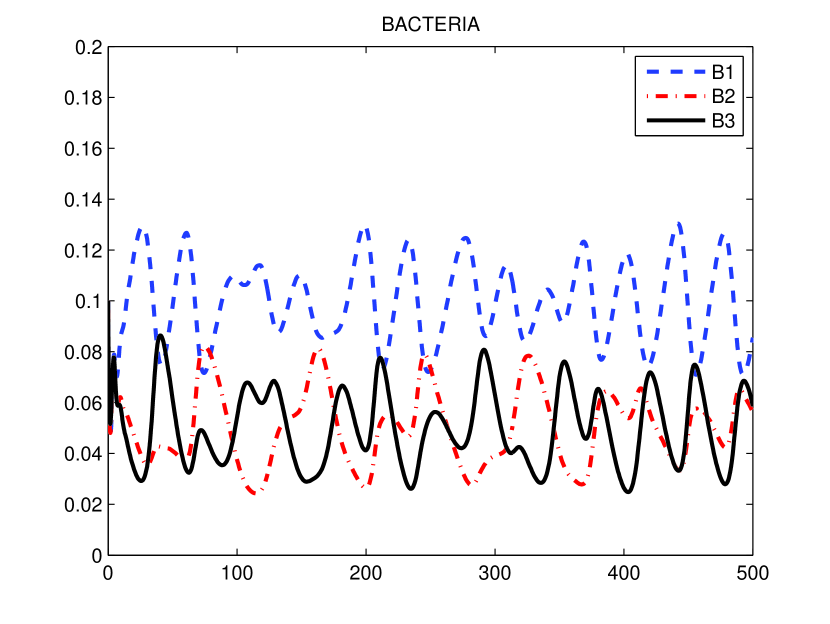
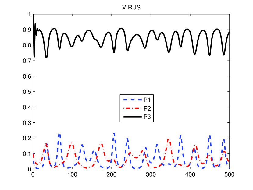
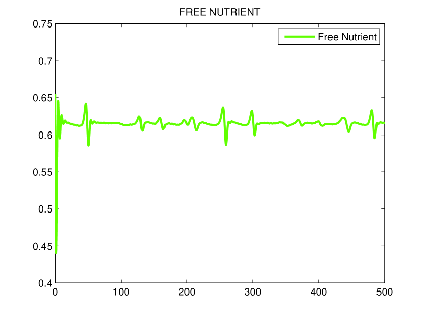
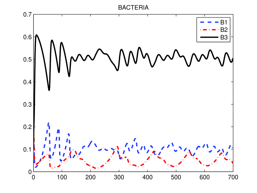
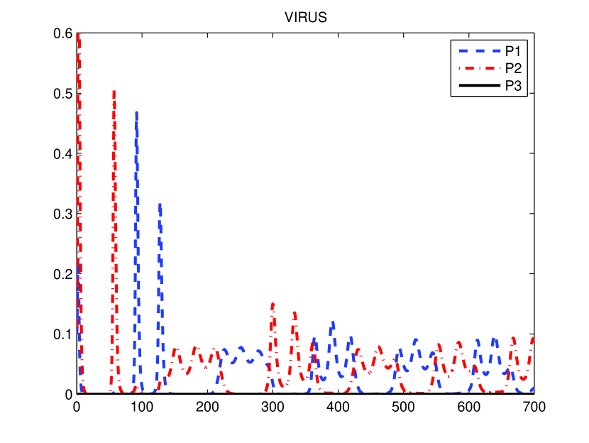
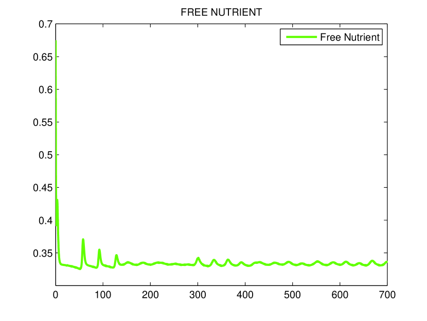
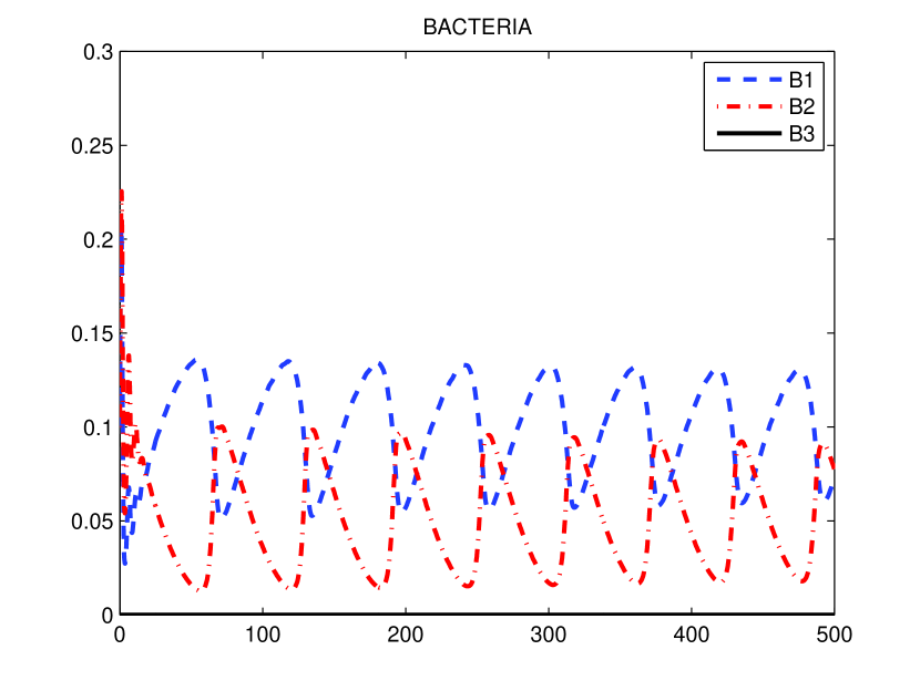
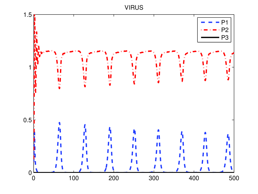
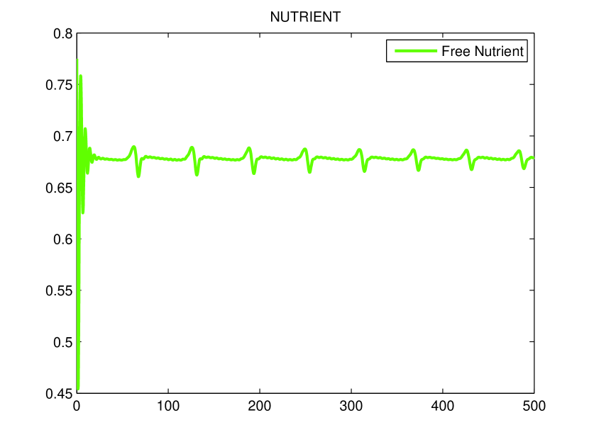
Figure 1. Top row: $B_{i}(0)=P_{i}(0)=0.1,1\leq i\leq 3$; second row: same except $P_{3}\equiv 0$; bottom row, as above except $B_{3}=P_{3}\equiv 0$.

4. Permanence

In this section we state and prove our main results, Theorem 4.7 and Corollary 4.8. We begin by establishing a competitive exclusion principle in the context of our model.

Two virus strains cannot share the same set of host bacterial strains; the weaker virus strain, the one with largest index, is doomed to extinction. This is due to our assumption that each virus strain does not distinguish among the host that it infects in terms of adsorption rate or burst size. Similarly, two bacteria strains cannot share the same set of infecting virus strains; the bacterial strain which is the least competitive for nutrient, the one with largest index, is doomed to extinction. The next result formalizes these conclusions.

Lemma 4.1 (Competitive Exclusion Principle).

Let $1\leq i<j\leq n$.

If $P_{i}(0)>0,P_{j}(0)>0$ and $B_{k}(0)=0,\ i<k\leq j$, then $P_{j}(t)\to 0$ as $t\to\infty$.

If $B_{i}(0)>0,B_{j}(0)>0$ and $P_{k}(0)=0,\ i\leq k<j$, then $B_{j}(t)\to 0$ as $t\to\infty$.

Proof.

The first assertion follows from Lemma 3.1 [11], applied to the equations for $P_{i}$ and $P_{j}$, where $\kappa_{1}=1/s_{i},\ \kappa_{2}=1/s_{j},\ h_{1}(t)=h_{2}(t)\equiv-1$, and $g(t)=\sum_{k\leq i}B_{k}(t)=\sum_{k\leq j}B_{k}(t)$. Note that

$$s_{j}\int_{0}^{t}h_{2}(s)ds-s_{i}\int_{0}^{t}h_{1}(s)ds=(s_{i}-s_{j})t\to-\infty.$$

Hence the result follows from the quoted result since $P_{i}(t)$ is bounded.

The second assertion also follows from Lemma 3.1, applied to the equations for $B_{i}$ and $B_{j}$, where $\kappa_{1}=\kappa_{2}=1$, $g(t)=\sum_{k\geq i}P_{k}(t)=\sum_{k\geq j}P_{k}(t)$, and $h_{1}=r_{i}-1-r_{i}U,\ h_{2}=r_{j}-1-r_{j}U$ where $U=\sum_{k}(B_{k}+s_{k}P_{k})$. Note that

$$\int_{0}^{t}h_{2}(s)-h_{1}(s)ds=(r_{j}-r_{i})\int_{0}^{t}(1-U(s))ds\to-\infty,$$

where the concluded limit is due to Lemma 4.3 and (2.5). ∎

Remark 4.2.

Lemma 4.1 strongly constrains the evolution of bacteria and virus communities, at least under our assumption that virus do not distinguish among their host in terms of adsorption rate and burst size. For example if a community consisting of a single virus strain and a single bacterial strain is invaded by a new virus strain then either the resident virus strain or the invader must be driven to extinction. However, our community can be successfully invaded by a new bacterial strain which is resistent to the virus but an inferior competitor for nutrient than the resident.

Hereafter, we assume without further mention that (3.1) holds.

If $h:(a,\infty)\to\mathbb{R}$, we write $h_{\infty}=\liminf_{t\to\infty}h(t)$ and $h^{\infty}$ with limit superior in place of limit inferior.

Lemma 4.3.

Every solution of (2.6) starting in $\Omega$ satisfies

(4.1) $$\limsup_{t\to\infty}U(t)\leq\frac{W^{\infty}}{1+W^{\infty}}\leq\frac{r_{1}}{1+r_{1}}$$

where $U=\sum_{i}(B_{i}+s_{i}P_{i})$ and $W=\sum_{i}r_{i}B_{i}$ are defined by (2.7).

Proof.

Apply the fluctuation lemma, e.g. Prop. A.14 [12], to (2.7) and use (2.5) and the invariance of $\Omega$ to conclude that $\sum_{j}B_{j}\leq 1$. ∎

Proposition 4.4.

If $P_{i}(0)>0$, then $(\sum_{j\leq i}B_{j})_{\infty}\leq s_{i}$.

If $B_{1}(0),P_{n}(0)>0$, then

(4.2) $$\left(\sum_{j}(r_{1}s_{j}+1)P_{j}\right)^{\infty}\geq r_{1}-1-r_{1}s_{n}>0.$$

1. If $(\sum_{j\leq i}B_{j})^{\infty}<s_{i}$ then $P_{i}(t)\to 0$.
   

2. If $i<j$, $P_{i}(0)>0$, and if $(B_{i+1}+B_{i+2}+\cdots+B_{j})^{\infty}<s_{j}-s_{i}$, then $P_{j}(t)\to 0$.
   

3. If $i<j$, $B_{i}(0)>0$, and if $(P_{i}+P_{i+1}+\cdots+P_{j-1})^{\infty}<\frac{r_{i}-r_{j}}{1+r_{1}}$, then $B_{j}(t)\to 0$.
   

Proof.

The equation for $P_{i}$ implies that

$$\frac{d}{dt}\log P_{i}^{s_{i}}(t)=\sum_{j\leq i}B_{j}-s_{i}.$$

If $(\sum_{j\leq i}B_{j})_{\infty}\leq s_{i}$ is false, then $P_{i}(t)\to\infty$, a contradiction to boundedness of solutions. Assertion (a) is transparent.

(3.4) implies that $r_{n}(1-s_{n})-1=r_{n}-1-r_{n}s_{n}>0$ and, with (2.3),(2.5) together, imply that $r_{1}-1-r_{1}s_{n}>0$. We have

$$\frac{B_{1}^{\prime}}{B_{1}}=r_{1}-1-r_{1}\sum_{j}B_{j}-\sum_{j}(r_{1}s_{j}+1)P_{j}$$

and

$$\frac{s_{n}P_{n}^{\prime}}{P_{n}}=\sum_{j}B_{j}-s_{n}.$$

Multiplying the second expression by $r_{1}$ and adding to the first gives

$$\frac{d}{dt}\log B_{1}P_{n}^{r_{1}s_{n}} = \frac{B_{1}^{\prime}}{B_{1}}+\frac{r_{1}s_{n}P_{n}^{\prime}}{P_{n}}$$

$$= r_{1}-1-r_{1}s_{n}-\sum_{j}(r_{1}s_{j}+1)P_{j}$$

(4.2) follows since the alternative is that $B_{1}P_{n}$ is unbounded, a contradiction.

Proof of (b): if $i<j$, $P_{i}(0)>0,P_{j}(0)>0$, and if $(B_{i+1}+\cdots+B_{j})^{\infty}<s_{j}-s_{i}$, then

$$\frac{d}{dt}\log\frac{P_{i}^{s_{i}}(t)}{P_{j}^{s_{j}}(t)} = \frac{s_{i}P_{i}^{\prime}}{P_{i}}-\frac{s_{j}P_{j}^{\prime}}{P_{j}}$$

$$= -(B_{i+1}+\cdots+B_{j})+s_{j}-s_{i}$$

$$\geq \epsilon,\ t\geq T$$

for some $\epsilon,T>0$. Therefore, $\frac{P_{i}^{s_{i}}(t)}{P_{j}^{s_{j}}(t)}\to\infty$, which implies that $P_{j}(t)\to 0$ since $P_{i}(t)$ is bounded.

proof of (c): assume that $B_{i}(0)>0,B_{j}(0)>0$, and $(P_{i}+P_{i+1}+\cdots+P_{j-1})^{\infty}<\frac{r_{i}-r_{j}}{1+r_{1}}$. Then, recalling that $U=\sum_{k}(B_{k}+s_{k}P_{k})$, we have

$$\frac{d}{dt}\log\frac{B_{i}(t)}{B_{j}(t)} = \frac{B_{i}^{\prime}}{B_{i}}-\frac{B_{j}^{\prime}}{B_{j}}$$

$$= (r_{i}-r_{j})(1-U)-(P_{i}+P_{i+1}+\cdots+P_{j-1})$$

$$\geq (r_{i}-r_{j})\left(\frac{1-\epsilon}{1+r_{1}}\right)-(P_{i}+P_{i+1}+\cdots+P_{j-1}),\ t\geq T$$

where, by (4.1), we can choose $\epsilon>0$ so small that $(P_{i}+P_{i+1}+\cdots+P_{j-1})^{\infty}<(r_{i}-r_{j})(\frac{1-\epsilon}{1+r_{1}})$. It follows that $B_{i}/B_{j}\to\infty$ which implies that $B_{j}(t)\to 0$.

∎

Note that case (b) and (c) of Proposition 4.4 extend Lemma 4.1.

Proposition 4.5.

If $B_{1}(0)>0$, then $B_{1}^{\infty}\geq s_{1}$.

If $B_{1}(0)>0$ and $P_{1}(0)>0$, then

$$B_{1}^{\infty}\geq s_{1},\ P_{1}^{\infty}\geq\min\{\frac{r_{1}-r_{2}}{1+r_{1}},\frac{r_{1}-1-r_{1}s_{1}}{r_{1}s_{1}+1}\}.$$

Proof.

Assume the conclusion is false. Then $P_{1}\to 0$ by Proposition 4.4 (a). If $P_{i}(0)=0$ for all $i$, then $B_{1}(t)\to 1-1/r_{1}\geq s_{1}$ by the classical chemostat theory, e.g. Theorem 3.2 in [14], so we suppose that $P_{i}(0)>0$ for some $i$. Let $k$ denote the smallest such integer $i$ for which $P_{i}(0)>0$.

If $k=1$, then, as noted above, $P_{1}\to 0$ and so $B_{2}\to 0$ by Proposition 4.4 (c). Then $P_{2}\to 0$ by Proposition 4.4 (a) or (b).

If $k=2$, then $P_{1}\equiv 0$ so $B_{2}\to 0$ by Lemma 4.1 since $B_{1}$ and $B_{2}$ share the same virus. Since $(B_{1}+B_{2})^{\infty}=B_{1}^{\infty}<s_{1}<s_{2}$, it follows that $P_{2}\to 0$ by Proposition 4.4 (a). Now we can use Proposition 4.4 (c) to show $B_{3}\to 0$ and then Proposition 4.4 (a) or (b) to show $P_{3}\to 0$.

If $k>2$, then $P_{1}\equiv P_{2}\equiv\cdots\equiv P_{k-1}\equiv 0$ and $P_{k}(0)>0$. As $B_{1},\cdots,B_{k-1}$ share the same virus, then $B_{i}\equiv 0$ or $B_{i}\to 0$ for $1<i\leq k-1$ by Lemma 4.1. $B_{k}\to 0$ by Proposition 4.4 (c). Then, $P_{k}\to 0$ by Proposition 4.4 (a) since $(\sum_{j\leq k}B_{j})^{\infty}=B_{1}^{\infty}<s_{1}<s_{k}$. So $B_{k+1}\to 0$ by Proposition 4.4 (c). Proposition 4.4 (a) or (b) implies that $P_{k+1}\to 0$.

We see that for all values of $k$, $B_{2},\cdots,B_{k+1}\to 0$ and $P_{1},\cdots,P_{k+1}\to 0$. Successive additional applications of Proposition 4.4 (a) or (b) and (c) then imply that $B_{2},\cdots,B_{n}\to 0$ and $P_{1},\cdots,P_{n}\to 0$. But, then

$$B_{1}^{\prime}/(r_{1}B_{1})\geq 1-\frac{1}{r_{1}}-\epsilon-B_{1}>s_{1}+\epsilon-B_{1},\ t\geq T$$

for some $\epsilon>0$ and $T>0$ (recall that $s_{1}<1-1/r_{1}$). This implies that $B_{1}^{\infty}>s_{1}$, a contradiction. This completes the proof of the first assertion.

Now, suppose that $B_{1}(0)>0,P_{1}(0)>0$ and $P_{1}^{\infty}<\frac{r_{1}-r_{2}}{1+r_{1}}$. Proposition 4.4 (c) implies that $B_{2}\to 0$. By Proposition 4.4 (b), $P_{2}\to 0$. Applying Proposition 4.4 (c) with $i=1$ and $j=3$, as $(P_{1}+P_{2})^{\infty}=P_{1}^{\infty}<\frac{r_{1}-r_{2}}{1+r_{1}}<\frac{r_{1}-r_{3}}{1+r_{1}}$, we conclude that $B_{3}\to 0$. Then, Proposition 4.4 (b) implies that $P_{3}\to 0$. Clearly, we can continue sequential application of Proposition 4.4 (b) and (c) to conclude that $B_{i},P_{i}\to 0$ for $i>1$. Now, we may argue as in the proof of (4.2)

$$\frac{d}{dt}\log B_{1}P_{1}^{r_{1}s_{1}} = \frac{B_{1}^{\prime}}{B_{1}}+\frac{r_{1}s_{1}P_{1}^{\prime}}{P_{1}}$$

$$= r_{1}-1-r_{1}s_{1}-(r_{1}s_{1}+1)P_{1}-\hbox{terms that go to zero}$$

to conclude that $P_{1}^{\infty}\geq\frac{r_{1}-1-r_{1}s_{1}}{1+s_{1}r_{1}}$.

∎

The following is a slight modification of Theorem 5.2.3 in [6].

Lemma 4.6.

Let $x(t)$ be a bounded positive solution of the Lotka-Volterra system

$$x_{i}^{\prime}=x_{i}(r_{i}+\sum_{j=1}^{n}a_{ij}x_{j}),\ 1\leq i\leq n$$

and suppose there exists $k<n$ and $m,M,\delta>0$ such that $m\leq x_{i}(t)\leq M,\ 1\leq i\leq k,\ t>0$, $x_{k+1}(t)\leq\delta,\ t>0$, and $x_{j}(t)\to 0$ for $j>k+1$. Suppose also that the $k\times k$ subsystem obtained by setting $x_{j}=0,j>k$ has a unique positive equilibrium $p=(p_{1},p_{2},\cdots,p_{k})$. Then

$$\liminf_{T\to\infty}\frac{1}{T}\int_{0}^{T}x_{i}(t)dt=p_{i}+O(\delta),\ 1\leq i\leq k.$$

The same expression holds for the limit superior.

Proof.

As in [6] Thm 5.2.3, we have that $z_{j}(T)=\frac{1}{T}\int_{0}^{T}x_{j}(t)dt$ satisfies

$$\frac{\log x_{i}(T)-\log x_{i}(0)}{T}=\sum_{i=1}^{k}a_{ij}(z_{j}(T)-p_{j})+a_{i(k+1)}z_{k+1}(T)+\sum_{j>k+1}a_{ij}z_{j}(T).$$

for $i=1,2,\cdots,k$. As $T\to\infty$, the left hand side converges to zero and so does the final sum on the right since $x_{j}\to 0$ for $j>k+1$. The $k\times k$ matrix $\tilde{A}=(a_{ij})_{1\leq i,j\leq k}$ is invertible by hypothesis so we may write the above in vector form as

$$z(T)=p+(\tilde{A})^{-1}(O(1/T)-z_{k+1}(T)A_{k+1})$$

where $O(1/T)\to 0$ and $A_{k+1}$ is the first $k$ entries of the $k+1$ column of $A=(a_{ij})_{1\leq i,j\leq n}$. As $0\leq z_{k+1}\leq\delta$, it follows that $\|z(T)-p\|\leq c\delta$ for some $c$ and all large $T$. The result follows. ∎

Our main result follows.

Theorem 4.7.

Let $1\leq k\leq n$.

1. There exists $\epsilon_{k}>0$ such that if $B_{i}(0)>0,\ 1\leq i\leq k$ and $P_{j}(0)>0,\ 1\leq j\leq k-1$, then

   $$B_{i,\infty}\geq\epsilon_{k},\ 1\leq i\leq k\ \hbox{and}\ P_{j,\infty}\geq\epsilon_{k},\ 1\leq j\leq k-1.$$

2. There exists $\epsilon_{k}>0$ such that if $B_{i}(0)>0,P_{i}(0)>0,\ 1\leq i\leq k$, then

   $$B_{i,\infty}\geq\epsilon_{k},\ P_{i,\infty}\geq\epsilon_{k},\ 1\leq i\leq k.$$

Proof.

We use the notation $[B_{i}]_{t}\equiv\frac{1}{t}\int_{0}^{t}B_{i}(s)ds$. Our proof is by mathematical induction using the ordering of the $2n$ cases as follows

$$(a,1)<(b,1)<(a,2)<(b,2)<\cdots<(a,n)<(b,n)$$

where $(a,k)$ denotes case (a) with index $k$.

The cases $(a,1)$ and $(b,1)$ follow immediately from Proposition 4.5 and by the general result that weak uniform persistence implies strong uniform persistence under suitable compactness assumptions. See Prop. 1.2 in [15] or Corollary 4.8 in [12] with persistence function $\rho=\min\{B_{1},P_{1}\}$ in case $(b,1)$. Note that our state space is compact.

For the induction step, assuming that $(a,k)$ holds, we prove that $(b,k)$ holds and assuming that $(b,k)$ holds, we prove that $(a,k+1)$ holds.

We begin by assuming that $(a,k)$ holds and prove that $(b,k)$ holds. We consider solutions satisfying $B_{i}(0)>0,P_{i}(0)>0$ for $1\leq i\leq k$. Note that other components $B_{j}(0)$ or $P_{j}(0)$ for $j>k$ may be positive or zero, we make not assumptions. As $(a,k)$ holds, there exists $\epsilon_{k}>0$ such that $B_{i,\infty}\geq\epsilon_{k},\ 1\leq i\leq k$ and $P_{i,\infty}\geq\epsilon_{k},\ 1\leq i\leq k-1$. We need only show the existence of $\delta>0$ such that $P_{k,\infty}\geq\delta$ for every solution with initial values as described above. In fact, by the above-mentioned result that weak uniform persistence implies strong uniform persistence, it suffices to show that $P_{k}^{\infty}\geq\delta$.

If $P_{k}^{\infty}<\frac{r_{k}-r_{k+1}}{1+r_{1}}$, then $B_{k+1}\to 0$ by Proposition 4.4 (c). Then, by Proposition 4.4 (b), $P_{k+1}\to 0$. Clearly, we may sequentially apply Proposition 4.4 (b) and (c) to show that $B_{j}\to 0,P_{j}\to 0$ for $j\geq k+1$.

If there is no $\delta>0$ such that $P_{k}^{\infty}\geq\delta$ for every solution with initial data as described above, then for every $\delta>0$, we may find a solution with such initial data such that $P_{k}^{\infty}<\delta$. By a translation of time, we may assume that $P_{k}(t)\leq\delta,\ t\geq 0$ for $0<\delta<\frac{r_{k}-r_{k+1}}{1+r_{1}}$ to be determined later. Then $B_{j},P_{j}\to 0,j\geq k+1$. Now, as $(a,k)$ holds, we may apply Lemma 4.6. The subsystem with $B_{i}=0,\ k+1\leq i\leq n$ and $P_{i}=0,\ k\leq i\leq n$ has a unique positive equilibrium by Proposition 3.1. See Remark 3.3. The equation

$$\frac{s_{k}P_{k}^{\prime}}{P_{k}}=\sum_{j\leq k}B_{j}-s_{k}$$

implies that

$$\frac{1}{t}\log\frac{P_{k}^{s_{k}}(t)}{P_{k}^{s_{k}}(0)}=\sum_{j\leq k}[B_{j}]_{t}-s_{k}.$$

By (3.1) and Lemma 2.6, we have for large $t$

$$\sum_{j\leq k}[B_{j}]_{t}=\sum_{j\leq k}B_{j}^{\dagger}+O(\delta)=s_{k}+q+O(\delta)$$

where $q=(1-\frac{1+Q_{k}}{r_{k}})>0$. On choosing $\delta$ small enough and an appropriate solution, then $\sum_{j\leq k}[B_{j}]_{t}-s_{k}>q/2$ for large $t$, implying that $P_{k}\to+\infty$, a contradiction. We have proved that $(a,k)$ implies $(b,k)$.

Now, we assume that $(b,k)$ holds and prove that $(a,k+1)$ holds. We consider solutions satisfying $B_{i}(0)>0,P_{i}(0)>0$ for $1\leq i\leq k$ and $B_{k+1}(0)>0$. As $(b,k)$ holds by assumption, and following the same arguments as in the previous case, we only need to show that there exists $\delta>0$ such that $B_{k+1}^{\infty}\geq\delta$ for all solutions with initial data as just described.

If $B_{k+1}^{\infty}<s_{k+1}-s_{k}$, then $P_{k+1}\to 0$ by Proposition 4.4 (b) and then $B_{k+2}\to 0$ by Proposition 4.4 (c). This reasoning may be iterated to yield $B_{i}\to 0,\ k+2\leq i\leq n$ and $P_{i}\to 0,\ k+1\leq i\leq n$.

If there is no $\delta>0$ such that $B_{k+1}^{\infty}\geq\delta$ for every solution with initial data as described above, then for every $\delta>0$, we may find a solution with such initial data such that $B_{k+1}^{\infty}<\delta$. By a translation of time, we may assume that $B_{k+1}(t)\leq\delta,\ t\geq 0$ for $0<\delta<s_{k+1}-s_{k}$ to be determined later. Then $B_{j},P_{j}\to 0,j\geq k+2$ and $P_{k+1}\to 0$. Now, using that $(b,k)$ holds, we apply Lemma 4.6. The subsystem with $B_{i}=0,P_{i}=0\ k+1\leq i\leq n$ has a unique positive equilibrium by Proposition 3.1. See Remark 3.3. The equation for $B_{k+1}$ is

$$\frac{B_{k+1}^{\prime}}{B_{k+1}}=r_{k+1}-1-r_{k+1}\sum_{j=1}^{k}(B_{j}+s_{j}P_{j})-r_{k+1}\sum_{j=k+1}^{n}(B_{j}+s_{j}P_{j})-\sum_{j=k+1}^{n}P_{j}$$

Integrating, we have

$$\frac{1}{t}\log\frac{B_{k+1}(t)}{B_{k+1}(0)}=r_{k+1}-1-r_{k+1}\sum_{j=1}^{k}([B_{j}]_{t}+s_{j}[P_{j}]_{t})-r_{k+1}[B_{k+1}]_{t}+O(1/t)$$

By (3.2) and Lemma 4.6, we have that for all large $t$

$$\sum_{j=1}^{k}([B_{j}]_{t}+s_{j}[P_{j}]_{t})=\sum_{j=1}^{k}(B_{j}^{*}+s_{j}P_{j}^{*})+O(\delta)=\frac{Q_{k}}{1+Q_{k}}+O(\delta).$$

Since $B_{k+1}(t)\leq\delta$, $[B_{k+1}]_{t}=O(\delta)$. Hence, for large $t$

$$\frac{1}{t}\log\frac{B_{k+1}(t)}{B_{k+1}(0)}=\frac{r_{k+1}}{1+Q_{k}}-1+O(\delta)+O(1/t).$$

Now, $\frac{r_{k+1}}{1+Q_{k}}>\frac{r_{k+1}}{1+Q_{k+1}}>1$ so by choosing $\delta$ sufficiently small and an appropriate solution, we can ensure that the right hand side is bounded below by a positive constant for all large $t$, implying that $B_{k+1}(t)$ is unbounded. This contradiction completes our proof that $(b,k)$ implies $(a,k+1)$. Thus, our proof is complete by mathematical induction. ∎

Corollary 4.8.

For every solution of (2.6) starting with all components positive, we have that

(4.3) $$\frac{1}{t}\int_{0}^{t}B_{i}(s)ds\to B_{i}^{*},\ \frac{1}{t}\int_{0}^{t}P_{i}(s)ds\to P_{i}^{*}$$

where $B_{i}^{*},P_{i}^{*}$ are as in (3.2).

For every solution of (2.6) starting with all components positive except $P_{n}(0)=0$, we have that

(4.4) $$\frac{1}{t}\int_{0}^{t}B_{i}(s)ds\to B_{i}^{\dagger},\ \frac{1}{t}\int_{0}^{t}P_{i}(s)ds\to P_{i}^{\dagger}$$

where $B_{i}^{\dagger},P_{i}^{\dagger}$ are as in (3.1).

Proof.

This follows from the previous theorem together with Theorem 5.2.3 in [6]. ∎

References

- [1] B. Bohannan and R. Lenski, Linking genetic change to community evolution: insights from studies of bacteria and bacteriophages, Ecology Letters (2000) 3, 362-377.
- [2] L. Chao, B. Levin, F. Stewart, A Complex Community in a Simple Habitat: An Experimental Study with Bacteria and Phage, Ecology (1977) 58, 369-378.
- [3] B. Garay and J. Hofbauer, Robust Permanence for ecological differential equations, minimax, and discretizations, SIAM J. Math. Anal. (2003) 34, 1007-1039.
- [4] Z. Han and H. Smith, Bacteriophage-Resistant and Bacteriophage-Sensitive Bacteria in a Chemostat, Math. Biosciences and Eng. 9, No. 4, 2012, 737-765.
- [5] M. Hirsch, H. Smith, X.-Q. Zhao, Chain transitivity, attractivity and strong repellors for semidynamical systems, J.Dynamics and Diff. Eqns. 13, 2001, 107-131.
- [6] J. Hofbauer and K. Sigmund, Evolutionary games and Population Dynamics, Cambridge Univ. Press, 1998.
- [7] L. F. Jover, M.H. Cortez, J.S. Weitz, Mechanisms of multi-strain coexistence in host phage systems with nested infection networks. Journal of Theoretical Biology 332 (2013) 65-77
- [8] R. Law and R. Morton, Permanence and the assembly of ecological communities, Ecology 77(3), 1996, 762-775.
- [9] R. May and W. Leonard, Nonlinear aspects of competition between three species, SIAM J. Applied Math. 29 (1975), 243-253.
- [10] S. Schreiber, Criteria for robust permanence, J. Diff. Eqns. 162, (2000), 400-426.
- [11] H. Smith and H. Thieme, Chemostats and epidemics:competition for nutrients or host, with H. Thieme, Mathematical Bioscience and Engineering (10) December 2013, 1635-1650.
- [12] H. Smith and H. Thieme, Dynamical Systems and Population Persistence, GSM 118, Amer. Math. Soc. , Providence R.I., 2011.
- [13] H. Smith and H. Thieme, Persistence of Bacteria and Phages in a Chemostat, Journal of Mathematical Biology: Volume 64, Issue 6 (2012), Page 951-979
- [14] H. Smith and P. Waltman, The Theory of the Chemostat, Cambridge Univ. Press, 1995.
- [15] H. Thieme, Persistence under relaxed point-dissipativity (with applications to an endemic model), SIAM J. Math. Anal., 24 (1993), 407-435.
- [16] D. Tilman, Resource Competition and Community Structure, Princeton Univ. Press, Princeton N.J. (1982).
- [17] J. Weitz, H. Hartman, S. Levin, Coevolutionary arms races between bacteria and bacteriophage, PNAS 102 (2005) 9535-9540.