semileptonic decay form factors with disconnected quark loop contributions
Abstract
We calculate for the first time the form factors of the semileptonic decays of the meson to and using lattice techniques. As a by-product of the calculation we obtain the masses and leading distribution amplitudes of the and mesons. We use non-perturbatively improved clover fermions on configurations with a lattice spacing fm. We are able to obtain clear signals for relevant matrix elements, using several noise reduction techniques, both for the connected and disconnected contributions. This includes a new method for reducing the variance of pseudoscalar disconnected two-point functions. At zero momentum transfer, we obtain for the scalar form factors, and at , as well as and at , where the errors are statistical only.
pacs:
12.38.Gc, 13.20.Fc, 14.40.Lb, 14.40.BeI Introduction
In general, semileptonic decays of charmed mesons are well studied both experimentally and theoretically, in particular, using lattice techniques. However, this is not the case for the meson for which the main semileptonic modes are to the , and mesons. Lattice studies of these decays are technically challenging due to the presence of disconnected quark-line contributions. So far only the form factor for the decay has been computed, omitting the disconnected contributions Donald et al. (2014). QCD sum rules provide an alternative approach based on the operator product expansion (OPE) and analyticity using the assumption of quark-hadron duality. There is one result using the standard local OPE in terms of condensates Colangelo and De Fazio (2001) and two using light cone OPE in terms of distribution amplitudes Azizi et al. (2011); Offen et al. (2013). These studies utilize the and distribution amplitudes, which, in principle, can be calculated on the lattice. A first principles calculation of the form factors for therefore can serve as a cross-check on the assumptions of the sum rule approach and is of phenomenological interest in itself, providing information on the internal structure of the mesons in the final state (see, for example, Ref. Di Donato et al. (2012)). In terms of experimental results, there are no measurements of the form factors for these modes so far and only the branching fractions for have been determined by the CLEO collaboration Yelton et al. (2009).
In this article, we report on our exploratory study of the to semileptonic decay form factors using lattice techniques. Some preliminary results have been presented in Refs. Kanamori (2012); Collins et al. (2013, 2014). The relevant matrix elements for these decay modes are parameterized as follows
| (1) |
where is a vector current at position111In practice one averages over all positions , injecting the spatial momentum required by momentum conservation, to increase statistics. , is the four-momentum transfer and and are the masses of the and the mesons, respectively. This matrix element is characterized by two form factors, and . In this work we focus on the scalar form factor , which we can also obtain from a scalar current Na et al. (2010):
| (2) |
We use this relation because the combination (and therefore ) is a renormalization group invariant, provided the vector mass difference is used. Eq. (2) is also free of additive renormalization.
The three-point function needed to compute the form factor contains quark-line disconnected loops (see Fig. 1). Often corrections from disconnected loops are numerically small. However, their impact on the three-point function is enhanced by a factor of about three, due to the summation over three light quark flavours. Moreover, in the pseudoscalar case the disconnected quark loops couple to the axial anomaly. In spite of the computational expense and the inferior quality of the signal, relative to that of the quark-line connected contribution, the calculation of the disconnected contribution turns out to be feasible and its impact is significant Bali et al. (2011a); Kanamori (2012). Therefore, these decay modes also provide a perfect playground for testing a variety of techniques for calculating the disconnected quark-line loops.
We use QCDSF configurations Bietenholz et al. (2010, 2011) that were generated using a novel approach for varying the sea quark masses, which is ideal for studying flavour physics in the SU(3) flavour basis. The flavour singlet mass average of the three light quarks, , is kept fixed so that the combination computed from the kaon mass, , and pion mass, , approximately coincides with the physical value. Starting from the flavour SU(3) symmetric point (), is reduced as is increased.
The outline of this paper is as follows: in the next Section we describe the technical details of the lattice calculation. Before we can address decays of the meson into final states including the or mesons, we have to construct the corresponding interpolators. Therefore, in Section III, we determine the mixing of the physical states relative to the octet-singlet basis. We present a new method to reduce statistical noise and obtain the and masses and the leading distribution amplitudes. The details of the new method, described in Subsection III.2, are quite technical and can be skipped by those readers who are primarily interested in the final results. In Section IV we describe our methods for extracting the matrix elements relevant for the computation of the form factors. Subsequently, these are obtained in the same Section, before we conclude.
II Details of the lattice calculation
The QCDSF configurations were generated with the tree level Symanzik improved gluon action and the Stout Link Non-perturbatively improved Clover fermion action (SLiNC) Cundy et al. (2009). We use the same action for the valence-only charm quark. The SLiNC action is on-shell improved. In general, there will be correction term, , to Eq. (2). However, this term can be eliminated using the equations of motion and one can show that the non-singlet improvement coefficients Sint and Weisz (1998); Bhattacharya et al. (2006) cancel from Eq. (2) so that is automatically -improved.
The parameters are summarized in Table 1. So far we have only used one lattice spacing (determined using the quantity proposed in Ref. Borsanyi et al. (2012)), and one volume , which corresponds to a physical spatial extent . Our value of the lattice spacing is about 10% smaller than the value of Refs. Bietenholz et al. (2010, 2011) () which was obtained from the average octet baryon mass, but is consistent with a newer determination () in Ref. Horsley et al. (2013). We analyzed 939 configurations at the flavour symmetric point (), for which (Set S), and 239 configurations () with and (Set A). Due to the different value for the lattice spacing, these masses differ from the numbers given in Refs. Bietenholz et al. (2010, 2011). In particular, the average octet pion mass exceeds the experimental value by about , meaning that extrapolating to the physical pion mass, we would end up with unphysically heavy kaons. The charm quark mass was tuned so that the spin averaged 1S charmonium mass, , corresponds to the experimental value Bali et al. (2011b).
In order to reduce autocorrelations, the configurations were sampled every 5 Monte Carlo trajectories for Set S and every 10 trajectories for Set A. In addition, the location of the source was chosen randomly on each configuration. However, significant correlations were found in the data when calculating the masses of the , and mesons, and we chose a conservative bin size of 5 (25 molecular dynamics time units) for Set S and 2 (20 molecular dynamics time units) for Set A. The mass of the , the mixing angle discussed in Sec. III.3 and the form factor, , did not show any significant autocorrelations, so we did not use binning for these observables.
For all source and sink interpolators, we used a gauge invariant Gaussian smearing (Wuppertal smearing Güsken et al. (1989); Güsken (1990)) with APE smeared gauge fields Falcioni et al. (1985) in the spatial directions. The smearing parameters were chosen to minimize excited state contributions to the connected two-point functions.
| Set | confs. | |||||
|---|---|---|---|---|---|---|
| S | 5.5 | 0.12090 | 0.12090 | 4.3 | 939 | |
| A | 5.5 | 0.12104 | 0.12062 | 3.3 | 239 |
Disconnected fermion loops appear in both two- and three-point functions. These loops need to be evaluated at different times and momenta. They can be obtained from the inverse of the dimensionless lattice Dirac operator, , in the following way:
| (3) |
where the Dirac matrix for a pseudoscalar meson is and is the smearing function. The origin for the Fourier transformation is denoted as . Since satisfies -Hermiticity, the smearing function is Hermitian and commutes with , the disconnected loop is real in coordinate space and . Details of the estimation of the disconnected loops are given in Appendix A.
III and states
Prior to determining decays of the into the or mesons, we have to construct these physical states. We first discuss the general mixing formalism, relative to the octet-singlet basis, then determine the respective masses and compare our results to other studies. In Section III.2, which is technical and can be skipped on first reading, we discuss a particular problem we encountered, due to the insufficient sampling across topological sectors on one of our ensembles. The method we suggest to resolve this turns out to be of a more general applicability and significantly reduces statistical errors. Finally, in Section III.3 we determine mixing angles and leading distribution amplitudes of these states.
III.1 Extracting physical states
The correct creation operators for the and states are a priori unknown in the flavour non-symmetric case (Set A). We start from singlet and octet states and first calculate a correlation matrix of two-point functions222We always use for expectation values so that the correlation functions without like and denote configuration by configuration quantities.
| (4) |
where and are smeared interpolators for the octet and singlet states, respectively. Each element includes disconnected fermion loop contributions. The latter were averaged over all possible source positions in space and time, shifting the source and the sink accordingly. For the connected part, we used low mode averaging DeGrand and Schäfer (2004); Giusti et al. (2004). We describe the details of these calculations in Appendix B. We solve the following generalized eigenvalue problem
| (5) |
where () is the generalized eigenvalue and is the generalized eigenvector. The time slice can be varied to minimize the excited state contributions to and . We tried – and found no significant difference in the results, so we use which gives the largest range of . We parameterize the eigenvectors of the two-dimensional system in the following way
| (6) |
Note that in general . In the large limit, the ground state dominates, and we can obtain the interpolators for the physical ground states:
| (7) |
It is sufficient to extract and . This was done by fitting the corresponding components of to a constant, taking into account correlations including those between and and those between different time slices. Using Eq. (7), we can construct the two-point functions of the physical states for each :
| (8) |
The energy of the state at a momentum , , can then be obtained by fitting these two-point functions at sufficiently large times to the functional form
| (9) |
where is the temporal lattice extent, and is a (momentum-dependent) amplitude.
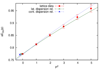
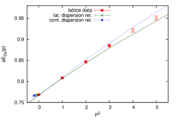
At zero momentum the situation is more involved and we deviate from the above procedure, see Section III.2. For the mass on Set A and Set S and the mass on Set A, the statistical error of could be further reduced by fitting zero- and non-zero-momentum data to the lattice dispersion relation
| (10) |
where the mass, , is a free parameter. This is illustrated in Fig. 2, where the energies we obtained directly at zero and at finite momenta, and the fitted dispersion relations and their results are shown. The masses are listed in Table 2, and the energies at zero and finite momenta in Tables 7 and 8 of Appendix D. The meson at the SU(3) flavour symmetric point (Set S) is identical to the pion (and the kaon) and the precision of its mass did not benefit from including non-zero momentum data. In this case we display the result in the table. No significant differences were found for the and masses if the continuum dispersion relation was used instead, as seen in the figure. For comparison, we also show the data in the figure. For this meson, the lattice dispersion relation is clearly preferred by the data: the from the correlated fit were poor (4.7 for Set S and 2.2 for Set A) and did not reproduce the data. In Fig. 2, uncorrelated fits are shown in these cases.
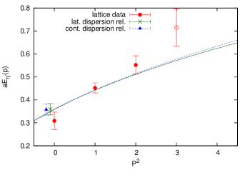
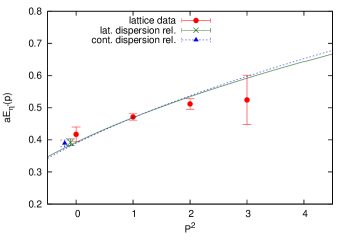
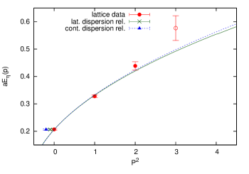
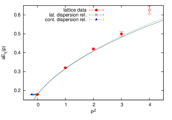
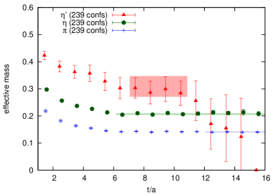
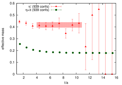
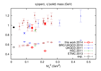
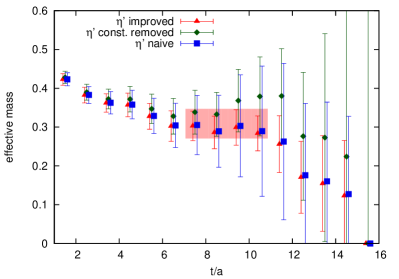
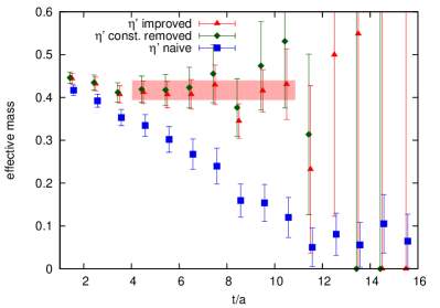
In Fig. 3, we plot the effective masses of the , the and the . The fitted and masses, with the exception of the at the SU(3) symmetric point, were obtained using the improved method detailed in the next subsection. The masses are and for Set S (), and for Set A (), where the errors are statistical only. These values are consistent with the finite momentum data shown in Fig. 2.
In Fig. 4 we compare our and masses to results obtained by other lattice collaborations Christ et al. (2010); Gregory et al. (2012); Dudek et al. (2011); Michael et al. (2013) and the respective experimental values Olive et al. (2014). In some of these studies the extrapolation to the physical point was performed, however, for consistency we do not show extrapolated values. Note that, since the flavour singlet quark mass average is kept fixed in our simulations, the mass of the approaches the physical point from below. Our results seem to approach the experimental values and the masses are consistent with other lattice determinations that were obtained keeping the strange quark mass approximately constant.
III.2 Finite volume effects on the and masses
Analysing Set S we found that the two-point function at large times does not decay to zero (cf. Eq. (9)) but instead saturates at a small non-zero value. This phenomenon can be explained as a finite volume effect, coupled to unrealistic fluctuations of the topological charge, due to an insufficient sampling of the topological sectors within our limited statistics. We will see that this can be cured by defining an improved observable which also reduces the variance of disconnected pseudoscalar two-point functions in the case of a correctly sampled topological charge.
The disconnected contributions can be obtained by correlating pairs of momentum-projected “1-point loops”. The sum over such a one-point loop is proportional to the fermionic definition of the topological charge :
| (11) |
where the (dimensionless) proportionality constant will depend on the quark mass, the smearing function and the normalization of the interpolator and we assume the fermionic and gluonic definitions of the topological charge to agree . The above relation suggests an approximate proportionality between the topological charge density and the fermionic one-point loop: .
If the topological charge is fixed to , point-point correlators of the topological charge density will remain finite for large separations Aoki et al. (2007):
| (12) |
where is the physical four-volume, is the topological susceptibility, and the dimensionful kurtosis parameterizes the leading deviations from Gaussian fluctuations of . Projecting the above expression onto a fixed spatial momentum, the constant term only affects the case.
Using , we obtain the following estimate of the two-point function, which is the singlet two-point function (see Eq. (61)) in the SU(3) flavour symmetric case:
| (13) |
Here is the quark-line connected part of the two-point function and is the temporal extent of the lattice. By using Eq. (12) and the observation that is negligible for our ensembles, we obtain
| (14) |
for large , resulting in the prediction for the finite volume effect at :
| (15) |
For the non-SU(3) flavour symmetric case, in principle, both the singlet and octet parts of the two-point function should contribute to the constant. However, using only the singlet part gives a good approximation because in Eq. (7) is small. The singlet-to-singlet contribution to the two-point function is
| (16) |
and we obtain
| (17) |
where we used a flavour-averaged proportionality constant333 For each flavour , we have , where the proportionality constant depends on the flavour through the quark mass. in Eq. (18) can be written as .
| (18) |
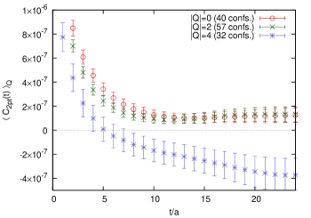
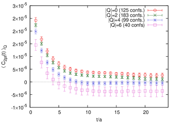
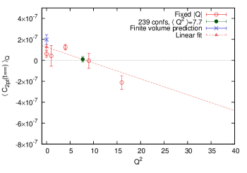
To check Eq. (14), we measured using an improved field strength tensor Bilson-Thompson et al. (2003) on smeared gauge fields with 90 iterations of Stout Morningstar and Peardon (2004) smearing. The measured values clustered around integer values as expected. For each integer , using configurations with only (we denote them as configurations), we calculated the two-point function of the at zero momentum. The values of the two-point functions in the large time limit exhibit a clear dependence on , see Fig. 5. Moreover, the constants obtained by fitting within such subsets are consistent with the linear dependence on suggested by Eq. (14), see Fig. 6. See Ref. Bali et al. (2001) for an earlier observation of the dependence of the effective mass, Ref. Brower et al. (2003) for the general argument and Ref. Kaneko et al. (2009) for a fixed topology approach.
In Fig. 6, we also plot the predictions. These were obtained from Eq. (15) (Set S) and Eq. (17) (Set A). The topological susceptibilities were computed using the gluonic definition of the topological charge and the parameters were obtained by fitting the one-point loops as a function of the gluonic topological charge as in Eq. (18). For Set A we find consistency between the linear extrapolation and this prediction. On Set S, however, the prediction is significantly smaller than the extrapolated value, and also smaller than the measured values. At the same time the two-point function, averaged over all configurations, approaches a non-zero (positive) value. The linear fit of the constant part versus crosses zero at a value . Replacing the measured value within Eq. (15) by , the prediction would be compatible with the fixed topology measurements. These observations are coherent with our above arguments and strongly suggest on Set S to be underestimated, due to an insufficient sampling.
While the distribution of on Set S is too narrow, we find within errors on both ensembles. Therefore, replacing within the above two-point functions will not affect any expectation value or correct for the sampling of topological sectors in Set S. Nevertheless, we checked whether this procedure reduced the statistical noise but we did not find any improvement.
One way of addressing the problem of a non-vanishing expectation value of the two-point function at large Euclidean times is simply to fit the correlation function to a constant plus an exponential decay (which we denote as “naive fit with a constant”). We adopted, however, a different strategy that we found to reduce the gauge noise: this is motivated by the results in Fig. 6, which suggest that the two-point functions are shifted by different values in different topological sectors according to Eq. (14). Therefore, normalizing the result to the sector may reduce the gauge fluctuations. We first add a term that cancels the dependence of Eq. (12), and then fit the result to a constant plus an exponential decay (denoted as the “improved method”).
The details of the improved method are as follows. Noting that the term in Eq. (14) comes from the disconnected part of the two-point function, we replace this contribution to the two-point function (see Eq. (64) of Appendix B) by
| (19) |
where is understood. We perform this subtraction on a configuration by configuration basis, shifting the correlator on different configurations by different values. This results in a “wrong” expectation value of (and thus of ) but the subtraction does not affect its -dependence. The resulting two-point function should approximately reproduce the behaviour Eqs. (15) and (17) of the sector. Note that the cancellation cannot be perfect since, instead of subtracting within each fixed topology sector, in Eq. (19) we subtract , thereby neglecting fluctuations of about .
We remark that even on ensembles with the correct distribution of the topological charge we recommend to subtract this constant term from , (approximately) normalizing this to the behaviour, Eqs. (15) and (17), since this construction, as we will see below, significantly improves the signal over noise ratio.
Replacing with in , , as advertised above, we obtain modified two-point functions , see Eqs. (60)–(63):
| (20) | ||||
| (21) | ||||
| (22) |
where is a connected two-point function with flavour and we have suppressed the -dependence. Each modified two-point function still approximately reproduces the constant term Eq. (15). Solving the generalized eigenvalue problem, we obtain eigenvectors and . It is convenient to write the two-point functions in matrix notation:
| (23) |
where
| (24) |
The modified two-point functions of the physical interpolators at large times behave as
| (25) | ||||
| (26) |
From this we can obtain the constants and . At the SU(3) symmetric point, where , we obtain the mass of the from Eq. (26) alone. In this case does not contain disconnected contributions and .
At the non-flavour symmetric point, the removal of the constant part is more involved. By inverting Eq. (23) we can obtain the contributions to and from the two-point functions in the octet-singlet basis. We define improved two-point functions for , subtracting these:
| (27) |
Solving the generalized eigenvalue problem for the improved two-point functions, we then obtain the masses and improved and angles, that we will use to construct the physical interpolators at .
The effective masses of the before and after the improvement are plotted in Fig. 7 for the two ensembles. The results obtained from the naive fit with a constant are also shown. For very large statistics there should be no difference between the naive effective mass and the other two definitions, however, as we have already discussed above, Set S showed a non-realistic distribution of the topological charge. The improved method gives the best signals and shows clear plateaus.
The method we presented here was motivated by the inadequate sampling of the topological charge on one of our ensembles. However, it is generally applicable to calculations of disconnected contributions to light pseudoscalar two-point functions. The improved two-point functions show reduced fluctuations, at the price of a constant term that needs to be fitted. In spite of this additional parameter, the extracted masses are more precise than they are using the naive approach.
| Set | [MeV] | [MeV] |
|---|---|---|
| S | 470.5 (1.8) | 1032 (27) |
| A | 542.8 (6.2) | 946 (65) |
.
III.3 Mixing of the and mesons in the octet-singlet basis
In addition to the mass, the mixing angles between the physical and states and the octet-singlet basis are also of phenomenological importance. We restrict ourselves to Set A since at the SU(3) flavour symmetric point (Set S) there is no such mixing and , . We define the two leading distribution amplitudes
| (28) |
where is a local singlet () or octet () interpolator projected onto zero momentum, and use the following parameterizations for which the renormalization factors of cancel Gregory et al. (2012) (see also Feldmann (2000) and references therein:444 Note that in Ref. Feldmann (2000), decay constants are used instead of the , which are defined as with axial octet and singlet currents .)
| (29) |
To obtain these amplitudes, we use the asymptotic behaviour at large times of smeared source to local (point) sink two-point functions at zero momentum555Note that we use the improved method outlined in the previous subsection, Eqs. (20)–(22), replacing the disconnected contribution as in Eq. (19), this time also for smeared-point two-point functions. Therefore, we have to allow for constant contributions that we denote as .
| (30) |
where (see Eq. (36) below) can be obtained from the smeared-smeared two-point function. The physical or state is created by , for which we use the improved or parameters obtained from the smeared-smeared correlators in the previous subsection. Note that these angles depend on our choice of smearing and — unlike the mixing angles discussed below — are not properties of the physical states alone. Using the mixing angles and we build the improved two point functions
| (31) | ||||
| (32) |
Both sides of the above equations may contain constant contributions, due to the replacement coming from the improved method.
We fit , fixing the mass to the value we determined previously, leaving and as free parameters. The resulting angles , and , see Eq. (29), are given in Table 3. The first error is statistical, while the second one is an estimate of the systematics from the choice of the fit range and was obtained varying this by timeslices. Note that, since both and are negative, we also adopted a negative value for . was found to differ from (and hence from ): two angles are needed to connect the physical states to the octet-singlet basis, indicating the relevance of higher Fock states. A phenomenological estimate used in Ref. Feldmann (2000) also gives two mixing angles, and , where the errors are solely experimental and no systematic errors are included. In the lattice study of Ref. Christ et al. (2010) a single mixing angle was obtained, relative to the octet-singlet basis, after extrapolating to the physical point. This is in the middle between the phenomenological and values. The ratio of Ref. Feldmann (2000) is consistent with our result, however, both our angles come out a factor of two smaller than in that analysis. This is not surprising since we start from the flavour-symmetric point where , while Set A corresponds to a quark mass ratio , still quite far away from the physical point . A monotonous extrapolation would indeed suggest larger values of for physical .
Another interesting combination are ratios of the amplitudes to a similar distribution amplitude for the pion
| (33) |
where is the local pion interpolator. Note that the renormalization factors only cancel exactly for the ratios while in the singlet case this is violated at two-loop order in perturbation theory. In Table 4, we list the values (in the left column). The octet component of the meson is enhanced, relative to the flavour-symmetric case while the singlet distribution amplitude is much smaller than that for the pion. Note that the negative value of signals an octet-admixture to much bigger than the singlet component of , which is another manifestation of the result .
For completeness, we also determined the angles and ratios using the (unimproved) with both and in the fit function. The results are included in Tables 3 and 4 for comparison. The three determinations are broadly consistent for both quantities. We see no significant reduction in the statistical errors between the unimproved/improved cases. This may be due to the use of the same (improved) and to construct the physical states or that the assumption of small fluctuations of around the topological charge (see the argument below Eq. (19)) may be less valid for the local one-point loop. The naive (unimproved ) errors are slightly smaller since the fit parameters are fixed. The discussion of the previous subsection, however, suggests that due to the coupling between the disconnected loop and the slowly moving topological charge it is safer to allow for such constants.
| improved, | unimproved, | unimproved, | |
|---|---|---|---|
| improved, | unimproved, | unimproved, | |
|---|---|---|---|
IV Determination of the semileptonic form factors
Having obtained the and interpolators, we are now in the position to calculate the and semileptonic decay form factors . We discuss the relevant matrix elements and our methods to compute these, before we present and discuss our results on the form factors.
IV.1 Matrix elements
The matrix elements needed to study the decays are obtained from the following three-point functions:
| (34) |
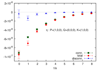
where we used smeared interpolators and for both the and the , respectively. is the local scalar current in position space. It can also be averaged over the spatial volume (multiplying by the phases ), to increase statistics. We detail the computation methods both for the connected and the disconnected contributions to the three-point functions in Appendix C. Fig. 8 shows the full three-point function and the contributions from connected and disconnected fermion loop diagrams. It is interesting to note that the magnitude of the disconnected contributions is large, especially for the decay to . Not surprisingly, the statistical error of the three-point function mainly comes from the disconnected part.

The three-point functions have the following spectral decomposition:
| (35) | ||||
where indicates the first excited states and we have neglected contributions from even higher excitations. is the amplitude of the state with , and . For brevity we suppress the momentum dependence of and . The first term on the r.h.s contains the ground state to ground state matrix element that we are interested in.
Note that the phase of the state is arbitrary and we choose it such that we have a real positive amplitude
| (36) |
This means that the matrix elements can be negative666 Charge conjugation invariance guarantees the matrix element is real in coordinate space, and then parity invariance gives a real three-point function in momentum space and, indeed, we obtained negative values for the . Since the sign of the matrix element is not physical, in the following we use its modulus.777Note, however, that relative signs are relevant for studies of flavour mixing angles in decays. This is similar to the connection of the sign of the distribution amplitude ratio to the sign of the respective mixing angle .
In order to determine the ground state to ground state matrix element reliably, it is important to take into account the excited state contributions to the three-point function. One way to do this is to use a large sink-source separation so that the excited state contributions are small. However, this is not possible in the current case because the statistical error grows rapidly (due to the disconnected terms), even for relatively small time separations. We need to employ an alternative approach.
First we obtain and by fitting the two-point function
| (37) |
using a functional form given by the first term, at sufficiently large . The energy gap, , is then determined by fitting the combination
| (38) |
to the form , where not only but also the amplitudes depend on the momentum . To extract the matrix element, , we compute the ratio
| (39) |
and use the fit function
| (40) |
where . Whenever the two-point function had a small overlap with the excited state and we were unable to extract , we only employed the first two terms of Eq. (40).
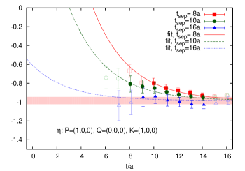
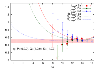
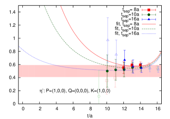
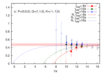
We generated three different data sets with and fitted these simultaneously. For the at the SU(3) flavour symmetric point, which has no disconnected contributions, we also generated data. For some momentum combinations only a subset of the available data was used in the fits, either due to the data being too noisy (for ) or because contributions from the second or higher excited states were significant (for ). Details of the chosen fit ranges are listed in Tables 9–12 of Appendix D and typical examples of the fits using Eq. (40) are shown in Fig. 9.
Again, we used correlated fits and varied the fit region to assess systematic uncertainties. The changes of the fit parameter values were found to be well within the statistical errors. The only exception was for the three-point function involving the meson at the SU(3) flavour symmetric point. In this case, the statistical errors were small such that the systematic uncertainties became relevant and we opted for employing an uncorrelated fit and a fit range that resulted in errors large enough to encompass the systematics.
IV.2 Results
The results for the form factor, derived from the matrix elements using Eq. (2), are listed in Tables 9–12 for the momentum ranges and in lattice units (). Note that we defined the four-momentum transfer as
| (41) |
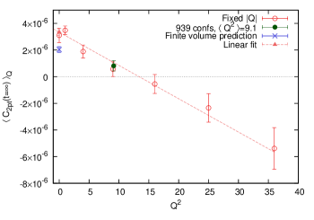
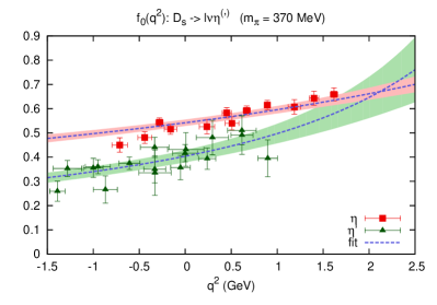
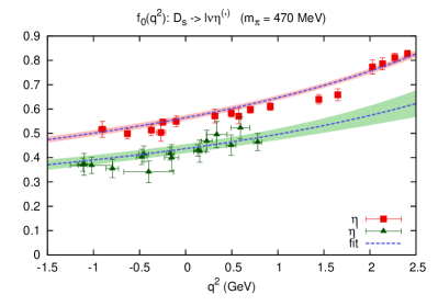
where the energies of the and states are listed in Tables 7 and 8 of Appendix D and depicted in Fig. 2. The values at non-zero momenta were determined directly, without using a dispersion relation. The dependence of on is shown in Fig. 10.
We used a one pole ansatz to interpolate the data to :
| (42) |
These curves are also shown in the figure. The resulting values for are listed in Table 5. The parameterization of Becirević and Kaidalov (BK) Becirević and Kaidalov (2000) is frequently used in the literature too. For the scalar form factor, this is essentially the same parameterization as Eq. (42) but the location of the pole is normalized with respect to the vector meson mass :888This should not be confused with the excited state of the pseudoscalar meson which we also denoted by a in the previous subsection.
| (43) |
with . The values of obtained from rescaling the parameter above are also listed in Table 5.
A comparison can be made with the values derived from light cone QCD sum rules (LCSRs) Offen et al. (2013), displayed in Table 5, where we assumed . Encouragingly, the results are broadly consistent. We find is larger for the than for the , independent of the quark mass, while for LCSRs the ordering cannot be resolved due to the large error for the . The ratios of the form factors are
| (44) |
A more detailed comparison would require an estimation of the dominant systematic uncertainties. These uncertainties are difficult to quantify in both studies, in the LCSRs case due to the approximations made, while in our study since we have a single lattice volume and lattice spacing. Considering our lightest pseudoscalar mass is around MeV and , extending the analysis to bigger volumes and smaller quark masses is important.
| Set | meson | |||
|---|---|---|---|---|
| S | 0.564(11) | 0.127(06) | 1.70(08) | |
| 0.437(18) | 0.119(23) | 1.81(35) | ||
| A | 0.542(13) | 0.090(14) | 2.35(36) | |
| 0.404(25) | 0.188(32) | 1.13(19) | ||
| LCSRs (at ) | 0.432(33) | — | — | |
| 0.520(80) | — | — |
IV.3 Outlook on phenomenology
The results given in the previous subsection do not allow for a direct determination of the widths and , since we computed rather than and used heavier-than-physical pion masses. Accordingly, a direct comparison to, for example, the ratio , as determined by the CLEO collaboration Yelton et al. (2009), is not yet possible. However, invoking some model assumptions, a tentative comparison can be made, albeit at the price of introducing an essentially unquantifiable uncertainty.
We calculate the ratio
| (45) |
where is the heavy-light kinematic factor
| (46) |
by replacing with the Ball-Zwicky ansatz Ball and Zwicky (2005)
| (47) |
and using a chirally extrapolated value of our lattice results for . are taken from the literature. We choose to compute the ratio rather than the individual decay rates since systematics in the chiral extrapolation and the phenomenological parameterisation of partially cancel between the decay rates for and .
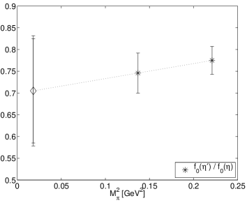
Using the above parameterisation only the ratio enters in Eq. (45); thus we extrapolate our two values for the ratio, given in Eq. (44), linearly in to the physical mass point, see Fig. 11; this yields , where the first uncertainty is statistical and the second one is systematic (taken as the difference between the central values at and ). For we take the experimental value Olive et al. (2014), and for , we use the central values determined in Ref. Offen et al. (2013), with 50% uncertainties: and .
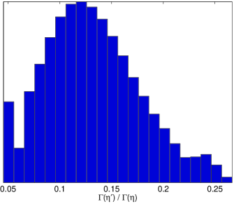
We vary and independently within the form factors and and evaluate Eq. (45) assuming Gaussian distributions of the five parameters , , , and within the respective errors given above. In the right panel of Fig. 11 the resulting histogram is shown. We find
| (48) |
which deviates by 1.6 from the CLEO result.
Taking these numbers at face value would be premature. We recall that we used both a chiral extrapolation (our computations were performed at and ) and a model for the form factors and . Our result, however, demonstrates the potential that a future lattice study of the form factors and will have. A study of these form factors, performed at the physical mass point, will significantly reduce the errors, which at present are dominated by systematics. We recall that the present work is mainly a pilot study to establish the feasibility of computations of form factors involving quark line disconnected diagrams.
V Conclusions and discussion
We calculated semileptonic decay form factors for and decays, by means of numerical lattice simulation. We included all disconnected fermion loop contributions. Despite the statistically noisy and computationally expensive disconnected part, we obtained the form factor at within statistical errors of less than 6%. The values at are and at and and at , where the errors are statistical only. The masses of the and the mesons are and at , and and at , keeping approximately constant. The mixing angle in the octet-singlet basis for the case is , and in the parameterization Eq. (29). There is no mixing in the flavour symmetric case. This means we have two different mixing angles, indicating higher Fock state contributions. We are not yet able to extrapolate the mixing angles, leading distribution amplitudes or masses to the physical point, however, assuming a monotonous dependence of the mixing angles on the light quark mass, their absolute values should increase towards the physical point.
It is interesting to note that the disconnected fermion loop contribution to is really significant. In Fig. 8 we saw that the relevant three-point function contains a large contribution from the disconnected diagram. This implies that the OZI suppressed gluonic contribution is not suppressed in this decay mode due to the chiral anomaly, as is also indicated by the fact that singlet and octet distribution amplitudes cannot be parameterized by a single angle, relative to the octet-singlet basis.
We calculated the scalar form factor which does not require knowledge of the renormalization constants. In order to compare with experiment, however, the vector form factor is more relevant, since, in the massless lepton limit, only contributes to the decay width. Technically, a computation of is of a similar level of complexity as the present study and we plan to pursue this in the near future. Finally, we remark that this work is an exploratory study and the quark masses we used are not yet physical. Having verified that computations of disconnected contributions to form factors are feasible, lighter pion masses and larger volumes will be simulated, also extending the present study to decays with the in the final state.
Acknowledgements.
We thank our collaborators within QCDSF who generated the ensembles analyzed here. We also thank the International Lattice DataGrid. We thank Vladimir Braun, Benjamin Gläßle, Meinulf Göckeler, Johannes Najjar and Paula Pérez-Rubio for their help, useful comments and discussions. This work was supported by the DFG (SFB/TRR 55) and the EU (ITN STRONGnet). The CHROMA software suite Edwards and Joó (2005) was used extensively along with the locally deflated domain decomposition solver implementation of openQCD http://luscher.web.cern.ch/luscher/openQCD/index.html . We benefited from time granted by PRACE (project 2012071240) on Fermi at CINECA, Bologna, as well as the Athene HPC and iDataCool clusters at the University of Regensburg. I. K. thanks the Ministry of Science and Technology in Taiwan (the grand 103-2811-M-009-014) and the hospitality of NCTS-north.Appendix A Details of the estimation of disconnected loops
In this Appendix we explain the methods implemented to calculate the disconnected loop given in Eq. (3). For convenience we restate the equation as
| (49) | ||||
| (50) |
The all-to-all propagator, , is computed using low mode deflation combined with stochastic estimation. This involves calculating (exact) low eigenmodes (in absolute magnitude) of the Hermitian Dirac operator :
| (51) |
where the are real. The low mode contribution to is given by
| (52) |
For small quark masses the low modes give the most singular directions of and the higher mode contributions become small. These higher modes are estimated stochastically using noise vectors, which approximately span a complete set
| (53) |
We have
| (54) |
where
| (55) |
is the source vector projected onto the subspace of the higher modes.
Stochastic estimation introduces additional (possibly dominant) noise on top of the gauge noise and this needs to be reduced. We implemented a number of techniques to achieve this:
-
1.
Time and spin partitioning Bernardson et al. (1993). The stochastic sources where given non-zero values only on every 4th timeslice and for a single spin index. To reconstruct the full propagator at every timeslice requires inversions.
-
2.
Hopping parameter acceleration (HPA) Thron et al. (1998). A Wilson-type Dirac operator
(56) satisfies the identity:
(57) for any integer . When this expression is inserted into Eq. (50) the first terms may be zero, where the value of depends on and the form of the Dirac operator. With stochastic estimation of these terms will only contribute to the noise and can be omitted, giving as an improved estimate of .
Combining this with low mode deflation we have
(58) For the clover action and we can use .
-
3.
The truncated solver method (TSM) Bali et al. (2010a). This method involves truncating the solver after a few iterations. The (hopefully small) correction to this truncation is calculated using a smaller number of stochastic estimates:
(59) where . The truncated part is calculated with a CG solver, while for we use the domain decomposition solver implementation of Ref. http://luscher.web.cern.ch/luscher/openQCD/index.html . To obtain the full expression for using HPA and low mode deflation one substitutes Eq. (59) into Eq. (58).
The parameters for the various techniques are chosen so that the stochastic error is minimized for fixed computational cost, see Ref. Bali et al. (2011a) for details. Our optimal choices are listed in Table 6. We found the HPA to be the most cost efficient noise reduction technique for our problem. The TSM only provided a slight improvement, due to the use of smeared loops. In general, the advantage of using the TSM will also depend on the efficiency of the solver.
Finally, we note that due to parity and charge conjugation considerations the disconnected loop in position space, , is real for . This means the imaginary part of our stochastic estimation of only contributes to the noise and we can set it to zero.
| Set | quark | TSM | ||
|---|---|---|---|---|
| S | , | truncated after 150 CG iterations | ||
| A | truncated after 120 CG iterations | |||
| (without TSM) |
Appendix B Two-point functions
In the octet-singlet basis, we need the following two-point functions:
| (60) | ||||
| (61) | ||||
| (62) | ||||
| (63) |
where is a connected two-point function of quark flavour and is the disconnected two-point function of quark flavours and :
| (64) |
where is the temporal lattice size, is the four-volume and is the disconnected fermion loop, Eq. (3), for quark flavour .
The calculation of is detailed in Appendix A. For the connected two-point function, we implemented low mode averaging (LMA) DeGrand and Schäfer (2004); Giusti et al. (2004) reusing the eigenmodes computed for the evaluation of the disconnected loop. As discussed in Ref. Bali et al. (2010b), LMA works very efficiently for pseudoscalar meson two-point functions. We used LMA for both the connected light-light () and strange-strange () two-point functions.
A connected two-point function with LMA is given by
| (65) |
where is the standard point-to-all two-point function, calculated with a single source point at . For simplicity, we have suppressed the quark flavour index and, initially, do not consider quark smearing. In Eq. (65), the low mode contribution to the point-to-all two-point function,
| (66) |
where and at the source and sink, is subtracted and replaced by the low mode contribution averaged over all lattice points:
| (67) |
Smearing the quarks is implemented by replacing the eigenvectors in Eq. (66) with smeared vectors, , for a smearing function .
Finally, we averaged over forward and backward propagating two-point functions, as well as rotationally equivalent momentum combinations.
Appendix C Three-point functions
The three-point function we need to determine is
| (68) |
where , are the interpolators, is the local scalar current and . The interpolators for and are obtained from Eq. (7), by solving the generalized eigenvalue problem for each . For , we used the improved mixing angles and as discussed in Sec. III.
We need both connected and disconnected contributions to calculate the three-point function Eq. (68), see Fig. 1. For the connected part, we used the stochastic method detailed in Ref. Evans et al. (2010). This approach allows us to access many momentum combinations at a lower computational cost compared to the standard sequential source method. We compute all rotationally equivalent momentum combinations average these.
The disconnected part is obtained from combining a connected charm-strange two-point function, , with a one-point quark loop of flavour :
| (69) |
and
| (70) |
Note that the charm-strange two-point function has a pseudoscalar source and a scalar sink. The one-point loop is calculated as described in Appendix A.
We employ low mode averaging in a similar way to that used for the computation of the connected two-point function in Appendix B, by averaging the low mode contributions to over :
| (71) |
where
| (72) |
and
| (73) |
The eigenvalues, , and eigenvectors, , are computed for the strange quark. We average over source points only, due to the computational cost of calculating the charm quark propagator, , for each source. We employ the subset with and with .
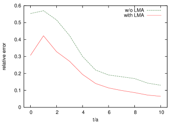
Finally, we averaged over rotationally equivalent momentum combinations, and averaged over and for each value of sink-source separation . Fig. 12 shows a typical example of a comparison of the relative error of the disconnected three-point function with and without low mode averaging. The figure illustrates that LMA reduces the error significantly.
Appendix D Data
The fitted values of two-point functions are listed in Tables 8 and 7. The values of the scalar form factor at each are listed in Tables 9, 10, 11 and 12.
| ground state | excited state | ||||||
| fit range | fit range | ||||||
| 12–24 | — | — | — | ||||
| 9–17 | — | — | — | ||||
| 8–17 | — | — | — | ||||
| 6–11 | — | — | — | ||||
| (lat. disp.)* | — | — | — | — | |||
| 6–24 | 2–4 | ||||||
| 9–23 | 2–7 | ||||||
| 8–14 | 2–4 | ||||||
| ** | 5–11 | — | — | — | |||
| (lat. disp.) | — | — | — | — | |||
| 7–11 | 2–4 | ||||||
| 6–11 | 2–4 | ||||||
| 6–10 | — | — | — | ||||
| ** | 4–7 | — | — | — | |||
| (lat. disp.) | — | — | — | — | |||
| 11–21 | 2–6 | ||||||
| 11–21 | 2–6 | ||||||
| 11–20 | 2–6 | ||||||
| 11–21 | 2–6 | ||||||
| 11–20 | 2–6 | ||||||
| 11–20 | 2–6 | ||||||
| (lat. disp.)* | — | — | — | — | |||
*: Not used.
**: Not included in the dispersion relation.
| ground state | excited state | ||||||
| fit range | fit range | ||||||
| 14–24 | 5–12 | ||||||
| 8–22 | 2–5 | ||||||
| 8–18 | 2–4 | ||||||
| 6–15 | 2–5 | ||||||
| ** | 4–10 | — | — | — | |||
| (lat. disp.)* | — | — | — | — | |||
| 4–11 | — | — | — | ||||
| 5–10 | — | — | — | ||||
| 6–12 | 2–4 | ||||||
| 8–12 | — | — | — | ||||
| (lat. disp.) | — | — | — | — | |||
| 11–24 | 2–7 | ||||||
| 12–24 | 2–7 | ||||||
| 12–24 | 2–8 | ||||||
| 10–24 | 2–8 | ||||||
| ** | 10–24 | 2–6 | |||||
| ** | 10–24 | 2–6 | |||||
| (lat. disp.)* | — | — | — | — | |||
*: Not used.
**: Not included in the dispersion relation.
| [fit range] | fit func. | equiv. | ||||
|---|---|---|---|---|---|---|
| , , | 8[2–6], 10[2–8], 16[9–14] | |||||
| , , | 8[2–6], 10[2–8], 16[9–14] | |||||
| , , | 8[2–6], 10[2–8], 16[9–14] | |||||
| , , | 8[2–6], 10[2–8], 16[9–14] | |||||
| , , | 8[2–6], 10[2–8], 16[10–14] | |||||
| , , | 8[2–6], 10[2–8], 16[9–14] | |||||
| , , | 8[2–6], 10[2–8], 16[9–14] | |||||
| , , | 8[3–6], 10[3–8], 16[10–14] | |||||
| , , | 8[3–6], 10[3–8], 16[10–14] | |||||
| , , | 8[3–6], 10[3–8], 16[10–14] | |||||
| , , | 8[3–6], 10[3–8], 16[11–14] | |||||
| , , | 8[3–6], 10[3–8], 16[11–14] |
| [fit range] | fit func. | equiv. | ||||
|---|---|---|---|---|---|---|
| , , | 8[2–6], 10[4–8], 16[10–14] | |||||
| , , | 8[4–6], 10[4–8], 16[12–14] | |||||
| , , | 8[2–6], 10[4–8], 16[10–14] | |||||
| , , | 8[2–6], 10[4–8], 16[10–14] | |||||
| , , | 8[2–6], 10[4–8], 16[11–12] | |||||
| , , | 8[2–6], 10[4–8], 16[11–13] | |||||
| , , | 8[3–5], 10[4–7], 16[10–13] | |||||
| , , | 8[3–5], 10[5–7], 16[10–13] | |||||
| , , | 8[3–5], 10[4–7], 16[10–13] | |||||
| , , | 8[4–5], 10[4–7], 16[11–13] | |||||
| , , | 8[3–4], 10[4–7], 16[10–13] | |||||
| , , | 8[3–5], 10[4–7], 16[10–13] | |||||
| , , | 8[4–5], 10[4–7], 16[12–13] | |||||
| , , | 8[4–5], 10[5–7], 16[11–13] | |||||
| , , | 8[4–5], 10[6–7], 16[11–13] | |||||
| , , | 8[4–5], 10[6–7], 16[12–13] | |||||
| , , | 8[4–5], 10[6–7], 16[12–13] |
| [fit range] | fit func. | equiv. | ||||
|---|---|---|---|---|---|---|
| , , | 16[7–10], 24[13–19] | |||||
| , , | 16[7–10], 24[13–19] | |||||
| , , | 16[8–11], 24[13–19] | |||||
| , , | 16[8–10], 24[13–19] | |||||
| , , | 8[4–5], 10[4–7], 16[4–13], 24[13–19] | |||||
| , , | 8[4–5], 10[4–7], 16[4–13], 24[12–19] | |||||
| , , | 8[4–5], 10[4–7], 16[4–13], 24[11–19] | |||||
| , , | 8[4–5], 10[4–7], 16[4–13], 24[15–20] | |||||
| , , | 8[4–5], 10[4–7], 16[4–13] | |||||
| , , | 8[4–5], 10[4–7], 16[4–13], 24[13–19] | |||||
| , , | 8[3–5], 10[3–7], 16[10–13], 24[18–21] | |||||
| , , | 8[3–5], 10[3–7], 16[8–13], 24[19–21] | |||||
| , , | 8[3–5], 10[3–7], 16[8–13], 24[17–21] | |||||
| , , | 8[3–5], 10[3–7], 16[8–13], 24[17–21] | |||||
| , , | 8[2–6], 10[2–8], 16[2–14], 24[13–21] | |||||
| , , | 8[2–6], 10[2–8], 16[10–14], 24[17–21] | |||||
| , , | 8[2–6], 10[2–8], 16[11–14] |
| [fit range] | fit func. | equiv. | ||||
|---|---|---|---|---|---|---|
| , , | 8[2–6], 10[4–8], 16[12–14] | |||||
| , , | 8[2–6], 10[4–8], 16[12–14] | |||||
| , , | 8[2–5], 10[3–7], 16[10–13] | |||||
| , , | 8[2–5], 10[3–7], 16[10–13] | |||||
| , , | 8[2–5], 10[3–7], 16[9–13] | |||||
| , , | 8[2–5], 10[3–7], 16[9–13] | |||||
| , , | 8[2–5], 10[3–7], 16[11–13] | |||||
| , , | 8[2–5], 10[3–7], 16[10–13] | |||||
| , , | 8[2–5], 10[3–7], 16[12–13] | |||||
| , , | 8[2–6], 10[4–8], 16[9–14] | |||||
| , , | 8[2–6], 10[4–8], 16[10–14] | |||||
| , , | 8[2–6], 10[4–8], 16[11–14] | |||||
| , , | 8[2–6], 10[4–8], 16[11–14] | |||||
| , , | 8[2–6], 10[4–8], 16[10–14] | |||||
| , , | 8[2–5], 10[5–7], 16[10–13] | |||||
| , , | 8[3–5], 10[5–7], 16[10–13] |
References
- Donald et al. (2014) G. Donald, C. Davies, J. Koponen, and G. Lepage (HPQCD), Phys.Rev. D90, 074506 (2014), arXiv:1311.6669 [hep-lat] .
- Colangelo and De Fazio (2001) P. Colangelo and F. De Fazio, Phys. Lett. B520, 78 (2001), arXiv:hep-ph/0107137 [hep-ph] .
- Azizi et al. (2011) K. Azizi, R. Khosravi, and F. Falahati, J. Phys. G38, 095001 (2011), arXiv:1011.6046 [hep-ph] .
- Offen et al. (2013) N. Offen, F. Porkert, and A. Schäfer, Phys. Rev. D88, 034023 (2013), arXiv:1307.2797 [hep-ph] .
- Di Donato et al. (2012) C. Di Donato, G. Ricciardi, and I. Bigi, Phys. Rev. D85, 013016 (2012), arXiv:1105.3557 [hep-ph] .
- Yelton et al. (2009) J. Yelton et al. (CLEO Collaboration), Phys.Rev. D80, 052007 (2009), arXiv:0903.0601 [hep-ex] .
- Kanamori (2012) I. Kanamori, PoS ConfinementX, 143 (2012), arXiv:1302.6087 [hep-lat] .
- Collins et al. (2013) S. Collins, I. Kanamori, and J. Najjar, eConf C130831 (2013), arXiv:1311.7393 [hep-lat] .
- Collins et al. (2014) S. Collins, I. Kanamori, and J. Najjar, PoS LATTICE2013, 392 (2014).
- Na et al. (2010) H. Na, C. T. Davies, E. Follana, G. P. Lepage, and J. Shigemitsu, Phys. Rev. D82, 114506 (2010), arXiv:1008.4562 [hep-lat] .
- Bali et al. (2011a) G. Bali et al. (QCDSF Collaboration), PoS LATTICE2011, 283 (2011a), arXiv:1111.4053 [hep-lat] .
- Bietenholz et al. (2010) W. Bietenholz, V. Bornyakov, N. Cundy, M. Göckeler, R. Horsley, et al., Phys. Lett. B690, 436 (2010), arXiv:1003.1114 [hep-lat] .
- Bietenholz et al. (2011) W. Bietenholz, V. Bornyakov, M. Göckeler, R. Horsley, W. Lockhart, et al., Phys. Rev. D84, 054509 (2011), arXiv:1102.5300 [hep-lat] .
- Cundy et al. (2009) N. Cundy, M. Göckeler, R. Horsley, T. Kaltenbrunner, A. Kennedy, et al., Phys. Rev. D79, 094507 (2009), arXiv:0901.3302 [hep-lat] .
- Sint and Weisz (1998) S. Sint and P. Weisz, Nucl. Phys. Proc. Suppl. 63, 856 (1998), arXiv:hep-lat/9709096 [hep-lat] .
- Bhattacharya et al. (2006) T. Bhattacharya, R. Gupta, W. Lee, S. R. Sharpe, and J. M. Wu, Phys. Rev. D73, 034504 (2006), arXiv:hep-lat/0511014 [hep-lat] .
- Borsanyi et al. (2012) S. Borsanyi, S. Durr, Z. Fodor, C. Hoelbling, S. D. Katz, et al., JHEP 1209, 010 (2012), arXiv:1203.4469 [hep-lat] .
- Horsley et al. (2013) R. Horsley, J. Najjar, Y. Nakamura, H. Perlt, D. Pleiter, et al., PoS LATTICE2013, 249 (2013), arXiv:1311.5010 [hep-lat] .
- Bali et al. (2011b) G. Bali, S. Collins, S. Durr, Z. Fodor, R. Horsley, et al., PoS LATTICE2011, 135 (2011b), arXiv:1108.6147 [hep-lat] .
- Güsken et al. (1989) S. Güsken, U. Löw, K. Mütter, R. Sommer, A. Patel, et al., Phys. Lett. B227, 266 (1989).
- Güsken (1990) S. Güsken, Nucl. Phys. B Proc. Suppl. 17, 361 (1990).
- Falcioni et al. (1985) M. Falcioni, M. Paciello, G. Parisi, and B. Taglienti, Nucl. Phys. B251, 624 (1985).
- DeGrand and Schäfer (2004) T. A. DeGrand and S. Schäfer, Comput. Phys. Commun. 159, 185 (2004), arXiv:hep-lat/0401011 [hep-lat] .
- Giusti et al. (2004) L. Giusti, P. Hernandez, M. Laine, P. Weisz, and H. Wittig, JHEP 0404, 013 (2004), arXiv:hep-lat/0402002 [hep-lat] .
- Christ et al. (2010) N. Christ, C. Dawson, T. Izubuchi, C. Jung, Q. Liu, et al., Phys. Rev. Lett. 105, 241601 (2010), arXiv:1002.2999 [hep-lat] .
- Gregory et al. (2012) E. B. Gregory, A. C. Irving, C. M. Richards, and C. McNeile (UKQCD Collaboration), Phys. Rev. D86, 014504 (2012), arXiv:1112.4384 [hep-lat] .
- Dudek et al. (2011) J. J. Dudek, R. G. Edwards, B. Joo, M. J. Peardon, D. G. Richards, et al., Phys. Rev. D83, 111502 (2011), arXiv:1102.4299 [hep-lat] .
- Michael et al. (2013) C. Michael, K. Ottnad, and C. Urbach, Phys. Rev. Lett. 111, 181602 (2013), arXiv:1310.1207 [hep-lat] .
- Olive et al. (2014) K. Olive et al. (Particle Data Group), Chin.Phys. C38, 090001 (2014).
- Aoki et al. (2007) S. Aoki, H. Fukaya, S. Hashimoto, and T. Onogi, Phys. Rev. D76, 054508 (2007), arXiv:0707.0396 [hep-lat] .
- Bilson-Thompson et al. (2003) S. O. Bilson-Thompson, D. B. Leinweber, and A. G. Williams, Annals Phys. 304, 1 (2003), arXiv:hep-lat/0203008 [hep-lat] .
- Morningstar and Peardon (2004) C. Morningstar and M. J. Peardon, Phys. Rev. D69, 054501 (2004), arXiv:hep-lat/0311018 [hep-lat] .
- Bali et al. (2001) G. S. Bali et al. (SESAM Collaboration, TL Collaboration), Phys. Rev. D64, 054502 (2001), arXiv:hep-lat/0102002 [hep-lat] .
- Brower et al. (2003) R. Brower, S. Chandrasekharan, J. W. Negele, and U. Wiese, Phys. Lett. B560, 64 (2003), arXiv:hep-lat/0302005 [hep-lat] .
- Kaneko et al. (2009) T. Kaneko et al. (TWQCD collaboration, JLQCD Collaboration), PoS LAT2009, 107 (2009), arXiv:0910.4648 [hep-lat] .
- Feldmann (2000) T. Feldmann, Int. J. Mod. Phys. A15, 159 (2000), arXiv:hep-ph/9907491 [hep-ph] .
- Becirević and Kaidalov (2000) D. Becirević and A. B. Kaidalov, Phys. Lett. B478, 417 (2000), arXiv:hep-ph/9904490 [hep-ph] .
- Ball and Zwicky (2005) P. Ball and R. Zwicky, Phys.Rev. D71, 014015 (2005), arXiv:hep-ph/0406232 [hep-ph] .
- Edwards and Joó (2005) R. G. Edwards and B. Joó (SciDAC Collaboration, LHPC Collaboration, UKQCD Collaboration), Nucl. Phys. Proc. Suppl. 140, 832 (2005), arXiv:hep-lat/0409003 [hep-lat] .
- (40) http://luscher.web.cern.ch/luscher/openQCD/index.html, .
- Bernardson et al. (1993) S. Bernardson, P. McCarty, and C. Thron, Comput. Phys. Commun. 78, 256 (1993).
- Thron et al. (1998) C. Thron, S. Dong, K. Liu, and H. Ying, Phys. Rev. D57, 1642 (1998), arXiv:hep-lat/9707001 [hep-lat] .
- Bali et al. (2010a) G. S. Bali, S. Collins, and A. Schäfer, Comput. Phys. Commun. 181, 1570 (2010a), arXiv:0910.3970 [hep-lat] .
- Bali et al. (2010b) G. Bali, L. Castagnini, and S. Collins, PoS LATTICE2010, 096 (2010b), arXiv:1011.1353 [hep-lat] .
- Evans et al. (2010) R. Evans, G. Bali, and S. Collins, Phys. Rev. D82, 094501 (2010), arXiv:1008.3293 [hep-lat] .