Playing with Duality: An Overview of Recent Primal-Dual Approaches for Solving Large-Scale Optimization Problems

Abstract

Optimization methods are at the core of many problems in signal/image processing, computer vision, and machine learning. For a long time, it has been recognized that looking at the dual of an optimization problem may drastically simplify its solution. Deriving efficient strategies which jointly brings into play the primal and the dual problems is however a more recent idea which has generated many important new contributions in the last years. These novel developments are grounded on recent advances in convex analysis, discrete optimization, parallel processing, and nonsmooth optimization with emphasis on sparsity issues. In this paper, we aim at presenting the principles of primal-dual approaches, while giving an overview of numerical methods which have been proposed in different contexts. We show the benefits which can be drawn from primal-dual algorithms both for solving large-scale convex optimization problems and discrete ones, and we provide various application examples to illustrate their usefulness.

I Motivation and importance of the topic

Optimization [1] is an extremely popular paradigm which constitutes the backbone of many branches of applied mathematics and engineeering, such as signal processing, computer vision, machine learning, inverse problems, and network communications, to mention just a few. The popularity of optimization approaches often stems from the fact that many problems from the above fields are typically characterized by a lack of closed form solutions and by uncertainties. In signal and image processing, for instance, uncertainties can be introduced due to noise, sensor imperfectness, or ambiguities that are often inherent in the visual interpretation. As a result, perfect or exact solutions hardly exist, whereas inexact but optimal (in a statistical or an application-specific sense) solutions and their efficient computation is what one aims at. At the same time, one important characteristic that is nowadays shared by increasingly many optimization problems encountered in the above areas is the fact that these problems are often of very large scale. A good example is the field of computer vision where one often needs to solve low level problems that require associating at least one (and typically more than one) variable to each pixel of an image (or even worse of an image sequence as in the case of video) [2]. This leads to problems that easily can contain millions of variables, which are therefore the norm rather than the exception in this context.

Similarly, in fields like machine learning [3, 4], due to the great ease with which data can now be collected and stored, quite often one has to cope with truly massive datasets and to train very large models, which thus naturally lead to optimization problems of very high dimensionality [5]. Of course, a similar situation arises in many other scientific domains, including application areas such as inverse problems (e.g., medical image reconstruction or satellite image restoration) or telecommunications (e.g., network design, network provisioning) and industrial engineering. Due to this fact, computational efficiency constitutes a major issue that needs to be thoroughly addressed. This, therefore, makes mandatory the use of tractable optimization techniques that are able to properly exploit the problem structures, but which at the same time remain applicable to a class of problems as wide as possible.

A bunch of important advances that took place in this regard over the last years concerns a particular class of optimization approaches known as primal-dual methods. As their name implies, these approaches proceed by concurrently solving a primal problem (corresponding to the original optimization task) as well as a dual formulation of this problem. As it turns out, in doing so they are able to exploit more efficiently the problem specific properties, thus offering in many cases important computational advantages, some of which are briefly mentioned next for two very broad classes of problems.

I-1 Convex optimization

Primal-dual methods have been primarily employed in convex optimization problems [6, 7, 8] where strong duality holds. They have been successfully applied to various types of nonlinear and nonsmooth cost functions that are prevalent in the above-mentioned application fields.

Many such applied problems can essentially be expressed under the form of a minimization of a sum of terms, where each term is given by the composition of a convex function with a linear operator. One first advantage of primal-dual methods pertains to the fact that they can yield very efficient splitting optimization schemes, according to which a solution to the original problem is iteratively computed through solving a sequence of easier subproblems, each one involving only one of the terms appearing in the objective function.

The resulting primal-dual splitting schemes can also handle both differentiable and nondifferentiable terms, the former by use of gradient operators (i.e., through explicit steps) and the latter by use of proximity operators (i.e., through implicit steps) [9, 10]. Depending on the target functions, either explicit or implicit steps may be easier to implement. Therefore, the derived optimization schemes exploit the properties of the input problem, in a flexible manner, thus leading to very efficient first-order algorithms.

Even more importantly, primal-dual techniques are able to achieve what is known as full splitting in the optimization literature, meaning that each of the operators involved in the problem (i.e., not only the gradient or proximity operators but also the involved linear operators) is used separately [11]. As a result, no call to the inversion of a linear operator, which is an expensive operation for large scale problems, is required during the optimization process. This is an important feature which gives these methods a significant computational advantage compared with all other splitting-based approaches.

Last but not least, primal-dual methods lead to algorithms that are easily parallelizable, which is nowadays becoming increasingly important for efficiently handling high-dimensional problems.

I-2 Discrete optimization

Besides convex optimization, another important area where primal-dual methods play a prominent role is discrete optimization. This is of particular significance given that a large variety of tasks from signal processing, computer vision, and pattern recognition are formulated as discrete labeling problems, where one seeks to optimize some measure related to the quality of the labeling [12]. This includes, for instance, tasks such as image segmentation, optical flow estimation, image denoising, stereo matching, to mention a few examples from image analysis. The resulting discrete optimization problems not only are of very large size, but also typically exhibit highly nonconvex objective functions, which are generally intricate to optimize.

Similarly to the case of convex optimization, primal-dual methods again offer many computational advantages, leading often to very fast graph-cut or message-passing-based algorithms, which are also easily parallelizable, thus providing in many cases a very efficient way for handling discrete optimization problems that are encountered in practice [13, 14, 15, 16]. Besides being efficient, they are also successful in making little compromises regarding the quality of the estimated solutions. Techniques like the so-called primal-dual schema are known to provide a principled way for deriving powerful approximation algorithms to difficult combinatorial problems, thus allowing primal-dual methods to often exhibit theoretical (i.e., worst-case) approximation properties. Furthermore, apart from the aforementioned worst-case guaranties, primal-dual algorithms can also provide (for free) per-instance approximation guaranties. This is essentially made possible by the fact that these methods are estimating not only primal but also dual solutions.

Convex optimization and discrete optimization have different background theory originally. Convex optimization may appear as the most tractable topic in optimization, for which many efficient algorithms have been developed allowing a broad class of problems to be solved. By contrast, combinatorial optimization problems are generally NP-hard. However, many convex relaxations of certain discrete problems can provide good approximate solutions to the original ones [17, 18]. The problems encountered in discrete optimization therefore constitute a source of inspiration for developing novel convex optimization techniques.

Goals of this tutorial paper. Based on the above observations, our objectives will be the following:

1. To provide a thorough introduction that intuitively explains the basic principles and ideas behind primal-dual approaches.

2. To describe how these methods can be employed both in the context of continuous optimization and in the context of discrete optimization.

3. To explain some of the recent advances that have taken place concerning primal-dual algorithms for solving large-scale optimization problems.

4. To detail useful connections between primal-dual methods and some widely used optimization techniques like the alternating direction method of multipliers (ADMM) [19, 20].

5. Finally, to provide examples of useful applications in the context of image analysis and signal processing.

The remainder of the paper is structured as follows. In Section II, we introduce the necessary methodological background on optimization. Our presentation is grounded on the powerful notion of duality known as Fenchel’s duality, from which duality properties in linear programming can be deduced. We also introduce useful tools from functional analysis and convex optimization, including the notions of subgradient and subdifferential, conjugate function, and proximity operator. The following two sections explain and describe various primal-dual methods. Section III is devoted to convex optimization problems. We discuss the merits of various algorithms and explain their connections with ADMM, that we show to be a special case of primal-dual proximal method. Section IV deals with primal-dual methods for discrete optimization. We explain how to derive algorithms of this type based on the primal-dual schema which is a well-known approximation technique in combinatorial optimization, and we also present primal-dual methods based on LP relaxations and dual decomposition. In Section V, we present applications from the domains of signal processing and image analysis, including inverse problems and computer vision tasks related to Markov Random Field energy minimization. In Section VI, we finally conclude the tutorial with a brief summary and discussion.

II Optimization background

In this section, we introduce the necessary mathematical definitions and concepts used for introducing primal-dual algorithms in later sections. Although the following framework holds for general Hilbert spaces, for simplicity we will focus on the finite dimensional case.

II-A Notation

In this paper, we will consider functions from $\mathbb{R}^{N}$ to $\,\left]-\infty,+\infty\right]$. The fact that we allow functions to take $+\infty$ value is useful in modern optimization to discard some “forbidden part” of the space when searching for an optimal solution (for example, in image processing problems, the components of the solution often are intensity values which must be nonnegative). The domain of a function $f\colon\mathbb{R}^{N}\to\,\left]-\infty,+\infty\right]$ is the subset of $\mathbb{R}^{N}$ where this function takes finite values, i.e. $\mathrm{dom}\,f=\big{\{}{x\in\mathbb{R}^{N}}~{}\big{|}~{}{f(x)<+\infty}\big{\}}$. A function with a nonempty domain is said to be proper. A function $f$ is convex if

$$\big{(}\forall(x,y)\in(\mathbb{R}^{N})^{2}\big{)}(\forall\lambda\in[0,1])\qquad f(\lambda x+(1-\lambda)y)\leq\lambda f(x)+(1-\lambda)f(y).$$ (1)

The class of functions for which most of the main results in convex analysis have been established is $\Gamma_{0}(\mathbb{R}^{N})$, the class of proper, convex, lower-semicontinuous functions from $\mathbb{R}^{N}$ to $\,\left]-\infty,+\infty\right]$. Recall that a function $f\colon\mathbb{R}^{N}\to\,\left]-\infty,+\infty\right]$ is lower-semicontinuous if its epigraph $\operatorname{epi}f=\big{\{}{(x,\zeta)\in\mathrm{dom}\,f\times\mathbb{R}}~{}\big{|}~{}{f(x)\leq\zeta}\big{\}}$ is a closed set (see Fig. 1).

Figure 1: Illustration of the lower-semicontinuity property.

If $C$ is a nonempty subset of $\mathbb{R}^{N}$, the indicator function of $C$ is defined as

$$(\forall x\in\mathbb{R}^{N})\qquad\iota_{C}(x)=\begin{cases}0&\mbox{if $x\in C$}\\ +\infty&\mbox{otherwise.}\end{cases}$$ (2)

This function belongs to $\Gamma_{0}(\mathbb{R}^{N})$ if and only if $C$ is a nonempty closed convex set.

The Moreau subdifferential of a function $f\colon\mathbb{R}^{N}\to\,\left]-\infty,+\infty\right]$ at $x\in\mathbb{R}^{N}$ is defined as

$$\partial f(x)=\big{\{}{u\in\mathbb{R}^{N}}~{}\big{|}~{}{(\forall y\in\mathbb{R}^{N})\;\;f(y)\geq f(x)+{u}^{\!\top}{(y-x)}}\big{\}}.$$ (3)

Any vector $u$ in $\partial f(x)$ is called a subgradient of $f$ at $x$ (see Fig. 2).

Figure 2: Examples of subgradients $u$ of a function $f$ at $x$.

Fermat’s rule states that $0$ is a subgradient of $f$ at $x$ if and only if $x$ belongs to the set of global minimizers of $f$. If $f$ is a proper convex function which is differentiable at $x$, then its subdifferential at $x$ reduces to the singleton consisting of its gradient, i.e. $\partial f(x)=\{\nabla f(x)\}$. Note that, in the nonconvex case, extended definitions of the subdifferential may be useful such as the limiting subdifferential [21], but this one reduces to the Moreau subdifferential when the function is convex.

II-B Proximity operator

A concept which has been of growing importance in recent developments in optimization is the concept of proximity operator. It must be pointed out that the proximity operator was introduced in the early work by J. J. Moreau (1923-2014) [9]. The proximity operator of a function $f\in\Gamma_{0}(\mathbb{R}^{N})$ is defined as

$$\mathrm{prox}_{f}\colon\mathbb{R}^{N}\to\mathbb{R}^{N}\colon x\mapsto\underset{\begin{subarray}{c}{y\in\mathbb{R}^{N}}\end{subarray}}{\mathrm{argmin}}\;\;f(y)+\frac{1}{2}\|y-x\|^{2}$$ (4)

where $\|\cdot\|$ denotes the Euclidean norm. For every $x\in\mathbb{R}^{N}$, $\mathrm{prox}_{f}x$ can thus be interpreted as the result of a regularized minimization of $f$ in the neighborhood of $x$. Note that the minimization to be performed to calculate $\mathrm{prox}_{f}x$ always has a unique solution. Fig. 3 shows the variations of the $\mathrm{prox}_{f}$ function when $f\colon\mathbb{R}\to\mathbb{R}\colon x\mapsto|x|^{p}$ with $p\geq 1$. In the case when $p=1$, the classical soft-thesholding operation is obtained.

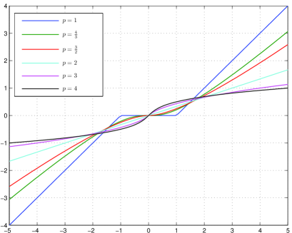
Figure 3: Graph of $\mathrm{prox}_{|\cdot|^{p}}$. This power $p$ function is often used to regularize inverse problems.

In the case when $f$ is equal to the indicator function of a nonempty closed convex set $C\subset\mathbb{R}^{N}$, the proximity operator of $f$ reduces to the projection $P_{C}$ onto this set, i.e. $(\forall x\in\mathbb{R}^{N})$ $P_{C}x=\underset{\begin{subarray}{c}{y\in C}\end{subarray}}{\mathrm{argmin}}\;\;\|y-x\|$.

This shows that proximity operators can be viewed as extensions of projections onto convex sets. The proximity operator enjoys many properties of the projection, in particular it is firmly nonexpansive. The firm nonexpansiveness can be viewed as a generalization of the strict contraction property which is the engine behind the Banach-Picard fixed point theorem. This property makes the proximity operator successful in ensuring the convergence of fixed point algorithms grounded on its use. For more details about proximity operators and their rich properties, the reader is refered to the tutorial papers in [10, 5, 22]. The definition of the proximity operator can be extended to nonconvex lower-semicontinuous functions which are lower bounded by an affine function, but $\mathrm{prox}_{f}x$ is no longer guaranteed to be uniquely defined at any given point $x$.

II-C Conjugate function

A fundamental notion when dealing with duality issues is the notion of conjugate function. The conjugate of a function $f\colon\mathbb{R}^{N}\to\,\left]-\infty,+\infty\right]$ is the function $f^{*}$ defined as

$$f^{*}\colon\mathbb{R}^{N}\to\,\left]-\infty,+\infty\right]\colon u\mapsto\sup_{x\in\mathbb{R}^{N}}\big{(}{x}^{\!\top}{u}-f(x)\big{)}.$$ (5)

This concept was introduced by A. M. Legendre (1752-1833) in the one-variable case, and it was generalized by M. W. Fenchel (1905-1988). A graphical illustration of the conjugate function is provided in Fig. 4. In particular, for every vector $x\in\mathbb{R}^{N}$ such that the supremum in (5) is attained, $u$ is a subgradient of $f$ at $x$.

Figure 4: Graphical interpretation of the conjugate function.

It must be emphasized that, even if $f$ is nonconvex, $f^{*}$ is a (non necessarily proper) lower-semicontinuous convex function. In addition, when $f\in\Gamma_{0}(\mathbb{R}^{N})$, then $f^{*}\in\Gamma_{0}(\mathbb{R}^{N})$, and also the biconjugate of $f$ (that is the conjugate of its conjugate) is equal to $f$. This means that we can express any function $f$ in $\Gamma_{0}(\mathbb{R}^{N})$ as

$$(\forall x\in\mathbb{R}^{N})\qquad f(x)=\sup_{u\in\mathbb{R}^{N}}\big{(}{u}^{\!\top}{x}-f^{*}(u)\big{)}.$$ (6)

A geometrical interpretation of this result is that the epigraph of any proper lower-semicontinuous convex function always is an intersection of closed half-spaces.

As we have seen, the subdifferential plays an important role in the characterization of the minimizers of a function. A natural question is thus to enquire about the relations existing between the subdifferential of a function $f\colon\mathbb{R}^{N}\to\,\left]-\infty,+\infty\right]$ and the subdifferential of its conjugate function. An answer is provided by the following important properties:

$$u\in\partial f(x)\quad \Rightarrow\quad x\in\partial f^{*}(u)\qquad\mbox{if $f$ is proper}$$

$$u\in\partial f(x)\quad \Leftrightarrow\quad x\in\partial f^{*}(u)\qquad\mbox{if $f\in\Gamma_{0}(\mathbb{R}^{N})$.}$$ (7)

Another important property is Moreau’s decomposition formula which links the proximity operator of a function $f\in\Gamma_{0}(\mathbb{R}^{N})$ to the proximity operator of its conjugate:

$$(\forall x\in\mathbb{R}^{N})(\forall\gamma\in\,\left]0,+\infty\right[)\qquad x=\mathrm{prox}_{\gamma f}x+\gamma\,\mathrm{prox}_{\gamma^{-1}f^{*}}(\gamma^{-1}x).$$ (8)

Other useful properties of the conjugation operation are listed in Table I, where a parallel is drawn with the multidimensional Fourier transform, which is a more familiar tool in signal and image processing. Conjugation also makes it possible to build an insightful bridge between the main two kinds of nonsmooth convex functions encountered in signal and image processing problems, namely indicator functions of feasibility constraints and sparsity measures (see framebox below.

TABLE I: Parallelism between properties of the Legendre-Fenchel conjugation [10] and of the Fourier transform. $f$ is a function defined on $\mathbb{R}^{N}$, $f^{*}$ denotes its conjugate, $\widehat{f}$ is its Fourier transform such that $\widehat{f}(\nu)=\int_{\mathbb{R}^{N}}f(x)\exp(-\jmath 2\pi{x}^{\!\top}{\nu})dx$ where $\nu\in\mathbb{R}^{N}$ and $\jmath$ is the imaginary unit (a similar notation is used for other functions), $h$, $g$, and $(f_{m})_{1\leq m\leq M}$ are functions defined on $\mathbb{R}^{N}$, $(\varphi_{j})_{1\leq j\leq N}$ are functions defined on $\mathbb{R}$, $\psi$ is an even function defined on $\mathbb{R}$, $\widetilde{\psi}$ is defined as $\widetilde{\psi}(\rho)=2\pi\rho^{(2-N)/2}\int_{0}^{+\infty}r^{N/2}J_{(N-2)/2}(2\pi r\rho)\psi(r)dr$ where $\rho\in\mathbb{R}$ and $J_{(N-2)/2}$ is the Bessel function of order $(N-2)/2$, and $\delta$ denotes the Dirac distribution. (Some properties of the Fourier transform may require some technical assumptions.)

		conjugation		Fourier transform
	Property	$h(x)$	$h^{*}(u)$	$h(x)$	$\widehat{h}(\nu)$
i	invariant function	$\frac{1}{2}\|x\|^{2}$	$\frac{1}{2}\|u\|^{2}$	$\exp(-\pi\|x\|^{2})$	$\exp(-\pi\|\nu\|^{2})$
ii	translation	$f(x-c)$	$f^{*}(u)+{c}^{\!\top}{u}$	$f(x-c)$	$\exp(-\jmath 2\pi{c}^{\!\top}{\nu})\widehat{f}(\nu)$
	$c\in\mathbb{R}^{N}$
iii	dual translation	$f(x)+{c}^{\!\top}{x}$	$f^{*}(u-c)$	$\exp(\jmath 2\pi{c}^{\!\top}{x})f(x-c)$	$\widehat{f}(\nu-c)$
	$c\in\mathbb{R}^{N}$
iv	scalar multiplication	$\alpha f(x)$	$\alpha f^{*}\left(\frac{u}{\alpha}\right)$	$\alpha f(x)$	$\alpha\widehat{f}(\nu)$
	$\alpha\in\,\left]0,+\infty\right[$
v	invertible linear transform	$f(Lx)$	$f^{*}\big{(}(L^{-1})^{\top}u\big{)}$	$f(Lx)$	$\frac{1}{|\operatorname{det}(L)|}\widehat{f}\big{(}(L^{-1})^{\top}\nu\big{)}$
	$L\in\mathbb{R}^{N\times N}$ invertible
vi	scaling	$f\left(\frac{x}{\alpha}\right)$	$f^{*}(\alpha u)$	$f\left(\frac{x}{\alpha}\right)$	$|\alpha|\widehat{f}(\alpha\nu)$
	$\alpha\in\mathbb{R}^{*}$
vii	reflection	$f(-x)$	$f^{*}(-u)$	$f(-x)$	$\widehat{f}(-\nu)$
viii	separability	$\displaystyle\sum_{j=1}^{N}\varphi_{j}(x^{(j)})$	$\displaystyle\sum_{j=1}^{N}\varphi_{j}^{*}(u^{(j)})$	$\displaystyle\prod_{j=1}^{N}\varphi_{j}(x^{(j)})$	$\displaystyle\prod_{j=1}^{N}\widehat{\varphi}_{j}(\nu^{(j)})$
		$x=(x^{(j)})_{1\leq j\leq N}$	$u=(u^{(j)})_{1\leq j\leq N}$	$x=(x^{(j)})_{1\leq j\leq N}$	$\nu=(\nu^{(j)})_{1\leq j\leq N}$
ix	isotropy	$\psi(\|x\|)$	$\psi^{*}(\|u\|)$	$\psi(\|x\|)$	$\widetilde{\psi}(\|\nu\|)$
x	inf-convolution	$(f\mbox{\footnotesize$\,\square\,$}g)(x)$	$f^{*}(u)+g^{*}(u)$	$(f\star g)(x)$	$\widehat{f}(\nu)\widehat{g}(\nu)$
	/convolution	$\displaystyle=\inf_{y\in\mathbb{R}^{N}}f(y)+g(x-y)$		$\displaystyle=\int_{\mathbb{R}^{N}}f(y)g(x-y)dy$
xi	sum/product	$f(x)+g(x)$	$(f^{*}\mbox{\footnotesize$\,\square\,$}g^{*})(u)$	$f(x)g(x)$	$(\widehat{f}\star\widehat{g})(\nu)$
		$f\in\Gamma_{0}(\mathbb{R}^{N})$, $g\in\Gamma_{0}(\mathbb{R}^{N})$
		$\mathrm{dom}\,f\cap\mathrm{int}\,(\mathrm{dom}\,g)\neq\varnothing$
xii	identity element	$\iota_{\{0\}}(x)$	$0$	$\delta(x)$	$1$
	of convolution
xiii	identity element	$0$	$\iota_{\{0\}}(u)$	$1$	$\delta(\nu)$
	of addition/product
xiv	offset	$f(x)+\alpha$	$f^{*}(u)-\alpha$	$f(x)+\alpha$	$\widehat{f}(\nu)+\alpha\delta(\nu)$
	$\alpha\in\mathbb{R}$
xv	infinum/sum	$\displaystyle\inf_{1\leq m\leq M}f_{m}(x)$	$\displaystyle\sup_{1\leq m\leq M}f_{m}^{*}(u)$	$\displaystyle\sum_{m=1}^{M}f_{m}(x)$	$\displaystyle\sum_{m=1}^{M}\widehat{f}_{m}(\nu)$
xvi	value at $0$	$f^{*}(0)=-\inf f$		$\displaystyle\widehat{f}(0)=\int_{\mathbb{R}^{N}}f(x)dx$

CONJUGATES OF SUPPORT FUNCTIONS The support function of a set $C\subset\mathbb{R}^{N}$ is defined as $$(\forall u\in\mathbb{R}^{N})\qquad\sigma_{C}(u)=\sup_{x\in C}{x}^{\!\top}{u}.$$ (9) In fact, a function $f$ is the support function of a nonempty closed convex set $C$ if and only if it belongs to $\Gamma_{0}(\mathbb{R}^{N})$ and it is positively homogeneous [8], i.e. $$(\forall x\in\mathbb{R}^{N})(\forall\alpha\in\,\left]0,+\infty\right[)\qquad f(\alpha x)=\alpha f(x).$$ Examples of such functions are norms, e.g. the $\ell_{1}$-norm: $$\big{(}\forall x=(x^{(j)})_{1\leq j\leq N}\in\mathbb{R}^{N}\big{)}\qquad f(x)=\|x\|_{1}=\sum_{j=1}^{N}|x^{(j)}|$$ which is a useful convex sparsity-promoting measure in LASSO estimation [23] and in compressive sensing [24]. Another famous example is the Total Variation semi-norm [25] which is popular in image processing for retrieving constant areas with sharp contours. An important property is that, if $C$ is a nonempty closed convex set, the conjugate of its support function is the indicator function of $C$. For example, the conjugate function of the $\ell_{1}$-norm is the indicator function of the hypercube $[-1,1]^{N}$. This shows that using sparsity measures are equivalent in the dual domain to imposing some constraints. .

II-D Duality results

A wide array of problems in signal and image processing can be expressed under the following variational form:

$$\underset{\begin{subarray}{c}{x\in\mathbb{R}^{N}}\end{subarray}}{\mathrm{minimize}}\;\;f(x)+g(Lx)$$ (10)

where $f\colon\mathbb{R}^{N}\to\,\left]-\infty,+\infty\right]$, $g\colon\mathbb{R}^{K}\to\,\left]-\infty,+\infty\right]$, and $L\in\mathbb{R}^{K\times N}$. Problem (10) is usually referred to as the primal problem which is associated with the following dual problem [6, 26, 8]:

$$\underset{\begin{subarray}{c}{v\in\mathbb{R}^{K}}\end{subarray}}{\mathrm{minimize}}\;\;f^{*}(-L^{\top}v)+g^{*}(v).$$ (11)

The latter problem may be easier to solve than the former one, especially when $K$ is much smaller than $N$.

A question however is to know whether solving the dual problem may bring some information on the solution of the primal one. A first answer to this question is given by the Fenchel-Rockafellar duality theorem which basically states that solving the dual problem provides a lower bound on the minimum value which can be obtained in the primal one. More precisely, if $f$ and $g$ are proper functions and if $\mu$ and $\mu^{*}$ denote the infima of the functions minimized in the primal and dual problems, respectively, then weak duality holds, which means that $\mu\geq-\mu^{*}$. If $\mu$ is finite, $\mu+\mu^{*}$ is called the duality gap. In addition, if $f\in\Gamma_{0}(\mathbb{R}^{N})$ and $g\in\Gamma_{0}(\mathbb{R}^{K})$, then, under appropriate qualification conditions, there always exists a solution to the dual problem and the duality gap vanishes. When the duality gap is equal to zero, it is said that strong duality holds.

CONSENSUS AND SHARING ARE DUAL PROBLEMS Suppose that our objective is to minimize a composite function $\sum_{m=1}^{M}g_{m}$ where the potential $g_{m}\colon\mathbb{R}^{N}\to\,\left]-\infty,+\infty\right]$ is computed at the vertex of index $m\in\{1,\ldots,M\}$ of a graph. A classical technique to perform this task in a distributed or parallel manner [20] consists of reformulating this problem as a consensus problem, where a variable is assigned to each vertex, and the defined variables $x_{1},\ldots,x_{M}$ are updated so as to reach a consensus: $x_{1}=\ldots=x_{M}$. This means that, in the product space $(\mathbb{R}^{N})^{M}$ the original optimization problem can be rewritten as $$\underset{\begin{subarray}{c}{\boldsymbol{x}=(x_{1},\ldots,x_{M})\in(\mathbb{R}^{N})^{M}}\end{subarray}}{\mathrm{minimize}}\;\;\iota_{D}(\boldsymbol{x})+\underbrace{\sum_{m=1}^{M}g_{m}(x_{m})}_{\mbox{$g(\boldsymbol{x})$}}$$ where $D$ is the vector space defined as $D=\big{\{}{\boldsymbol{x}=(x_{1},\ldots,x_{M})\in(\mathbb{R}^{N})^{M}}~{}\big{|}~{}{x_{1}=\ldots=x_{M}}\big{\}}$. By noticing that the conjugate of the indicator function of a vector space is the indicator function of its orthogonal complement, it is easy to see that the dual of this consensus problem has the following form: $$\underset{\begin{subarray}{c}{\boldsymbol{v}=(v_{1},\ldots,v_{M})\in(\mathbb{R}^{N})^{M}}\end{subarray}}{\mathrm{minimize}}\;\;\iota_{D^{\bot}}(\boldsymbol{v})+\underbrace{\sum_{m=1}^{M}g_{m}^{*}(v_{m})}_{\mbox{$g^{*}(\boldsymbol{v})$}}$$ where $D^{\bot}=\big{\{}{\boldsymbol{v}=(v_{1},\ldots,v_{M})\in(\mathbb{R}^{N})^{M}}~{}\big{|}~{}{v_{1}+\cdots+v_{M}=0}\big{\}}$ is the orthogonal complement of $D$. By making the variable change $(\forall m\in\{1,\ldots,M\})$ $v_{m}=u_{m}-u/M$ where $u$ is some given vector in $\mathbb{R}^{N}$, and by setting $h_{m}(u_{m})=-g_{m}^{*}(u_{m}-u/M)$, the latter minimization can be reexpressed as $$\underset{\begin{subarray}{c}{\begin{subarray}{c}u_{1}\in\mathbb{R}^{N},\ldots,u_{M}\in\mathbb{R}^{N}\\ u_{1}+\cdots+u_{M}=u\end{subarray}}\end{subarray}}{\mathrm{maximize}}\;\;\sum_{m=1}^{M}h_{m}(u_{m}).$$ This problem is known as a sharing problem where one wants to allocate a given resource $u$ between $M$ agents while maximizing the sum of their welfares evaluated through their individual utility functions $(h_{m})_{1\leq m\leq M}$. .

Another useful result follows from the fact that, by using the definition of the conjugate function of $g$, Problem (10) can be reexpressed as the following saddle-point problem:

$$\mbox{Find}\qquad\inf_{x\in\mathbb{R}^{N}}\sup_{v\in\mathbb{R}^{K}}\big{(}f(x)+{v}^{\!\top}{Lx}-g^{*}(v)\big{)}.$$ (12)

In order to find a saddle point $(\widehat{x},\widehat{v})\in\mathbb{R}^{N}\times\mathbb{R}^{K}$, it thus appears natural to impose the inclusion relations:

$$-L^{\top}\widehat{v}\in\partial f(\widehat{x}),\qquad L\widehat{x}\in\partial g^{*}(\widehat{v}).$$ (13)

A pair $(\widehat{x},\widehat{v})$ satisfying the above conditions is called a Kuhn-Tucker point. Actually, under some technical assumption, by using Fermat’s rule and (II-C), it can be proved that, if $(\widehat{x},\widehat{v})$ is a Kuhn-Tucker point, then $\widehat{x}$ is a solution to the primal problem and $\widehat{v}$ is a solution to the dual one. This property especially holds when $f\in\Gamma_{0}(\mathbb{R}^{N})$ and $g\in\Gamma_{0}(\mathbb{R}^{K})$.

II-E Duality in linear programming

In linear programming (LP) [27], we are interested in convex optimization problems of the form:

$$\text{Primal-LP}:\qquad\underset{\begin{subarray}{c}{x\in[0,+\infty[^{N}}\end{subarray}}{\mathrm{minimize}}\;\;c^{\top}x\quad\text{s.t.}\quad Lx\geq b,$$ (14)

where $L=(L^{(i,j)})_{1\leq i\leq K,1\leq j\leq N}\in\mathbb{R}^{K\times N}$, $b\in\mathbb{R}^{K}$, and $c\in\mathbb{R}^{N}$. The above formulation can be viewed as a special case of (10) where

$$(\forall x\in\mathbb{R}^{N})\quad f(x)=c^{\top}x+\iota_{[0,+\infty[^{N}}(x),\qquad(\forall z\in\mathbb{R}^{K})\quad g(z)=\iota_{[0,+\infty[^{K}}(z-b).$$ (15)

By using the properties of the conjugate function and by setting $y=-v$, it is readily shown that the dual problem (11) can be reexpressed as

$$\text{Dual-LP}:\qquad\underset{\begin{subarray}{c}{y\in[0,+\infty[^{K}}\end{subarray}}{\mathrm{maximize}}\;\;b^{\top}y\quad\text{s.t.}\quad L^{\top}y\leq c.$$ (16)

Since $f$ is a convex function, strong duality holds in LP. If $\widehat{x}=(\widehat{x}^{(j)})_{1\leq j\leq N}$ is a solution to Primal-LP, a solution $\widehat{y}=(\widehat{y}^{(i)})_{1\leq i\leq K}$ to Dual-LP can be obtained by the primal complementary slackness condition:

$$(\forall j\in\{1,\ldots,N\})\quad\text{such that}\quad\widehat{x}^{(j)}>0,\qquad\sum_{i=1}^{K}L^{(i,j)}\,\widehat{y}^{(i)}=c^{(j)}.$$ (17)

whereas, if $\widehat{y}$ is a solution to Dual-LP, a solution $\widehat{x}$ to Primal-LP can be obtained by the dual complementary slackness condition:

$$(\forall i\in\{1,\ldots,K\})\quad\text{such that}\quad\widehat{y}^{(i)}>0,\qquad\sum_{j=1}^{N}L^{(i,j)}\,\widehat{x}^{(j)}=b^{(i)}.$$ (18)

III Convex optimization algorithms

In this section, we present several primal-dual splitting methods for solving convex optimization problems, starting from the basic forms to the more sophisticated highly parallelized ones.

III-A Problem

A wide range of convex optimization problems can be formulated as follows:

$$\underset{\begin{subarray}{c}{x\in\mathbb{R}^{N}}\end{subarray}}{\mathrm{minimize}}\;\;f(x)+g(Lx)+h(x).$$ (19)

where $f\in\Gamma_{0}(\mathbb{R}^{N})$, $g\in\Gamma_{0}(\mathbb{R}^{K})$, $L\in\mathbb{R}^{K\times N}$, and $h\in\Gamma_{0}(\mathbb{R}^{N})$ is a differentiable function having a Lipschitzian gradient with a Lipschitz constant $\beta\in\,\left]0,+\infty\right[$. The latter assumption means that the gradient $\nabla h$ of $h$ is such that

$$\big{(}\forall(x,y)\in(\mathbb{R}^{N})^{2}\big{)}\qquad\|\nabla h(x)-\nabla h(y)\|\leq\beta\|x-y\|.$$ (20)

For examples, the functions $f$, $g\circ L$, and $h$ may model various data fidelity terms and regularization functions encountered in the solution of inverse problems. In particular, the Lipschitz differentiability property is satisfied for least squares criteria.

With respect to Problem (10), we have introduced an additional smooth term $h$. This may be useful in offering more flexibility for taking into account the structure of the problem of interest and the properties of the involved objective function. We will however see that not all algorithms are able to possibly take advantage of the fact that $h$ is a smooth term.

Based on the results in Section II-D and Property (I) in Table I, the dual optimization problem reads:

$$\underset{\begin{subarray}{c}{v\in\mathbb{R}^{K}}\end{subarray}}{\mathrm{minimize}}\;\;(f^{*}\mbox{\footnotesize$\,\square\,$}h^{*})(-L^{\top}v)+g(v).$$ (21)

Note that, in the particular case when $h=0$, the inf-convolution $f^{*}\mbox{\footnotesize$\,\square\,$}h^{*}$ (see the definition in Table I(I)) of the conjugate functions of $f$ and $h$ reduces to $f^{*}$ and we recover the basic form (11) of the dual problem.

The common trick used in the algorithms which will be presented in this section is to solve jointly Problems (19) and (21), instead of focusing exclusively on either (19) or (21). More precisely, these algorithms aim at finding a Kuhn-Tucker point $(\widehat{x},\widehat{v})\in\mathbb{R}^{N}\times\mathbb{R}^{K}$ such that

$$-L^{\top}\widehat{v}-\nabla h(\widehat{x})\in\partial f(\widehat{x})\quad\text{and}\quad L\widehat{x}\in\partial g^{*}(\widehat{v}).$$ (22)

It has to be mentioned that some specific forms of Problem (19) (e.g. when $g=0$) can be solved in a quite efficient manner by simpler proximal algorithms (see [10]) than those described in the following.

III-B ADMM

The celebrated ADMM (Alternating Direction Method of Multipliers) can be viewed as a primal-dual algorithm. This algorithm belongs to the class of augmented Lagrangian methods since a possible way of deriving this algorithm consists of looking for a saddle point of an augmented version of the classical Lagrange function [20]. This augmented Lagrangian is defined as

$$\big{(}\forall(x,y,z)\in\mathbb{R}^{N}\times(\mathbb{R}^{K})^{2}\big{)}\qquad\widetilde{\mathcal{L}}(x,y,z)=f(x)+h(x)+g(y)+\gamma{z}^{\!\top}{(Lx-y)}+\frac{\gamma}{2}\|Lx-y\|^{2}$$ (23)

where $\gamma\in\,\left]0,+\infty\right[$ and $\gamma z$ corresponds to a Lagrange multiplier. ADMM simply splits the step of minimizing the augmented Lagrangian with respect to $(x,y)$ by alternating between the two variables, while a gradient ascent is performed with respect to the variable $z$. The resulting iterations are given in Algorithm 1.

Algorithm 1 ADMM

$$\begin{array}[]{l}\text{Set}\;y_{0}\in\mathbb{R}^{K}\;\text{and}\;z_{0}\in\mathbb{R}^{K}\\ \text{Set}\;\gamma\in\,\left]0,+\infty\right[\\ \text{For}\;n=0,1,\ldots\\ \left\lfloor\begin{array}[]{l}x_{n}=\underset{\begin{subarray}{c}{x\in\mathbb{R}^{N}}\end{subarray}}{\mathrm{argmin}}\;\;\frac{1}{2}\left\|Lx-y_{n}+z_{n}\right\|^{2}+\frac{1}{\gamma}\big{(}f(x)+h(x)\big{)}\\ s_{n}=Lx_{n}\\ y_{n+1}=\mathrm{prox}_{\frac{g}{\gamma}}\left(z_{n}+s_{n}\right)\\ z_{n+1}=z_{n}+s_{n}-y_{n+1}.\end{array}\right.\end{array}$$

This algorithm has been known for a long time [28, 19] although it has attracted recently much interest in the signal and image processing community (see e.g. [29, 30, 31, 32, 33, 34]). A condition for the convergence of ADMM is as follows:

CONVERGENCE OF ADMM Under the assumptions that • $\operatorname{rank}(L)=N$, • Problem (19) admits a solution, • $\mathrm{int}\,(\mathrm{dom}\,g)\cap L(\mathrm{dom}\,f)\neq\varnothing$ or $\mathrm{dom}\,g\cap\mathrm{int}\,\big{(}L(\mathrm{dom}\,f)\big{)}\neq\varnothing$, $(x_{n})_{n\in\mathbb{N}}$ converges to a solution to the primal problem (19) and $(\gamma z_{n})_{n\in\mathbb{N}}$ converges to a solution to the dual problem (21).

A convergence rate analysis is conducted in [35].

It must be emphasized that ADMM is equivalent to the application of the Douglas-Rachford algorithm [36, 37], another famous algorithm in convex optimization, to the dual problem. Other primal-dual algorithms can be deduced from the Douglas-Rachford iteration [38] or an augmented Lagrangian approach [39].

Although ADMM was observed to have a good numerical performance in many problems, its applicability may be limited by the computation of $x_{n}$ at each iteration $n\in\mathbb{N}$, which may be intricate due to the presence of matrix $L$, especially when this matrix is high-dimensional and has no simple structure. In addition, functions $f$ and $h$ are not dealt with separately, and so the smoothness of $h$ is not exploited here in an explicit manner.

III-C Methods based on a Forward-Backward approach

The methods which will be presented in this subsection are based on a forward-backward approach [40]: they combine a gradient descent step (forward step) with a computation step involving a proximity operator. The latter computation corresponds to a kind of subgradient step performed in an implicit (or backward) manner [10]. A deeper justification of this terminology is provided by the theory of monotone operators [8] which allows to highlight the fact that a pair $(\widehat{x},\widehat{v})\in\mathbb{R}^{N}\times\mathbb{R}^{K}$ satisfying (22) is a zero of a sum of two maximally monotone operators. We will not go into details which can become rather technical, but we can mention that the algorithms presented in this section can then be viewed as offsprings of the forward-backward algorithm for finding such a zero [8]. Like ADMM, this algorithm is an instantiation of a recursion converging to a fixed point of a nonexpansive mapping.

One of the most popular primal-dual method within this class is given by Algorithm 2. In the case when $h=0$, this algorithm can be viewed as an extension of the Arrow-Hurwitz method which performs alternating subgradient steps with respect to the primal and dual variables in order to solve the saddle point problem (12) [41]. Two step-sizes $\tau$ and $\sigma$ and relaxation factors $(\lambda_{n})_{n\in\mathbb{N}}$ are involved in Algorithm 2, which can be adjusted by the user so as to get the best convergence profile for a given application.

Algorithm 2 FB-based primal-dual algorithm

$$\begin{array}[]{l}\text{Set}\;x_{0}\in\mathbb{R}^{N}\;\text{and}\;v_{0}\in\mathbb{R}^{K}\\ \text{Set}\;(\tau,\sigma)\in\,\left]0,+\infty\right[^{2}\\ \text{For}\;n=0,1,\ldots\\ \left\lfloor\begin{array}[]{l}p_{n}=\mathrm{prox}_{\tau f}\big{(}x_{n}-\tau\big{(}\nabla h(x_{n})+L^{\top}v_{n}\big{)}\big{)}\\ q_{n}=\mathrm{prox}_{\sigma g^{*}}\big{(}v_{n}+\sigma L(2p_{n}-x_{n})\big{)}\\ \text{Set}\;\lambda_{n}\in\,\left]0,+\infty\right[\\ (x_{n+1},v_{n+1})=(x_{n},v_{n})+\lambda_{n}\big{(}(p_{n},q_{n})-(x_{n},v_{n})\big{)}.\end{array}\right.\end{array}$$

Note that when $L=0$ and $g^{*}=0$ the basic form of the forward-backward algorithm (also called the proximal gradient algorithm) is recovered, a popular example of which is the iterative soft-thresholding algorithm [42].

A rescaled variant of the primal-dual method (see Algorithm 3) is sometimes preferred, which can be deduced from the previous one by using Moreau’s decomposition (8) and by making the variable changes: $q_{n}^{\prime}\equiv q_{n}/\sigma$ and $v^{\prime}_{n}\equiv v_{n}/\sigma$. Under this form, it can be seen that, when $N=K$, $L=\mathrm{Id}$, $h=0$, and $\tau\sigma=1$, the algorithm reduces to the Douglas-Rachford algorithm (see [43] for the link existing with extensions of the Douglas-Rachford algorithm).

Algorithm 3 Rescaled variant of Algorithm 2

$$\begin{array}[]{l}\text{Set}\;x_{0}\in\mathbb{R}^{N}\;\text{and}\;v^{\prime}_{0}\in\mathbb{R}^{K}\\ \text{Set}\;(\tau,\sigma)\in\,\left]0,+\infty\right[^{2}\\ \text{For}\;n=0,1,\ldots\\ \left\lfloor\begin{array}[]{l}p_{n}=\mathrm{prox}_{\tau f}\big{(}x_{n}-\tau\big{(}\nabla h(x_{n})+\sigma L^{\top}v^{\prime}_{n}\big{)}\big{)}\\ q^{\prime}_{n}=(\mathrm{Id}-\mathrm{prox}_{g/\sigma})\big{(}v^{\prime}_{n}+L(2p_{n}-x_{n})\big{)}\\ \text{Set}\;\lambda_{n}\in\,\left]0,+\infty\right[\\ (x_{n+1},v^{\prime}_{n+1})=(x_{n},v^{\prime}_{n})+\lambda_{n}\big{(}(p_{n},q^{\prime}_{n})-(x_{n},v^{\prime}_{n})\big{)}.\end{array}\right.\end{array}$$

Also, by using the symmetry existing between the primal and the dual problems, another variant of Algorithm 2 can be obtained (see Algorithm 4) which is often encountered in the literature. When $L^{\top}L=\mu\mathrm{Id}$ with $\mu\in\,\left]0,+\infty\right[$, $h=0$, $\tau\sigma\mu=1$, and $\lambda_{n}\equiv 1$, Algorithm 4 reduces to ADMM by setting $\gamma=\sigma$, and $z_{n}\equiv v_{n}/\sigma$ in Algorithm 1.

Algorithm 4 Symmetric form of Algorithm 2

$$\begin{array}[]{l}\text{Set}\;x_{0}\in\mathbb{R}^{N}\;\text{and}\;v_{0}\in\mathbb{R}^{K}\\ \text{Set}\;(\tau,\sigma)\in\,\left]0,+\infty\right[^{2}\\ \text{For}\;n=0,1,\ldots\\ \left\lfloor\begin{array}[]{l}q_{n}=\mathrm{prox}_{\sigma g^{*}}\big{(}v_{n}+\sigma Lx_{n}\big{)}\\ p_{n}=\mathrm{prox}_{\tau f}\big{(}x_{n}-\tau\big{(}\nabla h(x_{n})+L^{\top}(2q_{n}-v_{n})\big{)}\big{)}\\ \text{Set}\;\lambda_{n}\in\,\left]0,+\infty\right[\\ (x_{n+1},v_{n+1})=(x_{n},v_{n})+\lambda_{n}\big{(}(p_{n},q_{n})-(x_{n},v_{n})\big{)}.\end{array}\right.\end{array}$$

Convergence guarantees were established in [44], as well as for a more general version of this algorithm in [45]:

CONVERGENCE OF ALGORITHMS 2 and 4 Under the following sufficient conditions: • $\tau^{-1}-\sigma\|L\|^{2}_{\rm S}\geq\beta/2$ where $\|L\|_{\rm S}$ is the spectral norm of $L$, • $(\lambda_{n})_{n\in\mathbb{N}}$ a sequence in $]0,\delta[$ such that $\sum_{n\in\mathbb{N}}\lambda_{n}(\delta-\lambda_{n})=+\infty$ where $\delta=2-\beta(\tau^{-1}-\sigma\|L\|^{2}_{\rm S})^{-1}/2\in[1,2[$, • Problem (19) admits a solution, • $\mathrm{int}\,(\mathrm{dom}\,g)\cap L(\mathrm{dom}\,f)\neq\varnothing$ or $\mathrm{dom}\,g\cap\mathrm{int}\,\big{(}L(\mathrm{dom}\,f)\big{)}\neq\varnothing$, the sequences $(x_{n})_{n\in\mathbb{N}}$ and $(v_{n})_{n\in\mathbb{N}}$ are such that the former one converges to a solution to the primal problem (19) and the latter one converges to a solution to the dual problem (21).

Algorithm 2 also constitutes a generalization of [46, 47, 48] (designated by some authors as PDHG, Primal-Dual Hybrid Gradient). Preconditioned or adaptive versions of this algorithm were proposed in [49, 50, 51, 52] which may accelerate its convergence. Convergence rate results were also recently derived in [53].

Another primal-dual method (see Algorithm 5) was proposed in [54, 55] which also results from a forward-backward approach [52]. This algorithm is restricted to the case when $f=0$ in Problem (19).

Algorithm 5 Second FB-based primal-dual algorithm

$$\begin{array}[]{l}\text{Set}\;x_{0}\in\mathbb{R}^{N}\;\text{and}\;v_{0}\in\mathbb{R}^{K}\\ \text{Set}\;(\tau,\sigma)\in\,\left]0,+\infty\right[^{2}\\ \text{For}\;n=0,1,\ldots\\ \left\lfloor\begin{array}[]{l}s_{n}=x_{n}-\tau\nabla h(x_{n})\\ y_{n}=s_{n}-\tau L^{\top}v_{n}\\ q_{n}=\mathrm{prox}_{\sigma g^{*}}\Big{(}v_{n}+\sigma Ly_{n}\Big{)}\\ p_{n}=s_{n}-\tau L^{\top}q_{n}\\ \text{Set}\;\lambda_{n}\in\,\left]0,+\infty\right[\\ (x_{n+1},v_{n+1})=(x_{n},v_{n})+\lambda_{n}\big{(}(p_{n},q_{n})-(x_{n},v_{n})\big{)}.\end{array}\right.\\[5.69054pt] \end{array}$$

As shown by the next convergence result, the conditions on the step-sizes $\tau$ and $\sigma$ are less restrictive than for Algorithm 2.

CONVERGENCE OF ALGORITHM 5 Under the assumptions that • $\tau\sigma\|L\|^{2}_{\rm S}<1$ and $\tau<2/\beta$, • $(\lambda_{n})_{n\in\mathbb{N}}$ a sequence in $]0,1]$ such that $\inf_{n\in\mathbb{N}}\lambda_{n}>0$, • Problem (19) admits a solution, • $\mathrm{int}\,(\mathrm{dom}\,g)\cap\text{\rm ran}\,(L)\neq\varnothing$, the sequence $(x_{n})_{n\in\mathbb{N}}$ converges to a solution to the primal problem (19) (where $f=0$) and $(v_{n})_{n\in\mathbb{N}}$ converges to a solution to the dual problem (21).

Note also that the dual forward-backward approach that was proposed in [56] for solving (19) in the specific case when $h=\|\cdot-r\|^{2}/2$ with $r\in\mathbb{R}^{N}$ belongs to the class of primal-dual forward-backward approaches.

It must be emphasized that Algorithms 2-5 present two interesting features which are very useful in practice. At first, they allow to deal with the functions involved in the optimization problem at hand either through their proximity operator or through their gradient. Indeed, for some functions, especially non differentiable or non finite ones, the proximity operator can be a very powerful tool [57] but, for some smooth functions (e.g. the Poisson-Gauss neg-log-likelihood [58]) the gradient may be easier to handle. Secondly, these algorithms do not require to invert any matrix, but only to apply $L$ and its adjoint. This advantage is of main interest when large-size problems have to be solved for which the inverse of $L$ (or $L^{\top}L$) does not exist or it has a no tractable expression.

III-D Methods based on a Forward-Backward-Forward approach

Primal-dual methods based on a forward-backward-forward approach were among the first primal-dual proximal methods proposed in the optimization literature, inspired from the seminal work in [59]. They were first developed in the case when $h=0$ [60], then extended to more general scenarios in [11] (see also [61, 62] for further refinements).

Algorithm 6 FBF-based primal-dual algorithm

$$\begin{array}[]{l}\text{Set}\;x_{0}\in\mathbb{R}^{N}\;\text{and}\;v_{0}\in\mathbb{R}^{K}\\ \text{For}\;n=0,1,\ldots\\ \left\lfloor\begin{array}[]{l}\text{Set}\;\gamma_{n}\in\,\left]0,+\infty\right[\\ y_{1,n}=x_{n}-\gamma_{n}\big{(}\nabla h(x_{n})+L^{\top}v_{n}\big{)}\\ y_{2,n}=v_{n}+\gamma_{n}Lx_{n}\\ p_{1,n}=\mathrm{prox}_{\gamma_{n}f}y_{1,n}\\ p_{2,n}=\mathrm{prox}_{\gamma_{n}g^{*}}y_{2,n}\\ q_{1,n}=p_{1,n}-\gamma_{n}\big{(}\nabla h(p_{1,n})+L^{\top}p_{2,n}\big{)}\\ q_{2,n}=p_{2,n}+\gamma_{n}Lp_{1,n}\\ (x_{n+1},v_{n+1})=(x_{n}-y_{1,n}+q_{1,n},v_{n}-y_{2,n}+q_{2,n}).\end{array}\right.\\[5.69054pt] \end{array}$$

The convergence of the algorithm is guaranteed by the following result:

CONVERGENCE OF ALGORITHM 6 Under the following assumptions: • $(\gamma_{n})_{n\in\mathbb{N}}$ is a sequence in $[\varepsilon,(1-\epsilon)/\mu]$ where $\varepsilon\in]0,1/(1+\mu)[$ and $\mu=\beta+\|L\|_{\rm S}$, • Problem (19) admits a solution, • $\mathrm{int}\,(\mathrm{dom}\,g)\cap L(\mathrm{dom}\,f)\neq\varnothing$ or $\mathrm{dom}\,g\cap\mathrm{int}\,\big{(}L(\mathrm{dom}\,f)\big{)}\neq\varnothing$, the sequence $(x_{n},v_{n})_{n\in\mathbb{N}}$ converges to to a pair of primal-dual solutions.

Algorithm 6 is often refered to as the M+LFBF (Monotone+Lipschitz Forward Backward Forward) algorithm. It enjoys the same advantages as FB-based primal-dual algorithms we have seen before. It however makes it possible to compute the proximity operators of scaled versions of functions $f$ and $g^{*}$ in parallel. In addition, the choice of its parameters in order to satisfy convergence conditions may appear more intuitive than for Algorithms 2-4. With respect to FB-based algorithms, an extra forward step however needs to be performed. This may lead to a slower convergence if, for example, the computational cost of the gradient is high and an iteration of a FB-based algorithm is at least as efficient as an iteration of Algorithm 6.

III-E A projection-based primal-dual algorithm

Another primal-dual algorithm was recently proposed in [63] which relies on iterative projections onto half-spaces including the set of Kuhn-Tucker points (see Algorithm 7).

Algorithm 7 Projection-based primal-dual algorithm

$$\begin{array}[]{l}\text{Set}\;x_{0}\in\mathbb{R}^{N}\;\text{and}\;v_{0}\in\mathbb{R}^{K}\\ \text{For}\;n=0,1,\ldots\\ \left\lfloor\begin{array}[]{l}\text{Set}\;(\gamma_{n},\mu_{n})\in\,\left]0,+\infty\right[\\ a_{n}=\mathrm{prox}_{\gamma_{n}(f+h)}(x_{n}-\gamma_{n}L^{\top}v_{n})\\ l_{n}=Lx_{n}\\ b_{n}=\mathrm{prox}_{\mu_{n}g}(l_{n}+\mu_{n}v_{n})\\ s_{n}=\gamma_{n}^{-1}(x_{n}-a_{n})+\mu_{n}^{-1}L^{\top}(l_{n}-b_{n})\\ t_{n}=b_{n}-La_{n}\\ \tau_{n}=\|s_{n}\|^{2}+\|t_{n}\|^{2}\\ \text{if}\;\tau_{n}=0\\ \left\lfloor\begin{array}[]{l}\widehat{x}=a_{n}\\ \widehat{v}=v_{n}+\mu_{n}^{-1}(l_{n}-b_{n})\\ \text{return}\end{array}\right.\\[5.69054pt] \text{else}\\ \left\lfloor\begin{array}[]{l}\text{Set}\;\lambda_{n}\in\,\left]0,+\infty\right[\\ \theta_{n}=\lambda_{n}(\gamma_{n}^{-1}\|x_{n}-a_{n}\|^{2}+\mu_{n}^{-1}\|l_{n}-b_{n}\|^{2})/\tau_{n}\\ x_{n+1}=x_{n}-\theta_{n}s_{n}\\ v_{n+1}=v_{n}-\theta_{n}t_{n}.\end{array}\right.\end{array}\right.\\[5.69054pt] \end{array}$$

We have then the following convergence result:

CONVERGENCE OF ALGORITHM 7 Assume that • $(\gamma_{n})_{n\in\mathbb{N}}$ and $(\mu_{n})_{n\in\mathbb{N}}$ are sequences such that $\inf_{n\in\mathbb{N}}\gamma_{n}>0$, $\sup_{n\in\mathbb{N}}\gamma_{n}<+\infty$, $\inf_{n\in\mathbb{N}}\mu_{n}>0$, $\sup_{n\in\mathbb{N}}\mu_{n}<+\infty$, • $(\lambda_{n})_{n\in\mathbb{N}}$ a sequence in $\mathbb{R}$ such that $\inf_{n\in\mathbb{N}}\lambda_{n}>0$ and $\sup_{n\in\mathbb{N}}\lambda_{n}<2$, • Problem (19) admits a solution, • $\mathrm{int}\,(\mathrm{dom}\,g)\cap L(\mathrm{dom}\,f)\neq\varnothing$ or $\mathrm{dom}\,g\cap\mathrm{int}\,\big{(}L(\mathrm{dom}\,f)\big{)}\neq\varnothing$, then, either the algorithm terminates in a finite number of iterations at a pair of primal-dual solutions $(\widehat{x},\widehat{v})$, or it generates a sequence $(x_{n},v_{n})_{n\in\mathbb{N}}$ converging to such a point.

Although few numerical experiments have been performed with this algorithm, one of its potential advantages is that it introduces few constraints on the choice of the parameters $\gamma_{n}$, $\mu_{n}$ and $\lambda_{n}$ at iteration $n$ and that it does not require any knowledge on the norm of the matrix $L$. Nonetheless, the use of this algorithm does not allow us to exploit the fact that $h$ is a differentiable function.

III-F Extensions

More generally, one may be interested in more challenging convex optimization problems of the form:

$$\underset{\begin{subarray}{c}{x\in\mathbb{R}^{N}}\end{subarray}}{\mathrm{minimize}}\;\;f(x)+\sum_{m=1}^{M}\,(g_{m}\mbox{\footnotesize$\,\square\,$}\ell_{m})(L_{m}x)+h(x),$$ (24)

where $f\in\Gamma_{0}(\mathbb{R}^{N})$, $h\in\Gamma_{0}(\mathbb{R}^{N})$, and, for every $m\in\{1,\ldots,M\}$, $g_{m}\in\Gamma_{0}(\mathbb{R}^{K_{m}})$, $\ell_{m}\in\Gamma_{0}(\mathbb{R}^{K_{m}})$, and $L_{m}\in\mathbb{R}^{K_{m}\times N}$. The dual problem then reads

$$\underset{\begin{subarray}{c}{v_{1}\in\mathbb{R}^{K_{1}},\ldots,v_{m}\in\mathbb{R}^{K_{M}}}\end{subarray}}{\mathrm{minimize}}\;\; \big{(}f^{*}\mbox{\footnotesize$\,\square\,$}h^{*}\big{)}\bigg{(}-\sum_{m=1}^{M}L_{m}^{\top}v_{m}\bigg{)}+\sum_{m=1}^{M}\big{(}g_{m}^{*}(v_{m})+\ell_{m}^{*}(v_{m})\big{)}.$$ (25)

Some comments can be made on this general formulation. At first, one of its benefits is to split an original objective function in a sum of a number of simpler terms. Such splitting strategy is often the key of an efficient resolution of difficult optimization problems. For example, the proximity operator of the global objective function may be quite involved, while the proximity operators of the individual functions may have an explicit form. A second point is that we have now introduced in the formulation, additional functions $(\ell_{m})_{1\leq m\leq M}$. These functions may be useful in some models [64], but they present also the conceptual advantage to make the primal problem and its dual form quite symmetric. For instance, this fact accounts for the symmetric roles played by Algorithms 2 and 4. An assumption which is commonly adopted is to assume that, whereas $h$ is Lipschitz differentiable, the functions $(\ell_{m})_{1\leq m\leq M}$ are strongly convex, i.e. their conjugates are Lipschitz differentiable. A last point to be emphasized is that, such split forms are amenable to efficient parallel implementations. Using parallelized versions of primal-dual algorithms on multi-core architectures may render these methods even more successful for dealing with large-scale problems.

HOW TO PARALLELIZE PRIMAL-DUAL METHODS ? Two main ideas can be used in order to put a primal-dual method under a parallel form. Let us first consider the following simplified form of Problem (24): $$\underset{\begin{subarray}{c}{x\in\mathbb{R}^{N}}\end{subarray}}{\mathrm{minimize}}\;\;\sum_{m=1}^{M}\,g_{m}(L_{m}x).$$ (26) A possibility consists of reformulating this problem in a higher-dimensional space as $$\underset{\begin{subarray}{c}{y_{1}\in\mathbb{R}^{K_{1}},\ldots,y_{M}\in\mathbb{R}^{K_{M}}}\end{subarray}}{\mathrm{minimize}}\;\;f(\boldsymbol{y})+\sum_{m=1}^{M}\,g_{m}(y_{m}),$$ (27) where $\boldsymbol{y}=[y_{1}^{\top},\ldots,y_{M}^{\top}]^{\top}\in\mathbb{R}^{K}$ with $K=K_{1}+\cdots+K_{M}$, and $f$ is the indicator function of $\text{\rm ran}\,(\boldsymbol{L})$, where $\boldsymbol{L}=[L_{1}^{\top},\ldots,L_{M}^{\top}]^{\top}\in\mathbb{R}^{K\times N}$. Function $f$ serves to enforce the constraint: $(\forall m\in\{1,\ldots,M\})$ $y_{m}=L_{m}x$. By defining the separable function $g\colon\boldsymbol{y}\mapsto\sum_{m=1}^{M}\,g_{m}(y_{m})$, we are thus led to the minimization of $f+g$ in the space $\mathbb{R}^{K}$. This optimization can be performed by the algorithms described in Sections III-B-III-E. The proximity operator of $f$ reduces to the linear projection onto $\text{\rm ran}\,(\boldsymbol{L})$, whereas the separability of $g$ ensures that its proximity operator can be obtained by computing in parallel the proximity operators of the function $(g_{m})_{1\leq m\leq M}$. Note that, when $L_{1}=\ldots=L_{M}=\mathrm{Id}$, we recover a consensus-based approach that we have already discussed. This technique can be used to derive parallel forms of the Douglas-Rachford algorithm, namely the Parallel ProXimal Algorithm (PPXA) [65] and PPXA+ [66], as well as parallel versions of ADMM (Simultaneous Direction Method of Multipliers or SDMM) [67]. The second approach is even more direct since it requires no projection onto $\text{\rm ran}\,(\boldsymbol{L})$. For simplicity, let us consider the following instance of Problem (24): $$\underset{\begin{subarray}{c}{x\in\mathbb{R}^{N}}\end{subarray}}{\mathrm{minimize}}\;\;f(x)+\sum_{m=1}^{M}\,g_{m}(L_{m}x)+h(x).$$ (28) By defining the function $g$ and the matrix $\boldsymbol{L}$ as in the previous approach, the problem can be recast as $$\underset{\begin{subarray}{c}{x\in\mathbb{R}^{N}}\end{subarray}}{\mathrm{minimize}}\;\;f(x)+g(\boldsymbol{L}x)+h(x).$$ (29) Once again, under appropriate assumptions on the involved functions, this formulation allows us to employ the algorithms proposed in Sections III-C-III-E and we still have the ability to compute the proximity operator of $g$ in a parallel manner. .

IV Discrete optimization algorithms

IV-A Background on discrete optimization

As already mentioned in the introduction, another common class of problems in signal processing and image analysis are discrete optimization problems, for which primal-dual algorithms also play an important role. Problems of this type are often stated as integer linear programs (ILPs), which can be expressed under the following form:

Primal-ILP:	$\underset{\begin{subarray}{c}{x\in\mathbb{R}^{N}}\end{subarray}}{\mathrm{minimize}}\;\;c^{\top}x$
	s.t. $\ \,Lx\geq b$, $\quad x\in\mathcal{N}\subset\mathbb{N}^{N}$,

where $L=(L^{(i,j)})_{1\leq i\leq K,1\leq j\leq N}$ represents a matrix of size $K\times N$, and $b=(b^{(i)})_{1\leq i\leq K}$, $c=(c^{(j)})_{1\leq j\leq N}$ are column vectors of size $K$ and $N$, respectively. Note that integer linear programming provides a very general formulation suitable for modeling a very broad range of problems, and will thus form the setting that we will consider hereafter. Among the problems encountered in practice, many of them lead to a Primal-ILP that is NP-hard to solve. In such cases, a principled approach for finding an approximate solution is through the use of convex relaxations (see framebox), where the original NP-hard problem is approximated with a surrogate one (the so-called relaxed problem), which is convex and thus much easier to solve. The premise is the following: to the extent that the surrogate problem provides a reasonably good approximation to the original optimization task, one can expect to obtain an approximately optimal solution for the latter by essentially making use of or solving the former.

RELAXATIONS AND DISCRETE OPTIMIZATION Relaxations are very useful for solving approximately discrete optimization problems. Formally, given a problem $$(\mathcal{P}):\underset{\begin{subarray}{c}{x\in C}\end{subarray}}{\mathrm{minimize}}\;\;f(x)$$ where $C$ is a subset of $\mathbb{R}^{N}$, we say that $$(\mathcal{P}^{\prime}):\underset{\begin{subarray}{c}{x\in C^{\prime}}\end{subarray}}{\mathrm{minimize}}\;\;f^{\prime}(x)$$ with $C^{\prime}\subset\mathbb{R}^{N}$ is a relaxation of $(\mathcal{P})$ if and only if (i) $C\subset C^{\prime}$, and (ii) $(\forall x\in C^{\prime})$ $f(x)\geq f^{\prime}(x)$. For instance, let us consider the integer linear program defined by $(\forall x\in\mathbb{R}^{N})$ $f(x)=c^{\top}x$ and $C=S\cap\mathbb{Z}^{N}$, where $c\in\mathbb{R}^{N}\setminus\{0\}$ and $S$ is a nonempty closed polyhedron defined as $$S=\big{\{}{x\in\mathbb{R}^{N}}~{}\big{|}~{}{Lx\geq b}\big{\}}$$ with $L\in\mathbb{R}^{K\times N}$ and $b\in\mathbb{R}^{K}$. One possible linear programming relaxation of $(\mathcal{P})$ is obtained by setting $f^{\prime}=f$ and $C^{\prime}=S$, which is typically much easier than $(\mathcal{P})$ (which is generally NP-hard). The quality of $(\mathcal{P}^{\prime})$ is quantified by its so-called integrality gap defined as $\frac{\inf f(C)}{\inf f^{\prime}(C^{\prime})}\geq 1$ (provided that $-\infty<\inf f^{\prime}(C^{\prime})\neq 0$). Hence, for approximation purposes, LP relaxations are not all of equal value. If $$(\mathcal{P}^{\prime\prime}):\underset{\begin{subarray}{c}{x\in C^{\prime\prime}}\end{subarray}}{\mathrm{minimize}}\;\;c^{\top}x$$ is another relaxation of $(\mathcal{P})$ with $C^{\prime\prime}\subset C^{\prime}$, then relaxation $(\mathcal{P}^{\prime\prime})$ is tighter. Interestingly, $(\mathcal{P})$ always has a tight LP relaxation (with integrality gap 1) given by $C^{\prime\prime}=\operatorname{conv}(S\cap\mathbb{Z}^{N})$, where $\operatorname{conv}(C)$ is the convex hull polyhedron of $C$. Note, however, that if $(\mathcal{P})$ is NP-hard, polyhedron $\operatorname{conv}(S\cap\mathbb{Z}^{N})$ will involve exponentially many inequalities. The relaxations in all of the previous examples involve expanding the original feasible set. But, as mentioned, we can also derive relaxations by modifying the original objective function. For instance, in so-called submodular relaxations [68, 69], one uses as new objective a maximum submodular function that lower bounds the original objective. More generally, convex relaxations allow us to make use of the well-developed duality theory of convex programming for dealing with discrete nonconvex problems.

The type of relaxations that are typically preferred in large scale discrete optimization are based on linear programming, involving the minimization of a linear function subject to linear inequality constraints. These can be naturally obtained by simply relaxing the integrality constraints of Primal-ILP, thus leading to the relaxed primal problem (14) as well as its dual (16). It should be noted that the use of LP-relaxations is often dictated by the need of maintaining a reasonable computational cost. Although more powerful convex relaxations do exist in many cases, these may become intractable as the number of variables grows larger, especially for Semidefinite Programming (SDP) or Second-Order Cone Programming (SOCP) relaxations.

Based on the above observations, in the following we aim to present some very general primal-dual optimization strategies that can be used in this context, focusing a lot on their underlying principles, which are based on two powerful techniques, the so-called primal-dual schema and dual decomposition. As we shall see, in order to estimate an approximate solution to Primal-ILP, both approaches make heavy use of the dual of the underlying LP relaxation, i.e., Problem (16). But their strategies for doing so is quite different: the second one essentially aims at solving this dual LP (and then converting the fractional solution into an integral one, trying not to increase the cost too much in the process), whereas the first one simply uses it in the design of the algorithm.

IV-B The primal-dual schema for integer linear programming

The primal-dual schema is a well-known technique in the combinatorial optimization community that has its origins in LP duality theory. It is worth noting that it started as an exact method for solving linear programs. As such, it had initially been used in deriving exact polynomial-time algorithms for many cornerstone problems in combinatorial optimization that have a tight LP relaxation. Its first use probably goes back to Edmond’s famous Blossom algorithm for constructing maximum matchings on graphs, but it had been also applied to many other combinatorial problems including max-flow (e.g., Ford and Fulkerson’s augmenting path-based techniques for max-flow can essentially be understood in terms of this schema), shortest path, minimum branching, and minimum spanning tree [70]. In all of these cases, the primal-dual schema is driven by the fact that optimal LP solutions should satisfy the complementary slackness conditions (see (17) and (18)). Starting with an initial primal-dual pair of feasible solutions, it therefore iteratively steers them towards satisfying these complementary slackness conditions (by trying at each step to minimize their total violation). Once this is achieved, both solutions (the primal and the dual) are guaranteed to be optimal. Moreover, since the primal is always chosen to be updated integrally during the iterations, it is ensured that an integral optimal solution is obtained at the end. A notable feature of the primal-dual method is that it often reduces the original LP, which is a weighted optimization problem, to a series of purely combinatorial unweighted ones (related to minimizing the violation of complementary slackness conditions at each step).

Interestingly, today the primal-dual schema is no longer used for providing exact algorithms. Instead, its main use concerns deriving approximation algorithms to NP-hard discrete problems that admit an ILP formulation, for which it has proved to be a very powerful and widely applicable tool. As such, it has been applied to many NP-hard combinatorial problems up to now, including set-cover, Steiner-network, scheduling, Steiner tree, feedback vertex set, facility location, to mention only a few [17, 18]. With regard to problems from the domains of computer vision and image analysis, the primal-dual schema has been introduced recently in [71, 13], and has been used for modeling a broad class of tasks from these fields.

It should be noted that for NP-hard ILPs an integral solution is no longer guaranteed to satisfy the complementary slackness conditions (since the LP-relaxation is not exact). How could it then be possible to apply this schema to such problems? It turns out that the answer to this question consists of using an appropriate relaxation of the above conditions. To understand exactly how we need to proceed in this case, let us consider the problem Primal-ILP above. As already explained, the goal is to compute an optimal solution to it, but, due to the integrality constraints $x\in\mathcal{N}$, this is assumed to be NP-hard, and so we can only estimate an approximate solution. To achieve that, we will first need to relax the integrality constraints, thus giving rise to the relaxed primal problem in (14) as well as its dual (16). A primal-dual algorithm attempts to compute an approximate solution to Primal-ILP by relying on the following principle (see framebox for an explanation):
Primal-dual principle in the discrete case: Let $x\in\mathbb{R}^{N}$ and $y\in\mathbb{R}^{K}$ be integral-primal and dual feasible solutions (i.e. $x\in\mathcal{N}$ and $Lx\geq b$, and $y\in[0,+\infty[^{K}$ and $L^{\top}y\leq c$). Assume that there exists $\nu\in[1,+\infty[$ such that

$$c^{\top}x\leq\nu\,b^{\top}y.$$ (30)

Then, $x$ can be shown to be a $\nu$-approximation to an unknown optimal integral solution $\widehat{x}$, i.e.

$$c^{\top}\widehat{x}\!\leq c^{\top}x\leq\nu\,c^{\top}\widehat{x}.$$ (31)

PRIMAL-DUAL PRINCIPLE IN THE DISCRETE CASE Essentially, the proof of this principle relies on the fact that the sequence of optimal costs of problems Dual-LP, Primal-LP, and Primal-ILP is increasing. Specifically, by weak LP duality, the optimal cost of Dual-LP is known to not exceed the optimal cost of Primal-LP. As a result of this fact, the cost $c^{\top}\widehat{x}$ (of an unknown optimal integral solution $\widehat{x}$) is guaranteed to be at least as large as the cost $b^{\top}y$ of any dual feasible solution $y$. On the other hand, by definition, $c^{\top}\widehat{x}$ cannot exceed the cost $c^{\top}x$ of an integral-primal feasible solution $x$. Therefore, if the gap $\Delta(y,x)$ between the costs of $y$ and $x$ is small (e.g., it holds $c^{\top}x\leq\nu\,b^{\top}y$), the same will be true for the gap $\Delta(\widehat{x},x)$ between the costs of $\widehat{x}$ and $x$ (i.e., $c^{\top}x\leq\nu\,c^{\top}\widehat{x}$), thus proving that $x$ is a $\nu$-approximation to optimal solution $\widehat{x}$.

Although the above principle lies at the heart of many primal-dual techniques (i.e., in one way or another, primal-dual methods often try to fulfill the assumptions imposed by this principle), it does not directly specify how to estimate a primal-dual pair of solutions $(x,y)$ that satisfies these assumptions. This is where the so-called relaxed complementary slackness conditions come into play, as they typically provide an alternative and more convenient (from an algorithmic viewpoint) way for generating such a pair of solutions. These conditions generalize the complementary slackness conditions associated with an arbitrary pair of primal-dual linear programs (see Section II-E). The latter conditions apply only in cases when there is no duality gap, like between Primal-LP and Dual-LP, but they are not applicable to cases like Primal-ILP and Dual-LP, when a duality gap exists as a result of the integrality constraint imposed on variable $x$. As in the exact case, two types of relaxed complementary slackness conditions exist, depending on whether the primal or dual variables are checked for being zero.

Relaxed Primal Complementary Slackness Conditions with relaxation factor $\nu_{\mathrm{primal}}\leq 1$. For a given $x=(x^{(j)})_{1\leq j\leq N}\in\mathbb{R}^{N}$, $y=(y^{(i)})_{1\leq i\leq K}\in\mathbb{R}^{K}$, the following conditions are assumed to hold:

$$(\forall j\in J_{x})\qquad{\nu_{\mathrm{primal}}}\,c^{(j)}\leq\sum_{i=1}^{K}L^{(i,j)}y^{(i)}\leq c^{(j)}$$ (32)

where $J_{x}=\big{\{}{j\in\{1,\ldots,N\}}~{}\big{|}~{}{x^{(j)}>0}\big{\}}$.

Relaxed Dual Complementary Slackness Conditions with relaxation factor $\nu_{\mathrm{dual}}\geq 1$. For a given $y=(y^{(i)})_{1\leq i\leq K}\in\mathbb{R}^{K}$, $x=(x^{(j)})_{1\leq j\leq N}\in\mathbb{R}^{N}$, the following conditions are assumed to hold:

$$(\forall i\in I_{y})\qquad b^{(i)}\leq\sum_{j=1}^{N}L^{(i,j)}x^{(j)}\leq\nu_{\mathrm{dual}}\,b^{(i)}$$ (33)

where $I_{y}=\big{\{}{i\in\{1,\ldots,K\}}~{}\big{|}~{}{y^{(i)}>0}\big{\}}$.

When both $\nu_{\mathrm{primal}}=1$ and $\nu_{\mathrm{dual}}=1$, we recover the exact complementary slackness conditions in (17) and (18). The use of the above conditions in the context of a primal-dual approximation algorithm becomes clear by the following result:

If $x=(x^{(j)})_{1\leq j\leq N}$ and $y=(y^{(i)})_{1\leq i\leq K}$ are feasible with respect to Primal-ILP and Dual-LP respectively, and satisfy the relaxed complementary slackness conditions (32) and (33), then the pair $(x,y)$ satisfies the primal-dual principle in the discrete case with $\nu=\frac{\nu_{\mathrm{dual}}}{\nu_{\mathrm{primal}}}$. Therefore, $x$ is a $\nu$-approximate solution to Primal-ILP.

This result simply follows from the inequalities

$$c^{\top}x=\sum_{j=1}^{N}c^{(j)}x^{(j)}\overset{\eqref{eq:primal_csc}}{\leq}\sum_{j=1}^{N}\Big{(}\frac{1}{\nu_{\mathrm{primal}}}\sum_{i=1}^{K}L^{(i,j)}y^{(i)}\Big{)}x^{(j)} =\frac{1}{\nu_{\mathrm{primal}}}\sum_{i=1}^{K}\Big{(}\sum_{j=1}^{N}L^{(i,j)}x^{(j)}\Big{)}y^{(i)}$$

$$\overset{\eqref{eq:dual_csc}}{\leq}\frac{\nu_{\mathrm{dual}}}{\nu_{\mathrm{primal}}}\sum_{i=1}^{K}b^{(i)}y^{(i)}=\frac{\nu_{\mathrm{dual}}}{\nu_{\mathrm{primal}}}b^{\top}y.$$ (34)

Based on the above result, iterative schemes can be devised yielding a primal-dual $\nu$-approximation algorithm. For example, we can employ the following algorithm:

Algorithm 8 Primal-dual schema

Generate a sequence $(x_{n},y_{n})_{n\in\mathbb{N}}$ of elements of $\mathbb{R}^{N}\times\mathbb{R}^{K}$ as follows:

$$\begin{array}[]{l}\text{Set}\;\nu_{\mathrm{primal}}\leq 1\;\text{and}\;\nu_{\mathrm{dual}}\geq 1\\ \text{Set}\;y_{0}\in[0,+\infty[^{K}\;\text{such that}\;L^{\top}y_{0}\leq c\\ \text{For}\;n=0,1,\ldots\\ \left\lfloor\begin{array}[]{l}\text{Find}\;x_{n}\in\big{\{}{x\in\mathcal{N}}~{}\big{|}~{}{Lx\geq b}\big{\}}\;\text{minimizing}\\ \qquad\sum_{i\in I_{y_{n}}}q^{(i)}\;\;\text{s.t.}\;\;(\forall i\in I_{y_{n}})\quad\sum_{j=1}^{N}L^{(i,j)}x^{(j)}\leq\nu_{\mathrm{dual}}\,b^{(i)}+q^{(i)},\;q^{(i)}\geq 0\\ \text{Find}\;y_{n+1}\in\big{\{}{y\in[0,+\infty[^{K}}~{}\big{|}~{}{L^{\top}y\leq c}\big{\}}\;\text{minimizing}\\ \qquad\sum_{j\in J_{x_{n}}}r^{(j)}\;\;\text{s.t.}\;\;(\forall j\in J_{x_{n}})\quad\sum_{i=1}^{K}L^{(i,j)}y^{(i)}+r^{(j)}\geq{\nu_{\mathrm{primal}}}\,c^{(j)},\;r^{(j)}\geq 0.\\ \end{array}\right.\end{array}$$ (35)

Note that, in this scheme, primal solutions are always updated integrally. Also, note that, when applying the primal-dual schema, different implementation strategies are possible. The strategy described in Algorithm 8 is to maintain feasible primal-dual solutions $(x_{n},y_{n})$ at iteration $n$, and iteratively improve how tightly the (primal or dual) complementary slackness conditions get satisfied. This is performed through the introduction of slackness variables $(q^{(i)})_{i\in I_{y_{n}}}$ and $(r^{(j)})_{j\in J_{x_{n}}}$ the sums of which measure the degrees of violation of each relaxed slackness condition and have thus to be minimized. Alternatively, for example, we can opt to maintain solutions $(x_{n},y_{n})$ that satisfy the relaxed complementary slackness conditions, but may be infeasible, and iteratively improve the feasibility of the generated solutions. For instance, if we start with a feasible dual solution but with an infeasible primal solution, such a scheme would result into improving the feasibility of the primal solution, as well as the optimality of the dual solution at each iteration, ensuring that a feasible primal solution is obtained at the end. No matter which one of the above two strategies we choose to follow, the end result will be to gradually bring the primal and dual costs $c^{\top}x_{n}$ and $b^{\top}y_{n}$ closer and closer together so that asymptotically the primal-dual principle gets satisfied with the desired approximation factor. Essentially, at each iteration, through the coupling by the complementary slackness conditions the current primal solution is used to improve the dual, and vice versa.

Three remarks are worth making at this point: the first one relates to the fact that the two processes, i.e. the primal and the dual, make only local improvements to each other. Yet, in the end they manage to yield a result that is almost globally optimal. The second point to emphasize is that, for computing this approximately optimal result, the algorithm requires no solution to the Primal-LP or Dual-LP to be computed, which are replaced by simpler optimization problems. This is an important advantage from a computational standpoint since, for large scale problems, solving these relaxations can often be quite costly. In fact, in most cases where we apply the primal-dual schema, purely combinatorial algorithms can be obtained that contain no sign of linear programming in the end. A last point to be noticed is that these algorithms require appropriate choices of the relaxation factors $\nu_{\mathrm{primal}}$ and $\nu_{\mathrm{dual}}$, which are often application-guided.

Application to the set cover problem: For a simple illustration of the primal-dual schema, let us consider the problem of set-cover, which is known to be NP-hard. In this problem, we are given as input a finite set $\mathcal{V}$ of $K$ elements $(\upsilon^{(i)})_{1\leq i\leq K}$, a collection of (non disjoint) subsets $\mathcal{S}=\{S_{j}\}_{1\leq j\leq N}$ where, for every $j\in\{1,\ldots,N\}$, $S_{j}\subset\mathcal{V}$, and $\bigcup_{j=1}^{N}S_{j}=\mathcal{V}$. Let $\varphi\colon\mathcal{S}\rightarrow\mathbb{R}$ be a function that assigns a cost $c_{j}=\varphi(S_{j})$ for each subset $S_{j}$. The goal is to find a set cover (i.e. a subcollection of $\mathcal{S}$ that covers all elements of $\mathcal{V}$) that has minimum cost (see Fig. 5).

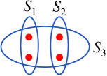
Figure 5: A toy set-cover instance with $K=4$ and $N=3$, where $\varphi(S_{1})=\frac{1}{2}$, $\varphi(S_{2})=1$, $\varphi(S_{3})=2$. In this case, the optimal set-cover is $\{S_{1},S_{2}\}$ and has a cost of $\frac{3}{2}$.

The above problem can be expressed as the following ILP:

$$\underset{\begin{subarray}{c}{x=(x^{(j)})_{1\leq j\leq N}}\end{subarray}}{\mathrm{minimize}}\;\;\sum_{j=1}^{N}\varphi(S_{j})\,x^{(j)}\$$ (36)

$$\quad\mathrm{s.t.}\;\;(\forall i\in\{1,\ldots,K\})\quad\sum_{\begin{subarray}{c}j\in\{1,\ldots,N\}\\ \upsilon^{(i)}\in S_{j}\end{subarray}}x^{(j)}\geq 1,\quad\;x\in\{0,1\}^{N},$$ (37)

where indicator variables $(x^{(j)})_{1\leq j\leq N}$ are used for determining if a set in $\mathcal{S}$ has been included in the set cover or not, and (37) ensures that each one of the elements of $\mathcal{V}$ is contained in at least one of the sets that were chosen for participating to the set cover.

An LP-relaxation for this problem is obtained by simply replacing the Boolean constraint with the constraint $x\in[0,+\infty[^{N}$. The dual of this LP relaxation is given by the following linear program:

$$\underset{\begin{subarray}{c}{y=(y^{(i)})_{1\leq i\leq K}\in[0,+\infty[^{K}}\end{subarray}}{\mathrm{maximize}}\;\;\sum_{i=1}^{K}y^{(i)}\$$ (38)

$$\quad\mathrm{s.t.}\;\;(\forall j\in\{1,\ldots,N\})\quad\sum_{\begin{subarray}{c}i\in\{1,\ldots,K\}\\ \upsilon^{(i)}\in S_{j}\end{subarray}}y^{(i)}\leq\varphi(S_{j}).$$ (39)

Let us denote by $F_{\max}$ the maximum frequency of an element in $\mathcal{V}$, where by the term frequency we mean the number of sets this element belongs to. In this case, we will use the primal-dual schema to derive an $F_{\max}$-approximation algorithm by choosing $\nu_{\mathrm{primal}}=1$, $\nu_{\mathrm{dual}}=F_{\max}$. This results into the following complementary slackness conditions, which we will need to satisfy:

Primal Complementary Slackness Conditions

$$(\forall j\in\{1,\ldots,N\})\text{ if }x^{(j)}>0\text{ then }\sum_{\begin{subarray}{c}i\in\{1,\ldots,K\}\\ \upsilon^{(i)}\in S_{j}\end{subarray}}y^{(i)}=\varphi(S_{j})$$ (40)

Relaxed Dual Complementary Slackness Conditions (with relaxation factor $F_{\max}$)

$$(\forall i\in\{1,\ldots,K\})\text{ if }y^{(i)}>0\text{ then }\sum_{\begin{subarray}{c}j\in\{1,\ldots,N\}\\ \upsilon^{(i)}\in S_{j}\end{subarray}}x^{(j)}\leq F_{\max}.$$ (41)

A set $S_{j}$ with $j\in\{1,\ldots,N\}$ for which $\sum_{\begin{subarray}{c}i\in\{1,\ldots,K\}\\ \upsilon^{(i)}\in S_{j}\end{subarray}}y^{(i)}=\varphi(S_{j})$ will be called packed. Based on this definition, and given that the primal variables $(x^{(j)})_{1\leq j\leq N}$ are always kept integral (i.e., either $0$ or $1$) during the primal-dual schema, Conditions (40) basically say that only packed sets can be included in the set cover (note that overpacked sets are already forbidden by feasibility constraints (39)). Similarly, Conditions (41) require that an element $\upsilon^{(i)}$ with $i\in\{1,\ldots,K\}$ associated with a nonzero dual variable $y^{(i)}$ should not be covered more than $F_{\max}$ times, which is, of course, trivially satisfied given that $F_{\max}$ represents the maximum frequency of any element in $\mathcal{V}$.

Algorithm 9 Primal-dual schema for set-cover.

$$\begin{array}[]{l}\text{Set}\;x_{0}\leftarrow 0,y_{0}\leftarrow 0\\ \text{Declare all elements in $\mathcal{V}$ as uncovered}\\ \text{While $\mathcal{V}$ contains uncovered elements}\\ \left\lfloor\begin{array}[]{l}\text{Select an uncovered element $\upsilon^{(i)}$ with $i\in\{1,\ldots,K\}$ and increase $y^{(i)}$ until some set becomes packed}\\ \text{For every packed set $S_{j}$ with $j\in\{1,\ldots,N\}$, set $x^{(j)}\leftarrow 1$}\\ \qquad\text{(include all the sets that are packed in the cover)}\\ \text{Declare all the elements belonging to at least one set $S_{j}$ with $x^{(j)}=1$ as covered.}\end{array}\right.\end{array}$$

Based on the above observations, the iterative method whose pseudocode is shown in Algorithm 9 emerges naturally as a simple variant of Algorithm 8. Upon its termination, both $x$ and $y$ will be feasible given that there will be no uncovered element and no set that violates (39). Furthermore, given that the final pair $(x,y)$ satisfies the relaxed complementary slackness conditions with $\nu_{\mathrm{primal}}=1$, $\nu_{\mathrm{dual}}=F_{\max}$, the set cover defined by $x$ will provide an $F_{\max}$-approximate solution.

IV-C Dual decomposition

We will next examine a different approach for discrete optimization, which is based on the principle of dual decomposition [14, 72, 1]. The core idea behind this principle essentially follows a divide and conquer strategy: that is, given a difficult or high-dimensional optimization problem, we decompose it into smaller easy-to-handle subproblems and then extract an overall solution by cleverly combining the solutions from these subproblems.

To explain this technique, we will consider the general problem of minimizing the energy of a discrete Markov Random Field (MRF), which is a ubiquitous problem in the fields of computer vision and image analysis (applied with great success on a wide variety of tasks from these domains such as stereo-matching, image segmentation, optical flow estimation, image restoration and inpainting, or object detection) [2]. This problem involves a graph $G$ with vertex set $\mathcal{V}$ and edge set $\mathcal{E}$ (i.e., $G=(\mathcal{V},\mathcal{E})$) plus a finite label set $\mathcal{L}$. The goal is to find a labeling $z=(z^{(p)})_{p\in\mathcal{V}}\in\mathcal{L}^{|\mathcal{V}|}$ for the graph vertices that has minimum cost, that is

$$\underset{\begin{subarray}{c}{z\in\mathcal{L}^{|\mathcal{V}|}}\end{subarray}}{\mathrm{minimize}}\;\;\sum_{p\in\mathcal{V}}\varphi_{p}(z^{(p)})+\sum_{e\in\mathcal{E}}\sansmath\varphi_{e}(\mathsf{z}^{(e)})$$ (42)

where, for every $p\in\mathcal{V}$ and $e\in\mathcal{E}$, $\varphi_{p}\colon\mathcal{L}\to\,\left]-\infty,+\infty\right[$ and $\sansmath\varphi_{e}\colon\mathcal{L}^{2}\to\,\left]-\infty,+\infty\right[$ represent the unary and pairwise costs (also known connectively as MRF potentials $\varphi=\left\{\{\varphi_{p}\}_{p\in\mathcal{V}},\{\sansmath\varphi_{e}\}_{e\in\mathcal{E}}\right\}$), and $\mathsf{z}^{(e)}$ denotes the pair of components of $z$ defined by the variables corresponding to vertices connected by $e$ (i.e., $\mathsf{z}^{(e)}=(z^{(p)},z^{(q)})$ for $e=(p,q)\in\mathcal{E}$).

The above problem is NP-hard, and much of the recent work on MRF optimization revolves around the following equivalent ILP formulation of (42) [73], which is the one that we will also use here:

$$\underset{\begin{subarray}{c}{x\in C_{G}}\end{subarray}}{\mathrm{minimize}}\;\;f(x;\varphi)=\sum_{p\in\mathcal{V},\,z^{(p)}\in\mathcal{L}}\varphi_{p}(z^{(p)})\,x_{p}(z^{(p)})+\sum_{e\in\mathcal{E},\,\mathsf{z}^{(e)}\in\mathcal{L}^{2}}\sansmath\varphi_{e}(\mathsf{z}^{(e)})\,\mathsf{x}_{e}(\mathsf{z}^{(e)}),$$ (43)

where the set $C_{G}$ is defined for any graph $G=(\mathcal{V},\mathcal{E})$ as

$$C_{G}=\left\{{x=\big{\{}\{x_{p}\}_{p\in\mathcal{V},z\in\mathcal{L}},\{\mathsf{x}_{e}\}_{e\in\mathcal{V},\mathsf{z}\in\mathcal{L}^{2}}\big{\}}}\left|\begin{array}[]{l}(\forall p\in\mathcal{V})\qquad\qquad\qquad\qquad\quad\;\sum_{z^{(p)}\in\mathcal{L}}x_{p}(z^{(p)})=1\\ (\forall e=(p,q)\in\mathcal{E})(\forall z^{(q)}\in\mathcal{L})\quad\sum_{\mathsf{z}^{(e)}\in\mathcal{L}\times\{z^{(q)}\}}\mathsf{x}_{e}(\mathsf{z}^{(e)})=x_{q}(z^{(q)})\\ (\forall e=(p,q)\in\mathcal{E})(\forall z^{(p)}\in\mathcal{L})\quad\sum_{\mathsf{z}^{(e)}\in\{z^{(p)}\}\times\mathcal{L}}\mathsf{x}_{e}(\mathsf{z}^{(e)})=x_{p}(z^{(p)})\\ {(\forall p\in\mathcal{V})\qquad\qquad\qquad\qquad\qquad x_{p}(\cdot)\colon\mathcal{L}\mapsto\{0,1\}}\\ {(\forall e\in\mathcal{E})\qquad\qquad\qquad\qquad\qquad\mathsf{x}_{e}(\cdot)\colon\mathcal{L}^{2}\to\{0,1\}}\end{array}\right.\right\}.$$ (44)

In the above formulation, for every $p\in\mathcal{V}$ and $e\in\mathcal{E}$, the unary binary function $x_{p}(\cdot)$ and the pairwise binary function $\mathsf{x}_{e}(\cdot)$ indicate the labels assigned to vertex $p$ and to the pair of vertices connected by edge $e=(p^{\prime},q^{\prime})$ respectively, i.e.,

$$(\forall z^{(p)}\in\mathcal{L})\qquad\qquad\qquad\qquad\;\;x_{p}(z^{(p)})=1\quad\Leftrightarrow\quad p\text{ is assigned label }z^{(p)}$$ (45)

$$(\forall\mathsf{z}^{(e)}=(z^{(p^{\prime})},z^{(q^{\prime})})\in\mathcal{L}^{2})\qquad\mathsf{x}_{e}(\mathsf{z}^{(e)})=1\quad\Leftrightarrow\quad p^{\prime},q^{\prime}\text{ are assigned labels }z^{(p^{\prime})},z^{(q^{\prime})}.$$ (46)

Minimizing with respect to the vector $x$ regrouping all these binary functions is equivalent to searching for an optimal binary vector of dimension $N=|\mathcal{V}||\mathcal{L}|+|\mathcal{E}||\mathcal{L}|^{2}$. The first constraints in (44) simply encode the fact that each vertex must be assigned exactly one label, whereas the rest of the constraints enforces consistency between unary functions $x_{p}(\cdot)$, $x_{q}(\cdot)$ and the pairwise function $\mathsf{x}_{e}(\cdot)$ for edge $e=(p,q)$, ensuring essentially that if $x_{p}(z^{(p)})=x_{q}(z^{(q)})=1$, then $\mathsf{x}_{e}(z^{(p)},z^{(q)})=1$.

As mentioned above, our goal will be to decompose the MRF problem (43) into easier subproblems (called slaves), which, in this case, involve optimizing MRFs defined on subgraphs of $G$. More specifically, let $\{G_{m}=(\mathcal{V}_{m},\mathcal{E}_{m})\}_{1\leq m\leq M}$ be a set of subgraphs that form a decomposition of $G=(\mathcal{V},\mathcal{E})$ (i.e., $\displaystyle\cup_{m=1}^{M}\mathcal{V}_{m}=\mathcal{V}$, $\displaystyle\cup_{m=1}^{M}\mathcal{E}_{m}=\mathcal{E}$). On each of these subgraphs, we define a local MRF with corresponding (unary and pairwise) potentials $\varphi^{m}=\left\{\{\varphi^{m}_{p}\}_{p\in\mathcal{V}_{m}},\{\sansmath\varphi^{m}_{e}\}_{e\in\mathcal{E}_{m}}\right\}$, whose cost function $f^{m}(x;\varphi^{m})$ is thus given by

$$f^{m}(x;\varphi^{m})=\sum_{p\in\mathcal{V}_{m},\,z^{(p)}\in\mathcal{L}}\varphi^{m}_{p}(z^{(p)})\,x_{p}(z^{(p)})+\sum_{e\in\mathcal{E}_{m},\,\mathsf{z}^{(e)}\in\mathcal{L}^{2}}\sansmath\varphi^{m}_{e}(\mathsf{z}^{(e)})\,\mathsf{x}_{e}(\mathsf{z}^{(e)}).$$ (47)

Moreover, the sum (over $m$) of the potential functions $\varphi^{m}$ is ensured to give back the potentials $\varphi$ of the original MRF on $G$, i.e.,

$$(\forall p\in\mathcal{V})(\forall e\in\mathcal{E})\quad\sum_{\begin{subarray}{c}m\in\{1,\ldots,M\}:p\in\mathcal{V}_{m}\end{subarray}}\mspace{-10.0mu}\varphi^{m}_{p}=\varphi_{p},\quad\sum_{\begin{subarray}{c}m\in\{1,\ldots,M\}:e\in\mathcal{E}_{m}\end{subarray}}\mspace{-10.0mu}\sansmath\varphi^{m}_{e}=\sansmath\varphi_{e}.$$ (48)

This guarantees that $f=\sum_{m=1}^{M}f^{m}$, thus allowing us to re-express problem (43) as follows

$$\underset{\begin{subarray}{c}{x\in C_{G}}\end{subarray}}{\mathrm{minimize}}\;\;\sum_{m=1}^{M}f^{m}(x;\varphi^{m}).$$ (49)

An assumption that often holds in practice is that minimizing separately each of the $f^{m}$ (over $x$) is easy, but minimizing their sum is hard. Therefore, to leverage this fact, we introduce, for every $m\in\{1,\ldots,M\}$, an auxiliary copy $x^{m}\in C_{G_{m}}$ for the variables of the local MRF defined on $G_{m}$, which are thus constrained to coincide with the corresponding variables in vector $x$, i.e., it holds $x^{m}=x_{|G_{m}}$, where $x_{|G_{m}}$ is used to denote the subvector of $x$ containing only those variables associated with vertices and edges of subgraph $G_{m}$. In this way, Problem (49) can be transformed into

$$\underset{\begin{subarray}{c}{x\in C_{G},\{x^{m}\in C_{G_{m}}\}_{1\leq m\leq M}}\end{subarray}}{\mathrm{minimize}}\;\; \sum_{m=1}^{M}f^{m}(x^{m};\varphi^{m})$$

$$\mathrm{s.t.} \ \ \big{(}\forall m\in\{1,\ldots,M\}\big{)}\qquad x^{m}=x_{|G_{m}}.$$ (50)

By considering the dual of (IV-C), using a technique similar to the one described in framebox on page II-D, and noticing that

$$x\in C_{G}\quad\Leftrightarrow\quad(\forall m\in\{1,\ldots,M\})\quad x^{m}\in C_{G_{m}},$$ (51)

we finally end up with the following problem:

$$\underset{\begin{subarray}{c}{(v^{m})_{1\leq m\leq M}\in\Lambda}\end{subarray}}{\mathrm{maximize}}\;\;\sum_{m=1}^{M}h^{m}(v^{m}),$$ (52)

where, for every $m\in\{1,\ldots,M\}$, the dual variable $v^{m}$ consists of $\left\{\{v^{m}_{p}\}_{p\in\mathcal{V}_{m}},\{\mathsf{v}^{m}_{e}\}_{e\in\mathcal{E}_{m}}\right\}$ similarly to $\varphi^{m}$, and function $h^{m}$ is related to the following optimization of a slave MRF on $G_{m}$:

$$h^{m}(v^{m})=\min_{x^{m}\in C_{G_{m}}}f^{m}(x^{m};\varphi^{m}+v^{m}).$$ (53)

The feasible set $\Lambda$ is given by

$$\Lambda=\left\{{v=\left\{\{v^{m}_{p}\}_{p\in\mathcal{V}_{m}},\{\mathsf{v}^{m}_{e}\}_{e\in\mathcal{E}_{m}}\right\}_{1\leq m\leq M}}\left|\begin{array}[]{l}(\forall p\in\mathcal{V})(\forall z^{(p)}\in\mathcal{L})\quad\qquad\;\sum\limits_{\begin{subarray}{c}m\in\{1,\ldots,M\}:p\in\mathcal{V}_{m}\end{subarray}}v^{m}_{p}(z^{(p)})=0,\\ (\forall e\in\mathcal{E})(\forall\mathsf{z}^{(e)}\in\mathcal{L}^{2})\quad\qquad\sum\limits_{\begin{subarray}{c}m\in\{1,\ldots,M\}:e\in\mathcal{E}_{m}\end{subarray}}\mathsf{v}^{m}_{e}(\mathsf{z}^{(e)})=0\\ {(\forall m\in\{1,\ldots,M\})(\forall p\in\mathcal{V})\;\;v^{m}_{p}(\cdot)\colon\mathcal{L}\mapsto\mathbb{R}}\\ {(\forall m\in\{1,\ldots,M\})(\forall e\in\mathcal{E})\;\;\mathsf{v}^{m}_{e}(\cdot)\colon\mathcal{L}^{2}\mapsto\mathbb{R}}\end{array}\right.\right\}.$$ (54)

The above dual problem provides a relaxation to the original problem (43)-(44). Furthermore, note that this relaxation leads to a convex optimization problem, although the original one is not. As such, it can always be solved in an optimal manner. A possible way of doing this consists of using a projected subgradient method. Exploiting the form of the projection onto the vector space $\Lambda$ yields Algorithm 10 where $(\gamma_{n})_{n\in\mathbb{N}}$ is a summable sequence of positive step-sizes and $\left\{\{\widehat{x}^{m}_{p,n}\}_{p\in\mathcal{V}_{m}},\{\widehat{\mathsf{x}}^{m}_{e,n}\}_{e\in\mathcal{E}_{m}}\right\}$ corresponds to a subgradient of function $h^{m}$ with $m\in\{1,\ldots,M\}$ computed at iteration $n$ [14]. Note that this algorithm requires only solutions to local subproblems to be computed, which is, of course, a task much easier that furthermore can be executed in a parallel manner. The solution to the master MRF is filled in from local solutions $\left\{\{\widehat{x}^{m}_{p,n}\}_{p\in\mathcal{V}_{m}},\{\widehat{\mathsf{x}}^{m}_{e,n}\}_{e\in\mathcal{E}_{m}}\right\}_{1\leq m\leq M}$ after convergence of the algorithm.

Algorithm 10 Dual decomposition for MRF optimization.

$$\begin{array}[]{l}\text{Choose a decomposition $\{G_{m}=(\mathcal{V}_{m},\mathcal{E}_{m})\}_{1\leq m\leq M}$ of $G$}\\ \text{Initialize potentials of slave MRFs:}\\ (\forall m\in\{1,\ldots,M\})(\forall p\in\mathcal{V}_{m})\;\varphi^{m}_{p,0}=\frac{\varphi_{p}}{|\{m^{\prime}\mid p\in\mathcal{V}_{m^{\prime}}\}|},(\forall e\in\mathcal{E}_{m})\;\sansmath\varphi^{m}_{e,0}=\frac{\sansmath\varphi_{e}}{|\{m^{\prime}\mid e\in\mathcal{E}_{m^{\prime}}\}|}\\ \text{for}\;n=0,\ldots\\ \left\lfloor\begin{array}[]{l}\text{Compute minimizers of slave MRF problems:}\;(\forall m\in\{1,\ldots,M\})\;\left\{\{\widehat{x}^{m}_{p,n}\}_{p\in\mathcal{V}_{m}},\{\widehat{\mathsf{x}}^{m}_{e,n}\}_{e\in\mathcal{E}_{m}}\right\}\in\underset{\begin{subarray}{c}{x^{m}\in C_{G_{m}}}\end{subarray}}{\mathrm{Argmin}}\;\;f^{m}(x^{m};\varphi^{m}_{n})\\ \text{Update potentials of slave MRFs:}\\ (\forall m\in\{1,\ldots,M\})(\forall p\in\mathcal{V}_{m})\;\varphi^{m}_{p,n+1}=\varphi^{m}_{p,n+1}+\gamma_{n}\left(\widehat{x}^{m}_{p,n}-\frac{\sum_{m:\,p\in\mathcal{V}_{m}}{\widehat{x}^{m}_{p,n}}}{|\{m^{\prime}\mid p\in\mathcal{V}_{m^{\prime}}\}|}\right)\\ (\forall m\in\{1,\ldots,M\})(\forall e\in\mathcal{E}_{m})\;\sansmath\varphi^{m}_{e,n+1}=\sansmath\varphi^{m}_{e,n}+\gamma_{n}\left(\widehat{\mathsf{x}}^{m}_{e,n}-\frac{\sum_{m:\,e\in\mathcal{E}_{m}}{\widehat{\mathsf{x}}^{m}_{e,n}}}{|\{m^{\prime}\mid p\in\mathcal{V}_{m^{\prime}}\}|}\right).\\ \end{array}\right.\end{array}$$

For a better intuition for the updates of variables $\left\{\{\varphi^{m}_{p,n}\}_{p\in\mathcal{V}_{m}},\{\sansmath\varphi^{m}_{e,n}\}_{e\in\mathcal{E}_{m}}\right\}_{1\leq m\leq M,n\in\mathbb{N}}$ in Algorithm 10, we should note that their aim is essentially to bring a consensus among the solutions of the local subproblems. In other words, they try to adjust the potentials of the slave MRFs so that in the end the corresponding local solutions are consistent with each other, i.e., all variables corresponding to a common vertex or edge are assigned the same value by the different subproblems. If this condition is satisfied (i.e., there is a full consensus) then the overall solution that results from combining the consistent local solutions is guaranteed to be optimal. In general, though, this might not always be true given that the above procedure is solving only a relaxation of the original NP-hard problem.

MASTER-SLAVE COMMUNICATION During dual decomposition a communication between a master process and the slaves (local subproblems) can be thought of as taking place, which can also be interpreted as a resource allocation/pricing stage. Resource allocation: At each iteration, the master assigns new MRF potentials (i.e., resources) $(\varphi^{m})_{1\leq m\leq M}$ to the slaves based on the current local solutions $(\widehat{x}^{m})_{1\leq m\leq M}$. Pricing: The slaves respond by adjusting their local solutions $(\widehat{x}^{m})_{1\leq m\leq M}$ (i.e., the prices) so as to maximize their welfares based on the newly assigned resources $(\widehat{x}^{m})_{1\leq m\leq M}$.

DECOMPOSITIONS AND RELAXATIONS Different decompositions can lead to different relaxations and/or can affect the speed of convergence. We show below, for instance, 3 possible decompositions for an MRF assumed to be defined on a $5\times 5$ image grid. Decompositions $\{G^{1}_{m}\},\{G^{2}_{m}\},\{G^{3}_{m}\}$ consist respectively of one suproblem per row and column, one subproblem per edge, and one subproblem per $2\times 2$ subgrid of the original $5\times 5$ grid. Both $\{G^{1}_{m}\}$ and $\{G^{2}_{m}\}$ (due to using solely subgraphs that are trees) lead to the same LP relaxation of (43), whereas $\{G^{3}_{m}\}$ leads to a relaxation that is tighter (due to containing loopy subgraphs). On the other hand, decomposition $\{G^{1}_{m}\}$ leads to faster convergence compared with $\{G^{2}_{m}\}$ due to using larger subgraphs that allow a faster propagation of information during message-passing.

Interestingly, if we choose to use a decomposition consisting only of subgraphs that are trees, then the resulting relaxation can be shown to actually coincide with the standard LP-relaxation of linear integer program (43) (generated by replacing the integrality constraints with non-negativity constraints on the variables). This also means that when this LP-relaxation is tight, an optimal MRF solution is computed. This, for instance, leads to the result that dual decomposition approaches can estimate a globally optimal solution for binary submodular MRFs (although it should be noted that much faster graph-cut based techniques exist for submodular problems of this type - see framebox on page IV-C). Furthermore, when using subgraphs that are trees, a minimizer to each slave problem can be computed efficiently by applying the Belief Propagation algorithm [74], which is a message-passing method. Therefore, in this case, Algorithm 10 essentially reduces to a continuous exchange of messages between the nodes of graph $G$. Such an algorithm relates to or generalizes various other message-passing approaches [15, 75, 76, 77, 78, 79]. In general, besides tree-structured subgraphs, other types of decompositions or subproblems can be used as well (such as binary planar problems, or problems on loopy subgraphs with small tree-width, for which MRF optimization can still be solved efficiently), which can lead to even tighter relaxations (see framebox on page IV-C) [80, 81, 82, 83, 84, 85].

GRAPH-CUTS AND MRF OPTIMIZATION For certain MRFs, optimizing their cost is known to be equivalent to solving a polynomial mincut problem [86, 87]. These are exactly all the binary MRFs ($|\mathcal{L}|=2$) with submodular pairwise potentials such that, for every $e\in\mathcal{E}$, $$\sansmath\varphi_{e}(0,0)+\sansmath\varphi_{e}(1,1)\leq\sansmath\varphi_{e}(0,1)+\sansmath\varphi_{e}(1,0).$$ (55) Due to (55), the cost $f(x)$ of a binary labeling $x=(x^{(p)})_{1\leq p\leq|\mathcal{V}|}\in\{0,1\}^{|\mathcal{V}|}$ for such MRFs can always be written (up to an additive constant) as $$f(x)=\sum_{p\in\mathcal{V}_{P}}a_{p}x^{(p)}+\sum_{p\in\mathcal{V}_{N}}a^{(p)}(1-x^{(p)})+\sum_{(p,q)\in\mathcal{E}}a_{p,q}x^{(p)}(1-x^{(q)}),$$ (56) where all coefficients $(a_{p})_{p\in\mathcal{V}}$ and $(a_{p,q})_{(p,q)\in\mathcal{E}}$ are nonnegative ($\mathcal{V}_{P}\subset\mathcal{V}$, $\mathcal{V}_{N}\subset\mathcal{V}$). In this case, we can associate to $f$ a capacitated network that has vertex set $\mathcal{V}_{f}=\mathcal{V}\cup\{s,t\}$. A source vertex $s$ and a sink one $t$ have thus been added. The new edge set $\mathcal{E}_{f}$ is deduced from the one used to express $f$: $$\mathcal{E}_{f}=\{(p,t)\mid p\in\mathcal{V}_{P}\}\cup\{(s,p)\mid p\in\mathcal{V}_{N}\}\cup\mathcal{E},$$ and its edge capacities are defined as $(\forall p\in\mathcal{V}_{P}\cup\mathcal{V}_{N})$ $c_{p,t}=c_{s,p}=a_{p}$, and $(\forall(p,q)\in\mathcal{E})$ $c_{p,q}=a_{p,q}$. A one-to-one correspondence between $s$-$t$ cuts and MRF labelings then exists: $$x\in\{0,1\}^{|\mathcal{V}|}\leftrightarrow\mathrm{cut}(x)=\{s\}\cup\{p\mid x^{(p)}=1\}$$ for which it is easy to see that $$f(x)=\sum_{u\in\mathrm{cut}(x),\upsilon\notin\mathrm{cut}(x)}c_{u,\upsilon}=\text{cost of }\mathrm{cut}(x)\enspace.$$ Computing a mincut, in this case, solves the LP relaxation of (43), which is tight, whereas computing a max-flow solves the dual LP.

Furthermore, besides the projected subgradient method, one can alternatively apply an ADMM scheme for solving relaxation (52) (see Section III-B). The main difference, in this case, is that the optimization of a slave MRF problem is performed by solving a (usually simple) local quadratic problem, which can again be solved efficiently for an appropriate choice of the decomposition (see Section III-F). This method again penalizes disagreements among slaves, but it does so even more aggressively than the subgradient method since there is no longer a requirement for step-sizes $(\gamma_{n})_{n\in\mathbb{N}}$ converging to zero. Furthermore, alternative smoothed accelerated schemes exist and can be applied as well [88, 89, 90].

V Applications

Although the presented primal-dual algorithms can be applied virtually to any area where optimization problems have to be solved, we now mention a few common applications of these techniques.

V-A Inverse problems

For a long time, convex optimization approaches have been successfully used for solving inverse problems such as signal restoration, signal reconstruction, or interpolation of missing data. Most of the time, these problems are ill-posed and, in order to recover the signal of interest in a satisfactory manner, some prior information needs to be introduced. To do this, an objective function can be minimized which includes a data fidelity term modelling knowledge about the noise statistics and possibly involves a linear observation matrix (e.g. a convolutive blur), and a regularization (or penalization) term which corresponds to the additional prior information. This formulation can also often be justified statistically as the determination of a Maximum A Posteriori (MAP) estimate. In early developed methods, in particular in Tikhonov regularization, a quadratic penalty function is employed. Alternatively, hard constraints can be imposed on the solution (for example, bounds on the signal values), leading to signal feasibility problems. Nowadays, a hybrid regularization [91] may be prefered so as to combine various kinds of regularity measures, possibly computed for different representations of the signal (Fourier, wavelets,…), some of them like total variation [25] and its nonlocal extensions [92] being taylored for preserving discontinuities such as image edges. In this context, constraint sets can be translated into penalization terms being equal to the indicator functions of these sets (see (2)). Altogether, these lead to global cost functions which can be quite involved, often with many variables, for which the splitting techniques described in Section III-F are very useful. An extensive literature exists on the use of ADMM methods for solving inverse problems (e.g., see [29, 30, 31, 32, 33]). With the advent of more recent primal-dual algorithms, many works have been mainly focused on image recovery applications [46, 47, 48, 49, 51, 62, 54, 58, 55, 64, 93, 94, 95, 96, 97]. Two illustrations are now provided.

In [98], a generalization of the total variation is defined for an arbitrary graph in order to address a variety of inverse problems. For denoising applications, the optimization problem to be solved is of the form (19) where

$$f=0,\qquad g=\sigma_{C},\qquad h\colon x\mapsto\frac{1}{2}\|x-y\|^{2},$$ (57)

$x$ is a vector of variables associated with each vertex of a weighted graph, and $y\in\mathbb{R}^{N}$ is a vector of data observed at each vertex. The matrix $L\in\mathbb{R}^{K\times N}$ is equal to $\operatorname{Diag}(\sqrt{\omega}_{1},\ldots,\sqrt{\omega}_{K})\,A$ where $(\omega_{1},\ldots\omega_{K})\in\left[0,+\infty\right[^{K}$ is the vector of edge weights and $A\in\mathbb{R}^{K\times N}$ is the graph incidence matrix playing a role similar to a gradient operator on the graph. The set $C$ is defined as an intersection of closed semi-balls in such a way that its support function $\sigma_{C}$ (see (9)) allows us to define a class of functions extending the total variation semi-norm (see [98] for more details). Good image denoising results can be obtained by building the graph in a nonlocal manner following the strategy in [92]. Results obtained for Barbara image are displayed in Fig. 6. Interestingly, the ability of methods such as those presented in Section III-D to circumvent matrix inversions leads to a significant decrease of the convergence time for irregular graphs in comparison with algorithms based on the Douglas-Rachford iteration or ADMM (see Fig. 7).

(a) Original image

(b) Noisy SNR = $14.47$ dB

(c) Nonlocal TV SNR = $20.78$ dB

Figure 6: Nonlocal denoising (additive white zero-mean Gaussian noise with variance $\sigma^{2}=20$).

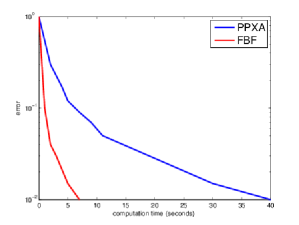
Figure 7: Comparison of the convergence speed of a Douglas-Rachford based algorithm (PPXA [65]) (blue) and an FBF-based primal-dual algorithm (red) for image denoising using a non-regular graph, Matlab implementation on an Intel Xeon 2.5GHz 8-core system.

Another application example of primal-dual proximal algorithms is Parallel Magnetic Resonance Imaging (PMRI) reconstruction. A set of measurement vectors $(z_{j})_{1\leq j\leq J}$ is acquired from $J$ coils. These observations are related to the original full FOV (Field Of View) image $\overline{x}\in\mathbb{C}^{N}$ corresponding to a spin density. An estimate of $\overline{x}$ is obtained by solving the following problem:

$$\underset{\begin{subarray}{c}{x\in\mathbb{C}^{N}}\end{subarray}}{\mathrm{minimize}}\;\;f(x)+g(Lx)+\underbrace{\sum_{j=1}^{J}\|\Sigma FS_{j}x-z_{j}\|^{2}_{\Lambda_{j}^{-1}}}_{\mbox{$h(x)$}}$$ (58)

where $(\forall j\in\{1,\ldots,J\})$ $\|\cdot\|^{2}_{\Lambda_{j}^{-1}}=(\cdot)^{\rm H}\Lambda_{j}^{-1}(\cdot)$, $\Lambda_{j}$ is the noise covariance matrix for the $j$-the channel, $S_{j}\in\mathbb{C}^{N\times N}$ is a diagonal matrix modelling the sensitivity of the coil, $F\in\mathbb{C}^{N\times N}$ is a 2D discrete Fourier transform, $\Sigma\in\{0,1\}^{\lfloor\frac{N}{R}\rfloor\times N}$ is a subsampling matrix, $g\in\Gamma_{0}(\mathbb{C}^{K})$ is a sparsity measure (e.g. a weighted $\ell_{1}$-norm), $L\in\mathbb{C}^{K\times N}$ is a (possibly redundant) frame analysis operator, and $f$ is the indicator function of a vector subspace of $\mathbb{C}^{N}$ serving to set to zero the image areas corresponding to the background. Combining suitable subsampling strategies in the k-space with the use of an array of coils allows us to reduce the acquisition time while maintaining a good image quality. The subsampling factor $R>1$ thus corresponds to an acceleration factor. For a more detailed account on the considered approach, the reader is refered to [99, 100] and the references therein. Reconstruction results are shown in Fig. 8. Fig. 9 also allows us to evaluate the convergence time for various algorithms. It can be observed that smaller differences between the implemented primal-dual strategies are apparent in this example. Due to the form of the subsampling matrix, the matrix inversion involved at each iteration of ADMM however requires to make use of a few subiterations of a linear conjugate gradient method.

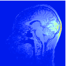
Figure 8: (a) Effects of the sensitivity matrices in the spatial domain in the absence of subsampling: the moduli of the images corresponding to $(S_{j}\overline{x})_{2\leq j\leq 3}$ are displayed for 2 channels out of 32. (b) Reconstruction quality: moduli of the original slice $\overline{x}$ and the reconstructed one with SNR = $20.03$ dB (from left to right) using polynomial sampling of order 1 with $R=5$, a wavelet frame, and an $\ell_{1}$ regularization.

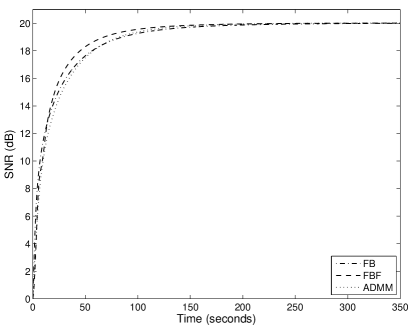
Figure 9: Signal-to-Noise Ratio as a function of computation time using ADMM, and FB or FBF-based primal-dual methods for a given slice, Matlab implementation on an Intel i7-3520M CPU@2.9 GHz system.

Note that convex primal-dual proximal optimization algorithms have been applied to other fields than image recovery, in particular to machine learning [5, 101], system identification [102], audio processing [103], optimal transport [104], empirical mode decomposition [105], seimics [106], database management [107], and data streaming over networks [108].

V-B Computer vision and image analysis

The great majority of problems in computer vision involve image observation data that are of very high dimensionality, inherently ambiguous, noisy, incomplete, and often only provide a partial view of the desired space. Hence, any successful model that aims to explain such data usually requires a reasonable regularization, a robust data measure, and a compact structure between the variables of interest to efficiently characterize their relationships. Probabilistic graphical models, and in particular discrete Markov Random Fields, have led to a suitable methodology for solving such visual perception problems [12, 16]. This type of models offer great representational power, and are able to take into account dependencies in the data, encode prior knowledge, and model (soft or hard) contextual constraints in a very efficient and modular manner. Furthermore, they offer the important ability to make use of very powerful data likelihood terms consisting of arbitrary nonconvex and non-continuous functions that are often crucial for accurately representing the problem at hand. As a result, MAP-inference for these models leads to discrete optimization problems that are (in most cases) highly nonconvex (NP-hard) and also of very large scale [109, 110]. These discrete problems take the form (42), where typically the unary terms $\varphi_{p}(\cdot)$ encode the data likelihood and the higher-order terms $\sansmath\varphi_{e}(\cdot)$ encode problem specific priors.

Primal-dual approaches can offer important computational advantages when dealing with such problems. One such characteristic example is the FastPD algorithm [13], which currently provides one of the most efficient methods for solving generic MRF optimization problems of this type, also guaranteeing at the same time the convergence to solutions that are approximately optimal. The theoretical derivation of this method relies on the use of the primal-dual schema described in Section IV, which results, in this case, into a very fast graph-cut based inference scheme that generalizes previous state-of-the-art approaches such as the $\alpha$-expansion algorithm [111] (see Fig. 10). More generally, due to the very wide applicability of MRF models to computer vision or image analysis problems, primal-dual approaches can and have been applied to a broad class of both low-level and high-level problems from these domains, including image segmentation [112, 113, 114, 115], stereo matching and 3D multi-view reconstruction [116, 117], graph-matching [118], 3D surface tracking [119], optical flow estimation [120], scene understanding [121], image deblurring [122], panoramic image stitching [123], category-level segmentation [124], and motion tracking [125]. In the following we mention very briefly just a few examples.

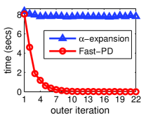
(a) ‘Penguin’ image denoising (from left to right: noisy input image, FastPD output, time comparison plot)

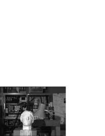
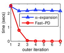
(b) ‘Tsukuba’ stereo matching (from left to right: left image, FastPD output, time comparison plot)

Fig. 10: FastPD [126] results for an image denoising (top) and stereo-matching (bottom) problem. The plot in each row compares the corresponding running time per iteration of the above primal-dual algorithm with the $\alpha$-expansion algorithm, which is a primal-based method (experiments conducted on a 1.6 GHz CPU).

A primal-dual based optimization framework has been recently proposed in [127, 128] for the problem of deformable registration/fusion, which forms one of the most central and challenging tasks in medical image analysis. This problem consists of recovering a nonlinear dense deformation field that aligns two signals that have in general an unknown relationship both in the spatial and intensity domain. In this framework, towards dimensionality reduction on the variables, the dense registration field is first expressed using a set of control points (registration grid) and an interpolation strategy. Then, the registration cost is expressed using a discrete sum over image costs projected on the control points, and a smoothness term that penalizes local deviations on the deformation field according to a neighborhood system on the grid. One advantage of the resulting optimization framework is that it is able to encode even very complex similarity measures (such as normalized mutual information and Kullback-Leibler divergence) and therefore can be used even when seeking transformations between different modalities (inter-deformable registration). Furthermore, it admits a broad range of regularization terms, and can also be applied to both 2D-2D and 3D-3D registration, as an arbitrary underlying graph structure can be readily employed (see Fig. 11 for a result on 3D inter-subject brain registration).

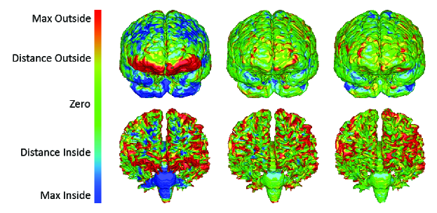
Fig. 11: Color encoded visualization of the surface distance between warped and expert segmentation after affine (left), FFD-based [129] (middle), and primal-dual based registration (right) for the Brain 1 data set. The color range is scaled to a maximum and minimum distance of 3 mm. The average surface distance (ASD) after registration for the gray matter is 1.66, 1.14, and 1.00 mm for affine, FFD-based, and primal-dual method, respectively. For the white matter the resulting ASD is 1.92, 1.31, and 1.06 mm. Note also that the FFD-based method is more than 30 times slower than the primal-dual approach.

Another application of primal-dual methods is in stereo reconstruction [130], where given as input a pair of left and right images $I_{L}$, $I_{R}$ we seek to estimate a function $u:\Omega\rightarrow\Gamma$ representing the depth $u(s)$ at a point $s$ in the domain $\Omega\subset\mathbb{R}^{2}$ of the left image (here $\Gamma=[\upsilon_{\rm min},\upsilon_{\rm max}]$ denotes the allowed depth range). To accomplish this, the following variational problem is proposed in [130]:

$$\underset{\begin{subarray}{c}{u}\end{subarray}}{\mathrm{minimize}}\;\;\int_{\Omega}f(u(s),s)ds+\int_{\Omega}|\nabla u(s)|ds,$$ (59)

where $f(u(s),s)$ is a data term favoring different depth values by measuring the absolute intensity differences of respective patches projected in the two input images, and the second term is a TV regularizer that promotes spatially smooth depth fields. The above problem is nonconvex (due to the use of the data term $f$), but it turns out that there exists an equivalent convex formulation obtained by lifting the original problem to a higher-dimensional space, in which $u$ is represented in terms of its level sets

$$\underset{\begin{subarray}{c}{\phi\in D}\end{subarray}}{\mathrm{minimize}}\;\;\int_{\Sigma}(|\nabla\phi(s,\upsilon)|+f(s,\upsilon)|\partial_{\upsilon}\phi(s,\upsilon)|)dsd\upsilon.$$ (60)

In the above formulation, $\Sigma=\Omega\times\Gamma$, $\phi\colon\Sigma\rightarrow\{0,1\}$ is a binary function such that $\phi(s,\upsilon)$ equals $1$ if $u(s)>\upsilon$ and $0$ otherwise, and the feasible set is defined as $D=\left\{\phi\colon\Sigma\rightarrow\{0,1\}\mid(\forall s\in\Omega)\,\phi(s,\upsilon_{\rm min})=1,\phi(s,\upsilon_{\rm max})=0\right\}$. A convex relaxation of the latter problem is obtained by using $D^{\prime}=\big{\{}\phi\colon\Sigma\rightarrow[0,1]\mid(\forall s\in\Omega)$$\phi(s,\upsilon_{\rm min})=1,\phi(s,\upsilon_{\rm max})=0\big{\}}$ instead of $D$. A discretized form of the resulting optimization problem can be solved with the algorithms described in Section III-C. Fig. 12 shows a sample result of this approach.

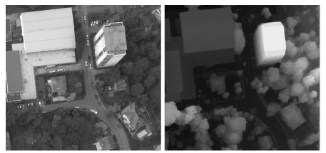
Fig. 12: Estimated depth map (right) for a large aerial stereo data set of Graz using the primal-dual approach in [130]. One of the images of the corresponding stereoscopic pair (of size $1500\times 1400$) is shown on the left.

Recently, primal-dual approaches have also been developed for discrete optimization problems that involve higher-order terms [131, 132, 133]. They have been applied successfully to various tasks, like, for instance, in stereo matching [131]. In this case, apart from a data term that measures similarity between corresponding pixels in two images, a discontinuity-preserving smoothness prior of the form $\sansmath\varphi(s_{1},s_{2},s_{3})=\min(|s_{1}-2s_{2}+s_{3}|,\kappa)$ with $\kappa\in\,\left]0,+\infty\right[$ has been employed as a regularizer that penalizes depth surfaces of high curvature. Indicative stereo matching results from an algorithm based on the dual decomposition principle described in Section IV-C are shown in Fig. 13.

It should be also mentioned that an advantage of all primal-dual algorithms (which is especially important for NP-hard problems) is that they also provide (for free) per-instance approximation bounds, specifying how far the cost of an estimated solution can be from the unknown optimal cost. This directly follows from the fact that these methods are computing both primal and dual solutions, which (in the case of a minimization task) provide respectively upper and lower limits to the true optimum. These approximation bounds are continuously updated throughout an algorithm execution, and thus can be directly used for assessing the performance of a primal-dual method with respect to any particular problem instance (and without essentially any extra computational cost). Moreover, often in practice, these sequences converge to a common value, which means that the corresponding estimated solutions are almost optimal (see, e.g., the plots in Fig. 13).

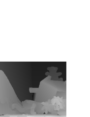
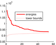
(a) ‘Teddy’

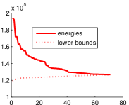
(b) ‘Cones’

Fig. 13: Stereo matching results for ‘Teddy’ (a) and ’Cones’ (b) when using a higher-order discontinuity preserving smoothness prior. We show plots for the corresponding sequences of upper and lower bounds generated during the primal-dual method. Notice that these sequences converge to the same limit, meaning that the estimated solution converges to the optimal value.

VI Conclusion

In this paper, we have reviewed a number of primal-dual optimization methods which can be employed for solving signal and image processing problems. The links existing between convex approaches and discrete ones were little explored in the literature and one of the contributions of this paper is to put them in a unifying perspective. Although the presented algorithms have been proved to be quite effective in numerous problems, there remains much room for extending their scope to other application fields, and also for improving them so as to accelerate their convergence. In particular, the parameter choices in these methods may have a strong influence on the convergence speed and it would be thus interesting to design automatic procedures for setting these parameters. Various techniques can also be devised for designing faster variants of these methods (preconditioning, activation of blocks of variables, combination with stochastic strategies, distributed implementations…). Another issue to pay attention to is the robustness to numerical errors although it can be mentioned that most of the existing proximal algorithms are tolerant to summable errors. Concerning discrete optimization methods, we have shown that the key to success lies in tight relaxations of combinatorial NP hard problems. Extending these methods to more challenging problems, e.g. those involving higher-order Markov fields or extremely large label sets, appears to be of main interest in this area. More generally, developing primal-dual strategies that further bridge the gap between continuous and discrete approaches, as well as for solving other kinds of nonconvex optimization problems such as those encountered in phase reconstruction or blind deconvolution opens the way to appealing investigations. So, the ground is yours now to play with duality!

References

- [1] D. P. Bertsekas, Nonlinear Programming, Athena Scientific, Nashua, NH, 2004, second edition.
- [2] A. Blake, P. Kohli, and C. Rother, Markov Random Fields for Vision and Image Processing, MIT Press, 2011.
- [3] S. Sra, S. Nowozin, and S. J. Wright, Optimization for Machine Learning, MIT Press, Cambridge, MA, 2012.
- [4] S. Theodoridis, Machine Learning: A Signal and Information Processing Perspective, Academic Press, 2014, to appear.
- [5] F. Bach, R. Jenatton, J. Mairal, and G. Obozinski, “Optimization with sparsity-inducing penalties,” Found. Trends in Machine Learn., vol. 4, no. 1, pp. 1–106, 2012.
- [6] R. T. Rockafellar, Convex Analysis, Princeton University Press, Princeton, NJ, 1970.
- [7] S. Boyd and L. Vandenberghe, Convex Optimization, Cambridge University Press, Cambridge, UK, 2004.
- [8] H. H. Bauschke and P. L. Combettes, Convex Analysis and Monotone Operator Theory in Hilbert Spaces, Springer, New York, 2011.
- [9] J. J. Moreau, “Proximité et dualité dans un espace hilbertien,” Bull. Soc. Math. France, vol. 93, pp. 273–299, 1965.
- [10] P. L. Combettes and J.-C. Pesquet, “Proximal splitting methods in signal processing,” in Fixed-Point Algorithms for Inverse Problems in Science and Engineering, H. H. Bauschke, R. S. Burachik, P. L. Combettes, V. Elser, D. R. Luke, and H. Wolkowicz, Eds., pp. 185–212. Springer-Verlag, New York, 2011.
- [11] P. L. Combettes and J.-C. Pesquet, “Primal-dual splitting algorithm for solving inclusions with mixtures of composite, Lipschitzian, and parallel-sum type monotone operators,” Set-Valued Var. Anal., vol. 20, no. 2, pp. 307–330, June 2012.
- [12] S. Z. Li, Markov Random Field Modeling in Image Analysis, Springer-Verlag, London, 3rd edition, 2009.
- [13] N. Komodakis, G. Tziritas, and N. Paragios, “Performance vs computational efficiency for optimizing single and dynamic MRFs: Setting the state of the art with primal-dual strategies,” Computer Vision and Image Understanding, vol. 112, pp. 14–29, 2008.
- [14] N. Komodakis, N. Paragios, and G. Tziritas, “MRF energy minimization and beyond via dual decomposition,” IEEE Trans. Pattern Anal. Mach. Int., vol. 33, no. 3, pp. 531–552, Jan. 2011.
- [15] M. Wainwright, T. Jaakkola, and A. Willsky, “MAP estimation via agreement on trees: message-passing and linear programming,” IEEE Trans. Inform. Theory, vol. 51, no. 11, pp. 3697–3717, Nov. 2005.
- [16] C. Wang, N. Komodakis, and N. Paragios, “Markov random field modeling, inference & learning in computer vision & image understanding: A survey,” Computer Vision and Image Understanding, vol. 117, no. 11, pp. 1610–1627, Nov. 2013.
- [17] V. V. Vazirani, Approximation Algorithms, Springer-Verlag, New York, NY, USA, 2001.
- [18] D. S. Hochbaum, Ed., Approximation Algorithms for NP-hard Problems, PWS Publishing Co., Boston, MA, USA, 1997.
- [19] M. Fortin and R. Glowinski, Eds., Augmented Lagrangian Methods: Applications to the Numerical Solution of Boundary-Value Problems, Elsevier Science Ltd, Amsterdam: North-Holland, 1983.
- [20] S. Boyd, N. Parikh, E. Chu, B. Peleato, and J. Eckstein, “Distributed optimization and statistical learning via the alternating direction method of multipliers,” Found. Trends Machine Learn., vol. 8, no. 1, pp. 1–122, 2011.
- [21] B. S. Mordukhovich, Variational Analysis and Generalized Differentiation. Vol. I: Basic theory, vol. 330 of Series of Comprehensive Studies in Mathematics, Springer-Verlag, Berlin-Heidelberg, 2006.
- [22] N. Parikh and S. Boyd, “Proximal algorithms,” Found. Trends Optim., vol. 1, no. 3, pp. 123–231, 2013.
- [23] R Tibshirani, “Regression shrinkage and selection via the lasso,” J. Royal Stat. Soc. B, vol. 58, no. 1, pp. 267–288, 1996.
- [24] E. J. Candès and M. B. Wakin, “An introduction to compressive sampling,” IEEE Signal Process. Mag., vol. 25, no. 2, pp. 21–30, Mar. 2008.
- [25] L. Rudin, S. Osher, and E. Fatemi, “Nonlinear total variation based noise removal algorithms,” Physica D, vol. 60, no. 1-4, pp. 259–268, Nov. 1992.
- [26] R. I. Boţ, Conjugate Duality in Convex Optimization, vol. 637 of Lecture Notes in Economics and Mathematical Systems, Springer-Verlag, Berlin Heidelberg, 2010.
- [27] D. Bertsimas and J. N. Tsitsiklis, Introduction to Linear Optimization, Athena Scientific, Nashua, NH, USA, 1997.
- [28] D. Gabay and B. Mercier, “A dual algorithm for the solution of nonlinear variational problems via finite elements approximations,” Comput. Math. Appl., vol. 2, pp. 17–40, 1976.
- [29] J.-F. Giovannelli and A. Coulais, “Positive deconvolution for superimposed extended source and point sources,” Astron. Astrophys., vol. 439, pp. 401 412, 2005.
- [30] T. Goldstein and S. Osher, “The split Bregman method for -regularized problems,” SIAM J. Imaging Sci., vol. 2, pp. 323–343, 2009.
- [31] M. A. T. Figueiredo and R. D. Nowak, “Deconvolution of Poissonian images using variable splitting and augmented Lagrangian optimization,” in IEEE Work. on Stat. Sig. Proc., Cardiff, United Kingdom, Aug. 31 - Sept. 3 2009, pp. x+4.
- [32] M. A. T. Figueiredo and J. M. Bioucas-Dias, “Restoration of Poissonian images using alternating direction optimization,” IEEE Trans. Image Process., vol. 19, no. 12, pp. 3133–3145, Dec. 2010.
- [33] M. V. Afonso, J. M. Bioucas-Dias, and M. A. T. Figueiredo, “An augmented Lagrangian approach to the constrained optimization formulation of imaging inverse problems,” IEEE Trans. Image Process., vol. 20, no. 3, pp. 681–695, Mar. 2011.
- [34] Q. Tran-Dinh and V. Cevher, “A primal-dual algorithmic framework for constrained convex minimization,” 2014, http://arxiv.org/pdf/1406.5403.pdf.
- [35] M. Hong and Z.-Q. Luo, “On the linear convergence of the alternating direction method of multipliers,” 2013, http://arxiv.org/abs/1208.3922.
- [36] J. Eckstein and D. P. Bertsekas, “On the Douglas-Rachford splitting method and the proximal point algorithm for maximal monotone operators,” Math. Programming, vol. 55, pp. 293–318, 1992.
- [37] P. L. Combettes and J.-C. Pesquet, “A Douglas-Rachford splitting approach to nonsmooth convex variational signal recovery,” IEEE J. Selected Topics Signal Process., vol. 1, no. 4, pp. 564–574, Dec. 2007.
- [38] R. I. Boţ and C. Hendrich, “A Douglas-Rachford type primal-dual method for solving inclusions with mixtures of composite and parallel-sum type monotone operators,” SIAM J. Optim., vol. 23, no. 4, pp. 2541–2565, Dec. 2013.
- [39] G. Chen and M. Teboulle, “A proximal-based decomposition method for convex minimization problems,” Math. Program., vol. 64, pp. 81–101, 1994.
- [40] P. L. Combettes and V. R. Wajs, “Signal recovery by proximal forward-backward splitting,” Multiscale Model. and Simul., vol. 4, no. 4, pp. 1168–1200, 2005.
- [41] A. Nedić and A. Ozdaglar, “Subgradient methods for saddle-point problems,” J. Optim. Theory Appl., vol. 142, no. 1, pp. 205–228, 2009.
- [42] I. Daubechies, M. Defrise, and C. De Mol, “An iterative thresholding algorithm for linear inverse problems with a sparsity constraint,” Comm. Pure Appl. Math., vol. 57, pp. 1413–1457, 2004.
- [43] D. Davis, “Convergence rate analysis of the Forward-Douglas-Rachford splitting scheme,” 2014, http://arxiv.org/abs/1410.2654.
- [44] L. Condat, “A primal-dual splitting method for convex optimization involving Lipschitzian, proximable and linear composite terms,” J. Optim. Theory Appl., vol. 158, no. 2, pp. 460–479, Aug. 2013.
- [45] B. C. Vũ, “A splitting algorithm for dual monotone inclusions involving cocoercive operators,” Adv. Comput. Math., vol. 38, no. 3, pp. 667–681, Apr. 2013.
- [46] A. Chambolle and T. Pock, “A first-order primal-dual algorithm for convex problems with applications to imaging,” J. Math. Imaging Vision, vol. 40, no. 1, pp. 120–145, 2011.
- [47] E. Esser, X. Zhang, and T. Chan, “A general framework for a class of first order primal-dual algorithms for convex optimization in imaging science,” SIAM J. Imaging Sci., vol. 3, no. 4, pp. 1015–1046, 2010.
- [48] B. He and X. Yuan, “Convergence analysis of primal-dual algorithms for a saddle-point problem: from contraction perspective,” SIAM J. Imaging Sci., vol. 5, no. 1, pp. 119–149, 2012.
- [49] T. Pock and A. Chambolle, “Diagonal preconditioning for first order primal-dual algorithms in convex optimization,” in Proc. IEEE Int. Conf. Comput. Vis., Barcelona, Spain, Nov. 6-13 2011, pp. 1762–1769.
- [50] P. L. Combettes and B. C. Vũ, “Variable metric forward-backward splitting with applications to monotone inclusions in duality,” Optimization, vol. 63, no. 9, pp. 1289–1318, Sept. 2014.
- [51] T. Goldstein, E. Esser, and R. Baraniuk, “Adaptive primal-dual hybrid gradient methods for saddle-point problems,” 2013, http://arxiv.org/abs/1305.0546.
- [52] P. L Combettes, L. Condat, J.-C. Pesquet, and B. C. Vũ, “A forward-backward view of some primal-dual optimization methods in image recovery,” in Proc. Int. Conf. Image Process., Paris, France, 27-30 Oct. 2014, pp. 4141–4145.
- [53] J Liang, J. Fadili, and G. Peyré, “Convergence rates with inexact nonexpansive operators,” 2014, http://arxiv.org/abs/1404.4837.
- [54] I. Loris and C. Verhoeven, “On a generalization of the iterative soft-thresholding algorithm for the case of non-separable penalty,” Inverse Problems, vol. 27, no. 12, pp. 125007, 2011.
- [55] P. Chen, J. Huang, and X. Zhang, “A primal-dual fixed point algorithm for convex separable minimization with applications to image restoration,” Inverse Problems, vol. 29, no. 2, pp. 025011, 2013.
- [56] P. L. Combettes, D. Dũng, and B. C. Vũ, “Dualization of signal recovery problems,” Set-Valued Var. Anal., vol. 18, pp. 373–404, Dec. 2010.
- [57] C. Chaux, P. L. Combettes, J.-C. Pesquet, and V. R. Wajs, “A variational formulation for frame-based inverse problems,” Inverse Problems, vol. 23, no. 4, pp. 1495–1518, Jun. 2007.
- [58] A. Jezierska, E. Chouzenoux, J.-C. Pesquet, and H. Talbot, “A primal-dual proximal splitting approach for restoring data corrupted with Poisson-Gaussian noise,” in Proc. Int. Conf. Acoust., Speech Signal Process., Kyoto, Japan, 25-30 Mar. 2012, pp. 1085–1088.
- [59] P. Tseng, “A modified forward-backward splitting method for maximal monotone mappings,” SIAM J. Control Optim., vol. 38, pp. 431 –446, 2000.
- [60] L. M. Briceño-Arias and P. L. Combettes, “A monotone + skew splitting model for composite monotone inclusions in duality,” SIAM J. Optim., vol. 21, no. 4, pp. 1230–1250, Oct. 2011.
- [61] P. L. Combettes, “Systems of structured monotone inclusions: duality, algorithms, and applications,” SIAM J. Optim., vol. 23, no. 4, pp. 2420–2447, Dec. 2013.
- [62] R. I. Boţ and C. Hendrich, “Convergence analysis for a primal-dual monotone + skew splitting algorithm with applications to total variation minimization,” J. Math. Imaging Vision, vol. 49, no. 3, pp. 551–568, 2014.
- [63] A. Alotaibi, P. L. Combettes, and N. Shahzad, “Solving coupled composite monotone inclusions by successive Fejér approximations of their Kuhn-Tucker set,” SIAM J. Optim., 2015, to appear, http://arxiv.org/abs/1312.6696.
- [64] S. R. Becker and P. L. Combettes, “An algorithm for splitting parallel sums of linearly composed monotone operators, with applications to signal recovery,” Nonlinear Convex Anal., vol. 15, no. 1, pp. 137–159, Jan. 2014.
- [65] P. L. Combettes and J.-C. Pesquet, “A proximal decomposition method for solving convex variational inverse problems,” Inverse Problems, vol. 24, no. 6, Dec. 2008.
- [66] J.-C. Pesquet and N. Pustelnik, “A parallel inertial proximal optimization method,” Pac. J. Optim., vol. 8, no. 2, pp. 273–305, Apr. 2012.
- [67] S. Setzer, G. Steidl, and T. Teuber, “Deblurring Poissonian images by split Bregman techniques,” J. Visual Communication and Image Representation, vol. 21, no. 3, pp. 193–199, Apr. 2010.
- [68] V. Kolmogorov, “Generalized roof duality and bisubmodular functions,” in Proc. Ann. Conf. Neur. Inform. Proc. Syst., Vancouver, Canada., 6-9 Dec. 2010, pp. 1144–1152.
- [69] F. Kahl and P. Strandmark, “Generalized roof duality,” Discrete Appl. Math., vol. 160, no. 16-17, pp. 2419–2434, 2012.
- [70] C. H. Papadimitriou and K. Steiglitz, Combinatorial Optimization: Algorithms and Complexity, Prentice-Hall, Englewoods Cliffs, N.J., 1982.
- [71] N. Komodakis and G. Tziritas, “Approximate labeling via graph-cuts based on linear programming,” IEEE Trans. Pattern Anal. Mach. Int., vol. 29, no. 8, pp. 1436–1453, Aug. 2007.
- [72] N. Komodakis, N. Paragios, and G. Tziritas, “MRF optimization via dual decomposition: Message-passing revisited,” in Proc. IEEE Int. Conf. Comput. Vis., Rio de Janeiro, Brazil, 14-21 Oct. 2007, pp. 1–8.
- [73] C. Chekuri, S. Khanna, J. Naor, and L. Zosin, “Approximation algorithms for the metric labeling problem via a new linear programming formulation,” in 12th Annual ACM-SIAM Symposium on Discrete Algorithms, Washington D.C., USA, 7-9 Jan. 2001, pp. 109–118.
- [74] J. Pearl, Probabilistic Reasoning in Intelligent Systems: Networks of Plausible Inference, Morgan Kaufmann Publishers, San Francisco, CA, USA, 1988.
- [75] V. Kolmogorov, “Convergent tree-reweighted message passing for energy minimization,” IEEE Trans. Pattern Anal. Mach. Int., vol. 28, no. 10, pp. 1568–1583, Aug. 2006.
- [76] T. Werner, “A linear programming approach to max-sum problem: A review,” IEEE Trans. Pattern Anal. Mach. Int., vol. 29, no. 7, pp. 1165–1179, Jul. 2007.
- [77] A. Globerson and T. Jaakkola, “Fixing max-product: Convergent message passing algorithms for MAP LP-relaxations,” in Proc. Ann. Conf. Neur. Inform. Proc. Syst., Vancouver and Whistler, Canada, 3-6 Dec. 2007, pp. 553–560.
- [78] C. Yanover, T. Talya Meltzer, and Y. Weiss, “Linear programming relaxations and belief propagation – an empirical study,” Journal of Machine Learning Research, vol. 7, pp. 1887–1907, Sep. 2006.
- [79] T. Hazan and A. Shashua, “Norm-product belief propagation: Primal-dual message-passing for approximate inference,” IEEE Trans. Inform. Theory, vol. 56, no. 12, pp. 6294–6316, Dec. 2010.
- [80] S. Jegelka, F. Bach, and S. Sra, “Reflection methods for user-friendly submodular optimization,” in Proc. Ann. Conf. Neur. Inform. Proc. Syst., Lake Tahoe, NV, USA, 5-10 Dec. 2013, pp. 1313–1321.
- [81] N. N. Schraudolph, “Polynomial-time exact inference in NP-hard binary MRFs via reweighted perfect matching,” in 13-th International Conference on Artificial Intelligence and Statistics (AISTATS), Chia Laguna Resort, Sardinia, Italy, 13-15 May 2010, pp. 717–724.
- [82] A. Osokin, D. Vetrov, and V. Kolmogorov, “Submodular decomposition framework for inference in associative markov networks with global constraints,” in IEEE Conference on Computer Vision and Pattern Recognition, Colorado Springs, USA, 21-23 June 2011, pp. 1889–1896.
- [83] J. Yarkony, R. Morshed, A. T. Ihler, and C. Fowlkes, “Tightening MRF relaxations with planar subproblems,” in Conference on Uncertainty in Artificial Intelligence, Barcelona, Spain, 14-17 Jul. 2011, pp. 770–777.
- [84] D. Sontag, T. Meltzer, A. Globerson, Y. Weiss, and T. Jaakkola, “Tightening LP relaxations for MAP using message passing,” in Conference on Uncertainty in Artificial Intelligence, Helsinki, Finland, 9-12 Jul. 2008, pp. 656–664.
- [85] N. Komodakis and N. Paragios, “Beyond loose LP-relaxations: Optimizing MRFs by repairing cycles,” in Proc. European Conference on Computer Vision, Marseille, France, 12-18 Oct. 2008, pp. 806–820.
- [86] E. Boros and P. L. Hammer, “Pseudo-Boolean optimization,” Discrete Appl. Math., vol. 123, no. 1-3, pp. 155–225, 2002.
- [87] V. Kolmogorov and R. Zabih, “What energy functions can be minimized via graph cuts?,” IEEE Trans. Pattern Anal. Mach. Int., vol. 26, no. 2, pp. 147–159, Feb. 2004.
- [88] V. Jojic, S. Gould, and D. Koller, “Fast and smooth: Accelerated dual decomposition for MAP inference,” in International Conference on Machine Learning, Haifa, Israel, 21-24 June 2010, pp. 503–510.
- [89] B. Savchynskyy, J. H. Kappes, S. Schmidt, and C. Schnörr, “A study of Nesterov’s scheme for Lagrangian decomposition and MAP labeling,” in IEEE Conference on Computer Vision and Pattern Recognition, Colorado Springs, USA, 21-23 June 2011, pp. 1817–1823.
- [90] B. Savchynskyy, S. Schmidt, J. H. Kappes, and C. Schnörr, “Efficient MRF energy minimization via adaptive diminishing smoothing,” in Conference on Uncertainty in Artificial Intelligence, Catalina Island, USA, 15-17 Aug. 2012, pp. 746–755.
- [91] N. Pustelnik, C. Chaux, and J.-C. Pesquet, “Parallel ProXimal Algorithm for image restoration using hybrid regularization,” IEEE Trans. Image Process., vol. 20, no. 9, pp. 2450–2462, Sep. 2011.
- [92] X. Zhang, M. Burger, X. Bresson, and S. Osher, “Bregmanized nonlocal regularization for deconvolution and sparse reconstruction,” SIAM J. Imaging Sci., vol. 3, no. 3, pp. 253–276, 2010.
- [93] S. Bonettini and V. Ruggiero, “On the convergence of primal-dual hybrid gradient algorithms for total variation image restoration,” J. Math. Imaging Vision, vol. 44, no. 3, pp. 236–253, 2012.
- [94] A. Repetti, E. Chouzenoux, and J.-C. Pesquet, “A penalized weighted least squares approach for restoring data corrupted with signal-dependent noise,” in Proc. Eur. Sig. and Image Proc. Conference, Bucharest, Romania, 27-31 Aug. 2012, pp. 1553–1557.
- [95] S. Harizanov, J.-C. Pesquet, and G. Steidl, “Epigraphical projection for solving least squares Anscombe transformed constrained optimization problems,” in 4th International Conference on Scale-Space and Variational Methods in Computer Vision, A. Kuijper et al., Ed., Schloss Seggau, Leibnitz, Austria, 2-6 June 2013, vol. 7893 of Lecture Notes in Computer Science, pp. 125–136, Springer-Verlag, Berlin.
- [96] T. Teuber, G. Steidl, and R.-H. Chan, “Minimization and parameter estimation for seminorm regularization models with -divergence constraints,” Inverse Problems, vol. 29, pp. 035007, Mar. 2013.
- [97] M. Burger, A. Sawatzky, and G. Steidl, “First order algorithms in variational image processing,” 2014, http://www.mathematik.uni-kl.de/fileadmin/image/steidl/publications/algs_book_revision_02.pdf.
- [98] C. Couprie, L. Grady, L. Najman, J.-C. Pesquet, and H. Talbot, “Dual constrained TV-based regularization on graphs,” SIAM J. Imaging Sci., vol. 6, pp. 1246–1273, 2013.
- [99] L. Chaari, J.-C. Pesquet, A. Benazza-Benyahia, and Ph. Ciuciu, “A wavelet-based regularized reconstruction algorithm for SENSE parallel MRI with applications to neuroimaging,” Medical Image Analysis, vol. 15, no. 2, pp. 185–201, Apr. 2011.
- [100] A. Florescu, E. Chouzenoux, J.-C. Pesquet, Ph. Ciuciu, and S. Ciochina, “A Majorize-Minimize Memory Gradient method for complex-valued inverse problems,” Signal Process., vol. 103, pp. 285 –295, Oct. 2014, Special issue on Image Restoration and Enhancement: Recent Advances and Applications.
- [101] S. Mahadevan, B. Liu, P. Thomas, W. Dabney, S. Giguere, N. Jacek, I. Gemp, and J. Liu, “Proximal reinforcement learning: A new theory of sequential decision making in primal-dual spaces,” 2014, http://arxiv.org/abs/1405.6757.
- [102] S. Ono, M. Yamagishi, and I. Yamada, “A sparse system identification by using adaptively-weighted total variation via a primal-dual splitting approach,” in Proc. Int. Conf. Acoust., Speech Signal Process., Vancouver, Canada, 26-31 May 2013, pp. 6029–6033.
- [103] I. Bayram and O. D. Akyildiz, “Primal-dual algorithms for audio decomposition using mixed norms,” Sig., Image and Video Proc., vol. 8, no. 1, pp. 95–110, Jan. 2014.
- [104] N. Papadakis, G. Peyré, and E. Oudet, “Optimal transport with proximal splitting,” SIAM J. Imaging Sci., vol. 7, no. 1, pp. 212–238, 2014.
- [105] N. Pustelnik, P. Borgnat, and P. Flandrin, “Empirical Mode Decomposition revisited by multicomponent nonsmooth convex optimization,” Signal Process., vol. 102, pp. 313–331, Sept. 2014.
- [106] M.-Q. Pham, C. Chaux, L. Duval, and J.-C. Pesquet, “Sparse template-based adaptive filtering with a primal-dual proximal algorithm: Application to seismic multiple removal,” IEEE Trans. Signal Process., vol. 62, no. 16, pp. 4256–4269, Aug. 2014.
- [107] G. Moerkotte, M. Montag, A. Repetti, and G. Steidl, “Proximal operator of quotient functions with application to a feasibility problem in query optimization,” 2014, http://hal.archives-ouvertes.fr/docs/00/94/24/53/PDF/Quotient_Functions.pdf.
- [108] Z. J. Towfic and A. H. Sayed, “Stability and performance limits of adaptive primal-dual networks,” 2014, http://arxiv.org/pdf/1408.3693.pdf.
- [109] J. H. Kappes, B. Andres, F. A. Hamprecht, C. Schnörr, S. Nowozin, D. Batra, S. Kim, B. X. Kausler, J. Lellmann, N. Komodakis, and C. Rother, “A comparative study of modern inference techniques for discrete energy minimization problems,” in IEEE Conference on Computer Vision and Pattern Recognition, Portland, OR, USA, 25-27 June 2013, pp. 1328–1335.
- [110] R. Szeliski, R. Zabih, D. Scharstein, O. Veksler, V. Kolmogorov, A. Agarwala, M. Tappen, and C. Rother, “A comparative study of energy minimization methods for markov random fields with smoothness-based priors,” IEEE Trans. Pattern Anal. Mach. Int., vol. 30, no. 6, pp. 1068–1080, June 2008.
- [111] Y. Boykov, O. Veksler, and R. Zabih, “Fast approximate energy minimization via graph cuts,” IEEE Trans. Pattern Anal. Mach. Int., vol. 23, no. 11, pp. 1222–1239, Nov. 2001.
- [112] P. Strandmark, F. Kahl, and T. Schoenemann, “Parallel and distributed vision algorithms using dual decomposition,” Computer Vision and Image Understanding, vol. 115, no. 12, pp. 1721–1732, 2011.
- [113] S. Vicente, V. Kolmogorov, and C. Rother, “Joint optimization of segmentation and appearance models,” in Proc. IEEE Int. Conf. Comput. Vis., Kyoto, Japan, 29 Sep.-2 Oct. 2009, pp. 755–762.
- [114] T. Pock, A. Chambolle, D. Cremers, and H. Bischof, “A convex relaxation approach for computing minimal partitions,” in IEEE Conference on Computer Vision and Pattern Recognition, Miami, FL, USA, 20-25 June 2009, pp. 810–817.
- [115] O. J. Woodford, C. Rother, and V. Kolmogorov, “A global perspective on MAP inference for low-level vision,” in Proc. IEEE Int. Conf. Comput. Vis., Kyoto, Japan, 27 Sept. - 4 Oct. 2009, pp. 2319–2326.
- [116] D. Cremers, P. Thomas, K. Kolev, and A. Chambolle, “Convex relaxation techniques for segmentation, stereo and multiview reconstruction,” in Markov Random Fields for Vision and Image Processing, A. Blake, P. Kohli, and C. Rother, Eds. The MIT Press, Boston, 2011.
- [117] C. Hane, C. Zach, A. Cohen, R. Angst, and M. Pollefeys, “Joint 3D scene reconstruction and class segmentation,” in IEEE Conference on Computer Vision and Pattern Recognition, Portland, OR, USA, 25-27 June 2013, pp. 97–104.
- [118] L. Torresani, V. Kolmogorov, and C. Rother, “A dual decomposition approach to feature correspondence,” IEEE Trans. Pattern Anal. Mach. Int., vol. 35, no. 2, pp. 259–271, Feb. 2013.
- [119] Y Zeng, C. Wang, Y. Wang, X. Gu, D. Samaras, and N. Paragios, “Intrinsic dense 3D surface tracking,” in IEEE Conference on Computer Vision and Pattern Recognition, Colorado Springs, USA, 21-23 June 2011, pp. 1225–1232.
- [120] B. Glocker, N. Paragios, N. Komodakis, G. Tziritas, and N. Navab, “Optical flow estimation with uncertainties through dynamic MRFs,” in IEEE Conference on Computer Vision and Pattern Recognition, Anchorage, AK, USA, 24-26 June 2008.
- [121] M. P. Kumar and D. Koller, “Efficiently selecting regions for scene understanding,” in IEEE Conference on Computer Vision and Pattern Recognition, San Francisco, CA, USA, 13-18 June 2010, pp. 3217–3224.
- [122] N. Komodakis and N. Paragios, “MRF-based blind image deconvolution,” in Proc. Asian Conference on Computer Vision, Daejeon, Korea, 5-9 Nov. 2012, pp. 361–374.
- [123] V. Kolmogorov and A. Shioura, “New algorithms for convex cost tension problem with application to computer vision,” Discrete Optim., vol. 6, no. 4, pp. 378–393, 2009.
- [124] D. Batra, P. Yadollahpour, A. Guzman-Rivera, and G. Shakhnarovich, “Diverse -best solutions in Markov random fields,” in Proc. European Conference on Computer Vision, Florence, Italy, 7-13 Oct. 2012, pp. 1–16.
- [125] D. Tsai, M. Flagg, A. Nakazawa, and J. M. Rehg, “Motion coherent tracking using multi-label MRF optimization,” Int. J. Comp. Vis., vol. 100, no. 2, pp. 190–202, Nov. 2012.
- [126] N. Komodakis, G. Tziritas, and N. Paragios, “Performance vs computational efficiency for optimizing single and dynamic MRFs: Setting the state of the art with primal-dual strategies,” Computer Vision and Image Understanding, vol. 112, no. 1, pp. 14–29, Oct. 2008.
- [127] B. Glocker, N. Komodakis, G. Tziritas, N. Navab, and N. Paragios, “Dense image registration through MRFs and efficient linear programming,” Medical Image Analysis, vol. 12, no. 6, pp. 731–741, Dec. 2008.
- [128] B. Glocker, A. Sotiras, N. Paragios, and N. Komodakis, “Deformable medical image registration: setting the state of the art with discrete methods,” Annual Reviews Biomedical Engineering, vol. 13, pp. 219–244, Aug. 2011.
- [129] D. Rueckert, L. I. Sonoda, C. Hayes, D. L. G. Hill, M. O. Leach, and D. J. Hawkes, “Nonrigid registration using free-form deformations: Application to breast MR images,” IEEE Trans. Med. Imag., vol. 18, no. 8, pp. 712–721, Aug. 1999.
- [130] T. Pock, T. Schoenemann, G. Graber, H. Bischof, and D. Cremers, “A convex formulation of continuous multi-label problems,” in Proc. European Conference on Computer Vision, Marseille, France, 12-18 Oct. 2008, pp. 792–805.
- [131] N. Komodakis and N. Paragios, “Beyond pairwise energies: Efficient optimization for higher-order MRFs,” in IEEE Conference on Computer Vision and Pattern Recognition, Miami, FL, USA, 20-25 June 2009, pp. 2985–2992.
- [132] A. Fix, C. Wang, and R. Zabih, “A primal-dual method for higher-order multilabel Markov random fields,” in IEEE Conference on Computer Vision and Pattern Recognition, Columbus, OH, USA, 24-27 June 2014.
- [133] C. Arora, S. Banerjee, P. Kalra, and S. N. Maheshwari, “Generic cuts: An efficient algorithm for optimal inference in higher order MRF-MAP,” in Proc. European Conference on Computer Vision, Florence, Italy, 7-13 Oct. 2012, pp. 17–30.