Sample variance in N–body simulations and
impact on tomographic shear predictions

Abstract

We study the effects of sample variance in N–body simulations, as a function of the size of the simulation box, namely in connection with predictions on tomographic shear spectra. We make use of a set of 8 $\Lambda$CDM simulations in boxes of 128, 256, 512 $h^{-1}$Mpc aside, for a total of 24, differing just by the initial seeds. Among the simulations with 128 and 512 $h^{-1}$Mpc aside, we suitably select those closest and farthest from average. Numerical and linear spectra $P(k,z)$ are suitably connected at low $k$ so to evaluate the effects of sample variance on shear spectra $C_{ij}(\ell)$ for 5 or 10 tomographic bands. We find that shear spectra obtained by using 128 $h^{-1}$Mpc simulations can vary up to $\sim 25\,\%$, just because of the seed. Sample variance lowers to $\sim 3.3\,\%$, when using 512 $h^{-1}$Mpc. These very percentages could however slightly vary, if other sets of the same number of realizations were considered. Accordingly, in order to match the $\sim 1\,\%$ precision expected for data, if still using 8 boxes, we require a size $\sim 1300$ –$1700\,h^{-1}$ Mpc for them.

1 Introduction

The tidal gravitational field of density inhomogeneities distorts the images of distant galaxies in the Universe. This effect, dubbed cosmic shear, was first observed in 2000, by correlating distant galaxy ellipticities (Bacon et al., 2000; Kaiser et al., 2000; Van Waerbeke et al., 2000; Wittman et al., 2000). In turn, comparing cosmic shear with model prediction is expected to become a critical pattern for model selection, namely if data are suitably shared in redshift bands, so to create a sort of cosmic tomography. The key point being that tidal fields allow us a more direct insight into the distribution of masses, independently of light emission mechanisms.

The significance of cosmic shear data however goes even beyond that. Being obtained from low–$z$ systems, they are indeed complementary to high–$z$ CMB anisotropy measurements. Furthermore, in respect to other low–$z$ observables, as SNIa redshift distributions, cosmic shear exhibits a specific dependence on the dynamics of structure growth (e.g. Hu (2002); Albrecht et al. (2006); Peacock et al. (2006); La Vacca & Colombo (2008)), so enabling us to test the consistency between background and inhomogeneity evolutions.

It is therefore hardly surprising that a number of experiments have been planned as, e.g., BOSS, PanStarrs, HETDEX, DES, LSST, KIDS WFIRST, and Euclid (Amendola et al., 2013), aiming to scan a large area of the sky, seeking fresh information on weak lensing.

The necessary tool to exploit this information are predictions on the distribution of density inhomogeneities and their evolution, both on linear and non–linear scales. The former predictions can be obtained through library algorithms, like CAMB (Lewis & Bridle, 2002). The latter ones, on the contrary, can only be based on simulations and therefore depend on the initial realization of matter distribution through point particles.

Such dependence gradually attenuates when greater cosmic volumes are simulated. Accordingly, the Millennium simulations of a $\Lambda$CDM cosmology (Springel et al, 2005) were performed in a box of 500$\,h^{-1}$Mpc aside. Another, more recent, large (in russian “Bolshoi”) simulation of $\Lambda$CDM (Klypin et al., 2011) was run by using 2048³ particles, although in a 250$\,h^{-1}$Mpc box. Then, the Deus simulation series (Alimi et al, 2010) of RP (Ratra & Peebles, 1988) and SUGRA (Brax & Martin, 2000) cosmologies (besides of $\Lambda$CDM) were run in boxes of quite large sizes, up to 1296$\,h^{-1}$Mpc. Let us finally mention the significant systematic effort deployed to create the Coyote Universe simulation suite (Heitmann et al., 2010, 2013). It yields a prediction scheme for the matter power spectrum (the so-called emulator), accurate at the 1$\,\%$ level, out to $k\sim 1\,$Mpc^-1 and redshift z=1. Their simulations were run in boxes with side length up to 1300 Mpc and tested a wide set of wCDM cosmologies with constant $w$ comprised between -0.7 and -1.3 .

Let us outline that, by using the technique introduced by Casarini et al. (2009), the Coyote Universe emulator can be also exploited to find spectra of variable–$w$ cosmologies. Limitations on $z$ are then more severe as, at any $z$, the technique requires information on a range of constant–$w$ spectra wider than those considered at $z=0$ and selected in a non–trivial way (clearly, if a model is characterized by a $z$–dependent state equation yielding $w(z)=\bar{w}$, the simulation better approaching the model at that $z$ is not the one with $w=\bar{w}~{}).$

Among large simulations, it is also worth mentioning the recent Millennium–XXL simulation, dealing with a $\Lambda$CDM model only, but using a box of 3$\,h^{-1}$Gpc aside (Angulo & White 2011).

A basic question that shear experiment will enable us to test, however, is whether one of these classical cosmologies is sufficient to approach data. In this case we expect full consistency between background and inhomogeneity evolutions. Any doubt on that would be an evidence of GR (General Relativity) violations (Capozziello et al., 2006; Amendola et al., 2007) or energy exchanges between dark cosmic components (Ellis et al., 1989; Wetterich, 1995; Amendola et al., 2000, 2002, 2003; Klypin et al., 2003; Amendola, 2004; Das et al., 2005), not to tell about even more complex options. Although N–body programs were built to tackle a number of these options (Maccio’ et al., 2004; Baldi et al., 2010; Puchwein et al., 2013), no available simulation set enables us to afford immediate tests, while it would also be hard to provide, a priori, a sufficiently wide range of simulations, to cover a significant set of alternatives.

Accordingly, it is quite relevant to test how far sample variance may affect model predictions trying to meet future data. Of course, sample variance is no obstacle to comparing different cosmologies on a theoretical basis: one just needs to start from the same seed for all models. But, when trying to discriminate between models through shear observations, one must make sure that sample variance, within the simulation sample prepared to build angular spectra, stands well below model discrepancies.

This paper is therefore dedicated to test how sample variance depends on the box size, as well as how much it can be set under control by using a set of simulations in equal boxes, starting from different seeds. More precisely, we aim to test how sample variance between simulation boxes is transfered into tomographic shear spectra. Being obtainable by integrating through the former ones, their variance can be expected to decrease; how strong this variance damping can be can only be inspected through direct tests. To do all that it is however adequate to work within the context of $\Lambda$CDM models. At the basis of this work there are therefore sets of 8 $\Lambda$CDM simulations, in boxes with $L=128$, 256, 512 $h^{-1}$Mpc aside, for a total of 24.

Before these predictions are directly applied to a specific experiment, however, one should apply the related survey window. For instance, non–linear mode coupling effects could depend on detailed observational features (see, e.g., Hamilton, Rimes & Scoccimarro (2006)). Such a detailed study, however, goes beyond the scope of the present analysis.

The observable we shall deduce from our simulations, first of all, are the fluctuation spectra $P(k,z)$. We shall then use them to predict shear spectra $C_{ij}(\ell)$, with 5 or 10 tomographic bands, labelled by $i,\,j$. This will then allow us to test if (and how) the sample variance in shear spectra is related to the number of tomographic bands.

To perform our 24 N–body simulations, we choose model parameters consistent with recent Planck outputs (Planck collaboration, 2013), shown in Table I, where symbols bear their usual meaning:

Table I

——————————————–

$$\matrix{h&\Omega_{b}&\Omega_{c}&n_{s}&\sigma_{8}\cr 0.69&0.048&0.249&0.966&0.82}$$

——————————————–

The N–body program used is PDKGRAV (Stadel, 2001). Initial conditions were produced with graphic–2 (Bertshinger, 2001) and, therefore, did not try to account for the impact of wavelength above the box side (the so–called DC modes; see, e.g., Sirko (2005); Li et al. (2014)) which, in our case and as will be verified, would yield substantially unappreciable corrections. The particle numbers, proportional to the box volume, are 128³, 256³, 512³, respectively. In all simulations $k_{Nyq}=\pi\,h\,{\rm Mpc}^{-1}$.

Simulation outputs are then provided for a large number of redshifts $z_{i}$. Between z = 0 and z = 0.1 outputs stand at a redshift distance $\Delta z=0.01\,$. Then: between $z=0.1$ and $z=1$, $\Delta z=0.1\,;$ between z = 1 and z = 3, $\Delta z=0.2\,;$ finally, outputs were obtained at a distance $\Delta z=1$ up to z = 10$\,.$

The plan of the paper is therefore as follows. In Section 2 we shall discuss the relation between number of realizations and sample variance spanned. In Section 3 we shall then deepen another essential question: how spectral points deduced from simulations can be interpolated with linear spectra, at low $k$; and, which pattern shall be followed to use non–linear results at large $k$’s, when numerical noise and/or lack of resolution hide the numerical signal. These problems were often overlooked in the literature; their technical solutions are an original aspect of this analysis. Let us soon outline, however, that our choices were also aimed to avoid artificial differences between realizations; e.g., at large $k$’s one could surely achieve better results, if this aim is disregarded. In Section 4 we shall debate the formation of tomographic filters, both for shear and intrinsic spectra. In Section 5 and 6, we shall give the expressions for shear and intrinsic spectra, and exhibit them for one of the relevant cases, both putting in evidence the impact of intrinsic deformations and determining which tomographic spectra are essentially clean from this kind of contamination. The residual contamination, will be taken as a meter for the residual sample variance we may allow for. The final Section is devoted to a general discussion and to drawing our conclusions.

2 Number of realizations & sample variance

In this work we run $N_{R}=8$ simulations of a fixed $\Lambda$CDM model for each box size considered. Such $N_{R}$ simulations differ just by the pseudo-random number seed (just “seed”, in the sequel) used by graphic–2 to create initial conditions at $z_{i}=50$. These differences, magnified at lower redshift, mimic the observational discrepancies between real cosmic volumes of the same size, yielding the so–called sample variance. This Section tries to predict how much sample variance is spanned by $N_{R}$ realization.

The estimator used in this Paper to derive power spectra from the simulations is described at the beginning of next Section. The averaging procedure described there allows us to assume that, thanks to the Central Limit theorem, discrepancies, at any given $k$ value, are normally distributed.

So, let us suppose to use the $N_{R}$ particle distributions to determine the fluctuation spectra $P_{n}(k,z)$ ($n=1,2,...,N_{R}$), at each $z$. A further $(N_{R}+1)$–th realization, in general, might yield spectra $P_{N_{R}+1}(k,z)$ laying among the previous $N_{R}$ realizations, or widening their functional space. For greater $N_{R}$, of course, the probability of keeping within the space spanned by the $N_{R}$ initial spectra increases. Once $N_{R}$ is fixed, however, what is the probability that $P_{N_{R}+1}(k,z)$ lays among the former $P_{n}(k,z)$ spectra ?

This is a hard and somehow ambiguous question; e.g., we should detail when $P_{n+1}(k,z)$ is considered to lay among the previous $P_{n}(k,z)$ ($n=1,2,...,N_{R}$) spectra and how the $P(k,z)$ distribution is far from normal.

Here we shall therefore regress to a simpler question. At a given $z$, let us then take a generic wave number $\bar{k}$ and assume that the $N_{R}$ values of the power spectrum $P_{n}(\bar{k})\equiv\phi_{n}$ are randomly drawn from a normal distribution (see above). Let then $\mu$ be the mean of such $N_{R}$ values $\phi_{n}$ and let $\varepsilon$ be the modulus of the maximum deviation –positive or negative– of $\phi_{n}$ from $\mu$. In this context, we try to evaluate the probability $p_{N_{R}}(>\varepsilon)$ that a further value $\phi_{N_{R}+1}=P_{N_{R}+1}(\bar{k})$ differs from $\mu$ more than $\varepsilon$ (let us draw the reader’s attention on the difference between probabilities $p$ and spectra $P$, indicated with small and capital letters, respectively). This will be assumed to approach the probability that a $N_{R}+1$–th spectrum has to lay among the previous $N_{R}$.

Figure 1: Numerically observed distributions, normalized to unity, of $s$ values. Greater $N_{R}$’s yield more peaked $\cal D$.

Figure 2: Expected probability that the fluctuation spectrum for an $(N_{R}+1)$–th realization lays significantly outside the range of spectra obtained from $N_{R}$ previous realization. Values of power spectrum, at any given $k$ value, are assumed to be normally distributed about their average.

We can derive a first estimate of the probability of a new $P(k)$ having a value outside the range of current samples by means of the quantiles of the Normal distribution. More in detail, we assume that $\mu$ coincides with the peak of a suitable normal distribution $G(s)$, and that the unit area below the Gaussian curve is shared in $N_{R}=8$ equal parts, so that $N_{R}/2=4$ values $\phi_{n}$ lay at each side of $\mu$. In the ideal case, the most distant $\phi_{n}$ shares then in two equal parts the 4–th (most distant) area, so that the part of area beyond the most distant $\phi_{n}$ holds $1/(2N_{R})=1/16\,$, at each side of the distribution. Summing up both sides, the area is 12.5$\,\%$ of the total normalized area.

Let us soon outline that, if $N_{R}$ is small, $\mu$ hardly coincides with the peak of the distribution, while each $\phi_{n}$ value hardly shares in two equal parts its expected interval. This admittedly rough argument however allows us an estimate.

In order to obtain a more reliable estimate of the expected probability

$$p_{N_{R}}(>\varepsilon)=1-{\cal G}(\mu+\varepsilon)+{\cal G}(\mu-\varepsilon)$$ (1)

we make a large number ($10^{6}$) of random replicas of $N_{R}$ values. In the “ideal case” described above, $p_{N_{R}}$ is 0.125 . After each random replica, however, we can directly measure the value to be taken, instead of 0.125, and our large number of replicas allow us to determine the frequency distribution of each $s=p_{N_{R}}(>\varepsilon)$ value. In this way we find that such distribution holds the shape

$$f(s)\propto(1-s)^{1/n}\cdot s^{m}\,.$$ (2)

The values

$$n=0.5\times(N_{R}-2)+1.8~{},~{}~{}m=0.9\times(N_{R}-2)$$ (3)

yield and excellent approximation to the observed distributions, for $N_{R}>4$. They are also shown in Figure 1, normalized to unit area, for $N_{R}=\>6,\>9,\>12,\>15$.

Accordingly, the expected probability

$$\langle p_{N_{R}}(>\varepsilon)\rangle={\int_{0}^{1}ds~{}s\,(1-s)^{1/n}s^{m}\over\int_{0}^{1}ds~{}(1-s)^{1/n}s^{m}}~{},$$ (4)

while, quite in general, it is

$$\int_{0}^{1}ds~{}s^{\nu-1}(1-s)^{\mu-1}=B(\mu,\nu)={\Gamma(\mu)\Gamma(\nu)\over\Gamma(\mu+\nu)}~{};$$

here $B$ is the $\beta$–function, while the $\Gamma$–functions are the analytic extensions of factorials. Owing to the relation $\Gamma(s+1)=(s+1)\Gamma(s)$ it is then immediate to obtain that

$$\langle p_{N_{R}}(>\varepsilon)\rangle={1/n+1\over 1/n+m+2}$$ (5)

For $N_{R}=8$, we then obtain an expected probability of $15.88\,\%$, The complementary probability that $\phi_{N_{R}+1}$ falls inside the interval $\mu\pm\epsilon$, approximately spanned by the first $N_{R}$ values, for $N_{R}=8$, is then $\sim 84\,\%$, approximately corresponding to 1.5 standard deviations.

The conclusion that the spectra obtained from a set of 8 equal simulations cover, approximately, $1.5\,\sigma$’s in the space of possible spectra, seems therefore a reasonable estimate. For a generic value of $N_{R}$, the ratio $\langle p_{N_{R}}\rangle/N_{R}^{-1}$ is shown in Figure 2. Even for the largest $N_{R}$ values considered here, such ratio still keeps significantly above unity.

3 Fluctuation spectra

Fluctuation spectra as those considered in the previous Section were obtained from simulations by using the algorithm PMpowerM included in the PM package (Klypin & Holtzmann, 1997). Through a CiC procedure, the algorithm assigns the density field on a uniform cartesian grid starting from the particle distribution.

Here we consider effective values $n=2^{f}N$ ($N=128$, 256, 512), with $f$ from 0 to 3; e.g., for $N=128$ (512) simulations we arrive to $n=1024$ (4096). As is known, such large $n$ are obtainable by considering a $N^{3}$ grid in a box of side $L/2^{f}$, where all simulation particles are inset, in points of coordinate $x_{i,f}=x_{i}-\nu L/2^{f}$, $\nu$ being the smallest integer number allowing $0<x_{i,f}<L/2^{f}$ ($i=1,2,3$ labels spatial coordinates).

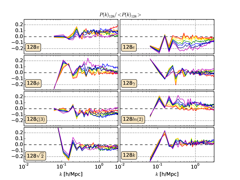
Figure 3: Simulations spectra of different realizations (dubbed: $\pi,~{}\phi,$$~{}\zeta(3),$$~{}\sqrt{2},~{}e,$$~{}\gamma,~{}ln(2),k$) in a 128 box, vs. their averages at 8 different redshifts ($z=3.00$ (red), $2.20$(orange), $1.5$(yellow), $1.00$(green), $0.7$(blue), $0.35$(indigo), $0.00$(violet)).

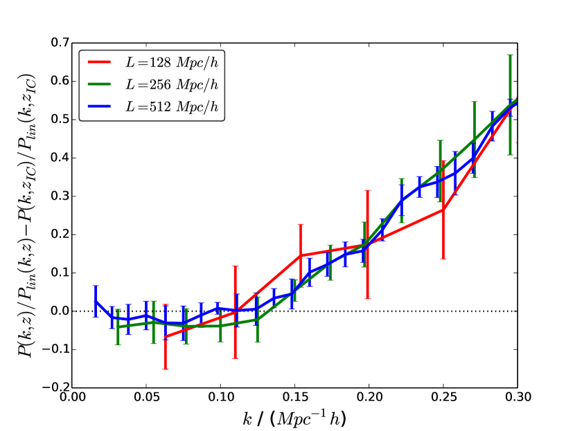
Figure 4: Average of spectra, after subtracting initial conditions from each of them, compared with linear growth.

In what follows we shall mostly report results obtained from simulations in 128 and 512$\,h^{-1}$Mpc boxes, with $n$ 1024 and 4096, respectively. Some results from 256$\,h^{-1}$Mpc box with $n=2048$ will only be cited in the final Section.

At low $k$ spectral values obtained form simulations still exhibit a significant dependence from the seed yielding Initial Conditions. This is clearly visible in Figure 3, referring to the 128$\,h^{-1}$Mpc box; here we make use of the spectra arising from the different seeds, dubbed: $\pi,~{}\phi,$$~{}\zeta(3),$$~{}\sqrt{2},~{}e,$$~{}\gamma,~{}ln(2),~{}k$; these symbols are preceded by the related box side in $\,h^{-1}$Mpc. For instance, for the box with 128 (512)$\,h^{-1}$Mpc aside, the simulations 128$e$ and 128$\gamma$ (512$\zeta(3)$ and 512$\sqrt{2}$) will be used. (When needed for graphic reasons these names are shortened, e.g., by omitting the box side or even by replacing $\zeta(3)$ or $\sqrt{2}$ by $\zeta$ or $\sqrt{}$.)

In Figure 3 we considered $P(k,z)$ up to $k\simeq 0.32\,h\,{\rm Mpc}^{-1}$ i.e., approximately, up to where spectral discreteness is visible on a logarithmic plot, when plotting $P(k)/\langle P(k)\rangle$; the denominator being an average among different realization spectra. This allows then us to appreciate that deviations from such average, due to the seed, are persistent at all subsequent $z$’s, starting from initial conditions.

Little use of $\langle P(k)\rangle$ will however be made in spectral analysis. Instead of using it, we shall rather refer to the actual realization closest to it. Then sample variance is estimated by comparing its spectra with those of the realization most distant from $\langle P(k)\rangle$ itself. According to the discussion in the previous Section, we shall neglect the discrepancy between a full ensemble average and the 8–average considered, as well as the discrepancies between the spectrum closest to $\langle P(k)\rangle$ and $\langle P(k)\rangle$ itself. These neglects will however allow us to treat the two simulations on the same footing.

The relevance of this approximation can be better appreciated by averaging among simulation octets, and comparing spectra from different box sizes, as is done in Figure 4. More precisely, in this Figure we consider the ratio $P(k,z)/P_{lin}(k,z)$, between the spectrum of simulations and the linear spectrum; we subtract from it the same ratio at $z_{IC}$, where IC were set; finally we average among the 8 realizations obtained from different seeds, for the 3 box sizes. This operation aims at minimizing the discreteness jumps which, as seen in the previous Figure 3 persist through redshifts, further smoothing the result by averaging among seeds. Error bars yield the sample variance at 1–$\sigma$.

The Figure allows us to confirm that the DC term we omitted in Initial Conditions implies a correction to variance substantially smaller than the expected discrepancy between estimated and actual sample variance. In fact, in the low–$k$ almost–linear range, although some lack of power of smaller boxes seems appreciable by eye, the sample variance at all $k$’s comfortably includes the zero point; furthermore, as soon as we enter the non–linear regime, the Figure shows the lack of any apparent trend indicating smaller box spectra to have less power than larger ones. On the contrary, in the initial mildly non–linear regime, the greatest fluctuation amplitudes are those obtained from the smallest box while, along the whole scale range shown, the greatest box average spectra never are the top ones (for an example of greater statistics making the DC term significant see, e.g., the plot in Figure 6 of Heitmann et al. (2010), analogous to Figure 4).

Let us now turn to the main aim of this work, detecting the impact of variance on shear spectra $C_{ij}(\ell)$. To do so we must treat each realization separately, ignoring other ones, by devising a recipe enabling us to use the spectra $P(k,z)$, obtained from each single realization, separately.

Each single spectrum, as derived from simulations, exhibits problems at small $k$, as we just appreciated, as well as large $k$ problems. The latter ones may be due either to lack of resolution –due to mass discreteness– or to numerical noise. In fact, the signal due to initial lattice can cover the $P(k)$ signal at high $z$’s if, as is usual, initial conditions are given on a grid rather than on a glass. The recipe to deal with this problems will be detailed in the next Subsection.

Large $k$ problems, however, are not so essential as those found at low–$k$ which, in turn, are quite different from those faced to build an average non–linear spectrum, at a given approximation level, as done, e.g., within the Coyote simulation suite (Heitmann et al., 2010). In fact, here we need to preserve the peculiarities deriving from each specific model realization in the assigned box, which are the essential feature whose impact on shear spectra we wish to gauge. In turn, at low $k$, each spectral point being derived by averaging over quite a limited number of realizations allowed inside the box size, significant jumps upwards and downwards, as those shown in Figure 3, are unavoidable.

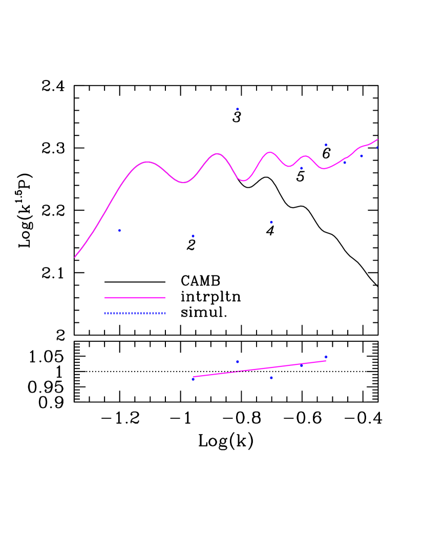
Figure 5: Low–$k$ interpolation between CAMB and numerical spectra for a box side $L=128\,h^{-1}$Mpc at $z=0~{}.$ The interpolatory curve in the upper frame is obtained by displacing the CAMB spectrum upwards, as soon as the linear interpolation of the ratio $\cal R$$(k_{i})$ (see text) exceeds unity. In the bottom plot $\cal R$$(k_{i})$ values and its linear interpolation are showed. All units are suitable powers of $h^{-1}$Mpc.

Figure 6: Points indicate the $k_{i}$ for which $P_{S}$ spectra are obtainable, when using a 128 or 512 $h^{-1}$Mpc box. Vertical lines indicate the limits of the 3 intervals where $P_{S}$ is interpolated with $P_{C}$, according to procedures outlined in the text. For the 128 (512) $h^{-1}$Mpc box the number of points in the two intervals is 6 (11).

The recipe to be used at low $k$ will also be discussed here below and detailed in the next Subsections. Let us soon outline that no use of perturbative expressions of mild spectral non–linearity will be made.

As a matter of fact, a large deal of work on this subject has been carried on along more than three decades, since Peebles (1980) book and Bernadeu et al (2002) review. Recent work (Crocce and Scoccimarro, 2006; Anselmi & Pietroni, 2012; Anselmi et al., 2014) shows that corrections to the linear spectrum approaching $1\,\%$ may be present up to $k\sim 0.003\,h$Mpc^-1, i.e. over scales $\sim 4$ times greater than those inspected by our greatest simulation box. More significantly, they extend perturbative techniques to $k$ values well beyond the BAO range, where non–linearity apparently dominates.

However, apart of the difficulty to extract from these results a handable parametric expression, such summation techniques apply to full ensemble averages. Possibly, their use could be effective to improve results obtained from averaging among a significant number of simulations. On the contrary, they are unlikely to apply to the results of single simulations.

Accordingly, we shall keep on the phenomenological side, and make use of expression bearing a purely analytical significance. Incidentally, when using our 512$\,h^{-1}$Mpc box, they univocally find that convergence on the linear results is attained for $\log(k/h{\rm Mpc})^{-1})\simeq-1.2,$ in agreement with Matsubara (2008) and Carlson et al. (2009).

The basic steps of our technique are as follows: we first interpolate the linear spectra to obtain their values $P_{C}(k_{i})$ at the very $k_{i}$’s where the simulation spectrum $P_{S}(k_{i})$ is calculated. We then fit the ratio

$${\cal R}(k_{i})=\log[P_{S}(k_{i})]/\log[P_{C}(k_{i})]$$ (6)

with a curve growing linearly with $k$, for the first few points, allowing for a more detailed correction after a few of them. We do so we neglect the first point $k_{1}$ and refer to different numbers of $k_{i}$’s for the different box sizes, although selecting them through fixed rules. In order to be more precise, let us now distinguish between different box sizes.

3.1 Simulations in 128$\,h^{-1}$Mpc box

The hardest case is the 128³ particle simulations, for which we provide some more details. In this case we start from the $k_{i}$ values with $i$ from 2 to 6 (five values) and determine the $P$ and $Q$ coefficient minimizing the expression

$$diff=\sum_{i}\left[(P+Qk_{i})/{\cal R}(k_{i})-1\right]^{2}~{},$$ (7)

adding a specific condition, soon specified here below. We then fit the simulation spectrum with the expression

$$\log[P_{fit}(k)]=\log[P_{C}(k)]\times(P+Qk)$$ (8)

for all $k$ values where it exceeds $\log[P_{C}]$. The specific condition outlined here above, is that the spectrum must however meet the linear spectrum at any $k$ smaller than a suitable $\bar{k}$. The point is not only that non–linear effects are surely (almost) absent below such suitable $k$ value, but that simulations cannot provide information on possible (residual) non–linearities for length scales $2\pi/k$ too close to the box side. For our box side $L_{box}=128\,h^{-1}$Mpc, we then take $\bar{k}=0.1\,h\,$Mpc^-1 (yielding a length scale $\sim L_{box}/2)~{}.$

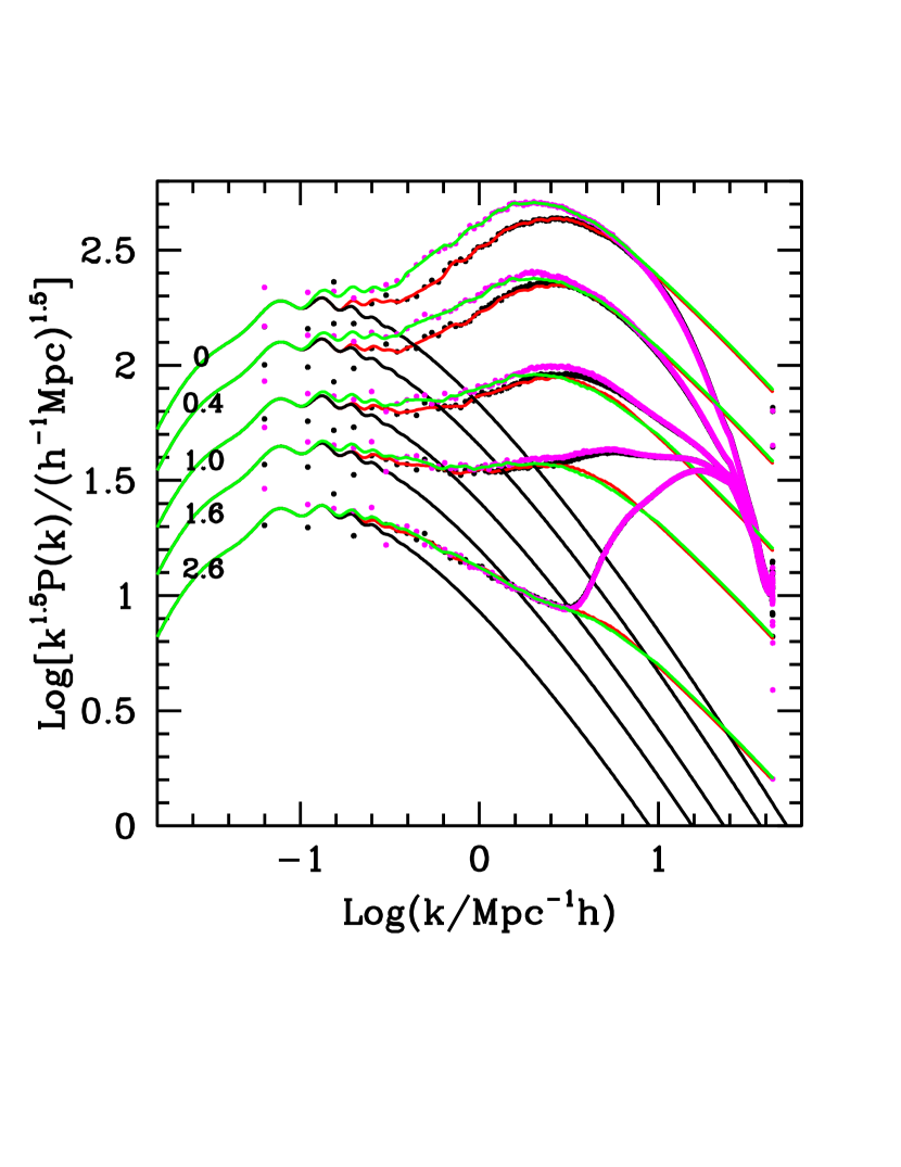
Figure 7: Spectra obtained from simulations in a box with $L=128\,h^{-1}$Mpc aside, interpolated with linear CAMB outputs. The main feature shown in this figure is the significant discrepancy between the two seeds, dubbed $128\gamma$ (closest to average) and $128e$ (farthest from average and smaller from it). Magenta and black points, respectively, yield the resulting simulation outputs. From CAMB and them we derive the green and red spectra (also respectively), as explained in the text.

Figure 8: Ratio between the spectra deriving from the seeds $128e$ & $128\gamma$, at the redshifts indicated in the frames. The top discrepancy shown, at $z=0$ and $k/(h\,{\rm Mpc}^{-1})\sim 0.65$, is $\simeq 37.4\,\%$.

Fig. 5 gives more details and shows the results of this operation. In the upper panel we show the overall interpolation (magenta curve). In the lower panel we show the ratios ${\cal R}(k_{i})$ and their linear interpolation $P+Qk$, to be used where it exceeds unity (the magenta line). This technique is meant to preserve the BAO structure outlined by the linear algorithm, just suitably shifting it upwards, according to the requirements coming from the first $k_{i}$ values in the simulation.

We then consider 6 more points and allow for a correction to $P+Qk$ by a term $R(k-k_{6})^{\alpha}$, $R$ and $\alpha$ being again determined through a l.s. fit. This is meant to allow a progressive rise of the spectral steepness, following the gradual incoming on non linear dynamics. Accordingly, this approach must be gradually modified at higher $z$, when non linear dynamics does not yet affect smaller $k_{i}$’s. As a matter of fact, at fairly large $z$ values, not only the $P$ and $Q$ coefficients may turn out to be quite small, but there may be no need of power law corrections. Then, if $P_{fit}(k)$ exceeds $P_{S}(k)$ in two –or more– $k_{i}$ points ($7\leq i\leq 12$), we shall deal with these points as we do with those above the 12–th, and is described below.

In Figure 6 we show the limits on the $k$ axis of the two above intervals, both in this case and for the forthcoming 512$\,h^{-1}$Mpc box.

Starting from $k_{n}$ with $n\geq 13$, we then perform a Savitski–Golay (SG) interpolation. More precisely, we consider $2p$ values $k_{n\pm j}$ ($j=1,..,p$), plus $k_{n}$ itself, and interpolate them to obtain $2p+1$ equispaced points on a $\log k$ scale, with extremes in $k_{n\pm p}$. In this way we work out a spectral value for $k^{\prime}_{n}=10^{[\log(k_{n-p})+\log(k_{n+p})]/2}$, a point quite close to $k_{n}$ but not coinciding with it. The values of $p$ go from 4 to 8, suitably increasing towards greater $k_{n}$ values.

Before passing to briefly describing the large–$k$ treatment, let us still outline that the same treatments are reserved to all seeds. In particular, when $P_{fit}(k)$ exceeds $P_{S}(k)$ for almost 2 $k_{i}$ points ($7\leq i\leq 12$) in one simulation, we start operating a SG interpolation for all of them.

As far as large–$k$ and low $z$ are concerned, resolution problems begin to damp the spectrum at $k/h\,{\rm Mpc}^{-1}\sim 3\,$. On the contrary, at large $z$, numerical noise cancels spectral features; e.g., at $z=2.8$, this occurs at $k\sim 5\,.$

The problems we meet, therefore, concern a range where physical signal cannot be predicted by using gravitation only. Accordingly, our treatment is meant just to test sample variance in shear spectra; as any previous weak lensing treatment, based on N–body simulations only, the values found for the shear spectra start to be biased as soon as $\ell>\sim 500$ (see also Figure 12, herebelow).

Accordingly, we implement an algorithm detecting two possible spectral anomalies: (i) Non linear spectra decreasing more rapidly than CAMB linear spectra $\times k^{\alpha}$, when $k$ increases (the results are obtained with $\alpha=0.8$, in rough agreement with a generic trend visible also in (Smith et al., 2003)). (ii) Spectra exhibiting an increasing steepness, well after non–linearity has onset.

In both cases, our algorithm gradually replaces numerical spectra with curves parallel to the linear CAMB spectrum $\times k^{\alpha}$. Here again, we abandon the numerical spectrum at the same $k$ values for all seeds.

In Fig. 7 we show the results of these operations for 2 simulations in boxes of side $L=128\,h^{-1}$Mpc. These simulations are dubbed $128\gamma$ and $128e$ in Figure 3, and are those closest and farthest from average, respectively.

The size of the discrepancy between these simulations can be further appreciated in Figure 8, where we plot the ratio between the spectra obtained from the two seeds, and its low $z$ evolution. Its top value, estimated by considering averages among $N$ points ($N=6$) amounts to 37.4$\,\%~{}.$

3.2 Simulations in 512$\,h^{-1}$Mpc box

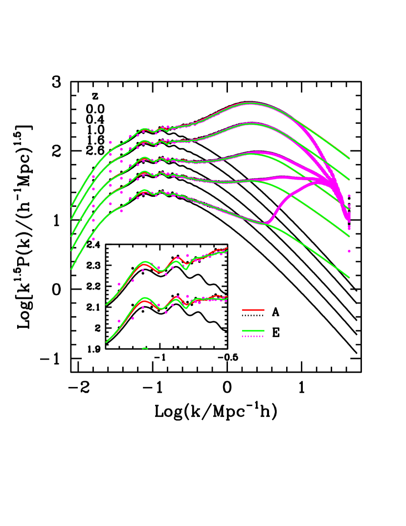
Figure 9: Spectra obtained from simulations in a box with $L=512\,h^{-1}$Mpc aside, interpolated with linear CAMB outputs. The seeds closest and farthest from (mostly greater than) average are those dubbed $512\sqrt{2}$ and $512\zeta(3)$. Here again, spectra in black are CAMB outputs. Black and magenta points yield actual simulation outputs. From CAMB and them we derive the red and green spectra (respectively), as explained in the text. Notice also the significant spectral discrepancy occuring at small $k$ values, magnified in the inner box; for a significant $k$–interval, its sign is opposite in respect to the main trend, as the very “points” of spectrum A, which lay above the “points” of spectrum E.

Figure 10: Ratio between the spectra from the seeds $512\sqrt{2}$ & $512\zeta(3)$, at the redshifts indicated in the frames. Notice the ordinate scale expanded in respect to the analogous Figure 7. Jumps at low $k$ have alternate signs and arise in the linear/non–linear connection region where the box still contains a limited number of realizations. As explained in the text, they have a lesser impact than the steady excess of $P_{\sqrt{2}}$ on $P_{\zeta(3)}$ at greater $k$ values.

The same tecnique used for the smaller box is now extended to this wider box, to allow a linear/non–linear connection. In Figure 6 we compare the range of $k$ values used in the two cases. The number of “points” used in the low–$k$ intervals is now 11. Tries performed with close numbers of points (e.g. 10 or 12) yield greater fitting residuals.

Figure 9 is then analogous to Fig. 7, although spectral “points” here extend down to smaller $k$ values, just marginally non–linear. These points are indeed obtained by averaging over a limited number or realization, so that sample variance is large and partially hides non–linearity itself. In the inner box this scale range is magnified, also showing the smoothness of the linear/non–linear interpolated red and green curves, however crossing a few times.

The overall situation is more clearly outlined by Figure 10, analogous to Figure 8; notice however the reduced range of the ordinates. Here we clearly distinguish the effects due to the limited number of realizations at low $k$, which persist through all $z$ without an appreciable amplitude growth, from the actual sample variance between the two seeds, in the $k$ interval (-0.6 – +0.7), steadily growing because of non–linearity: at $z=2.6$ the spectral ratio is still $\sim 1\,\%$; at $z=0$ it finally reaches $5.32\,\%$ (evaluated with the same criterion as from Figure 8).

4 Tomographic windows

Let us now investigate how these variance effects transfer from fluctuation to shear spectra. To do so, let us build the needed tomographic windows, by starting from the expression of the background metric reading

$$ds^{2}=a^{2}(\tau)[d\tau^{2}-d\lambda^{2}]~{},$$ (9)

$d\lambda$ being the comoving space element, while $\tau$ is the conformal time; both are measured in $h^{-1}$Mpc. Let then $a(\tau)=1/(1+z)$ be the scale factor, $z$ being the redshift. Let us further define the conformal time delay at redshift $z$

$$u(z)=\tau_{0}-\tau(z)~{},$$ (10)

$\tau_{0}$ being the present conformal time, and the inverse function $z(u)$.

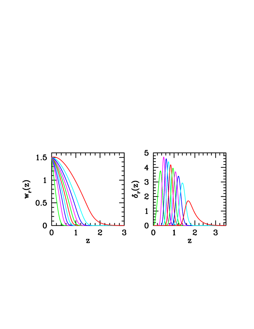
Figure 11: Expected distributions on redshift of galaxies belonging to different bands (l.h.s.) and related filters (r.h.s.). Upper (lower) panel refers to the 5 (10) band case.

Galaxies observed in a unit solid angle are then assumed to have a redshift distribution

$$n(z)={d^{2}N\over d\Omega\,dz}={\cal C}\times\bigg{(}{z\over z_{0}}\bigg{)}^{A}\exp\bigg{[}-\left(z\over z_{0}\right)^{B}\bigg{]}$$ (11)

with $A=2$, $B=1.5$ so that

$${\cal C}={B\over\left[z_{0}\Gamma\left(A+1\over B\right)\right]}={1.5\over z_{0}}$$ (12)

(here $z_{0}=z_{m}/1.412$ while the median redshift $z_{m}=0.9~{}$, in agreement with Euclid specifications).

These galaxies will be shared in $N=5$ or 10 redshift bands, whose limits $z_{r}$ are selected so that they contain equal galaxy numbers. For large galaxy sets, photometric redshifts only are expected to be available and, to evaluate the expected distribution on redshift for the $r$–th band galaxies, we apply the filters

$$\Pi_{r}(z)=\int_{z_{r}}^{z_{r+1}}dz^{\prime}~{}{\exp\left[-{(z-z^{\prime})^{2}\over 2\,\sigma^{2}(z)}\right]\over\sqrt{2\pi}~{}\sigma(z)}~{}=~{}{1\over 2}\left[{\rm Erf}\left(z_{r+1}-z\over\sqrt{2}\sigma(z)\right)-{\rm Erf}\left[z_{r}-z\over\sqrt{2}\sigma(z)\right]\right]$$ (13)

to $n(z)$. In this way we obtain the distributions

$$D_{r}(z)=n(z)\Pi_{r}(z)$$ (14)

whose integrals are $\simeq 1/N$. In this work we shall take $\sigma(z)=0.05~{}(1+z)$, coherently with Euclid expectations (Amendola et al. (2013), see also Casarini et al. (2011)); the distributions $D_{r}$, when normalized to unity, are then dubbed $\delta_{r}$ . They are used to define the window functions

$$w_{r}(u)={3\over 2}[1+z(u)]\int_{u}^{\infty}du^{\prime}~{}\delta_{r}(u^{\prime})~{}{u^{\prime}-u\over u^{\prime}}~{},$$ (15)

also shown in Figure 11.

5 Shear spectra

Shear spectra are then related to the power spectra $P_{\delta}(k,u)\equiv P[k,z(u)]$, through the relation

$$C_{ij}(\ell)=(H_{0}^{2}\Omega_{0m})^{2}\int_{0}^{\tau_{0}}du~{}w_{i}(u)\,w_{j}(u)~{}P_{\delta}(\ell/u,u)~{}.$$ (16)

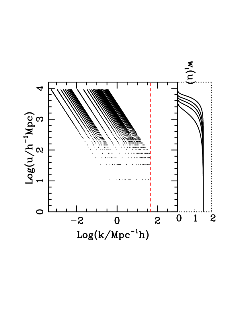
Figure 12: Integration patterns for a number of $\ell$ values between 5 and 3300. Points indicated are those used in the case of Riemann integration with 400 points (yielding results visually indistinguishable from those with more points). The red dashed line is the limit beyond which (just a few) integrand values are to be obtained by interpolation. In the right frame we show the patterns of window functions $w_{i}(u)$, in the case of 5 bands.

Integrals are performed by using a modified Riemann algorithm with 10000 equispaced integration points $u_{\alpha}$ up to $u_{top}\simeq 9000$ (instead of $\tau_{0}$). Integration results are visually indistinguishable from those obtained with just 400 points and, for this case, in Figure 12 we show the points selected on the $\log k$–$\log u$ plane, for a subsample of $\ell$ values, lying along tilted straight lines.

Integration therefore requires interpolation of $w_{j}(u)$ at $u_{\alpha}$ and of $P_{\delta}$, first along $k$ and then again along $u$. A number of cases is then considered: for 5 and 10 tomographic bands; for simulations in 128(, 256) and 512$\,h^{-1}$Mpc boxes, with resolution pushed up to 1024(, 2048) and 4096 points, respectively; for those 2 seeds, selected for each box size, for being closest and farthest from average.

5.1 Shear spectra from simulations in the 128$\,h^{-1}$Mpc box

In Figure 13 we plot the shear spectra obtained from the fluctuation spectra arising from the seed $128\gamma$, in the case of a 5 band tomography. Aside of them we also show (black dotted curves) the spectra obtainable from $128e$. In Figure 14 we then show the spectra for a 10 band tomography obtained from $128e$.

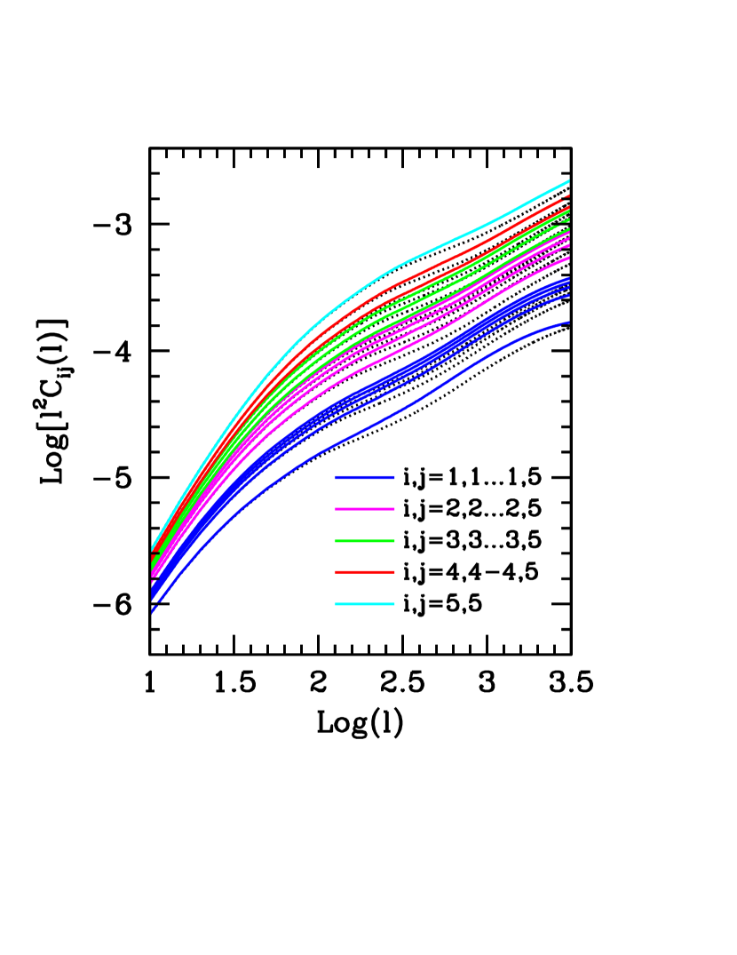
Figure 13: Solid lines yield the shear spectra $C_{ij}(\ell)$ for the 128$\gamma$ seed, in the case of a 5 band tomography. Colors account for _i,j indices. Almost overlapped to them we also plot the spectra obtained from the $128e$ seed (black dotted curves), so outlining the significant discrepances between the two seeds.

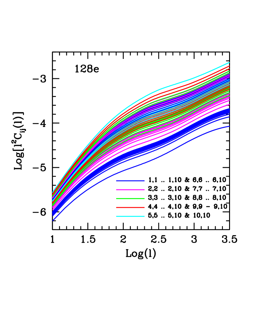
Figure 14: Shear spectra $C_{ij}(\ell)$ for the 128$e$ seed, in the case of a 10 band tomography.

The discrepancy between seeds is better visible in Figures 15 and 16, for the 5 and 10 band cases, respectively.

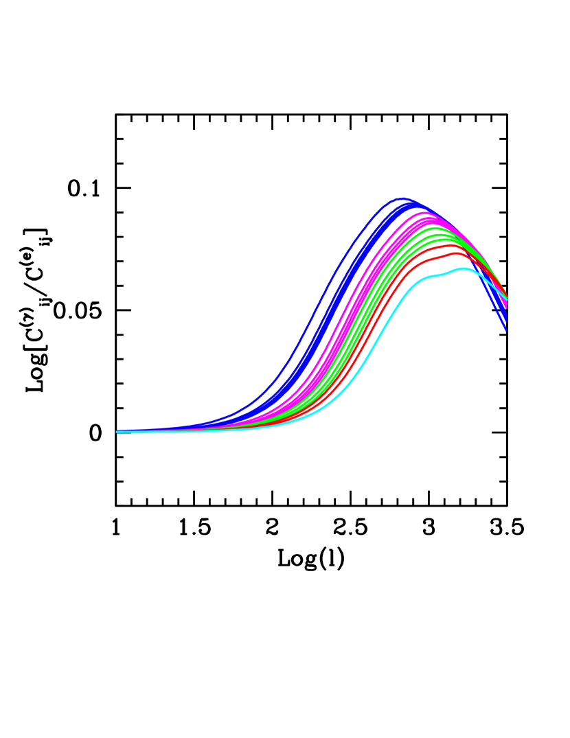
Figure 15: Ratio between spectra obtained from the 128$\gamma$ and 128$e$ seeds, in the case of a 5 band tomography .

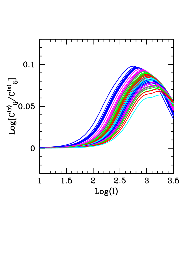
Figure 16: As previous Figure for a 10 band tomography .

These plots allow us 2 comments: (i) The shear spectra discrepancy is substantially independent from the number of bands and reaches $24.7\,\%$ for $C_{11}$ for a 5 band tomography; this top discrepancy is estimated similarly to $P_{\delta}$ spectra, by averaging over $\ell$ with $N=10$. (ii) If we remind that shear spectra are obtained by integrating over redshift, so including contributions from $P_{\delta}$ up to $z\sim 2$, we appreciate that no substantial decrement of spectral discrepancy occurs, when passing from fluctuation to shear spectra.

5.2 Shear spectra from simulations in the 512$\,h^{-1}$Mpc box

Discrepancies, as expected, are significantly smaller when a greater simulation box is used. In Figure 17 we plot shear spectra obtained from the 512$\zeta(3)$ seed, in the cases of a 5 band tomography. As in the smaller box case, we overlap these spectra with those obtainable from the 512$\sqrt{2}$ seed, which is the most distant from average and, in this case, exceeds average. Discrepancies, however, are quite hard to be perceived in this way.

In Figure 18 we then plot shear spectra in the case of a 10 band tomography, as obtainable from the 512$\sqrt{2}$ seed.

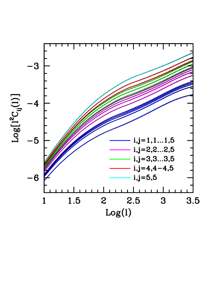
Figure 17: Shear spectra from the 512$\zeta(3)$ seed, in the case of a 5 band tomography. Black dotted curves yield the spectra as obtainable from the 512$\sqrt{2}$ seed, however hardly distinguishable, in this case.

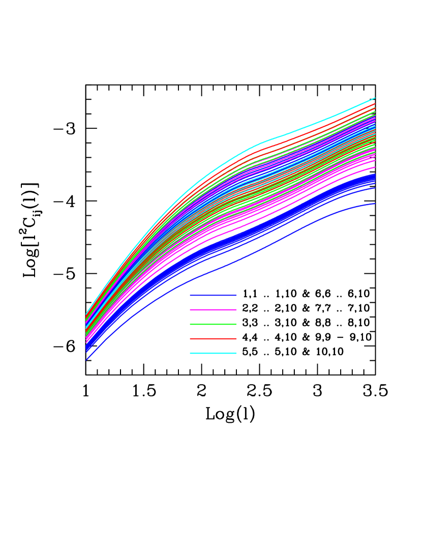
Figure 18: Shear spectra from the 512$\sqrt{2}$ seed, in the case of a 10 band tomography.

In Figures 19 and 20, we finally plot the ratios between the shear spectra obtained from the simulations 512$\zeta(3)$ and 512$\sqrt{2}$ in the cases of 5 and 10 bands.

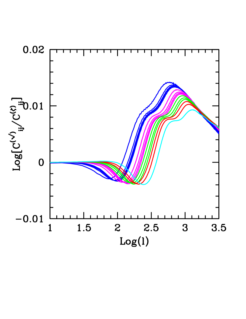
Figure 19: Ratio between spectra obtained from the 512$\sqrt{3}$ and 512$\zeta(3)$ seeds, in the case of a 5 band tomography .

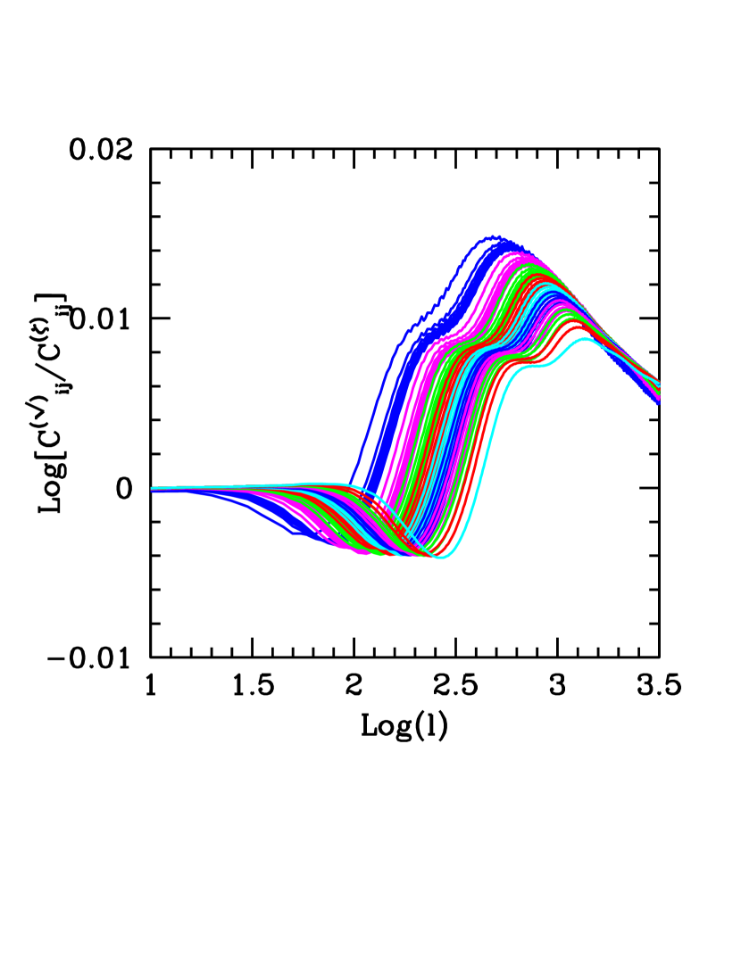
Figure 20: As previous Figure, in the case of a 10 band tomography .

Tiny oscillations in the curve arise from residual oscillations of $P_{\delta}$, visible here because of the reduced amplitude of the overall ratio; when comparing Figures 19 & 20 with Figures 15 & 16, take also notice of the reduced range of the ordinates.

Once again we appreciate that discrepancies are almost independent from the number of tomographic bands and their top value is $\sim 3.32\,\%$.

Let us finally outline the peculiar feature that ratios exhibit at low $\ell$, where they become less than unity. As a matter of fact, at low $k$, the very ratio between $P_{\delta}$ spectra exhibits significant oscillations about unity (see Figure 10), smeared out by the integrals (16), yielding the prevealing contribution, in a direction opposite to the main trend at greater $k$’s.

This kind of peculiarities become more and more significant as we go to greater boxes and, consequently, also to smaller bulk discrepancies. If making use of different seeds, for which such bulk discrepancy is however smaller, we find similar anomalies. The essential point is that they fall in a region necessarily separate from that allowing us the basic estimate of top discrepancies.

6 Discussion and conclusions

This paper makes use of sets of $\Lambda$CDM N–body simulations to investigate sample variance, in view of the possible use of ad–hoc simulations to fit data exhibiting evident deviation from GR or other peculiar effects due to the nature of the dark components.

Such evidence could derive from the analysis of weak lensing data. Accordingly, the effects of sample variance on tomographic shear spectra are also inspected.

Our analysis is based on 8 $N$–body simulations in boxes of increasing side $L$. According to simple probabilistic arguments, the spread between their results approaches $\sim 1.5\,\sigma$’s. Experiments in progress plan to achieve a precision $\sim 1\,\%$; accordingly, the size of the simulation box and the related resolution should enable us to reach the same precision, at least.

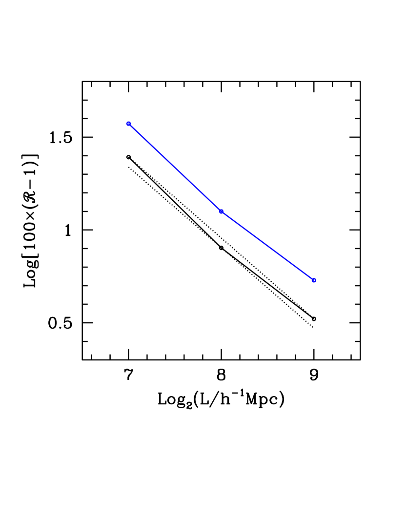
Figure 21: Top ratio ${\cal R}_{max}$, between fluctuation or shear spectra (in blue or black, respectively). In the latter case values are for a 10 band tomography, although the dependence on the band number is almost negligible.

In Figure 21 we then plot the maximum discrepancies between the “most distant” realizations considered as a function of the box side. The $k$ values where they arise lay in the spectral region where $k$ discreteness is still relevant. It is so, in spite of their being damped by our procedure, using sets of simulations points to “bend” linear spectra, so to account for the rise of non–linearity. More precisely, in Figure 21, we consider the ratios ${\cal R}=\left|\log[P_{\delta}^{(1)}(z=0)]/P_{\delta}^{(2)}(z=0)]\right|$ (in blue) or $\left|\log(C_{ij}^{(1)}/C_{ij}^{(2)})\right|$ (in black); apices refer to the 2 seeds considered (closest and farthest from average) for each box side. Such ratio overcome the unity by an amount which, multiplied by 100, yields the percent discrepancy. This surely yields values greater than an estimate referring to spectral covariance, based on averaging among discrepancies, as was done by previous authors (see, in particular, Takahashi et al. (2009)). In Figure 21 we show that the percent discrepancy between the most distant realizations decreases almost linearly with the box side, being cut by a factor $\sim 0.35$–0.45 when the side doubles. This is true both for $P_{\delta}(k)$ and $C_{ij}(\ell)$.

The decrease is surely expected, as the number of realizations considered within each box increases with the box size. An analogous decrease is shown, e.g., in Fig. (12) of Takahashi et al. (2009), although they plot spectral covariance and their increase in the realization number arises from increasing the number of equal size boxes taken, within a very large number of independent simulation boxes.

Being wider, however, the size of our dependence on the box side is safer, in respect to varying I.C. in a set of 8 simulation boxes. An estimate of such residual dependence is obtainable from the apparent deviation of the $L$ dependence from linear. In Figure 21 and for the $C_{ij}$ discrepancies, two dashed lines frame the expected interval for a linear behavior. If we assume that the uncertainty of each estimate is set by the width of such interval, we find $\sim 13\,\%$. Similarly, for $P(k)$, we find $\sim 15\,\%$.

If we extrapolate the linear behavior to seek where realization discrepancies within a 8 box set, defined according to our criterion, are expected to lay below $1\,\%$, we find a box side in the range $1300$–$1700\,h^{-1}$Mpc, within the allowed range of slopes. It is also clear that discrepancy estimates do not depend just on box size, but also on mass and force resolution. Our choice is however a typical one, meant to optimize the results of the numerical effort.

This lead us to conclude that a set of 8 simulations in a box with 512$\,h^{-1}$Mpc aside is still insufficient to provide a unbiased test for any model, if the precision level wanted ranges around $1\,\%~{};$ such aim might be however approached with a box side $\sim 3$–4 times greater, keeping at the same resolution level and, therefore, accordingly increasing the dynamical range.

As many reseachers previously did, e.g. to provide spectral estimators (see, e.g., Heitmann et al. (2010, 2013); Lawrence et al. (2014)), one could prefere to run a large number of simulations in smaller boxes, aiming to examine the same number of realizations without expanding so far the required dynamical range. For instance, one could replace the 8 boxes $\sim 1700\,h^{-1}$Mpc aside, with $\sim 300$ boxes with $\sim 500\,h^{-1}$Mpc aside or $\sim 60$–70 realizations in boxes with $\sim 800\,h^{-1}$Mpc aside.

A first point to outline is then that including the impact of DC modes, i.e., of wavelength wider than the simulation box, marginally irrelevant when the statistics is limited to 8 boxes, would then become indispensable.

Changing the box size, however, bears a further consequence, as the density of values along the $k$ axis is bound to vary. Changing the discrete mode set in the simulation will then affect the covariance of the 3–D mass density. In turn, this affects the covariance of the mass density power spectrum. These mode–coupling effects were first outlined by Hamilton, Rimes & Scoccimarro (2006) (see also recent results by Takada & Hu (2013) and Li, Hu & Takada (2014)).

Sample variance is directly connected to that, so that we cannot restrict ourselves to barely counting the number of realizations as a function of the overall volume. This point is to be borne in mind and carefully weighted when a further effort to attain $C_{ij}$ prediction at precision level $\cal O$$(1\,\%)$ were deployed.

Acknowledgments

An anonymous referee is to be thanked, in particular for outlining us the effects on covariance of changing the box size. SAB acknowledges the support of the Italian CIFS. LC and OFP are grateful to CNPq (Brazil) and Fapes (Brazil) for partial financial support. This work has made use of the computing facilities of the Laboratory of Astroinformatics (IAG/USP, NAT/Unicsul), whose purchase was made possible by the Brazilian agency FAPESP (2009/54006-4) and the INCT-A.

References

- Albrecht et al. (2006) Albrecht, A., Bernstein, G., Cahn, R., Freedman, W. L., Hewitt, J., Hu, W., Huth, J., Kamionkowski, M., Kolb, E. W., Knox, L. et al., 2006, preprint astro-ph/0609591
- Alimi et al (2010) Alimi J. M., Füzfa A., Boucher V., Rasera, Y., Courtin, J., Corasaniti ,P. S., 2010, MNRAS, 401, 775
- Amendola et al. (2000) Amendola, L., 2000, Phys. Rev. D, 62, 643511
- Amendola et al. (2002) Amendola, L., Tocchini-Valentini, D., 2002, Phys. Rev. D, 66, 043528
- Amendola et al. (2003) Amendola, L., Quercellini, C., Tocchini-Valentini D., Pasqui A., 2003, ApJ Lett., 583, L53
- Amendola (2004) Amendola, L., 2004, Phys. Rev. D 69, 103524
- Amendola et al. (2007) Amendola, L. et al., 2013, Living Rev. Relat., 16,6
- Amendola et al. (2013) Amendola, L., Polarski, D., & Tsujikawa, S., 2007, Phys. Rev. Lett. 98, 131302
- Angulo et al. (2014) Angulo R. E., Springel V., White S.D.M., Jenkins A., Baugh C.M., Frenk C.S. (2012) MNRAS 426, 2335
- Anselmi & Pietroni (2012) Anselmi S., Pietroni M. (2012) JCAP 12, 13
- Anselmi et al. (2014) Anselmi, S., Lopez Necir, D. & Pietroni, M. (2012) JCAP 7, 13
- Bacon et al. (2000) Bacon, J., Refregier, A. R., & Ellis, R. S., 2000, MNRAS, 318, 625
- Baldi et al. (2010) Baldi M., Pettorino V., Robbers G. & Springel V., 2011, MNRAS 403, 1684
- Bertshinger (2001) Bertschinger, E., 2001, ApJS, 137, 1
- Blazek et al. (2012) Blazek, J., Mandelbaum, R., Seljak, E. & Nakajima, R., arXiv:1204.2264
- Brax & Martin (2000) Brax, P., & Martin, J. 2000, Phys. Rev. D, 61, 103502
- Capozziello et al. (2006) Capozziello, S., Nojiri, S., Odintsov, S. D., & Troisi, A., 2006, Phys. Lett. B 639, 135
- Casarini et al. (2009) Casarini, L., Macció, A. V., Bonometto, S. A., 2009, JCAP 3, 14
- Casarini (2010a) Casarini, L., 2010, JCAP, 08, 5
- Casarini (2010b) Casarini, L., 2010, NewA, 15, 57
- Casarini et al. (2011) Casarini, L., La Vacca, G., Amendola, L., Bonometto, S. A., Macció, A. V., 2011, JCAP, 3, 26
- Casarini et al. (2012) Casarini, L., Bonometto, S.A., Borgani, S., Dolag, K., Murante, G., Mezzetti, M., Tornatore, L., La Vacca G., 2012, AA 542, 126
- Crocce and Scoccimarro (2006) Crocce, M., Scoccimarro, R. (2006) Phys.Rev. D, 73, 063520
- Das et al. (2005) Das, S., Corasaniti, P. S., Khoury, J., 2006, Phys. Rev. D, 73, 083509
- Ellis et al. (1989) Ellis, J., Kalara, S., Olive, K. A., & Wetterich, C., 1989, Phys. Lett. B, 228, 264
- Heitmann et al. (2010) Heitmann, K., White, M., Wagner, C., Habib, S., & Higdon, D., 2010, ApJ, 715, 104
- Heitmann et al. (2013) Heitmann K., Lawrence E., Kwan J., Habib S., and Higdon D., 2014, ApJ, 780, 111
- Hu (2002) Hu, W., 2002, Phys. Rev. D 65, 023003
- Kaiser et al. (2000) Kaiser, N., Wilson, G., & Luppino, G. A., preprint astro-ph/0003338
- Carlson et al. (2009) Carlson, J, White, M, Padmanabhan, N, Phys. Rev. D, 80, 043531
- Hamilton, Rimes & Scoccimarro (2006) Hamilton A.J.S., Rimes C.D., Scoccimarro R., 2006, MNRAS 371, 1188
- Heitmann et al. (2014) Heitmann K., Lawrence E., Kwan J., Habib S., Higdon D., 2014, ApJ 780, 111
- Klypin & Holtzmann (1997) Klypin, A., & Holtzman, J., 1997, preprint astro-ph/9712217
- Klypin et al. (2003) Klypin, A., Macció, A. V., Mainini, R., Bonometto, S. A., 2003, ApJ 599, 31
- Klypin et al. (2011) Klypin, A., Trujillo-Gomez, S., Primack, J., 2011, ApJ, 740, 102
- La Vacca & Colombo (2008) La Vacca, G., & Colombo, L. P. L., 2008, JCAP, 0804, 007
- Lawrence et al. (2014) Lawrence E., Heitmann K., Khite M., Higdon D., Wagner C., Habib S., Williams B., 2009, ApJ 705, 156 & 2010, ApJ 713, 1322
- Lewis & Bridle (2002) Lewis, A., & Bridle, S., 2002, Phys. Re v. D66, 103511
- Li, Hu & Takada (2014) Li Y., Hu W., Takada M., 2014, Ph.Rev.D 89, 083519
- Maccio’ et al. (2004) Macció, A. V., Quercellini, C., Mainini, R., Amendola, L., Bonometto, S. A., 2004, Phys. Rev. D, 69, 123516
- Matsubara (2008) Matsubara, T., 2008, Phys Rev D, 78, 083519
- Mezzetti et al. (2012) Mezzetti, M., Bonometto, S. A., Casarini, L., Murante, G., 2012, JCAP, 06, 5
- Peacock et al. (2006) Peacock, J. A., Schneider, P., Efstathiou, G., Ellis, J. R., Leibundgut, B., Lilly, S. J., Mellier Y., 2006, preprint astro-ph/0610906
- Planck collaboration (2013) Planck Collaboration, 2013, preprint arXiv:1311.1657
- Puchwein et al. (2013) Puchwein E., Baldi B. & Springel V., 2013, arXiv:1307.5065
- Ratra & Peebles (1988) Ratra, B., & Peebles, P. J. E. 1988, Phys. Rev. D, 37, 3406
- Sirko (2005) Sirko, E., 2005, ApJ, 634, 728
- Li et al. (2014) Li Y., Hu W., & Takada, M., 2014, Phys.Rev. D, 90, 103530
- Smith et al. (2003) Smith, R. E., et al., 2003, MNRAS, 341, 1311
- Stadel (2001) Stadel, J.G., 2001, PhD thesis, University of Washington
- Springel et al (2005) Springel, V. & et al, 2005, Nature, 435, 629
- Takada & Hu (2013) Takada M. & Hu W., 2013, Phys.Rev. D, 87, 123504
- Takahashi et al. (2009) Takahashi R., Yoshida N., Takada M., Matsubara T., Sugiyama N., Kayo I., Nishizawa A.J., Nishimichi T., Saito S., Taruya A., 2009, ApJ 700, 479
- Van Waerbeke et al. (2000) Van Waerbeke et al., 2000, A&A, 358, 30
- Wetterich (1995) Wetterich, C., 1995, A&A, 301, 321
- Wittman et al. (2000) Wittman, D. M. et al., 2000, Nature, 405, 143