Energy Spectrum of Buoyancy-Driven Turbulence

Abstract

Using high-resolution direct numerical simulation and arguments based on the kinetic energy flux $\Pi_{u}$, we demonstrate that for stably stratified flows, the kinetic energy spectrum $E_{u}(k)\sim k^{-11/5}$, the entropy spectrum $E_{\theta}(k)\sim k^{-7/5}$, and $\Pi_{u}(k)\sim k^{-4/5}$, consistent with the Bolgiano-Obukhov scaling. This scaling arises due to the conversion of kinetic energy to the potential energy by buoyancy. For weaker buoyancy, this conversion is weak, hence $E_{u}(k)$ follows Kolmogorov’s spectrum with a constant energy flux. For Rayleigh Bénard convection, we show that the energy supply rate by buoyancy is positive, which leads to an increasing $\Pi_{u}(k)$ with $k$, thus ruling out Bolgiano-Obukhov scaling for the convective turbulence. Our numerical results show that convective turbulence for unit Prandt number exhibits a constant $\Pi_{u}(k)$ and $E_{u}(k)\sim k^{-5/3}$ for a narrow band of wavenumbers.

I Introduction

Buoyancy or density gradients drive flows in the atmosphere and interiors of planets and stars, as well as in electronic devices and industrial appliances like heat exchangers, boilers, etc. Accordingly, scientists (including geo-, astro-, atmospheric- and solar physicists) and engineers have been studying buoyancy-driven flows for more than a century. An important unsolved problem in this field is how to quantify the spectra and fluxes of kinetic energy and entropy ($u^{2}/2$ and $\theta^{2}/2$ respectively, where $\mathbf{u}$ and $\theta$ are the velocity and temperature fluctuations) of buoyancy-driven flows Siggia (1994); Lohse and Xia (2010). In this paper, we will study these quantities and respective nonlinear fluxes using direct numerical simulations, and show that the kinetic energy (KE) spectrum differs from Kolmogorov’s theory when buoyancy is strong.

Flows driven by buoyancy can be classified in two categories: (a) convective flows in which hotter and lighter fluid at the bottom rises, while colder and heavier fluid at the top comes down; (b) stably stratified flows in which lighter fluid rests above heavier fluid. The convective flows are unstable; but the stably stratified flows are stable, hence their fluctuations vanish over time. Therefore, a steady state of a stably stratified flow is achieved only when it is driven by an external force. Even though both types of flows are driven by density gradients, the properties of such flows are quite different, which we decipher using quantitative analysis of energy flux and energy supply rate by buoyancy.

For a stably stratified flow, Bolgiano Bolgiano (1959) and Obukhov Obukhov (1959) first proposed a phenomenology, according to which the KE flux $\Pi_{u}$ of a stably stratified flow is depleted at different length scales due to a conversion of KE to “potential energy” via buoyancy ($u_{z}\theta$). As a result, $\Pi_{u}(k)$ decreases with wavenumber, and the energy spectrum is steeper than that prediced by Kolmogorov theory $(E(k)\sim k^{-5/3}$, where $k$ is the wavenumber); we refer to the above as BO phenomenology or scaling. According to this phenomenology, for $k<k_{B}$, where $k_{B}$ is the Bolgiano wavenumber Bolgiano (1959), the KE spectrum $E_{u}(k)$, entropy spectrum $E_{\theta}(k)$, $\Pi_{u}$, and entropy flux $\Pi_{\theta}$ are:

$$E_{u}(k) = c_{1}(\alpha^{2}g^{2}\epsilon_{\theta})^{2/5}k^{-11/5},$$ (1)

$$E_{\theta}(k) = c_{2}(\alpha g)^{-2/5}\epsilon_{\theta}^{4/5}k^{-7/5},$$ (2)

$$\Pi_{\theta}(k) = \epsilon_{\theta}=\mathrm{constant},$$ (3)

$$\Pi_{u}(k) = c_{3}(\alpha^{2}g^{2}\epsilon_{\theta})^{3/5}k^{-4/5},$$ (4)

where $\alpha$, $g$, and $\epsilon_{\theta}$ are the thermal expansion coefficient, acceleration due to gravity, and the entropy dissipation rate respectively, and $c_{i}$’s are constants. For the wavenumbers in the range $k_{B}<k<k_{d}$, $E_{u}(k),E_{\theta}(k)\sim k^{-5/3}$, and $\Pi_{u}\approx\epsilon_{u}$, where $\epsilon_{u}$ is the KE dissipation rate, and $k_{d}$ is the wavenumber after which dissipation starts. We remark that many researchers describe the stably stratified flows in terms of density fluctuation $\rho^{\prime}$, which leads to an equivalent description since $\rho^{\prime}\propto-\theta$.

Several research groups studied the properties of stably stratified flows using numerical simulations. Kimura and Herring Kimura and Herring (1996) observed BO scaling in a narrow band of wavenumbers in their $128^{3}$ decaying buoyancy-dominated simulation. In 2012, using $1024^{3}$ simulations, Kimura and Herring Kimura and Herring (2012) showed that waves and vortex exhibit $k^{-5/3}$ energy spectra at large wavenumbers, but for sufficiently strong stratification, the corresponding spectra are $k_{\perp}^{-2}$ and $k_{\perp}^{-3}$, respectively, at small wavenumbers.

The terrestrial atmosphere exhibits $k^{-3}$ energy spectrum for $k<1/500~{}\mathrm{km}^{-1}$, and $k^{-5/3}$ spectrum for $k>1/500~{}\mathrm{km}^{-1}$. Lindborg Lindborg (2005, 2006) and Brethouwer et al. Brethouwer et al. (2007) attempted to explain this observation by studying quasi two-dimensional stratified flow (horizontal distance $\gg$ vertical distance). They performed a series of periodic box simulations and showed that the horizontal kinetic and potential energy spectra follow $k_{\perp}^{-5/3}$ scaling, while the kinetic energy spectrum of the vertical velocity, and the potential energy spectrum follow $k_{\parallel}^{-3}$ scaling. Vallgren et al. Vallgren et al. (2011), and Bartello and Tobias Bartello and Tobias (2013) observed similar scaling in their numerical simulations. It is important to note that all these work are under the regime of strong stratification.

Using theoretical arguments, Procaccia and Zeitak Procaccia and Zeitak (1989), L’vov L’vov (1991), L’vov and Falkovich L’vov and Falkovich (1992), and Rubinstein Rubinstein (1994) proposed that the BO scaling would also be applicable to Rayleigh-Bénard convection (RBC). The numerical and experimental results of RBC, however, have been largely inconclusive. Based on simulations with periodic boundary conditions, Borue and Orszag Borue and Orszag (1997) and Škandera et al. Škandera et al. (2008) reported Kolmogorov-Obukhov (referred to as KO) scaling, in which $\Pi_{u}\approx\mathrm{const}$, and $E_{u}(k),E_{\theta}(k)\sim k^{-5/3}$. Mishra and Verma Mishra and Verma (2010) reported the KO scaling for zero- and low Prandtl number flows. Using numerical simulations, Verzicco and Camussi Verzicco and Camussi (2003); Camussi and Verzicco (2004) however reported the BO scaling for the frequency spectrum, which was computed using the data collected by real space probes. Calzavarini et al. Calzavarini et al. (2002) reported the BO scaling in the boundary layer, and the KO scaling in the bulk. The experimental results Wu et al. (1990); Chillá et al. (1993); Cioni et al. (1995); Niemela et al. (2000); Zhou and Xia (2001); Shang and Xia (2001); Mashiko et al. (2004); Zhang et al. (2005); Sun et al. (2006) are more divergent with some reporting the BO scaling, and some others reporting the KO scaling.

In this paper we simulate the stably stratified and RBC turbulence, and analyse the spectra and fluxes of the KE as well as the entropy. We show that for the stratified flow, the KE flux and spectrum follow the BO scaling (Eqs. (1-4)) when buoyancy is strong, but they follow the KO scaling for weak buoyancy. The KE flux in RBC however increases at small wavenumbers, but remains flat for a narrow wavenumber band in the intermediate regime where the energy spectrum follows the KO scaling.

The outline of the paper is as follows. In Sec. II, we describe the parameters and equations used, as well as our assumptions. In Sec. III, we discuss the numerical method of our simulations. Results of our numerical simulations are discussed in Sec. IV. We present our conclusions in Sec. V.

II Energy flux and spectrum in buoyancy-driven flows

II.1 Governing equations and assumptions

The dynamical equations that describe the buoyancy-driven flows under the Boussinesq approximation are

$$\frac{\partial\bf u}{\partial t}+(\bf u\cdot\nabla)\bf u = -\frac{\nabla\sigma}{\rho_{0}}+\alpha g\theta\hat{z}+\nu\nabla^{2}\bf u+\bf f^{u},$$ (5)

$$\frac{\partial\theta}{\partial t}+(\bf u\cdot\nabla)\theta = S\frac{\Delta}{d}u_{z}+\kappa\nabla^{2}\theta,$$ (6)

$$\nabla\cdot\bf u = 0,$$ (7)

where ${\bf u}$ is the velocity field, $\theta$ and $\sigma$ are the temperature and pressure fluctuations, respectively, with reference to the conduction state, $\hat{z}$ is the buoyancy direction, $\bf f^{u}$ is the external force field, $\Delta$ is the temperature difference between two layers kept apart by a vertical distance $d$, and $\rho_{0}$, $\nu$, and $\kappa$ are fluid’s mean density, kinematic viscosity, and thermal diffusivity respectively. For RBC, temperature of the top plate is lower than the bottom one, hence $S=+1$, but for the stably stratified flows, the gradient is opposite, i.e. $S=-1$.

It is easy to verify that Eqs. (5,6) conserve the volume integral $\int(u^{2}-S\alpha gd\theta^{2}/\Delta)d\mathbf{x}$ in limit when $\nu=\kappa=0$ and ${\bf f}^{u}=0$.

For RBC, the temperature gradient provides energy to the system, and a steady state is reached after some time (approximately after a thermal diffusive time); for such flows we can take ${\bf f}^{u}=0$. However, stably stratified flows are stable, and the fluctuation die out if ${\bf f}^{u}=0$. Therefore, for obtaining a steady state in a stably stratified flow, we force the flow at small wavenumbers with random forcing prescribed by Kimura and Herring Kimura and Herring (2012).

In this paper, we contrast the scaling relations of stably stratified flow and RBC in a single formalism. For the same, we use temperature fluctuations $\theta$ as a variable. However, this scheme is equivalent to usage of $\rho^{\prime}$, the density fluctuations from the linear density profile $\bar{\rho}$; the variable $\rho^{\prime}$ is often used for stably stratified flows. We can rewrite Eqs. (5-7) in terms of $\rho^{\prime}$ using the following relations:

$$\frac{\rho^{\prime}}{\rho_{0}}=-\alpha\theta;~{}~{}~{}~{}\frac{d\bar{\rho}}{dz}=-\frac{\rho_{0}\alpha\Delta}{d},$$ (8)

thus, the two sets of equations are equivalent.

It is convenient to work with nondimensionalized equations, which is achieved by using $d$ as the length scale, $\sqrt{\alpha g\Delta d}$ as the velocity scale, and $\Delta$ as the temperature scale. Therefore, ${\mathbf{u}}={\mathbf{u}}^{\prime}\sqrt{\alpha g\Delta d}$, $\theta=\theta^{\prime}\Delta$, $\mathbf{x}=\mathbf{x}^{\prime}d$, and $t=(d/\sqrt{\alpha g\Delta d})t^{\prime}$, where primed variables are nondimensionalized. When we use the density gradient $d\bar{\rho}/dz$, the velocity scale is $d\sqrt{g(d\bar{\rho}/dz)/\rho_{0}}$, and the time scale is $1/\sqrt{g(d\bar{\rho}/dz)/\rho_{0}}$. In terms of the nondimensionalized variables, the equations are

$$\frac{\partial\bf u^{\prime}}{\partial t^{\prime}}+(\bf u^{\prime}\cdot\nabla^{\prime})\bf u^{\prime} = -\nabla^{\prime}\sigma^{\prime}+\theta^{\prime}\hat{z}+\sqrt{\frac{\mathrm{Pr}}{\mathrm{Ra}}}\nabla^{\prime 2}\bf u^{\prime}+\bf f^{\prime u},$$ (9)

$$\frac{\partial\theta^{\prime}}{\partial t^{\prime}}+(\bf u^{\prime}\cdot\nabla^{\prime})\theta^{\prime} = Su^{\prime}_{z}+\frac{1}{\sqrt{\mathrm{Ra}\mathrm{Pr}}}\nabla^{\prime 2}\theta^{\prime},$$ (10)

$$\nabla^{\prime}\cdot\bf u^{\prime} = 0,$$ (11)

where the Prandtl number is defined as

$$\mathrm{Pr}=\frac{\nu}{\kappa}$$ (12)

the Rayleigh number is defined as

$$\mathrm{Ra}_{1}=\frac{\alpha g\Delta d^{3}}{\nu\kappa};~{}~{}\mathrm{Ra}_{2}=\frac{d^{4}g}{\nu\kappa\rho_{0}}\left|\frac{d\bar{\rho}}{dz}\right|=\frac{N^{2}d^{4}}{\nu\kappa},$$ (13)

where $\mathrm{Ra}_{1}$ is the usual definition taken from RBC, but $\mathrm{Ra}_{2}$, a modified form of $\mathrm{Ra}_{1}$, is in terms of density gradient and Brunt Väisälä frequency, which is defined as

$$N=\sqrt{\frac{g}{\rho_{0}}\left|\frac{d\bar{\rho}}{dz}\right|}.$$ (14)

Physically, Brunt Väisälä frequency is the frequency of the gravity waves in a stably stratified flow. It is important to note that larger $\mathrm{Ra}_{2}$ or $N$ implies stronger stability for a stably stratified flow, but larger $\mathrm{Ra}_{1}$ implies stronger instability for RBC. Also, it has been shown that the “available potential energy (APE)”, $\int(\rho^{\prime}gz)d\bf x$, matches with $\int(\rho_{0}b^{\prime 2}/2)d\bf x$ where $b^{\prime}=\rho^{\prime}g/\rho_{0}N$ Lorenz (1954); Davidson (2013).

The other important nondimensional numbers are as follows. The Reynolds number is defined as

$$\mathrm{Re} = \frac{u_{\rm rms}d}{\nu}=\frac{u^{\prime}_{\rm rms}d^{2}\sqrt{g(d\bar{\rho}/dz)/\rho_{0}}}{\nu}$$ (15)

$$= \frac{u^{\prime}_{\rm rms}Nd^{2}}{\nu}=u^{\prime}_{\rm rms}\sqrt{\frac{\mathrm{Ra}}{\mathrm{Pr}}},$$ (16)

where $u_{\rm rms}$ is the rms velocity of the flow, computed as the volume average of the magnitude of the velocity field, and $u^{\prime}_{\rm rms}$ is the corresponding quantity in dimensionless form. The Richardson number, which is a ratio of the buoyancy and the nonlinear term $(\bf u\cdot\nabla)\bf u$, is defined as

$$\mathrm{Ri}=\frac{\alpha g\Delta d}{u_{\rm rms}^{2}}=\frac{1}{u_{\rm rms}^{{}^{\prime}2}}.$$ (17)

The Froude number $\mathrm{Fr}$, which is the ratio of the characteristic fluid velocity and gravitational wave velocity, is defined as

$$\mathrm{Fr}=\frac{u_{\mathrm{rms}}}{dN}=\frac{u^{\prime}_{\mathrm{rms}}\sqrt{gd^{2}(d\bar{\rho}/dz)/\rho_{0}}}{d\sqrt{(g/\rho_{0})d\bar{\rho}/dz}}=u^{\prime}_{\mathrm{rms}}.$$ (18)

Thus, the Froude number is the rms velocity of the fluid in the dimensionless form. Note that the Froude number is meaningful only for stably stratified flows. Also, small $\mathrm{Fr}$ implies strongly stratified flow, while strong $\mathrm{Ri}$ indicates strong buoyancy.

Note that in later discussion we will focus our discussions on Eqs. (9-11). For convenience, we drop the primes from the variables in the subsequent discussions.

In some of the earlier studies on strongly stratified flows, e.g. Lindborg Lindborg (2005, 2006), Brethouwer et al. Brethouwer et al. (2007), Bartello and Tobias Bartello and Tobias (2013), the equations have been written for horizontal and vertical components of the velocity field in terms of the Froude number and Reynolds number (see Appendix A). However, we use Eqs. (9-11) for our analysis since they help us contrast stably stratified flows and RBC in a single formalism. In the following discussion we contrast our assumptions and equations with those used for strongly stratified flows (see Appendix A):

1. A large number of earlier work, e.g. Lindborg Lindborg (2006, 2005), Brethouwer et al. Brethouwer et al. (2007), Bartello and Tobias Bartello and Tobias (2013) focus on strongly stratified flows. A signature of such flows is that their Froude number is much less than unity. Our focus is on moderately stratified flows, which is achieved by setting the Froude number to unity or higher, or $u^{\prime}_{\mathrm{rms}}\geq 1$ (see Eq. (18)). However, $\mathrm{Ri}\leq 1$ for such flows. In Sec. IV.1 we will show that for $\mathrm{Ri}=O(1)$, a buoyancy dominated flow, we obtain the BO scaling. However for $\mathrm{Ri}\ll 1$, a weakly buoyant flow, we obtain the KO scaling since the nonlinearity is weak for this case.

2. The strongly stratified flows ($\mathrm{Fr}\ll 1$) are quasi two-dimensional and strongly anisotropic, hence they employ $L_{z}\ll L_{x},L_{y}$ (here $L_{x},L_{y},L_{z}$ are the lengths of the box along $x,y,z$ directions respectively) Lindborg (2005, 2006); Brethouwer et al. (2007); Bartello and Tobias (2013). These flows are expected to model the atmosphere of the Earth. Our flows, however, are three-dimensional and weakly-anisotropic since $\mathrm{Fr}\geq 1$. Therefore, we simulate the flows in geometries where $L_{x}\approx L_{y}\approx L_{z}$. The latter configurations are suitable for testing Bolgiano-Obukhov scaling, which is formulated as an isotropic spectrum.

3. For the non-dimensionalized Eqs. (9-11), the Brunt-Väisälä frequency $N$ is unity, implying that the time scale of the gravity waves is of the same order as the eddy turnover time of the large eddies.

4. Our flows are turbulent, i.e., $\mathrm{Re}\gg 1$.

5. A large number of stably stratified flow simulations (e.g., Lindborg Lindborg (2005, 2006), Brethouwer et al. Brethouwer et al. (2007), Vallgren et al. Vallgren et al. (2011), Kimura and Herring Kimura and Herring (2012), and Bartello and Tobias Bartello and Tobias (2013)) employ periodic boundary condition; this is to simulate the bulk flow away from the boundaries. Also, the Bolgiano and Obukhov scaling, as well as Kolmogorov phenomenology, are strictly applicable for homogeneous and isotropic turbulence, for which a periodic box is a good geometrical configuration. Keeping these aspects in mind, we employ the periodic boundary condition for simulating stably stratified flows.

   Boundary walls and thermal plates play an important role in the flow dynamics of RBC. In our present study, at the top and bottom plates, we employ the free-slip boundary condition for the velocity field, and the conducting boundary condition for the temperature field. We apply the periodic boundary condition at the side walls.

We simulate the stably stratified flow and RBC by solving Eqs. (9-11) numerically for the aforementioned boundary conditions. After that we study kinetic energy spectrum and flux, as well as other diagnostics tools like energy supply rate by buoyancy; we will discuss these tools in the next section.

II.2 Energy flux and other diagnostics

In Fourier space, the equation for the kinetic energy is derived using Eq. (9) as Lesieur (2008); L’vov (1991); Verma (2012)

$$\frac{\partial E_{u}(k)}{\partial t}=T_{u}(k)+F(k)-D(k),$$ (19)

where $E_{u}(k)$ is the kinetic energy of the wavenumber shell of radius $k$, $T_{u}(k)$ is energy transfer rate to the shell $k$ due to nonlinear interactions, and $F(k)$ is total energy supply rate to the shell from the forcing functions, both buoyancy and external forcing $\bf f^{u}$:

$$F(k)=\sum_{|{\mathbf{k}}|=k}\Re\langle u_{z}({\mathbf{k}})\theta^{*}({\mathbf{k}})\rangle+\sum_{|{\mathbf{k}}|=k}\Re\langle{\mathbf{u}}({\mathbf{k}})\cdot{\mathbf{f}}^{*}({\mathbf{k}})\rangle,$$ (20)

where the first term is due to buoyancy, while the second term is due to the external random forcing. The term $D(k)$ of Eq. (19) is the viscous dissipation rate, and is given by

$$D(k)=\sum_{|{\mathbf{k}}|=k}2\sqrt{\frac{\mathrm{Pr}}{\mathrm{Ra}}}k^{2}E_{u}(k),$$ (21)

which is always positive.

The nonlinear interaction term $T_{u}(k)$ is related to the kinetic energy flux $\Pi_{u}(k)$ as

$$\Pi_{u}(k)=-\int_{0}^{k}T_{u}(k)\,dk,$$ (22)

which is computed using the following formula Verma (2004)

$$\Pi_{u}(k_{0})=\sum_{k\geq k_{0}}\sum_{p<k_{0}}\delta_{\bf k,\bf p+\bf q}\Im([{\bf k\cdot u(q)}][{\bf u^{*}(k)\cdot u(p)}])$$ (23)

The energy flux $\Pi_{u}(k_{0})$ is interpreted as the kinetic energy leaving a wavenumber sphere of radius $k_{0}$.

Using Eqs. (19,22), we deduce that

$$\frac{d}{dk}\Pi_{u}(k)=-T_{u}(k)=-\frac{\partial E_{u}(k)}{\partial t}+F(k)-D(k).$$ (24)

Under a steady state ($\partial E_{u}(k)/\partial t=0$), we obtain

$$\frac{d}{dk}\Pi_{u}(k)=F(k)-D(k)$$ (25)

or

$$\Pi_{u}(k+\Delta k)=\Pi_{u}(k)+(F(k)-D(k))\Delta k.$$ (26)

Equation (26) is obvious, but it provides us important clues on the energy spectrum and flux of the buoyancy-driven flows. Here we list three possibilities for the inertial range ($k_{f}<k<k_{d}$), where $k_{f}$ is the forcing wavenumber, and $k_{d}$ is the dissipation wavenumber:

1. For the inertial range of fluid turbulence, $F(k)=0$ and $D(k)\rightarrow 0$, hence $\Pi_{u}(k+\Delta k)\approx\Pi_{u}(k)$ and $E_{u}(k)\sim k^{-5/3}$, which is the prediction of Kolmogorov’s theory.

2. For the stably stratified flows ($S=-1$ in Eq. (10)), as argued by Bolgiano and Obukhov, the buoyancy converts kinetic energy of the flow to potential energy, i.e., $F(k)=\Re\langle u_{z}(k)\theta^{*}(k)\rangle<0$ for $k_{f}<k<k_{B}$. Therefore, Eq. (26) predicts that $\Pi_{u}(k)$ will decrease with $k$ in this wavenumber range, as shown in Fig. 1(a). In the wavenumber range, $k_{B}<k<k_{d}$, buoyancy becomes weaker, hence $\Pi_{u}(k)\sim\mathrm{const}$, and Kolmogorov’s spectrum is expected. In the present paper, using numerical simulation, we demonstrate BO scaling in the $k_{f}<k<k_{B}$ regime; the demonstration of $E_{u}(k)\sim k^{-5/3}$ for $k_{B}<k<k_{d}$ requires larger resolution than that used in this paper.

3. For RBC ($S=1$ in Eq. (10)), buoyancy feeds energy to the kinetic energy, hence $F(k)=\Re\langle u_{z}(k)\theta^{*}(k)\rangle>0$. Therefore, the sign of $d\Pi_{u}(k)/dk$ depends crucially on $D(k)$. First, for $k<k_{t}$, $\Pi_{u}(k)/dk>0$ since $F(k)>D(k)$, then for the intermediate wavenumbers $k_{t}<k<k_{d}$ where $F(k)\approx D(k)$, we expect $\Pi_{u}(k)/dk\approx 0$. Finally in the dissipative range ($k>k_{d}$), $\Pi_{u}(k)/dk<0$ since $F(k)<D(k)$. Here $k_{t}$ is the transition wavenumber shown in Fig. 1(b). Consequently, as shown in Fig. 1(b), the flux $\Pi_{u}(k)$ first increases, then flattens, and finally decreases, in the three wavenumber bands discussed above. In the intermediate band, $k_{t}<k<k_{d}$, we observe Kolmogorov’s $k^{-5/3}$ spectrum due to a constant KE flux.

   Since the flux does not decrease due to buoyancy (see Eq. (4)), the BO scaling is not applicable to RBC turbulence, contrary to the predictions by Procaccia and Zeitak Procaccia and Zeitak (1989), L’vov L’vov (1991), L’vov and Falkovich L’vov and Falkovich (1992), and Rubinstein Rubinstein (1994).

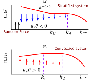
Figure 1: Schematic diagrams of energy flux $\Pi_{u}(k)$: (a) In a stably stratified flow, $\Pi_{u}(k)$ decreases with $k$ due to a negative energy supply rate $\Re\langle u_{z}(k)\theta^{*}(k)\rangle$; (b) In Rayleigh Bénard convection, $\Re\langle u_{z}(k)\theta^{*}(k)\rangle>0$, hence $\Pi_{u}(k)$ first increases for $k<k_{t}$ where $F(k)>D(k)$, then $\Pi_{u}(k)\approx\mathrm{const}$ $k_{t}<k<k_{d}$ where $F(k)\approx D(k)$; $\Pi_{u}(k)$ decreases for $k>k_{d}$ where $F(k)<D(k)$.

There is another useful flux called the entropy flux $\Pi_{\theta}$, which is defined as

$$\Pi_{\theta}(k_{0})=\sum_{k\geq k_{0}}\sum_{p<k_{0}}\delta_{\bf k,p+q}\Im([{\bf k\cdot u(q)}][{\bf\theta^{*}(k)\cdot\theta(p)}]).$$ (27)

Both, the KO and BO, phenomenologies predict a constant $\Pi_{\theta}$.

In this paper we simulate stably stratified flows and RBC, and compute the kinetic energy and entropy spectra, as well as fluxes. We also compute $F(k),D(k)$, and $d\Pi_{u}(k)/dk$, and show that our results are in good agreement with the arguments of items 2 and 3 discussed above. For stably stratified flows, the BO scaling is observed when $\mathrm{Ri}=O(1)$, but the Kolmogorov scaling $E_{u}(k)\sim k^{-5/3}$ is observed when $\mathrm{Ri}\ll 1$, or when buoyancy is negligible. RBC flows, however, exhibit the Kolmogorov scaling $E_{u}(k)\sim k^{-5/3}$ for a narrow band of wavenumbers.

III Simulation Method

We perform direct numerical simulation of stably stratified flows and RBC in a three-dimensional box by solving Eqs. (9-11) using pseudospectral code Tarang Verma et al. (2013). We employ fourth-order Runge-Kutta (RK4) method for time stepping, Courant-Freidricks-Lewey (CFL) condition for computing time step $\Delta t$, and $3/2$ rule for dealiasing.

For the stratified flows, we employ the periodic boundary conditions on all sides of a cubic box of size $(2\pi)^{3}$. To obtain a steady turbulent flow, we apply a random force to the flow in the band $2\leq k\leq 4$ using the scheme of Kimura and Herring Kimura and Herring (2012). The parameters chosen for our simulations are $\mathrm{Pr}=1.0$ (close to that of air), and Richardson numbers $\mathrm{Ri}=4\times 10^{-7},0.01$, and $0.5$. The grid resolution for $\mathrm{Ri}=0.01$ is $1024^{3}$, which is one of the largest grids for such simulations. The resolutions for $\mathrm{Ri}=4\times 10^{-7}$ and $0.5$ are $512^{3}$ grids. The parameters of our runs are listed in Table 1. All our simulations are fully resolved since $k_{\mathrm{m}ax}\eta>1$, where $k_{\mathrm{m}ax}$ is the maximum wavenumber of the run, and $\eta$ is the Kolmogorov length scale.

We simulate RBC of a fluid in a unit box with $512^{3}$ grid. The parameters of the simulation are $\mathrm{Pr}=1$ and Rayleigh number $\mathrm{Ra}=10^{7}$. For the horizontal plates, we employ free-slip boundary condition for the velocity field, and conducting boundary condition, i.e. $\theta=0$, for the temperature field. For the vertical walls, we apply periodic boundary condition for both the fields. Simulation details of RBC simulation are listed at the bottom row of the Table 1.

In the next section we will compute the the spectra and fluxes of the kinetic energy as well as that of entropy.

Table 1: Parameters of our numerical simulations for stably stratified flow (first three rows), and Rayleigh Bénard convection (the last row): Grid size, Richardson number $\mathrm{Ri}$, Rayleigh number $\mathrm{Ra}$, Reynolds number $\mathrm{Re}$, Froude number $\mathrm{Fr}$, kinetic energy dissipation rate $\epsilon_{u}$, entropy dissipation rate $\epsilon_{\theta}$, Anisotropy ratio ${E_{\perp}}/{2E_{\parallel}}$, where $E_{\perp}=(u_{x}^{2}+u_{y}^{2})/2$ and $E_{\parallel}=u_{z}^{2}/2$, $k_{max}\eta$ where $\eta$ is the Kolmogorov length, Bolgiano wavenumber $k_{B}$, and averaged $\Delta t$. We choose $\mathrm{Pr}=1$ for all the runs.

Grid	$\mathrm{Ri}$	$\mathrm{Ra}$	$\mathrm{Re}$	$\mathrm{Fr}$	$\epsilon_{u}$	$\epsilon_{\theta}$	${E_{\perp}}/{2E_{\parallel}}$	$k_{max}\eta$	$k_{B}$	$\Delta t$
$512^{3}$	$0.5$	$1\times 10^{5}$	$467$	$1.4$	$0.47$	$60.7$	$1.2$	$4.2$	$6.0$	$2.5\times 10^{-5}$
$1024^{3}$	$0.01$	$5\times 10^{3}$	$649$	$10$	$114$	$150$	$1.0$	$6.4$	$8.5$	$3.5\times 10^{-6}$
$512^{3}$	$4\times 10^{-7}$	$0.1$	$510$	$1.5\times 10^{3}$	$6.7\times 10^{8}$	$141$	$1.0$	$3.8$	$<1$	$2.6\times 10^{-6}$
$512^{3}$	$16$	$10^{7}$	$790$	NA	$8.8\times 10^{-3}$	$1.0\times 10^{-3}$	$0.41$	$2.6$	NA	$6.2\times 10^{-4}$

IV Numerical results

We compute the the spectra and fluxes of the kinetic energy as well as that of entropy using the steady-state data. We will also compute $F(k),D(k)$, and $d\Pi_{u}(k)/dk$ for the flows. These results will be discussed below.

IV.1 Stably Stratified Flow

First, we simulate stably stratified flows for $\mathrm{Pr}=1$ and $\mathrm{Ri}=0.01$ on a $1024^{3}$ grid, and compute the spectrum and flux using the steady state data. Fig. 2(a) illustrates the normalized KE spectra, $E_{u}(k)k^{11/5}$ for the BO scaling, and $E_{u}(k)k^{5/3}$ for the KO scaling. The numerical data fits with the BO scaling quite well for approximately a decade, thus confirming the phenomenology of Bolgiano and Obukhov. The normalized entropy spectra, $E_{\theta}(k)k^{7/5}$ (BO scaling) and $E_{\theta}(k)k^{5/3}$ (KO scaling), illustrated in Fig. 2(b) also show that the BO scaling is preferred for $\mathrm{Ri}=0.01$ stably stratified flow.

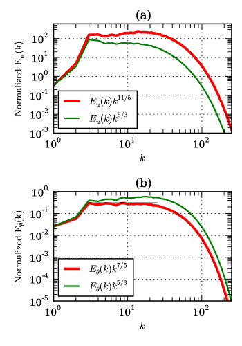
Figure 2: For stably stratified simulation with $\mathrm{Pr}=1$ and $\mathrm{Ri}=0.01$, plots of (a) normalized KE and (b) entropy spectra for Bolgiano-Obukhov (BO) and Kolmogorov-Obukhov (KO) scaling. BO scaling fits with the data better than KO scaling.

We cross check our spectrum results with the KE and entropy fluxes, which are plotted in Fig. 3. Clearly, the KE flux, $\Pi_{u}(k)$, is positive, and it decreases with $k$. However $\Pi_{u}(k)k^{4/5}$ is almost flat, thus $\Pi_{u}(k)\propto k^{-4/5}$, same as Eq. (4). We also observe that $\Pi_{\theta}$ is a constant in the inertial range [Eq. (3)]; thus flux results are consistent with the BO predictions.

We also compute the Bolgiano wavenumber $k_{B}$ Bolgiano (1959) using the numerical data, and find that $k_{B}\approx 8.5$. Our plots on spectra and fluxes show that $k_{B}\approx 8.5$ is only 3 to 4 times smaller than $k_{d}$, wavenumber where the dissipation range starts. Therefore a clear-cut crossover from $k^{-11/5}$ to $k^{-5/3}$ is not observed in our simulations. We are in the process of performing simulations on even higher resolution to probe the dual spectra ($k^{-11/5}$ and $k^{-5/3}$).

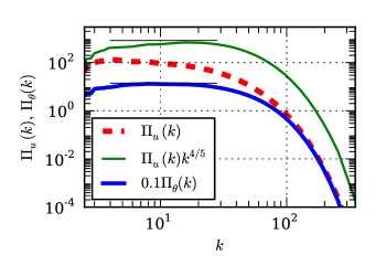
Figure 3: For stably stratified simulation with $\mathrm{Pr}=1$ and $\mathrm{Ri}=0.01$, plots of KE flux $\Pi_{u}(k)$, normalized KE flux $\Pi_{u}(k)k^{4/5}$, and entropy flux $\Pi_{\theta}(k)$.

We also compute energy supply rate by buoyancy, $F(k)=\Re\langle u_{z}(k)\theta^{*}(k)\rangle$, $D(k)$, and $d\Pi_{u}(k)/dk$ using the numerical data, and plot them in Fig. 4. The figure illustrate that $F(k)<0$, as argued in item 2 of Sec. II. The negative $F(k)$ implies that $\Pi_{u}(k)$ decreases with $k$ even without $D(k)$, which is a crucial ingredient for the BO scaling. Note that the kinetic energy flux is depleted by both $F(k)$ and $D(k)$, and they satisfy the relation of Eq. (25). Interestingly, for small $k$, $d\Pi_{u}(k)/dk\sim k^{-9/5}$ (the black line of Fig. 4), consistent with $\Pi_{u}(k)\sim k^{-4/5}$.

We also performed $512^{3}$ grid simulations for ${\rm Ri}=0.5$ and $4\times 10^{-7}$ with $\mathrm{Pr}=1$. The normalized KE spectra for these two cases are exhibited in Figs. 5(a) and  5(b) respectively. Our results show that BO scaling is valid for ${\rm Ri}=0.5$, but KO scaling (with a constant $\Pi_{u}(k)$) is valid for ${\rm Ri}=4\times 10^{-7}$, which is as expected since buoyancy is significant only for moderate and large ${\rm Ri}$’s.

We compute $F(k)$, $D(k)$, and $d\Pi_{u}(k)/dk$ for $\mathrm{Ri}=0.5$ and $4\times 10^{-7}$, and plot them in Figs. 6(a,b) respectively. In the inertial range, $F(k)<0$ for both the cases, just like $\mathrm{Ri}=0.01$. The behaviour of $F(k)$, $D(k)$, and $d\Pi_{u}(k)/dk$ for $\mathrm{Ri}=0.5$ is very similar to that of $\mathrm{Ri}=0.01$, except that $F(k)$ for $\mathrm{Ri}=0.5$ is a bit smaller than that for $\mathrm{Ri}=0.01$. For $\mathrm{Ri}=4\times 10^{-7}$, buoyancy is weak, hence $F(k)$ is much smaller than that for $\mathrm{Ri}=0.01$, which leads to an approximately constant $\Pi_{u}(k)$, and Kolmogorov’s spectrum for the kinetic energy.

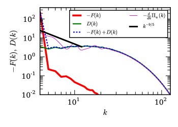
Figure 4: For stably stratified simulation with $\mathrm{Pr}=1$ and $\mathrm{Ri}=0.01$, plots of $-F(k),D(k),[-F(k)+D(k)]$, $-d\Pi_{u}(k)/dk$, and $k^{-9/5}$ line to match with $-d\Pi_{u}(k)/dk$ in the small $k$ regime.

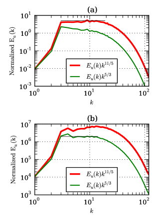
Figure 5: For stably stratified simulation with $\mathrm{Pr}=1$, and (a) $\mathrm{Ri}=0.5$ and (b) $\mathrm{Ri}=4\times 10^{-7}$, the plots of normalized KE spectra for Bolgiano-Obukhov (BO) scaling and Kolmogorov-Obukhov (KO) scaling.

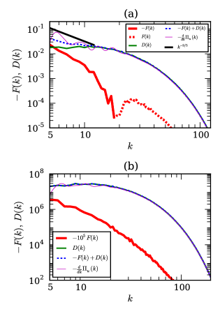
Figure 6: For stably stratified simulation with $\mathrm{Pr}=1$, and (a) $\mathrm{Ri}=0.5$ and (b) $\mathrm{Ri}=4\times 10^{-7}$, plots of $-F(k),D(k),[-F(k)+D(k)]$, $-d\Pi_{u}(k)/dk$, and $k^{-9/5}$ line to match with $-d\Pi_{u}(k)/dk$ in the small $k$ regime. In Fig. (a), the negative $F(k)$ is shown as solid red curve, and positive $F(k)$ as dashed red curve. In Fig. (b), $F(k)$ is multiplied by $10^{5}$ to fit in the same range.

Recall that we employ periodic boundary condition for the stably stratified flows in the vertical direction, thus eliminating the effects of boundary walls. In Fig. 7 we plot the plane-averaged (over $xy$ plane) mean temperature profile $\bar{T}(z)=\langle T(x,y,z)\rangle_{xy}$. Since $\bar{T}(z)$ is linear, a constant temperature gradient $d\bar{T}/dz$ (hence buoyancy) acts in the whole box. Therefore, BO scaling is expected everywhere. It is important to contrast the above profile with that for Rayleigh-Bénard convection in which most of the temperature drop takes place in the narrow thermal boundary layers at the plates Moore and Weiss (1973); Verzicco and Camussi (2003), while the bulk flow has $d\bar{T}/dz\approx 0$. Thus we expect BO scaling in the boundary layers, and KO scaling in the bulk, as reported by Calzavarini et al. Calzavarini et al. (2002).

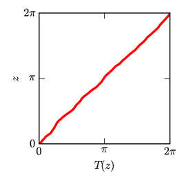
Figure 7: For stably stratified simulation with $\mathrm{Pr}=1$ and $\mathrm{Ri}=0.01$, the vertical variation of horizontally averaged mean temperature $\bar{T}(z)=\langle T(x,y,z)\rangle_{xy}$.

In the next subsection we will discuss the results of Rayleigh Bénard Convection.

IV.2 Rayleigh Bénard Convection

Borue and Orszag Borue and Orszag (1997), and S̆kandera et al. Škandera et al. (2008) simulated RBC flow under periodic boundary condition. They observed the KO scaling for both velocity and temperature fields, consistent with the arguments presented in Sec. II. A shell model approximates the turbulence in a periodic box quite well; a recent shell model of RBC flow Kumar and Verma (2014) also yields KO scaling, consistent with the numerical results of Borue and Orszag Borue and Orszag (1997), and S̆kandera et al. Škandera et al. (2008). In a typical RBC flow, however, a fluid is confined between two horizontal conducting plates that are maintained at constant temperatures, with the bottom plate hotter than the top one. Earlier, Mishra and Verma Mishra and Verma (2010) showed that zero- and small Prandtl number RBC exhibit Kolmgorov’s spectrum for the kinetic energy, but their results were inconclusive for moderate Prandtl number RBC. In this subsection, we will investigate this issue for $\mathrm{Pr}=1$.

To explore which of the two scaling (KO or BO) is applicable for RBC turbulence with plates, we perform RBC simulations for $\mathrm{Pr}=1$ and $\mathrm{Ra}=10^{7}$, and compute the spectra and fluxes of the KE as well as the entropy for the steady state data. In Fig. 8(a), we plot the normalized KE spectra for the BO and the KO scaling. The plots indicate that the KO scaling fits better than the BO scaling for a narrow band of wavenumbers (the shaded region, $15<k<40$).

We plot the KE and entropy fluxes in Fig 8(b). We also plot a zoomed view of the energy flux in Fig. 9, according to which KE flux increases till $k=22$, and then starts to decrease. In the logarithmic scale, the KE flux is an approximate constant for the wavenumbers $15<k<40$, a band where $E_{u}(k)\sim k^{-5/3}$. Thus we claim that convective turbulence exhibits Kolmogorov’s power law for a narrow band of wavenumbers. Interestingly, the energy spectrum of RBC exhibits stronger fluctuations than that of stably stratified turbulence; this feature is possibly due to the “plumes” emanating from the plates. This feature as well as a larger range of wavenumber exhibiting KO scaling may be visible in a large resolution simulation, which is planned as a future study.

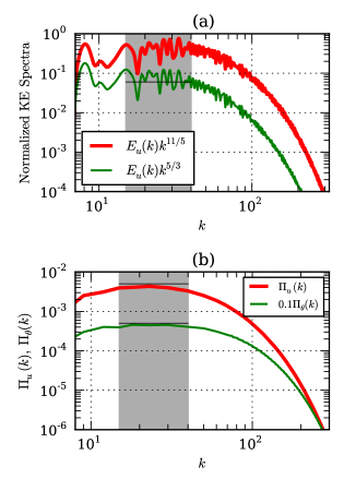
Figure 8: For RBC simulation with $\mathrm{Pr}=1$ and $\mathrm{Ra}=10^{7}$, (a) plots of normalized KE spectra for Bolgiano-Obukhov (BO) and Kolmogorov-Obukhov (KO) scaling; KO scaling fits with the data better than BO scaling;(b) KE flux $\Pi_{u}(k)$ and entropy flux $\Pi_{\theta}(k)$. The shaded region shows the inertial range.

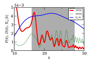
Figure 9: For RBC simulation with $\mathrm{Pr}=1$ and $\mathrm{Ra}=10^{7}$, plots of $\Pi_{u}(k)$, $F(k)$, and $D(k)$ for $10\leq k\leq 50$.

Further investigations of $F(k)$, $\Pi_{u}(k)$, and $d\Pi_{u}(k)/dk$ provide stronger evidence for the KO scaling in RBC. We plot these quantities in Figs. 9 and 10, according to which $F(k)>0$, consistent with the discussion of Sec. II and Fig. 1(b). In addition, for the wavenumber band $7<k<22$, $F(k)>D(k)$, hence, according to Eq. (25), $d\Pi_{u}(k)/dk>0$. Therefore, $\Pi_{u}(k)$ increases in this band of wavenumbers, as illustrated in Fig. 9. But for $k>22$, we find that $D(k)>F(k)$ leading to $d\Pi_{u}(k)/dk<0$, therefore, $\Pi_{u}(k)$ decreases with $k$ for this range of $k$. However, for a narrow band of wavenumbers $15<k<40$, $F(k)\approx D(k)$, hence $d\Pi_{u}(k)/dk\approx 0$ or $\Pi_{u}(k)\approx\mathrm{const}$. The constancy of $\Pi_{u}(k)$ yields $E_{u}(k)\sim k^{-5/3}$, consistent with the energy spectrum plots of Fig. 8. Note that many simulations, including Mishra and Verma Mishra and Verma (2010), reported that $\Pi_{u}(k)\sim k^{-4/5}$ for moderate $\mathrm{Pr}$, but the decrease of $\Pi_{u}(k)$ in their work is essentially due to $D(k)$, not due to buoyancy.

Thus, the flux and energy supply due to buoyancy reveal that convective turbulence follows KO scaling, at least for a narrow range of wavenumbers. The BO scaling is ruled out for RBC since $F(k)>0$.

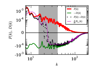
Figure 10: For RBC simulation with $\mathrm{Pr}=1$ and $\mathrm{Ra}=10^{7}$, plots of $F(k)$, $-D(k)$, $F(k)-D(k)$, and $d\Pi_{u}(k)/dk$. $d\Pi_{u}(k)/dk>0$ for $k<22$, but $<0$ for $k>22$.

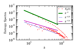
Figure 11: For RBC simulation with $\mathrm{Pr}=1$ and $\mathrm{Ra}=10^{7}$, plots of the entropy spectrum, that exhibits dual branch. The upper branch matches with $k^{-2}$ quite well, while the lower part is fluctuating.

The entropy $(\theta^{2}/2)$ is a useful quantity in RBC. The entropy flux, illustrated in Fig. 8(b), is constant for the narrow inertial range $(15<k<40)$. In Fig. 11, we plot the entropy spectrum that exhibits dual branch, with the upper branch scaling as $k^{-2}$. Mishra and Verma Mishra and Verma (2010), and Pandey et al. Pandey et al. (2014) showed the dominant temperature modes $\theta(0,0,2n)$, which are approximately $-1/(2n\pi)$ where $n$ is an integer, constitute the $k^{-2}$ branch of the entropy spectrum. They showed that $\theta(0,0,2n)$ modes are responsible for the steep temperature variations in the thermal boundary layers of the plates. Interestingly, the temperature modes in both the branches of the entropy spectrum participate to yield a constant entropy flux in the inertial range.

V Conclusions

We performed large resolution simulations of stably stratified flows and Rayleigh Bénard convection, and studied the spectra and fluxes of the kinetic energy and entropy. We also compute the energy supply rate due to buoyancy that provide important clues on the underlying turbulence phenomena.

For stably stratified turbulence, we show that the kinetic energy spectrum $E_{u}(k)\sim k^{-11/5}$, the energy flux $\Pi_{u}(k)\sim k^{-4/5}$, the entropy spectrum $E_{\theta}(k)\sim k^{-7/5}$, and the entropy flux $\Pi_{\theta}(k)\sim\mathrm{const}$, in agreement with the prediction of Bolgiano and Obukhov, referred to as BO scaling. We also compute the energy supply rate by buoyancy, and find that to be negative, signalling the buoyancy-induced conversion of kinetic energy to potential energy.

For the Rayleigh Bénard convection, the energy supply rate due to buoyancy, $F(k)$, is positive. Hence the kinetic energy flux $\Pi_{u}(k)$ first increases with $k$, and then flattens for a narrow band of wavenumbers, and finally decreases with $k$; the three regimes correspond to $F(k)>D(k)$, $F(k)\approx D(k)$, and $F(k)<D(k)$, respectively, where $D(k)$ is the dissipation spectrum. We observe Kolmogorov’s spectrum ($k^{-5/3}$) for wavenumbers where $F(k)\approx D(k)$ or $\Pi_{u}(k)\approx\mathrm{const}$. Thus, a detailed investigation of the kinetic energy flux, the energy supply due to buoyancy, and the dissipation spectrum provide valuable inputs that rule out BO scaling for RBC, contrary to the predictions of Procaccia and Zeitak Procaccia and Zeitak (1989), L’vov L’vov (1991), L’vov and Falkovich L’vov and Falkovich (1992), and Rubinstein Rubinstein (1994). The entropy flux for RBC is constant in the inertial range, but the entropy spectrum exhibit dual branch, whose origin is related to the thermal boundary layer.

In summary, stably stratified flows exhibit BO scaling in buoyancy dominated regime. Turbulent convection however exhibits Kolmogorov’s spectrum, rather than BO spectrum. A recent shell model of buoyancy-driven flows Kumar and Verma (2014) shows similar results. More work, specially very large resolution simulations, are required to explore dual spectra predicted by Bolgiano and Obukhov.

Appendix A Scaling of the equations

Many researchers, e.g.  Lindborg (2006); Brethouwer et al. (2007), have nondimensionalized Eqs. (5-7) as the following. They choose the characteristic horizontal velocity $U_{\perp}$ as the horizontal velocity scale, the horizontal length $l_{\perp}$ and the vertical height $l_{\parallel}$ as the horizontal and vertical length scales respectively, $l_{\perp}/U_{\perp}$ as the time scale, $U_{\perp}\mathrm{Fr}_{\perp}^{2}/\alpha$ as the vertical velocity scale where $\alpha=l_{\parallel}/l_{\perp}$ is the aspect ratio, and $U_{\perp}^{2}\rho_{0}/(gl_{\parallel})$ as the density scale. In terms of non-dimensional variables, the equations are

$$D_{1}\bf u_{\perp} = -{\nabla_{\perp}\sigma}+\frac{1}{\mathrm{Re}}D_{2}\bf u_{\perp},$$ (28)

$$\mathrm{Fr}_{\perp}^{2}D_{1}\bf u_{\parallel} = -\frac{d\rho}{dz}-\rho+\frac{\mathrm{Fr}_{\perp}^{2}}{\mathrm{Re}}D_{2}\bf u_{\parallel},$$ (29)

$$D_{1}\rho = u_{z}+\frac{1}{\mathrm{RePr}}D_{2}\rho,$$ (30)

$$\nabla_{\perp}\cdot\bf u_{\perp} = -\frac{\mathrm{Fr}_{\perp}^{2}}{\alpha^{2}}\frac{\partial{\bf u_{\parallel}}}{\partial z},$$ (31)

where

$$D_{1} = \frac{\partial}{\partial t}+({\bf u_{\perp}\cdot\nabla_{\perp}})+\frac{\mathrm{Fr}_{\perp}^{2}}{\alpha^{2}}{u_{z}}\frac{\partial}{\partial z}$$ (32)

$$D_{2} = \frac{1}{\alpha^{2}}\frac{\partial^{2}}{\partial z^{2}}+\nabla_{\perp}^{2}.$$ (33)

Here $\mathrm{Fr}_{\perp}=U_{\perp}/(l_{\perp}\mathrm{N})$ is the horizontal Froude number, and $\mathrm{N}=\sqrt{(g/\rho_{0})|d\bar{\rho}/dz}|$ is the Brunt-Väisälä frequency.

References

- Siggia (1994) E. D. Siggia, Ann. Rev. Fluid Mech. 26, 137 (1994).
- Lohse and Xia (2010) D. Lohse and K. Q. Xia, Ann. Rev. Fluid Mech. 42, 335 (2010).
- Bolgiano (1959) R. Bolgiano, J. Geophys. Res. 64, 2226 (1959).
- Obukhov (1959) A. N. Obukhov, Dokl. Akad. Nauk SSSR 125, 1246 (1959).
- Kimura and Herring (1996) Y. Kimura and J. R. Herring, J. Fluid Mech. 328, 253 (1996).
- Kimura and Herring (2012) Y. Kimura and J. R. Herring, J. Fluid Mech. 698, 19 (2012).
- Lindborg (2005) E. Lindborg, Geo. Res. Lett. 32, 207 (2005).
- Lindborg (2006) E. Lindborg, J. Fluid Mech. 550, 207 (2006).
- Brethouwer et al. (2007) G. Brethouwer, P. Billant, E. Lindborg, and J.-M. Chomaz, J. Fluid Mech. 585, 343 (2007).
- Vallgren et al. (2011) A. Vallgren, E. Deusebio, and E. Lindborg, Phys. Rev. Lett. 107, 268501 (2011).
- Bartello and Tobias (2013) P. Bartello and S. M. Tobias, J. Fluid Mech. 725, 1 (2013).
- Procaccia and Zeitak (1989) I. Procaccia and R. Zeitak, Phys. Rev. Lett. 62, 2128 (1989).
- L’vov (1991) V. S. L’vov, Phys. Rev. Lett. 67, 687 (1991).
- L’vov and Falkovich (1992) V. S. L’vov and G. E. Falkovich, Physica D 57, 85 (1992).
- Rubinstein (1994) R. Rubinstein, NASA Technical Memorandum 1066602 (1994).
- Borue and Orszag (1997) V. Borue and S. A. Orszag, J. Sci. Comput. 12, 305 (1997).
- Škandera et al. (2008) D. Škandera, A. Busse, and W. C. Müller, High Performance Computing in Science and Engineering, Transactions of the Third Joint HLRB and KONWIHR Status and Result Workshop (Springer, Berlin), Part IV, p. 387 (2008).
- Mishra and Verma (2010) P. K. Mishra and M. K. Verma, Phys. Rev. E 81, 056316 (2010).
- Verzicco and Camussi (2003) R. Verzicco and R. Camussi, J. Fluid Mech. 477, 19 (2003).
- Camussi and Verzicco (2004) R. Camussi and R. Verzicco, Eur. J. of Mech. /B Fluids 23, 427 (2004).
- Calzavarini et al. (2002) E. Calzavarini, F. Toschi, and R. Tripiccione, Phys. Rev. E 66, 016304 (2002).
- Wu et al. (1990) X. Z. Wu, L. Kadanoff, A. Libchaber, and M. Sano, Phys. Rev. Lett. 64, 2140 (1990).
- Chillá et al. (1993) F. Chillá, S. Ciliberto, C. Innocenti, and E. Pampaloni, Nuovo Cimento D 15, 1229 (1993).
- Cioni et al. (1995) S. Cioni, S. Ciliberto, and J. Sommeria, Europhys Lett 32, 413 (1995).
- Niemela et al. (2000) J. J. Niemela, L. Skrbek, K. R. Sreenivasan, and R. J. Donnelly, Nature 404, 837 (2000).
- Zhou and Xia (2001) S. Q. Zhou and K. Q. Xia, Phys. Rev. Lett. 87, 064501 (2001).
- Shang and Xia (2001) X. D. Shang and K. Q. Xia, Phys. Rev. E 64, 065301 (2001).
- Mashiko et al. (2004) T. Mashiko, Y. Tsuji, T. Mizuno, and M. Sano, Phys. Rev. E 69, 036306 (2004).
- Zhang et al. (2005) J. Zhang, X. L. Wu, and K. Q. Xia, Phys. Rev. Lett. 94, 174503 (2005).
- Sun et al. (2006) C. Sun, Q. Zhou, and K. Q. Xia, Phys. Rev. Lett. 97, 144504 (2006).
- Lorenz (1954) E. N. Lorenz, Tellus 7, 157 (1954).
- Davidson (2013) P. A. Davidson, Turbulence in Rotating Stratified and Electrically Conducting Fluids (Cambridge University Press, Cambridge, 2013).
- Lesieur (2008) M. Lesieur, Turbulence in Fluids - Stochastic and Numerical Modelling (Kluwer Academic Publishers, Dordrecht, 2008).
- Verma (2012) M. K. Verma, Europhys Lett 98, 14003 (2012).
- Verma (2004) M. K. Verma, Phys. Rep. 401, 229 (2004).
- Verma et al. (2013) M. K. Verma, A. G. Chatterjee, K. S. Reddy, R. K. Yadav, S. Paul, M. Chandra, and R. Samtaney, Pramana 81, 617 (2013).
- Moore and Weiss (1973) D. Moore and N. Weiss, J. Fluid Mech. 58, 289 (1973).
- Kumar and Verma (2014) A. Kumar and M. K. Verma, Arxiv preprint arXiv:1406.5360 (2014).
- Pandey et al. (2014) A. Pandey, M. K. Verma, and P. K. Mishra, Phys. Rev. E 89, 023006 (2014).