Mass-loss rates of Very Massive Stars

Abstract

We discuss the basic physics of hot-star winds and we provide mass-loss rates for (very) massive stars. Whilst the emphasis is on theoretical concepts and line-force modelling, we also discuss the current state of observations and empirical modelling, and address the issue of wind clumping.

1 Introduction

Mass loss via stellar winds already plays a well-documented role in the evolution of canonical 20-60 $M_{\odot}$ O stars, because of the removal of mass from the outer layers, as well as the removal of angular momentum. However, nowhere is mass loss more dominant than for the most massive stars. As very massive stars (VMS) evolve structurally close to chemically homogeneously, the detailed mixing processes due to rotation and magnetic fields are less relevant than for canonical massive stars. Instead, VMS evolution is determined by mass loss (Yungelson et al. 2008; Yusof et al. 2013; Köhler et al. 2014). However, there is uncertainty regarding the quantitative mass-loss rates, partly because of uncertain physics in close proximity to the Eddington ($\Gamma$) limit, and partly because O-star winds are inhomogeneous and clumpy, implying that empirical mass-loss rates are overestimated if one does not properly take clumping effects into account in the analysis.

In this mass-loss chapter, we start off in Sect. 2 with the mass-loss theory of canonical 20-60 $M_{\odot}$ O-star winds, which are optically thin, and where the traditional CAK theory due to Castor, Abbott & Klein (1975) is applicable. For VMS, the role of radiation pressure over gas pressure is even more important than for normal massive stars, and as VMS are in closer proximity to the $\Gamma$ limit, at some point their winds are expected to become optically thick.

In Sect. 3, we discuss the optically thick wind theory for classical Wolf-Rayet (WR) stars with very strong emission lines and dense winds. Once we have reached a basic understanding of both optically thin and optically thick winds, we discuss the transition from O to WR star winds in the context of VMS in Sect. 4. VMS are associated with WR stars of the WNh subtype. WNh implies the presence of both hydrogen (H) and nitrogen (N) at the surface. The latter is thought to have originated in the CNO-cycle, and reaching the surface through mass loss and (rotational) mixing. WNh stars are thought to be core H-burning (see Martins’ Chapter 2) and can thus be considered “O-stars on steroids”. The reason they have a WR type spectrum is due to their strong winds, because of the proximity to the Eddington limit.

Another group of objects that may be relevant for VMS evolution are the Luminous Blue Variables (LBVs). Already in quiescence these objects reside in dangerous proximity to the Eddington limit, where they are subjected to outbursts and mass ejections. A discussion of both “quiet” and super-Eddington winds relevant to both the characteristic “moderate” S Dor variations and the “giant” outbursts, such as displayed by Eta Car in 1840, as well as the theory of super-Eddington winds are thus discussed in Sect. 6.

After this theoretical overview of homogeneous stellar winds, we consider clumped winds. To this purpose, we first discuss the diagnostics of smooth winds (Sect. 7) before turning to clumped winds in Sect. 8. We finish Sect. 8 with potential theories that may cause wind clumping, as well as some possibilities to quantify the number of clumps, before we summarise in Sect. 9.

For the 2D effects of rotation on stellar winds, we refer to the review by Puls et al. (2008) and for more recent calculations to Müller & Vink (2014), which also includes a discussion of the diagnostics of axi-symmetric outflows.

2 O stars with optically thin winds

As each photon carries a momentum, $P=h\nu/c$, it was thought as early as the 1920s (e.g. Milne 1926) that radiative acceleration on spectral lines might selectively “eject” metal ions (such as iron, Fe) from stellar photospheres. However, it was not until the arrival of ultraviolet (UV) observations in the late 1960s that the theory of radiative line driving became the established theory describing the stationary outflows from massive OB stars. Lucy & Solomon (1970) and CAK showed that in case the momentum imparted on metal ions was shared through Coulomb interactions with the more abundant H and helium (He) species in the atmospheric plasma, this would result in a substantial rate of mass loss $\dot{M}$, affecting the evolution of massive stars significantly (Conti 1976; Langer et al. 1994; Meynet & Maeder 2003; Eldrige & Vink 2006; Limongi & Chieffi 2006; Belkus et al. 2007; Brott et al. 2011; Hirschi’s Chapter 6; and Woosley & Heger’s Chapter 7).

2.1 Stellar wind equations

The basic idea of momentum transfer by line-scattering is that absorbed photons originate from a preferred direction, whereas the subsequent re-emission is averaged to be (more or less) isotropic. This change in direction angle $\theta$ leads to a radial transfer of momentum, $\Delta P=h/c(\nu_{\rm in}\cos\theta_{\rm in}-\nu_{\rm out}\cos\theta_{\rm out})$ – comprising the key to the momentum transfer with its associated line acceleration $g_{\rm rad}^{\rm line}$. The mass-loss rate through a spherical shell with radius $r$ that surrounds the star is conserved, as may be noted from the equation of mass continuity

$$\dot{M}=4\,\pi\,r^{2}\,\rho\,(r)\,v\,(r).$$ (1)

The equation of motion is given by:

$$v\frac{{\rm d}v}{{\rm d}r}~{}=~{}-\frac{GM}{r^{2}}~{}-~{}\frac{1}{\rho}\frac{{\rm d}p}{{\rm d}r}~{}+~{}g_{\rm rad},$$ (2)

with inwards directed gravitational acceleration $g_{\rm grav}=GM/r^{2}$ and an outwards directed gas pressure ($p$) term and total (continuum and line) radiative acceleration ($g_{\rm rad}$). The wind initiation condition is that the total radiative acceleration, $g_{\rm rad}$ = $g^{\rm line}_{\rm rad}$ $+$ $g^{\rm cont}_{\rm rad}$ exceeds gravity beyond a certain point. With the equation of state, $p=a^{2}\,\rho$, where $a$ is the isothermal sound speed, the equation becomes:

$$\bigl{(}1-\frac{a^{2}}{v^{2}}\bigr{)}~{}v\frac{{\rm d}v}{{\rm d}r}~{}=~{}\frac{2a^{2}}{r}~{}-~{}\frac{{\rm d}a^{2}}{{\rm d}r}~{}-~{}\frac{GM}{r^{2}}~{}~{}+~{}g_{\rm rad}.$$ (3)

The prime challenge lies in accurately computing $g_{\rm rad}$. For free electrons this concerns the Thomson opacity, $\sigma_{\rm e}=s_{\rm e}\rho$ ($s_{\rm e}$ proportional to cross section) and the flux:

$$g^{\rm Th}_{\rm rad}~{}=~{}\frac{1}{c\rho}\frac{\sigma_{\rm e}L}{4\pi r^{2}}~{}=~{}g_{\rm grav}\,\Gamma,$$ (4)

with the Eddington parameter $\Gamma$ representing the radiative acceleration over gravity, given by:

$$\Gamma=\frac{\kappa L}{4\pi cGM}.$$ (5)

Spectral lines provide the dominant contribution to the overall radiative acceleration. The reason is that line scattering is intrinsically much stronger than electron scattering because of the resonant nature of bound-bound transitions (Gayley 1995), and although photons and matter are only allowed to interact at specific frequencies, they can be made to resonate over a wide range of stellar wind radii via the Doppler effect (see Owocki’s Chapter 5).

For a single line at frequency $\nu$, with line optical depth $\tau$, the line acceleration can be approximated by local quantities (Sobolev 1960). This approximation is valid as long as opacity, source function, and the velocity gradient ($dv/dr$) do not change significantly over a velocity range $\Delta v=\mbox{$v_{\rm th}$}$, corresponding to a spatial region $\Delta r\approx\mbox{$v_{\rm th}$}/(\mbox{${\rm d}v/{\rm d}r$})$, i.e. the Sobolev length. In the Sobolev approximation, the line acceleration becomes:

$$g^{\rm line}_{\rm rad,i}~{}=~{}\frac{L_{\nu}\nu}{4\pi r^{2}c^{2}}~{}(\frac{{\rm d}v}{{\rm d}r})~{}\frac{1}{\rho}~{}(1~{}-~{}e^{-\tau}),$$ (6)

with $L_{\nu}$ the luminosity at the line frequency, and with

$$\tau=\bar{\kappa}\lambda/(\mbox{${\rm d}v/{\rm d}r$}),$$ (7)

where $\bar{\kappa}$ represents the frequency integrated line-opacity and $\lambda$ is the wavelength of the transition. For optically thin lines ($\tau<1$) the line acceleration has the same $1/r^{2}$ dependence as electron scattering (Eq. 4), whereas for optically thick lines ($\tau>1$) it depends on the velocity gradient (${\rm d}v/{\rm d}r$), which is the root cause for the peculiar nature of line driving.

2.2 CAK solution

The next step is to sum the line acceleration over all lines. In the CAK theory this is achieved through the line-strength distribution function that describes the statistical dependence of the number of lines on frequency position and line-strength (e.g. Puls et al. 2000). Combining the radiative line acceleration (Eq. 6) with the distribution of lines, the total line acceleration can be calculated by integration. It can be expressed in terms of the Thomson acceleration (Eq. 4) multiplied by the famous force-multiplier $M(t)$,

$$M(t)~{}=~{}\frac{g^{\rm line}_{\rm rad}}{g^{\rm TH}_{\rm rad}}~{}=~{}k~{}t^{-\alpha}\propto\bigl{(}\frac{\mbox{${\rm d}v/{\rm d}r$}}{\rho}\bigr{)}^{\alpha},$$ (8)

where $k$ and $\alpha$ are the so-called force multiplier parameters.

For the complete distribution of lines, the radiative acceleration depends on (${\rm d}v/{\rm d}r$) through the power of $\alpha$. CAK postulated that this term has a similar meaning as the velocity gradient entering the inertial term on the left hand side of Eq. 3. Assuming this is the case, the equation of motion becomes non-linear, and can be solved through a critical point that sets the mass-loss rate $\dot{M}$:

$$\dot{M}\propto(kL)^{1/\alpha}~{}(M(1-\Gamma))^{1-1/\alpha}.$$ (9)

And with velocity:

$$v(r)=\mbox{$v_{\infty}$}(1~{}-~{}R/r)^{\beta}$$ (10)

$$\mbox{$v_{\infty}$}=\mbox{$C_{\infty}$}\bigl{(}\frac{2GM(1-\Gamma)}{\mbox{$R_{\ast}$}}\bigr{)}^{\mbox{$\frac{1}{2}$}}=\mbox{$C_{\infty}$}v_{\rm esc},$$ (11)

where $C_{\infty}$ $\approx$ 2.6 for O stars, and $v_{\rm esc}$ is the photospheric escape velocity corrected for Thomson electron acceleration. $\beta$ is exactly 0.5 for a point source, and in the range $\beta\,\approx\,0.8-1$ for more realistic (finite sized) objects (Pauldrach et al. 1986; Müller & Vink 2008). For O stars, $\alpha\simeq 0.6$ and $k$ is of the order of 0.1.

Using these relations, one can construct the modified wind momentum rate, $\mbox{$D_{\rm mom}$}\,=\,\mbox{$\dot{M}$}\,\mbox{$v_{\infty}$}\,(\mbox{$R_{\ast}$}/\mbox{$R_{\odot}$})^{1/2}$. Given that $v_{\infty}$ scales with the escape velocity (Eq. 11), $D_{\rm mom}$ scales with luminosity and effective line number only, and as long as $\alpha$ $\simeq$ $2/3$, the effective mass $M(1-\Gamma)$ conveniently cancels from the product $\dot{M}$ $v_{\infty}$, resulting in:

$$\log\mbox{$D_{\rm mom}$}~{}\approx~{}x~{}\mbox{$\log(L/L_{\odot})$}+D,$$ (12)

(with slope $x$ and offset $D$, depending on the flux-weighted number of driving lines), the “wind momentum luminosity relationship (WLR)” (Kudritzki et al. 1995; Puls et al. 1996; Vink et al 2000). The relationship played an instrumental role in determining the empirical mass-loss metallicity ($Z$) dependence for O stars in the Local Group (Mokiem et al. 2007), and observed and predicted WLRs can be compared to test the validity of the theory, and to highlight potential shortcomings, e.g. concerning wind clumping. One should also realise that $\dot{M}$ is not only a function of $L$ but also parameters like $T_{\rm eff}$. One should properly account for this multivariate behaviour of $\dot{M}$ when one attempts to compare observations to theory, and when one wishes to properly assess the effects of stellar wind mass loss in stellar evolution modelling.

We note that all CAK-type relations are only valid for spatially constant force multiplier parameters, $k$ and $\alpha$, which is not the case in more realistic models (Vink 2000; Kudritzki 2002; Muijres et al. 2012a). Other assumptions involve the adoption of a core-halo structure, and the neglect of multi-line effects.

2.3 Predictions using a Monte Carlo radiative transfer approach

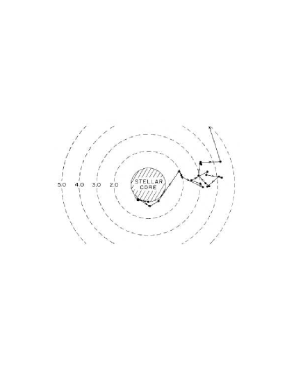
Figure 1: Cartoon explaining the Monte Carlo method: photon path histories are tracked on their outwards journey. From Abbott & Lucy (1985).

An alternative approach to CAK involves the Monte Carlo method developed by Abbott & Lucy (1985). Here photon-scattering histories are tracked on their journey outwards. At each interaction, momentum and energy are transferred from the photons to the ions (see Fig. 1). One of the major advantages of the Monte Carlo method is that it easily allows for multi-line scattering, which becomes important in denser winds. Prior to the year 2000, theoretical mass-loss rates fell short of the observed rates for dense O star and WR winds, whilst for weak winds the oft-used single line approach overestimated mass-loss rates. The crucial point is that multiply scattered photons add radially outward momentum to the wind, and the momentum may exceed the single-scattering limit, i.e., $\eta=\mbox{$\dot{M}$}\mbox{$v_{\infty}$}/(L/c)$ can become larger than unity. The overall $\dot{M}$ can be obtained from global energy conservation:

$$\frac{1}{2}\mbox{$\dot{M}$}(\mbox{$v_{\infty}$}^{2}+v_{\rm esc}^{2})=\Delta L,$$ (13)

where $\Delta L$ is the total energy transferred per second from the radiation to the outflowing particles.

Vink et al. (2000, 2001) used the Monte Carlo method to derive a mass-loss recipe, where for objects hotter than the so-called bi-stability jump at $\simeq 25~{}000$ K, the rates roughly scale as:

$$\mbox{$\dot{M}$}~{}\propto~{}L^{2.2}~{}M^{-1.3}~{}\mbox{$T_{\rm eff}$}~{}(\mbox{$v_{\infty}$/$v_{\rm esc}$})^{-1.3}.$$ (14)

The success of the Monte Carlo method is highlighted through the comparison of observed and predicted mass-loss rates in Vink (2006). Figures 1 and 4 of that review display the level of agreement between modified CAK models and observations on the one hand, and the Vink et al. (2000) predictions on the other hand. Despite remaining uncertainties due to an unknown amount of wind clumping, by properly including multiple scatterings, the results were shown to be equally successful for relatively weak (with $\dot{M}$ $\sim$ $10^{-7}$ $M_{\odot}{\rm yr}^{-1}$) as dense O-star winds (with $\dot{M}$ $\sim$ $10^{-5}$ $M_{\odot}{\rm yr}^{-1}$). The predictions can also be expressed via the WLR. For O-stars hotter than 27 500 K, the relation is shown in Fig. 2 and given by Eq. (12) with a slope $x$ $=$ 1.83.

Figure 2: Predicted WLR for O stars hotter than 27 kK for a range of $(L,M)$-combinations in the upper HR diagram. From Vink et al. (2000).

Traditionally, the prime drawback of the Monte Carlo approach was the usage of a pre-determined $v_{\infty}$ (guided by accurate empirical values) but this assumption can be dropped, as discussed in the following.

2.4 Line acceleration formalism $g(r)$ for Monte Carlo use

In solving the equation of motion self-consistently without relying on any free parameters, Müller & Vink (2008) determined the velocity field through the use of a parameterised description of the line acceleration that only depends on radius (rather than explicitly on the velocity gradient dv/dr as in CAK theory.) The line acceleration was obtained from Monte Carlo radiative transfer calculations. As this acceleration is determined in a statistical way, it shows scatter, and given the delicate nature of the equation of motion it should be represented by an appropriate analytic fit function. Müller & Vink (2008) motivated:

$$\mathit{g}_{\rm rad}^{\rm line}=\left\{\begin{array}[]{rl}0&\hskip 17.07164pt\textrm{if }\hskip 5.69054ptr<r_{\circ}\\ \mathit{g}_{\circ}\,(1-r_{\circ}/r)^{\gamma}/r^{2}&\hskip 17.07164pt\textrm{if }\hskip 5.69054ptr\geq r_{\circ},\\ \end{array}\right.$$ (15)

where $\mathit{g}_{\circ}$, $r_{\circ}$, and $\gamma$ are fit parameters to the Monte Carlo line acceleration. Müller & Vink (2008) derived an analytic solution of the velocity law in the outer wind, which was compared to the standard CAK $\beta$-law and subsequently used to derive $v_{\infty}$ and the most representative $\beta$ value.

Equation 3 is a critical point equation, where the left- and right-hand side vanish at the point $v(r_{s})=a_{\circ}$, i.e. where $r_{s}$ is the sonic-point radius. Müller & Vink (2008) showed that for the isothermal case and a line acceleration as described in Eq. 15, analytic expressions for all types of solutions of Eq. 3 can be constructed by means of the Lambert W function. A useful approximate wind solution for the velocity law can be constructed if the gas pressure related terms $2a^{2}/r$ and $a/v$ are neglected. After some manipulation one obtains the approximate velocity law:

$$v(r)=\sqrt{\frac{R_{*}v_{\rm esc}^{2}}{r}+\frac{2}{r_{\circ}}\frac{\mathit{g}_{\circ}}{\left(1+\gamma\right)}\left(1-\frac{r_{\circ}}{r}\right)^{\gamma+1}+C},$$ (16)

where $C$ is an integration constant. From this equation the terminal wind velocity can be derived if the integration constant $C$ can be determined, which can be done by assuming that at radius $r_{\circ}$ the velocity approaches zero, resulting in:

$$C=-\frac{R_{*}v_{\rm esc}^{2}}{r_{\circ}}.$$ (17)

In the limit $r\rightarrow\infty$:

$$\mbox{$v_{\infty}$}=\sqrt{\frac{2}{r_{\circ}}{\frac{\mathit{g}_{\circ}}{(1+\gamma)}-\frac{R_{*}v_{\rm esc}^{2}}{2}}}.$$ (18)

The terminal velocity $v_{\infty}$ can also be determined from the equation of motion. At the critical point, the left-hand and right-hand side of Eq. 3 both equal zero. Introducing $v_{\infty}$ in relation to $\mathit{g}_{\circ}$ as expressed in Eq. 18, one obtains

$$v_{\infty,{\rm new}}=\sqrt{\frac{2}{r_{\circ}}\left[\left(\frac{r_{s}}{r_{s}-r_{\circ}}\right)^{\gamma}\frac{r_{s}}{(1+\gamma)}\left(\frac{v_{\rm esc}}{2}-2r_{s}\right)-v_{\rm esc}^{2}\right]}.$$ (19)

A direct comparison to the $\beta$-law can be made for the supersonic regime of the wind, resulting in

$$\beta=\frac{1+\gamma}{2}.$$ (20)

The procedure to obtain the best-$\beta$ solution is that in each iteration step of the Monte Carlo simulation the values of $\mathit{g}_{\circ}$, $r_{\circ}$, and $\gamma$ are determined by fitting the output line acceleration. Using these values and the radius of the sonic point, Eqs. 18, 19 and 20 are used to determine $v_{\infty}$ and $\beta$. $v_{\infty}$ derived from Eq. 19, the predicted mass-loss rate, and the expression derived for $\beta$ serve as input for the next model, with iterations continuing until convergence is achieved.

Muijres et al. (2012a) tested the Müller & Vink (2008) wind solutions through explicit numerical integrations of the fluid equation, also accounting for a temperature stratification, obtaining results that were in excellent agreement with the Müller & Vink solutions. These solutions were extended to 2D in Müller & Vink (2014).

3 Wolf-Rayet stars with optically thick winds

Figure 3: Comparison of mass-loss rates from WR and Galactic O supergiants (from Puls et al. 2008). Solid and dotted lines represent mean relations for H-poor WN (solid) and WC stars (dotted) from Nugis & Lamers (2000). The dashed line corresponds to Galactic O supergiants – taken from the Mokiem et al. (2007) WLR.

3.1 Wolf-Rayet (WR) stars

WR stars can be divided into nitrogen-rich WN stars and carbon/oxygen rich WC/WO stars. The principal difference between the two subtypes is believed to be that the N-enrichment in WN stars is a by-product of H-burning, whereas the C/O in WC/WO stars is due to the arrival of He-burning products at the surface, showing strong emission lines of He, C and O.

The WR classification is purely spectroscopic, signalling the presence of strong and broad emission lines. Such spectra can originate in evolved stars, or alternatively from objects that formed with high initial masses and luminosities, the VMS. This latter group of WR stars may thus include objects still in their core H-burning phase of evolution: WNh stars.

Stellar radii determined from sophisticated non-LTE models are a factor of several ($\sim$3) larger than those predicted for the He-main sequence by stellar evolution modelling. In other words, there is a radius problem, and a potential solution might involve the inflation of a clumped outer envelope (Gräfener et al. 2012; See Chapter 5 for more details).

3.2 WR wind theory

WR stars have strong winds with large mass-loss rates, typically a factor of 10 larger than O-star winds with the same luminosity (see Fig. 3), and they are not easily explained by the optically thin line-driven wind theory by CAK. The observed wind efficiency $\eta$ values are typically in the range of 1-5, i.e. well above the single-scattering limit. So, if WR-type winds are driven by radiation, photons must be scattered more than once. As the ionisation equilibrium decreases outwards, photons can interact with lines from a variety of different ions on their way out, whilst gaps between lines become “filled in” (see Lucy & Abbott 1993; Schaerer & Schmutz 1994; Springmann 1994; Gayley et al. 1995).

The initiation of the mass loss relies on the condition that the winds are already optically thick at the sonic point and that the photospheric line acceleration due to the high opacity “iron peak” may overcome gravity, thus driving a wind (Nugis & Lamers 2002).

The crucial point in such a critical-point analysis for optically thick winds is that due to their large mass-loss rates, the atmospheres become so extended and the sonic point of the wind is already reached at large flux-mean optical depth $\tau_{s}$, which implies that the radiation can be treated in the diffusion approximation. The equation for the radiative acceleration can then be approximated to:

$$g_{\rm rad}=\frac{1}{c}\int\kappa_{\nu}F_{\nu}{\rm d}\nu=\kappa_{\rm Ross}\frac{L_{\star}}{4\pi r^{2}c},$$ (21)

where $\kappa_{\rm Ross}$ is the Rosseland mean opacity which can be taken from for instance the OPAL opacity tables (Iglesias & Rogers 1996). As $g_{\rm rad}$ does not depend on ($\frac{{\rm d}v}{{\rm d}r}$) Eq. (3) has a critical point at the sonic point $r_{\rm s}$ where $v=a$.

A finite value of ($\frac{{\rm d}v}{{\rm d}r}$) can only be obtained if the right hand side of Eq. (3) is zero at this point.

$$0=-\frac{GM}{r_{\rm s}^{2}}+\frac{2a^{2}}{r_{\rm s}}-\frac{{\rm d}a^{2}}{{\rm d}r_{\rm s}}+g_{\rm rad}.$$ (22)

For reasonable wind parameters the second and third term on the right-hand side of Eq. (22) become zero such that

$$\frac{GM}{r_{\rm s}^{2}}\simeq g_{\rm rad}(r_{\rm s})\equiv\kappa_{\rm crit}\frac{L_{\star}}{4\pi r_{\rm s}^{2}c}.$$ (23)

The Eddington limit with respect to the Rosseland mean opacity is thus crossed at the sonic point, and $\kappa_{\rm crit}$ for the Rosseland mean opacity can be computed for stellar parameters in terms of the ($L/M$) ratio.

In Fig. 4 the solution of Eq. (23) is plotted. This figure shows the relation between density and temperature with $\kappa_{\rm Ross}(\rho,T)=\kappa_{\rm crit}$, for a typical WC star. Below the sonic point, $r_{\rm s}$, the radiative acceleration must be sub-Eddington, and $\kappa_{\rm Ross}$ thus needs to increase outward with decreasing density. Figure 4 shows how this condition is fulfilled at the hot edges of two Fe opacity peaks, one “cool” one at $\sim$ 70 kK and a “hot” one above 160 kK. The resulting mass-loss rates on these parts of the curve are given by $\dot{M}=4\pi R_{\star}^{2}\rho\,a$. To determine the actual density and temperature at the sonic point, Nugis & Lamers (2002) utilised the approximate relation between temperature and optical depth due to Lucy (1971) (see also Gräfener & Vink 2013):

$$T_{\rm S}^{4}(r)=\frac{3}{4}T_{\rm eff}^{4}\left(\tau_{\rm S}(r)+\frac{4}{3}W(r)\right),$$ (24)

with the modified optical depth $\tau_{\rm S}$ and the dilution factor $W$, which is close to unity. $\tau_{\rm S}$ is obtained from the assumption that the outer wind is driven by radiation, and by combining Eqs. (34) and (35) of Nugis & Lamers (2002) for the optical depth and the temperature stratification, the resulting mass-loss rate for optically-thick winds is:

$$\mbox{$\dot{M}$}=C\frac{aT_{\rm s}^{4}R_{\rm S}^{3}}{M}.$$

Nugis & Lamers (2002) found that the observed WR mass-loss rates are in agreement with this optically-thick wind assumption, and with a bifurcation of two sonic-point temperature regimes: a “cool” regime corresponding to late-type WN (WNL) stars, and a hot regime for early-type WR (WC and WN) stars.

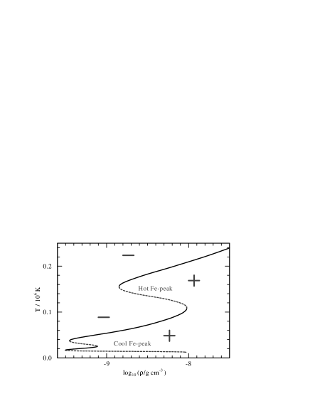
Figure 4: Solution of Eq. (23) in the $\rho$-$T$ plane. The sonic-point conditions for an optically thick wind, i.e. $\kappa_{\rm Ross}=\kappa_{\rm crit}$ with outward increasing $\kappa_{\rm Ross}$, are fulfilled at the solid parts of the curve around 70 kK, and above 160 kK. The Rosseland opacities are taken from the OPAL opacity tables. From Gräfener & Hamann.

3.3 Hydrodynamic optically thick wind models

Gräfener & Hamann (2005) included the OPAL Fe-peak opacities of the ions Fe ix–xvii in more sophisticated models that treat the full set of non-LTE population numbers in combination with the radiation field in the co-moving frame (CMF). Combining these models with the equations of hydrodynamics, Gräfener & Hamann obtained a self-consistent model for the WC5 star WR 111. The resulting wind acceleration and Fe-ionisation structure are depicted in Fig. 5. $g_{\rm rad}$ was obtained from an integration of the product of opacity and flux over frequency (see Eq. 21). Wind clumping was treated in the optically thin (“micro”) clumping approach (see Sect. 8.1). With a mass-loss rate of $\dot{M}=10^{-5.14}\,M_{\odot}/{\rm yr}$ and terminal wind velocity of $v_{\infty}=2010\,{\rm km}/{\rm s}$, the observed spectrum was also reproduced, although the electron scattering wings highlighted that the assumed clumping factor of $D=50$ was rather (too) large given that WC stars generally seem to have clumping factors of the order of $D=10$, as determined from electron scattering wings (Hillier 1991; Hamann & Koesterke 1998). The models might therefore underestimate the mass loss rate by a factor of $\sqrt{5}$. This is likely due to the omission of opacities of intermediate-mass elements, such as Cl, Ne, Ar, S, and P, which according to Monte Carlo models may account for up to half of the total line acceleration in the outer wind (Vink et al. 1999).

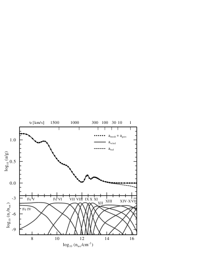
Figure 5: Top panel: the radiative acceleration of the Gräfener & Hamann (2005) WC5 star model WR 111 (expressed in units of the local gravity). The wind acceleration $g_{\mathrm{wind}}$ due to radiation and gas pressure balances the mechanical and gravitational acceleration $g_{\mathrm{mech}}+g_{\mathrm{grav}}$. Bottom panel: the Fe-ionisation structure.

4 VMS and the transition between optically thin and thick winds

There are many uncertainties in the quantitative mass-loss rates of both VMS as well as canonical 20-60 $M_{\odot}$ massive stars. One reason is related to the role of wind clumping, which will be discussed later, but there are also uncertainties related to modelling techniques. Nevertheless, arguably the most pressing uncertainty is actually still qualitative! Do VMS winds become optically thick in Nature? And if so, would this lead to an accelerated increase of $\dot{M}$? And if so, at what point does the transition occur?

4.1 Analytic derivation of transition mass-loss rate

As hydrostatic equilibrium is a good approximation for the subsonic part of the wind the terms on the right-hand side of Eq. 2 cancel each other. In the supersonic portion of the wind the gas pressure gradient becomes small, and through multiplying Eq. 2 by $4\pi r^{2}$, it reads:

$$4\pi\rho r^{2}vdv=4\pi r^{2}(g_{\rm rad}-g)dr.$$ (25)

Employing the mass-continuity equation, one obtains

$$\dot{M}dv=4\pi GM(\Gamma(r)-1)\rho dr.$$ (26)

Where $\Gamma(r)$ the Eddington factor with respect to the total flux-mean opacity $\kappa_{\rm F}$: $\Gamma(r)=\frac{\kappa_{\rm F}L}{4\pi cGM}$. Using the wind optical depth $\tau=\int_{r_{s}}^{\infty}\kappa_{\rm F}\rho\,{\rm d}r$, one obtains

$$\frac{\dot{M}}{L/c}dv=\kappa_{\rm F}\rho\frac{\Gamma-1}{\Gamma}dr=\frac{\Gamma-1}{\Gamma}d\tau.$$ (27)

Assuming hydrostatic equilibrium below the sonic point, in integral form this becomes:

$$\int_{0}^{v_{\infty}}\frac{\dot{M}}{L/c}dv=\frac{\dot{M}v_{\infty}}{L/c}=\int_{r_{\rm S}}^{\infty}\frac{\Gamma-1}{\Gamma}d\tau\simeq\tau_{\rm S}.$$ (28)

Where it is assumed that $\Gamma$ is significantly larger than one in the supersonic region, such that the factor $\frac{\Gamma-1}{\Gamma}$ becomes close to unity, and

$$\dot{M}v_{\infty}=\frac{L}{c}\tau.$$ (29)

Vink & Gräfener (2012) derived a condition for the wind efficiency number $\eta$:

$$\eta=\frac{\dot{M}v_{\infty}}{L/c}=\tau=1.$$ (30)

The key point is that one can employ the unique condition $\eta=\tau=1$ right at the transition from optically thin O-star winds to optically-thick WR winds. In other words, if one were to have a data-set containing luminosities for O and WR stars, the transition mass-loss rate $\dot{M}_{\rm trans}$ is obtained by simply considering the transition luminosity $L_{\rm trans}$ and the terminal velocity $v_{\infty}$ representing the transition point from O to WR stars:

$$\dot{M}_{\rm trans}=\frac{L_{\rm trans}}{v_{\infty}c}$$ (31)

This transition point can be obtained by purely spectroscopic means, independent of any assumptions regarding wind clumping.

As $\Gamma=g_{\rm rad}/g$ is expected to be connected to the ratio $(v_{\infty}+v_{\rm esc})/v_{\rm esc}=v_{\infty}/v_{\rm esc}+1$, and $f\simeq\frac{\Gamma-1}{\Gamma}$, Vink & Gräfener followed a model-independent approach, adopting $\beta$-type velocity laws, as well as full hydrodynamic wind models, computing the integral $\tau=\int_{r_{s}}^{\infty}\kappa\rho\,{\rm d}r$ numerically using the flux-mean opacity $\kappa_{\rm F}(r)$. The mean opacity $\kappa_{F}$ follows from the resulting radiative acceleration $g_{\rm rad}$

$$g_{\rm rad}(r)=\kappa_{F}(r)\frac{L}{4\pi cr^{2}}.$$ (32)

Whilst $g_{\rm rad}$ follows from the prescribed density $\rho(r)$ and velocity structures $v(r)$ – via the equation of motion:

$$v\frac{{\rm d}v}{{\rm d}r}=g_{\rm rad}-\frac{1}{\rho}\frac{{\rm d}p}{{\rm d}r}-\frac{GM}{r^{2}},$$ (33)

where a grey temperature structure can be assumed to compute the gas pressure $p$. The sole assumption entering this analysis is that the winds are radiatively driven. The resulting mean opacity $\kappa_{F}$ thus captures all physical effects that could affect the radiative driving, including clumping and porosity. The obtained values for the correction factor is 0.6 $\pm$ 0.2. The transition between O and WR spectral types should in reality occur at:

$$\dot{M}=f\frac{L_{\rm trans}}{v_{\infty}c}\simeq 0.6\dot{M}_{\rm trans}.$$ (34)

There is a transition between O and WR spectral types. The spectroscopic transition for spectral subtypes O4-6If+ occurs at $\log(L)=6.05$ and $\log(\dot{M}_{\eta=1}/\mbox{$M_{\odot}{\rm yr}^{-1}$})=-4.95$. This is the transition mass-loss rate for the Arches cluster. The only remaining uncertainties are due to uncertainties in the terminal velocity and the stellar luminosity $L$, with potential errors of at most $\sim$40%, and several factors lower than the order-of-magnitude uncertainties in mass-loss rates resulting form clumping and porosity.

4.2 Models close to the Eddington limit

Figure 6: Mass-loss predictions versus the Eddington parameter $\Gamma$ – divided by $M^{0.7}$. Symbols correspond to models of different mass ranges (Vink et al. 2011).

The predictions of the O star recipe of Vink et al. (2000) and Eq. (14) are only valid for objects at a sufficient distance from the Eddington limit, with $\Gamma$ $\leq$ 0.5. There are two regimes where this is no longer the case: (i) stars that have formed with large initial masses and luminosities, i.e. very massive stars (VMS) with $M$ $>$ 100 $M_{\odot}$, and (ii) less extremely luminous “normal” stars that approach the Eddington limit when they have evolved significantly. Examples of the latter category are LBVs and classical WR stars.

For LBVs, Vink & de Koter (2002) and Smith et al. (2004) showed with Monte Carlo computations that the mass-loss rate increases more rapidly than Eq. (14) indicates. This implies that not only does the mass-loss rate increase when the Eddington limit is approached, but the mass-loss rate increases more strongly, which leads to a positive feedback effect on the total mass lost over time. For VMS, Vink et al. (2011) discovered a kink in the slope of the mass-loss vs. $\Gamma$ relation at the transition from optically thin O-type to optically thick WR-type winds. Bestenlehner et al. (2014) performed a homogeneous spectral analysis of $>$ 60 Of-Of/WN-WNh stars in 30 Doradus, and confirmed the kink empirically.

Figure 6 depicts mass-loss predictions for VMS as a function of the Eddington parameter $\Gamma$ from Monte Carlo modelling. For ordinary O stars with “low” $\Gamma$ the $\dot{M}$ $\propto$ $\Gamma^{x}$ relationship is shallow, with $x$ $\simeq$2. There is a steepening at higher $\Gamma$, where $x$ becomes $\simeq$5. Here the optical depths and wind efficiencies exceed unity.

5 Predictions for low metallicity $Z$ and Pop III stars

For objects in a $Z$-range representative for the observable Universe with $Z/\mbox{$Z_{\odot}$}$ $>$ 1/100, Monte Carlo mass-loss predictions were provided by Vink et al. (2001). Extending the predictions to extremely low $Z/\mbox{$Z_{\odot}$}$ $<$ $10^{-2}$, $\dot{M}$ is still expected to drop until the winds reach a point where they become susceptible to ion-decoupling and multi-component effects (Krticka et al. 2003). In order to maintain a one-fluid wind model is by increasing the Eddington factor – by pumping up the stellar mass and luminosity.

For the case of Pop III stars with truly “zero” metallicity, i.e. only H and He present, it seems unlikely that these objects develop stellar winds of significant strength (Kudritzki et al. 2002; Muijres et al. 2012b). However, other physical effects may contribute to the driving. Interesting possibilities include stellar rotation and pulsations, although pure vibration models for Pop III stars also indicate little mass loss via pulsations alone (Baraffe et al. 2001). Perhaps a combination of several effects could result in large mass loss close to the Eddington limit. Moreover, we know that even in the present-day Universe a significant amount of mass is lost in LBV type eruptions, potentially driven by continuum radiation pressure, which might be also relevant for the First Stars (Vink & de Koter 2005; Smith & Owocki 2006).

Despite the fact that the first generations of massive stars start their evolutionary clocks with fewer metals, as the First Stars may be highly luminous and/or rapidly rotating, it is not inconceivable that they enrich their atmospheres with nitrogen and carbon (Meynet et al. 2006), thereby inducing a stellar wind (Vink 2006).

In a first attempt to investigate the effects of self-enrichment on the total wind strength, Vink & de Koter (2005) performed a pilot study of WR mass loss versus $Z$. The prime interest in WR stars here is that these objects, especially those of WC subtype, show the products of core burning in their outer atmospheres.

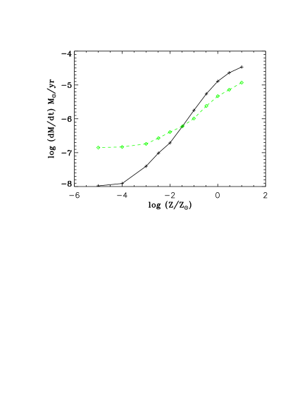
Figure 7: Monte Carlo WR mass-loss predictions as a function of $Z$. The dark line represents the late-type WN stars, whilst the lighter dashed line shows the results for late-type WC stars. The slope for the WN models is similar to the predictions for OB-supergiants, whereas the slope is shallower for WC stars. At low $Z$, the slope becomes smaller, flattening off entirely at $Z/\mbox{$Z_{\odot}$}$ $=$ $10^{-3}$. The computations are from Vink & de Koter (2005).

The reasoning behind the assertion that WR winds may not be $Z$-dependent was that WR stars enrich themselves by burning He into C, and it could be the large C-abundance that is the most relevant ion for the WC wind driving, rather than the sheer number of Fe lines. Figure 7 shows that despite the fact that the C ions overwhelm the amount of Fe, both late-type WN (dark line) and WC (light line) show a strong $\dot{M}$-$Z$ dependence, basically because Fe has such a complex electronic structure.

The implications of Fig. 7 are two-fold. First, WR mass-loss rates decrease steeply with $Z$. This may be of key relevance for black hole formation and the progenitor evolution of long duration GRBs. The collapsar model of MacFadyen & Woosley (1999) requires a rapidly rotating stellar core prior to collapse, but at solar metallicity stellar winds are expected to remove the bulk of the core angular momentum (Zahn 1992). The WR $\dot{M}$-$Z$ dependence from Fig. 7 provides a route to maintain rapid rotation, as the winds are weaker at lower $Z$ prior to final collapse.

The second point is that mass loss is no longer expected to decrease when $Z/\mbox{$Z_{\odot}$}$ falls below $\sim$$10^{-3}$ (due to the dominance of driving by carbon lines). This suggests that once massive stars enrich their outer atmospheres, radiation-driven winds might still exist, even if stars started their lives with extremely small amounts of metals.

Whether the mass-loss rates are sufficiently high to alter the evolutionary tracks of the First Stars remains to be seen, but it is important to keep in mind that the mass-loss physics does not only quasi-linearly depend on $Z$, but that other factors, such as the proximity to the $\Gamma$ limit, should also be considered.

6 Luminous Blue Variables

6.1 What is an LBV?

Luminous Blue Variables represent a short-lived ($\sim 10^{4}-10^{5}$ years) phase of massive star evolution during which the objects are subjected to humongous changes in their stellar radii by about an order of magnitude. They come in two flavors. The largest population of $\sim$30 LBVs in the Galaxy and the Magellanic Clouds is that of the S Doradus variables with magnitude changes of 1-2 magnitudes on timescales of years to decades (Humphreys & Davidson 1994). These are the characteristic S Dor variations, represented by the dotted horizontal lines in Fig. 8. The general understanding is that the S Dor cycles occur at approximately constant bolometric luminosity (which has yet to be proven) – principally representing temperature variations. The second type of LBV instability involves objects that show truly giant eruptions with magnitude changes of order $3-5$ during which the bolometric luminosity most certainly increases. In the Milky Way it is only the cases of P Cygni and Eta Carina which have been noted to exhibit such giant outbursts.

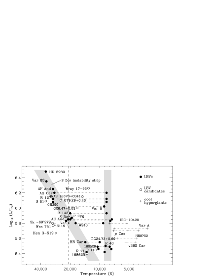
Figure 8: The LBVs in the Hertzsprung-Russell diagram. The slanted band running from 30 kK at high $L/\mbox{$L_{\odot}$}$ to 15 kK at lower luminosity is the S Dor instability strip. The vertical band at a temperature of $\sim$ $8\,000$ K represents the position of the LBVs “in outburst”. The vertical line at 21 000 K is the position of the observed bi-stability jump (Lamers et al. 1995). Adapted from Vink (2012) and Smith et al. (2004).

Whether these types of variability occur in similar or distinct objects is not yet clear, but in view of the “unifying” properties of the object P Cygni it is rather probable that the S Dor variables and giant eruptors are subject to the same type of instabilities near the Eddington limit (see Vink 2012).

Figure 9: Pseudo-photosphere formation in a relatively low mass LBV with a high $L/M$ ratio. The difference in inner (dashed) and apparent temperature (representative for the size of the computed pseudo-photosphere) is plotted against the stellar mass. These computations have been performed for a constant luminosity of log $L/\mbox{$L_{\odot}$}$ $=$ $5.7$. The mass is gradually decreased whilst the LBV approaches the Eddington limit: the apparent temperature drops as a result of the lower effective gravity, and the higher mass loss results in the formation of a pseudo-photosphere (Smith et al. 2004).

6.2 Do LBVs form pseudo-photospheres?  

Although it appears that the photospheric temperatures of the objects in Fig. 8 change during HRD transits, there is an alternative possibility that the underlying star does not change its actual temperature but that the star undergoes changes in mass-loss properties instead. The second case is normally referred to as the formation of a “pseudo-photosphere” resulting from the formation of an optically thick wind.

Eta Car’s outstanding wind density with $\dot{M}$$\sim 10^{-3}$$M_{\odot}{\rm yr}^{-1}$(Hillier et al. 2001) places $R(\mbox{$\tau_{\rm Ross}$}=2/3)$ at 80% of the terminal velocity, impeding any derivation of the hydrostatic radius, but it is not yet clear whether the general LBV population of S Dor variables have $\dot{M}$ values high enough to produce pseudo photospheres.

As a result of enhanced mass loss during maximum it is hypothetically possible to form a pseudo-photosphere. Until the late 1980s this was the leading idea to explain the colour changes of S Dor variables. Using more advanced non-LTE model atmosphere codes, Leitherer et al. (1989) and de Koter et al. (1996) predicted colours based on empirical LBV mass-loss rates that are not red enough to make an LBV appear cooler than the temperature of its underlying surface. Despite the proximity of LBVs to the Eddington limit, current consensus is that LBV winds are generally not sufficiently optically thick.

Figure 9 shows the potential formation of an optically thick wind for a relatively low-mass (with high $L/M$) LBV in close proximity to the bi-stability jump (Pauldrach & Puls 1990; Vink & de Koter 2002; Groh & Vink 2011). The size of the temperature difference (dashed vs. solid) is a proxy for the extent of the pseudo-photosphere. The figure demonstrates that for masses in the range 15-25 $M_{\odot}$ and fixed luminosity, the winds remain optically thin, but when the stellar mass approaches values as low as 10 $M_{\odot}$, and the star enters the mass-loss regime near the Eddington limit, the photospheric scale-height blows up, which results in the formation of a pseudo-photosphere.

6.3 Winds during S Doradus variations.  

Although most S Dor variables have been subject to photometric monitoring, only a few have been analysed in sufficient detail to understand the driving mechanism of their winds. Mass-loss rates are of the order of $10^{-3}$ - $10^{-5}$ $M_{\odot}{\rm yr}^{-1}$, whilst terminal wind velocities are in the range $\sim 100-500\,\mbox{${\rm km}\,{\rm s}^{-1}$}$. Obviously, these values vary with $L$ and $M$, but there are indications that the mass loss varies as a function of $T_{\rm eff}$ when the S Dor variables transit the upper HRD on timescales of years, providing an ideal laboratory for testing the theory of radiation-driven winds.

The Galactic LBV AG Car is one of the best monitored and analysed S Dor variables. Vink & de Koter (2002) predicted $\dot{M}$ rises in line with radiation-driven wind models for which the $\dot{M}$ variations are attributable to ionisation shifts of Fe. Sophisticated non-LTE spectral analysis have since confirmed these predictions (Groh et al. 2011; Groh & Vink 2011).

It is relevant to mention here that this variable wind concept (wind bi-stability; see also Pauldrach & Puls 1990) has been suggested to be responsible for circumstellar density variations inferred from modulations in radio light-curves and H$\alpha$ spectra of supernovae (Kotak & Vink 2006; Trundle et al. 2008). However most stellar evolution models would have predicted massive stars with $M$ $\geq$ 25 $M_{\odot}$ to explode at the end of the WR phase, rather than after the LBV phase. The implications could be gigantic, impacting our most basic understanding of massive star death in the Universe (see Smith’s Chapter 8).

6.4 Super-Eddington winds

Whilst during “quiet” phases, LBVs may lose mass via ordinary line-driving, some objects, like Eta Car also seem to be subject to phases of more extreme mass loss. For instance, the giant eruption of $\eta$ Car with a cumulative loss of $\sim$10 $M_{\odot}$ between 1840 and 1860 (Smith et al. 2003) which resulted in the Homunculus nebula corresponds to $\mbox{$\dot{M}$}\approx$ 0.1-0.5 $M_{\odot}{\rm yr}^{-1}$, which is a factor of 1000 larger than that expected from line-driven wind models for an object of that luminosity.

Shaviv (1998) and Owocki et al. (2004) studied the theory of porosity-moderated continuum driving in objects that formally exceed the Eddington limit. It is possible that continuum-driven winds in super-Eddington stars reach mass-loss rates close to the photon tiring limit, $\mbox{$\dot{M}$}_{\rm tir}=\mbox{$L_{\ast}$}$/ $(G\mbox{$M_{\ast}$}/\mbox{$R_{\ast}$})$, which could result in a stagnating flow that may lead to spatial structure (van Marle et al. 2008). However, it should be noted that alternatively, wind clumping may be the result of other instabilities, possibly related to the presence of the Fe opacity peak (Cantiello et al. 2009; Gräfener et al. 2012; Gräfener & Vink 2013; Glatzel et al. 1993), especially for objects approaching the $\Gamma$-limit.

The general equation of motion for a stellar wind (ignoring gas pressure) is given by:

$$v\Bigl{(}1-\frac{a^{2}}{v^{2}}\Bigr{)}\frac{{\rm d}v}{{\rm d}r}\simeq g_{\rm grav}(r)+g_{\rm rad}(r)=-\frac{GM}{r^{2}}(1-\Gamma(r)).$$ (35)

At the sonic point, $r_{s}$: $v=a$, and thus $g_{\rm rad}=-g_{\rm grav}$ implying $\Gamma(r_{s})=1$. Thus, $\Gamma(r)$ must be $<1$ below the sonic point and $\Gamma(r)$ must be $>1$ above the sonic point. An accelerating wind solution thus implies an increasing opacity$\frac{{\rm d}\bar{\kappa}}{{\rm d}r}|_{s}>0$ (given that $\Gamma(r)=\frac{\bar{\kappa}(r)L_{\ast}}{4\pi GMc}$).

If, on the other hand, the entire atmosphere is super-Eddington, i.e. $\Gamma(r)>1$ throughout the atmosphere, continuum driving might nonetheless become possible. The reason is that when atmospheres exceed the Eddington limit, instabilities may arise which could make them clumpy: outward travelling photons may avoid regions of enhanced density, which means that the medium may behave in a porous manner, leading to a lower $g_{\rm rad}$. This means that the effective Eddington parameter can drop below unity. However, further out in the wind, the clumps become optically thinner as a result of expansion, and the porosity effect decreases. $\Gamma_{\rm eff}^{\rm cont}$ can now become larger than unity. In other words, a wind solution with $\Gamma_{\rm eff}^{\rm cont}$ crossing unity is feasible, even when the stars are formally above the Eddington limit.

Owocki et al. (2004) expressed the effective opacity in terms of the so-called porosity length (see Sect. 8). They showed that $\dot{M}$ might become substantial when the porosity length is of the order of the pressure scale height $H$. Owocki et al. developed the concept of a power-law distributed porosity length (in analogy to CAK-type the line-strength distribution function), and showed that even the gigantic mass-loss rate during Eta Car’s giant eruption might be explained by some form of radiative driving.

7 Observed wind parameters

Radiation-driven wind models can provide predictions for two global wind parameters: the mass-loss rate, $\dot{M}$, and the terminal velocity, $v_{\infty}$. Most studies rely on the assumption of a smooth wind. The mass-loss rate then follows from the continuity equation (Eq. 1), and most diagnostics are based on a wind model with a prescribed $\beta$-type velocity field.

A useful concept involves the optical-depth invariant $Q$ parameter (Puls et al. 1996), where $Q_{\rm res}$ can be utilised for resonance lines with line opacity $\propto\rho$. Alternatively, recombination is a 2-body process and $Q_{\rm rec}$ is useful for recombination based line processes such as H_α which thus have opacities $\propto\rho^{2}$,

$$Q_{\rm res}=\frac{\mbox{$\dot{M}$}}{\mbox{$R_{\ast}$}\mbox{$v_{\infty}$}^{2}},\qquad\qquad Q_{\rm rec}=\frac{\mbox{$\dot{M}$}}{(\mbox{$R_{\ast}$}\mbox{$v_{\infty}$})^{1.5}}.$$ (36)

Most diagnostics rely on the use of non-LTE model atmospheres. Stellar and wind parameters, such as $\dot{M}$ can be determined by fitting resonance and recombination lines simultaneously. Smooth wind models constitute the ideal case, but the optical depth invariant $Q_{\rm rec}$ as defined in Eq. 36 can easily be modified for the case that the winds are clumped (Sect. 8, Eq. 46).

A more detailed discussion of the various methods to derive wind parameters is given in Puls et al. (2008). The most common line profiles in a stellar wind are (i) UV P Cygni profiles with a blue absorption trough and a red emission peak, and (ii) optical emission lines (such as H$\alpha$). These line shapes are caused by different population mechanisms of the upper energy level of the transition. In a P Cygni scattering line, the upper level is populated by the balancing act between absorption from and spontaneous decay to the lower level. An emission line is formed if the upper level is populated by recombinations from above (see however Puls et al. 1998; Petrov et al. 2014 for the formation of P Cygni H$\alpha$ lines in the cooler BA supergiants).

7.1 Ultraviolet P Cygni Resonance lines

P Cygni lines may be used to determine the velocity field in stellar winds, and in particular $v_{\infty}$. H_α is generally utilised to derive $\dot{M}$ (or $Q_{\rm rec}$). UV P-Cygni lines from hot stars (e.g. C iv and P v) are usually analysed by means of the Sobolev optical depth:

$$\mbox{$\tau_{\rm Sob}$}(r)=\frac{\frac{\pi e}{m_{\rm e}c}f\mbox{$n_{\rm l}$}(r)\lambda}{\mbox{${\rm d}v/{\rm d}r$}}\frac{\mbox{$R_{\ast}$}}{\mbox{$v_{\infty}$}},$$ (37)

where $f$ is the oscillator-strength and $n_{\rm l}$ the lower occupation number of the transition. Relating the occupation number, $n_{\rm l}$, to the density:

$$\mbox{$\tau_{\rm Sob}$}(r)=\frac{1}{r^{2}v\mbox{${\rm d}v/{\rm d}r$}}\,E(r)q(r)\,\frac{\mbox{$\dot{M}$}}{\mbox{$R_{\ast}$}\mbox{$v_{\infty}$}^{2}}\,\frac{(\pi e^{2})/(m_{\rm e}c)}{4\pi m_{\rm H}}\,\frac{A_{\rm k}}{1+4Y}\,f\lambda,$$ (38)

where $E$ is the excitation factor of the lower level, $q$ the ionisation fraction, $A_{\rm k}$ the abundance of the element, and $Y$ the He abundance. This quantity is invariant with respect to $Q_{\rm res}=\mbox{$\dot{M}$}/(\mbox{$R_{\ast}$}\mbox{$v_{\infty}$}^{2})$ (see Eq. 36) as long as the ground-state population is proportional to the density $\rho$. Thus, $\dot{M}$ can be derived from resonance line P Cygni profiles when the ionisation fraction is known. Most P Cygni lines however are saturated and mass-loss rate derivations become unfeasible, such that only lower limits on $\dot{M}$ can be determined.

UV resonance lines have been considered relatively clean from clumping effects, but this might not be the case if porosity effects become important.

7.2 The H$\alpha$ recombination emission line

The most oft-used diagnostics to derive $\dot{M}$ for O-star winds involves H_α, for which there is hardly any uncertainty due to ionisation. The H_α opacity scales with $\rho^{2}$, and

$$\mbox{$\tau_{\rm Sob}$}(r)\propto\frac{\mbox{$\dot{M}$}^{2}}{(\mbox{$R_{\ast}$}\mbox{$v_{\infty}$})^{3}}\frac{b_{2}(r)}{r^{4}v^{2}\mbox{${\rm d}v/{\rm d}r$}},$$ (39)

i.e., the scaling invariant quantity is now $Q_{\rm rec}^{2}$ (Eq. 36), and $b_{2}$ is the non-LTE departure coefficient of $n_{2}$.

The challenge with H_α concerns its $\rho^{2}$ dependence. Any notable inhomogeneity will necessarily result in an $\dot{M}$ overestimate if clumping is neglected in the analysis. An advantage is the fact that H_α remains optically thin in the main part of the emitting wind, such that porosity effects can be neglected (which is not the case for UV resonance lines).

7.3 Radio and (sub)millimetre continuum emission

A somewhat different approach to measure mass-loss rates is to utilize long wavelength radio and (sub)millimetre continua. In fact this approach may lead to the most accurate results, as they are model-independent. The basic concept is to measure the excess wind flux over that from the stellar photosphere. This excess flux is emitted by free-free and bound-free processes. The reason the excess flux becomes more important at longer (sub)-mm/radio wavelengths is due to the $\lambda^{2}$ dependence of the opacities.

Following Wright & Barlow (1975), Panagia & Felli (1975), and Lamers & Cassinelli (1999), the dominant free-free opacity (in units of cm^-1) at frequency $\nu$ can be written as:

$$\kappa_{\nu}\propto n_{\rm i}\,n_{\rm e}\,g_{\nu}\,(\frac{1}{\nu^{2}})\propto{\frac{\dot{M}}{\mbox{$v_{\infty}$}}}^{2}\,(\frac{1}{r^{4}})\,g_{\nu}\,(\frac{1}{\nu^{2}}),$$ (40)

in cm^-3, and $g_{\nu}$ is the Gaunt factor for free-free emission. For an isothermal wind and frozen-in ionisation, $\bar{z}$ (the mean value of the atomic charge) and $\mu_{\rm e}$ and $\mu_{\rm i}$ remain constant, and:

$$\kappa_{\nu}\propto{g_{\nu}\lambda^{2}\rho^{2}},$$ (41)

which increases with $\lambda$ and $\rho$. As the continuum becomes optically thick in the wind in free-free opacity the emitting wind volume increases as a function of $\lambda$, leading to the formation of a radio photosphere where the the radio emission dominates the stellar photospheric emission. For a typical O supergiant this occurs at about 100 stellar radii. At such large distances the outflow reaches its terminal wind velocity and an analytic solution of the radiative transfer problem becomes possible:

$$F_{\nu}\propto\Bigl{(}\frac{\mbox{$\dot{M}$}}{\mbox{$v_{\infty}$}}\Bigr{)}^{4/3}\,\frac{\bigl{(}\nu g_{\nu}\bigr{)}^{2/3}}{d^{2}},$$ (42)

where $F_{\nu}$ is the observed radio flux measured in Jansky, $\dot{M}$ in units of $M_{\odot}{\rm yr}^{-1}$, $v_{\infty}$ in ${\rm km}\,{\rm s}^{-1}$, distance $d$ to the star in kpc and frequency $\nu$ in Hz. Thus, the spectral index of thermal wind emission is close to 0.6.

8 Wind clumping

H$\alpha$ and long-wavelength continuum diagnostics depend on the density squared, and are thus sensitive to clumping, whereas UV P Cygni lines such as Pv are insensitive to clumping, as they depend linearly on density. In the canonical optically thin (micro-clumping) approach the wind is divided into a portion of the wind that contains all the material with a volume filling factor $f$ (the reciprocal of the clumping factor $D$), whilst the remainder of the wind is assumed to be void. In reality however, clumped winds are porous with a range of clump sizes, masses, and optical depths.

Wind clumping has been extensively discussed for canonical 20-60 $M_{\odot}$ O-type stars and WR stars in a dedicated clumping workshop (Hamann et al. 2008). Here one may also find studies of X-ray observations (see also Cohen et al. 2014 and references therein for more recent work).

8.1 Optically thin clumping (“micro-clumping”)

The general concept of optically-thin micro clumping is simply based on the assumption that the wind is made up of large numbers of small-scale density clumps. Largely motivated by the results from hydrodynamic simulations including the line-deshadowing instability (LDI; see Owocki’s Chapter 5), the inter-clump gas is usually assumed to be void. The average density $\mbox{$\langle\rho\rangle$}=\mbox{$\dot{M}$}/(4\pi r^{2}v$) is given by:

$$\mbox{$\langle\rho\rangle$}=f\rho_{C},\quad\mbox{$\langle\rho^{2}\rangle$}=f(\rho_{C})^{2}$$ (43)

where $\rho_{C}$ is the density inside the over-dense clumps, and $\langle\rho^{2}\rangle$ is the mean of the squared density. Thus, the clumping factor:

$$D=\mbox{$\langle\rho^{2}\rangle$}/\mbox{$\langle\rho\rangle$}^{2}\quad\Rightarrow\quad D=f^{-1}\quad\mbox{and}\quad\rho_{C}=D\mbox{$\langle\rho\rangle$},$$ (44)

measures the clump over-density. As the inter-clump space is assumed to be void, matter is only present inside the clumps, with density $\rho_{C}$, and with its opacity given by $\kappa=\kappa_{C}(D\mbox{$\langle\rho\rangle$})$, where $C$ represents the quantities inside the clump. Optical depths may be calculated via $\tau=\int\kappa_{C}(D\mbox{$\langle\rho\rangle$})f{\rm d}r$ with a reduced path length $(f{\rm d}r)$ as to correct for the volume where clumps are actually present.

The formulation is only correct as long as the clumps are optically thin, and optical depths may be expressed by a mean opacity $\bar{\kappa}$:

$$\bar{\kappa}=\kappa_{C}(D\mbox{$\langle\rho\rangle$})f=\frac{1}{D}\kappa_{C}(D\mbox{$\langle\rho\rangle$}).$$ (45)

Thus, for processes that are linearly dependent on density, the mean opacity of a clumped medium is exactly the same as for a smooth wind, whilst for processes that scale with the density squared, mean opacities are enhanced by the clumping factor D.

It should be noted that processes described by the optically thin micro-clumping approach do not depend on clump size nor geometry, but only the sheer clumping factor. The enhanced opacity for $\rho^{2}$ dependent processes implies that $\dot{M}$ derived by such diagnostics are a factor of $\sqrt{D}$ lower than older mass-loss rates derived with the assumption of smooth winds. As a result, the optical depth invariant, $Q_{\rm rec}$ (see Eq. 36) transforms into:

$$Q_{\rm rec}=\frac{\mbox{$\dot{M}$}\sqrt{D}}{(\mbox{$R_{\ast}$}\mbox{$v_{\infty}$})^{1.5}}.$$ (46)

Note that also for the case of thermal radio and (sub)-mm continuum emission the scaling invariant is proportional to $\mbox{$\dot{M}$}/\mbox{$R_{\ast}$}^{1.5}$, i.e. very similar to $Q_{\rm rec}$ for optical emission lines, such as H$\alpha$. Abbott et al. (1981) studied the effects of clumping on the wind radio emission as a function of the volume filling factor and the density ratio between clumped and inter-clump material. For the standard assumption of vanishing inter-clump density, Abbott et al. showed that the radio flux may be a factor $f^{-2/3}$ larger than that from a smooth wind with the same $\dot{M}$. In other words, using Eq. 42, it can be noted that radio mass-loss rates derived from clumped winds must also be lower than those derived from smooth winds.

8.2 The P v problem

Due to the very low cosmic abundance of phosphorus (P), the P v doublet remains unsaturated, even when P⁺⁴ is dominant. This allows for a direct estimate of the product $\dot{M}$$\langle q\rangle$, where $\langle q\rangle$ is a spatial average of the ion fraction. Unfortunately, $\langle q\rangle$ estimates for a given resonance line are uncertain due to shocks and associated X-ray ionisation. Empirical determination of ionisation fractions is normally not feasible, as resonance lines from consecutive ionisation stages are not generally available. Nevertheless, for P v, insight is gained from FUSE data: for those O-stars in a certain $\mbox{$\langle q\rangle$}\simeq 1$ region, the P v line should provide an accurate estimate of $\dot{M}$, as the pure linear character with $\rho$ makes it clumping independent.

Fullerton et al. (2006) selected a large sample of O-stars, which also had $\rho^{2}$ (from H$\alpha$/radio) estimates available, and compared both $\rho$-linear UV and $\rho$-quadratic dependent methods. They found enormous discrepancies, with a median $\dot{M}$($\rho^{2}$)/($\dot{M}$(P v)$\langle q\rangle$) = 20 in mid-O supergiants, implying an extreme clumping factor D $\simeq$ 400 if the winds could indeed be treated in an optically thin (micro-clumping) approach (see also Bouret et al. 2003).

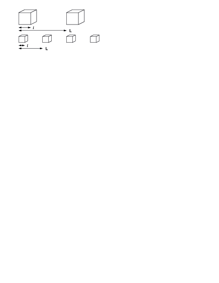
Figure 10: Schematic explanation of porosity, involving a notable difference between the volume filling fraction f (and its reciprocal clumping factor $D=1/f$), which is the same for the top and bottom case, and the separation of the clumps $L$, which is larger in the top case than the bottom case (from Muijres et al. 2011).

8.3 Optically thick clumping (“macro”-clumping)

With studies yielding clumping factors ranging from $D$ up to 400, one may wonder whether a pure micro-clumping analysis is physically sound. Most of the atmospheric codes only consider density variations, but hydrodynamic simulations also reveal strong velocity changes inside the clumps. Most worrisome is probably the assumption that all clumps are assumed to be optically thin.

Within the optically thin approach, a clump has a size smaller than the photon mean free path. However, in an optically thick clump, photons may interact with the gas several times before they escape through the inter-clump gas. Whether a clump is optically thin or thick depends on the abundance, ionisation fraction, and cross-section of the transition.

For optically thick clumps, photons care about the distribution, the size and the geometry of the clumps (see Fig. 10). The conventional description of macro-clumping is based on a clump size, $l(r)$, and an average spacing of a statistical distribution of clumps, $L(r)$, which are related to $f$:

$$f=\bigl{(}\frac{l}{L}\bigr{)}^{3}=\frac{1}{D}.$$ (47)

Following Eq. 45, the optical depth across a clump of size $l$ and opacity $\kappa_{C}$ becomes:

$$\tau_{C}=\kappa_{C}l=\bar{\kappa}Dl=\bar{\kappa}\frac{L^{3}}{l^{2}}=\bar{\kappa}h,$$ (48)

with mean opacity $\bar{\kappa}$ (Eq. 45) and porosity length $h=L^{3}/l^{2}$. The porosity length $h$ involves the key parameter to define a clumped medium, as $h$ corresponds to the photon mean free path in a medium consisting of optically thick clumps.

The effective clump cross section, i.e., the spatial cross section now corrected for the fraction of transmitted radiation, becomes:

$$\sigma_{C}=l^{2}\,(1-\mbox{${\rm e}$}^{-\tau_{C}}),$$ (49)

and the effective opacity becomes:

$$\kappa_{\rm eff}=n_{C}\sigma_{C}=\frac{l^{2}\,(1-\mbox{${\rm e}$}^{-\tau_{C}})}{L^{3}}=\bar{\kappa}\frac{(1-\mbox{${\rm e}$}^{-\tau_{C}})}{\tau_{C}},$$ (50)

where $n_{C}$ is the clump number density. The key point is that this very equation holds for clumps of any optical thickness! For instance, in the optically thin limit, the micro-clumping approximation is recovered: $\kappa_{\rm eff}=\bar{\kappa}$, which depends on $f$ and not on clump size or distribution. In the optically thick case, the effective opacity is indeed reduced appropriately, $\kappa_{\rm eff}=\bar{\kappa}/\tau_{C}$ = $h^{-1}$ now only depending on $h$.

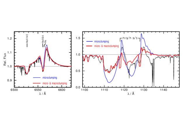
Figure 11: Porosity as a possible solution for the PV problem. Adapted from Oskinova et al. (2007).

Oskinova et al. (2007) employed the effective opacity concept in the formal integral for the line profile modelling of the O supergiant $\zeta$ Pup. Figure 11 shows that the most pronounced effect involves strong resonance lines, such as P v which can be reproduced by this macro-clumping approach – without the need for extremely low $\dot{M}$ – resulting from an effective opacity reduction when clumps become optically thick. Given that H_α remains optically thin for O stars it is not affected by porosity, and it can be reproduced simultaneously with P v. This enables a solution to the P v problem (see also Surlan et al. 2013).

However, this porosity concept was developed for continuum processes, whilst line processes may also be affected by velocity-field changes. Owocki (2008) performed LDI simulations where the line strength was described through a velocity-clumping factor. These simulations resulted in a reduced wind absorption due to porosity in velocity space, which has been termed “vorosity”. The issue with explaining a reduced P v line-strength through vorosity is that one needs to have a relatively large number of substantial velocity gaps, which does not easily arise from the LDI simulations. In any case, there is still a need to study scenarios including both porosity and vorosity, as well as how they interrelate (Sundqvist et al. 2012).

8.4 Quantifying the number of clumps

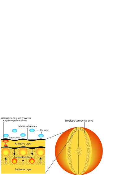
Figure 12: Cartoon of the physical processes involved in sub-surface convection. Acoustic and gravity waves are emitted in the convective zone, and travel through the radiative layers, reaching the stellar surface, thereby inducing density and velocity fluctuations. In this picture, clumping starts at the wind base. From Cantiello et al. (2009).

In the traditional view of line-driven winds of O-type stars via the CAK theory and the associated LDI, clumping would be expected to develop in the wind when the wind velocities are large enough to produce shocked structures. For typical O star winds, this is thought to occur at about half the terminal wind velocity at about 1.5 stellar radii.

Various observational indications, involving the existence of linear polarisation (e.g. Davies et al. 2005) as well as radial dependent spectral diagnostics (Puls et al. 2006) however show that clumping must already exist at very low wind velocities, and more likely arise in the stellar photosphere. Cantiello et al. (2009) suggested that waves produced by the subsurface convection zone associated with the Fe opacity peak could lead to velocity fluctuations, and possibly density fluctuations, and thus be the root cause for the observed wind clumping at the stellar surface (see Fig. 12).

Assuming the horizontal extent of the clumps to be comparable to the sub-photospheric pressure scale height $H_{\rm p}$, one may estimate the number of convective cells by dividing the stellar surface area by the surface area of a convective cell finding that it scales as ($R/H_{\rm P})^{2}$. For main-sequence O stars in the canonical mass range 20-60 $M_{\odot}$, pressure scale heights are within the range 0.04-0.24 $R_{\odot}$, corresponding to a total number of clumps 6 $\times 10^{3}-6\times 10^{4}$. These estimates may in principle be tested through linear polarisation variability, which probes wind asphericity at the wind base.

In an investigation of WR linear polarisation variability Robert et al. (1989) uncovered an anti-correlation between the wind terminal velocity and the scatter in polarisation. They interpreted this as the result of blobs that grow or survive more effectively in slow winds than fast winds. Davies et al. (2005) found this trend to continue into the regime of LBVs, with even lower $v_{\infty}$. LBVs are are thus an ideal test-bed for constraining clump properties, due to the larger wind-flow times. Davies et al. showed that over 50% of LBVs are intrinsically polarised. As the polarisation angle was found to vary irregularly with time, the polarisation line effects were attributed to wind clumping. Monte Carlo models for scattering off wind clumps have been developed by Code & Whitney (1995); Rodriguez & Magalhaes (2000); and Harries (2000), whilst analytic models to produce the variability of the linear polarisation may be found in Davies et al. (2007); Li et al. (2009); and Townsend & Mast (2011).

An example of an analytic model that predicts the time-averaged polarisation for the LBV P Cygni is presented in Fig. 13. The clump ejection rate per wind flow-time $\mathcal{N}$ is defined as ${\mathcal{N}}=\dot{N}t_{\rm fl}=\dot{N}R_{\star}/v_{\infty}$, where the clump ejection rate, $\dot{N}$, is related to $\dot{M}$ as $\dot{M}=\dot{N}N_{e}\mu_{e}m_{H}$, where $N_{e}$ is the number of electrons in each clump, and $\mu_{e}$ is the mean mass per electron. There are two regimes where the observed polarisation level can be achieved. One is where the ejection rate is low and a few very optically thick clumps are expelled; the other one is that of a very large number of clumps. These two cases can be distinguished via time resolved polarimetry. Given the relatively short timescale of the observed polarisation variability, Davies et al. argued that LBV winds consist of order thousands of clumps near the photosphere.

Nevertheless, for main-sequence O stars the derivation of wind-clump sizes from polarimetry has not yet been feasible as very high signal-to-noise data are required. LBVs however provide an excellent group of test-objects owing to the combination of higher mass-loss rates, and lower terminal wind velocities. Davies et al. (2007) showed that in order to produce the observed polarisation variability of P Cygni, the wind should consist of $\sim$ 1000 clumps per wind flow-time. In order to check whether this is compatible with the sub-surface convection scenario ultimately being the root cause for wind clumping, one would need to consider the sub-surface convective regions of an object with global properties similar to those of P Cygni. Due to the lower LBV gravity, the pressure scale height is about 4$R_{\odot}$, i.e. significantly larger than for O-type stars. As a result, the same estimate for the number of clumps drops to about 500 clumps per wind-flow time, which appears to be consistent with that derived for P Cygni from observations (see Fig. 13).

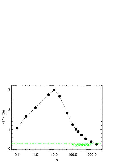
Figure 13: Time-averaged polarisation over a range of ejection rates per wind flow-time. At $\mathcal{N}\sim 20$, the optical depth per clump exceeds unity and the overall polarisation falls off (see Davies et al. 2007 for details). The observed polarisation level for the LBV P Cygni is given by the dash-dotted line. There are two ejection-rate regimes where the required polarisation level can be achieved.

8.5 Effects on mass-loss predictions

Muijres et al. (2011) studied the possible effects of both optically thin and thick wind clumping (porosity) on mass-loss predictions for O-type stars.

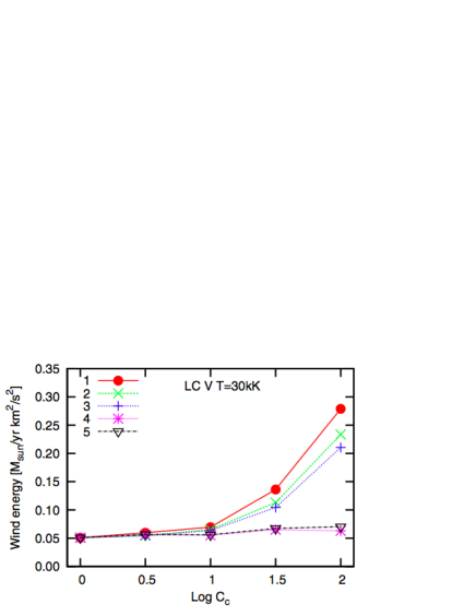
Figure 14: The effect of optically thin micro-clumping on the wind kinetic energy in Monte Carlo simulations for different clumping stratifications for 30,000 K OV-type stars. The smooth wind models have $D=1$. The numbers 1-5 refer to different clumping stratifications (see Muijres et al. 2011 for details), but clumping in the outer winds (stratifications 1 through 3) results in an increase of the kinetic wind energy due to a larger number of effective driving lines.

Because of the non-linear character of the equation of motion, the CAK solution is complex, with the physics involving instabilities due to the LDI (e.g. Owocki et al. 1988). One of the key implications of the LDI is that in hydro-dynamical simulations the time-averaged $\dot{M}$ is not anticipated to be affected by wind clumping, as it has the same average $\dot{M}$ as the smooth CAK solution. However, the shocked velocity structure and its associated density structure are expected to result in effects on the mass-loss diagnostics.

In contrast to the LDI simulations, Muijres et al. (2011) studied the effects of clumping on $g_{\rm rad}$ due to changes of the ionisation structure, as well as the effects of wind porosity, using Monte Carlo simulations. When only accounting for optically thin (micro) clumping $g_{\rm rad}$ was found to increase for certain clumping stratifications $D(r)$, but only for an extremely high clumping factor of $D\sim 100$ (see Fig. 14 for a range of clumping factors and stratifications). The reason $g_{\rm rad}$ may increase is the result of recombination yielding more flux-weighted opacity from lower Fe ionisation stages (similar to the bi-stability physics). For $D=10$ the effects were however found to be relatively minor.

When simultaneously also accounting for optically thick (macro) clumping, the effects were partially reversed, as photons could now escape in between the clumps without interaction, and the predicted $g_{\rm rad}$ goes down, as well as up (see Fig. 15 for a range of clumping stratifications). Nevertheless, again, for $D=10$ the effects were found to be rather modest.

Figure 15: The effects of optically thick macro-clumping on the wind kinetic energy in Monte Carlo simulations for different clumping and porosity stratifications for 30,000 K OV-type stars. The smooth wind models have $D=1$. The numbers 1-5 refer to different clumping stratifications (see Muijres et al. 2011 for details).

A fully consistent study of the impact of wind-clumping on predicted wind properties has yet to be performed.

9 Summary

As we mentioned in Sect. 1 (see also Chapters 6 and 7) the evolution and fate of VMS are predominantly determined by $\dot{M}$. Current stellar evolution models for VMS (e.g. Yusof et al. 2013; Köhler et al. 2014) utilise the smooth Monte Carlo theoretical predictions of Vink et al. (2000).

However, it has become clear that empirical $\dot{M}$ rates have been overestimated when determined from $\rho^{2}$ diagnostics such as H_α. According to Repolust et al. (2004) and Mokiem et al. (2007) the non-clumping corrected empirical rates are a factor 2-3 higher than the Vink et al. (2000) rates, meaning that moderate clumping effects (with $D$ = 4-10) are indirectly accounted for in stellar evolution models, noting that all recently reviewed stellar models employ Vink et al. (2000) rates according to Martins & Palacios (2013).

However, there has been a breakthrough in our understanding of $\dot{M}$ for VMS in close proximity to the Eddington $\Gamma$ limit. Vink et al. (2011) discovered a “kink” in the $\dot{M}$ vs. $\Gamma$ relation at the transition from optically thin O-type to optically thick winds. For ordinary O stars with “low” $\Gamma$ the $\dot{M}$ $\propto$ $\Gamma^{x}$ relationship is shallow, with $x$ $\simeq$2. There is a steepening at higher $\Gamma$, where $x$ becomes $\simeq$5. This mass-loss enhancement due to VMS in proximity to the $\Gamma$-limit has not yet been included in evolutionary models of VMS, and is likely to be crucial for their ultimate fate.

We also discussed a methodology that involves a model-independent $\dot{M}$ indicator: the transition mass-loss rate $\dot{M}_{\rm trans}$ – located right at the transition from optically thin to optically thick stellar winds (Vink & Gräfener 2012). As $\dot{M}_{\rm trans}$ is model independent, all that is required is to postulate the spectroscopic transition point in a given data-set and to determine the far more accurate $L$ parameter. In other words $\dot{M}_{\rm trans}$ is extremely useful for calibrating wind mass loss, and assessing its role in mass loss during stellar evolution. As was mentioned, current stellar models use Vink et al. mass-loss rates that have been reduced by factors of 2-3 compared to previous unclumped empirical rates, and there is thus no immediate reason to reduce them further, unless clumping factors would be higher than $\sim$10.

Furthermore, we have also seen in Sect. 8 that clumping can affect the Monte Carlo mass-loss predictions in various ways, involving both reductions and increases in $\dot{M}$. We have also highlighted that both the origin and onset of wind clumping remain unclear. Polarisation measurements call for clumping to be already present in the stellar photosphere, but how this would interact with the hydro-dynamical LDI simulations further out, and how this would need to be consistently incorporated into radiative transfer calculations and mass-loss predictions is as yet unclear. For these reasons, the search for the nature and implications of wind clumping should continue!

References

- (1) Abbott D.C., & Lucy L.B. 1985, ApJ 288, 679
- (2) Abbott, D.C., Bieging, J.H., Churchwell, E., 1981, ApJ 250, 645
- (3) Anders, E. & Grevesse N., 1989, GeCoA 53, 197
- (4) Baraffe I., Heger A., Woosley S.E. 2001, ApJ 550, 890
- (5) Belkus H., Van Bever J., Vanbeveren D., 2007, ApJ 659, 1576
- (6) Bouret S.-C., Lanz T., Hillier D.J., 2003, ApJ 595, 1182
- (7) Brott, I., de Mink, S.E., Cantiello, M., et al., 2011, A&A 530, 115
- (8) Cantiello M., Langer N., Brott I., et al., 2009, A&A 499, 279
- (9) Castor J., Abbott D.C., Klein R.I., 1975, ApJ 195, 157
- (10) Code, A.D., & Whitney, B.A., 1995, ApJ 441, 400
- (11) Cohen, D.H., Wollman, E.E., Leutenegger, M., et al., 2014, MNRAS 439, 908
- (12) Conti P.S., 1976, MSRSL 9, 193
- (13) Davies B., Oudmaijer R.D., Vink J.S., 2005, A&A 439, 1107
- (14) Davies B., Vink J.S., Oudmaijer R.D., 2007, A&A 469, 1045
- (15) de Koter, A., Lamers, H.J.G.L.M., Schmutz, W., 1996, A&A 306, 501
- (16) Eldridge, J.J., & Vink, J.S. 2006, A&A, 452, 295
- (17) Fullerton, A. W., Massa, D. L., Prinja, R. K. 2006, ApJ 637, 1025
- (18) Gayley, K.G., 1995, ApJ 454, 410
- (19) Gayley, K.G., Owocki S.P., Cranmer S.R., 1995, ApJ 442, 296
- (20) Glatzel, W., Kiriakidis, M., 1993, MNRAS 263, 375
- (21) Gräfener G.,& Hamann W.-R., 2005, A&A 432 633
- (22) Gräfener G., & Hamann W.-R. 2008, A&A 482, 945
- (23) Gräfener, G., & Vink, J.S., 2013, A&A 560, 6
- (24) Gräfener, G., Vink, J.S., de Koter, A., Langer, N., 2011, A&A 535, 56
- (25) Gräfener, G., Owocki, S.P., Vink, J.S., 2012, A&A 538, 40
- (26) Groh, J.H., & Vink, J.S., 2011, A&A 531L, 10
- (27) Groh, J.H., Hillier, D.J., Damineli, A., 2011, ApJ 736, 46
- (28) Hamann W.-R., & Koesterke L., 1998 A&A 335, 1003
- (29) Hamann, W.-R., Feldmeier, A., Oskinova, L.M., 2008, cihw conf
- (30) Harries, T.J., 2000, MNRAS 315, 722
- (31) Heger A., & Langer N., 1996, A&A 315, 421
- (32) Hillier D.J., 1991, A&A 247, 455
- (33) Hillier, D.J., Davidson, K., Ishibashi, K., Gull, T., 2001, ApJ 553, 837
- (34) Humphreys R.M., Davidson K. 1994, PASP 106, 1025
- (35) Iglesias, C.A., Rogers, F.J., 1996, ApJ 464, 943
- (36) Kotak, R., Vink, J. S., 2006, A&A 460L, 5
- (37) Krticka, J.; Owocki, S.P., Kubat, J., Galloway, R.K., Brown, J.C., 2003, A&A 402, 713
- (38) Kudritzki R.-P., 2002, ApJ 577, 389
- (39) Lamers, H.J.G.L.M., Cassinelli, J.P., 1999, ISW Book, CUP
- (40) Lamers, H.J.G.L.M., Snow, T.P., Lindholm, D.M., 1995, ApJ 455, 269
- (41) Langer, N., Hamann, W.-R., Lennon, M., et al., 1994, A&A 290, 819
- (42) Leitherer, C., Schmutz, W., Abbott, D.C., et al., 1989, ApJ 346, 919
- (43) Li, Q.-K., Cassinelli, J.P., Brown, J.C., Ignace, R., 2009, RAA 9, 558
- (44) Limongi, M., Chieffi, A. 2006, ApJ 647, 483
- (45) Lucy, L.B., 1971, ApJ 163, 95
- (46) Lucy L.B., & Solomon P.M., 1970, ApJ 159, 879
- (47) Lucy L.B., Abbott D.C., 1993, ApJ 405, 738
- (48) MacFadyen, A.I., Woosley, S.E., 1999, ApJ 524, 262
- (49) Martins, F., & Palacios, A., 2013, A&A 560, 16
- (50) Meynet G., & Maeder A., 2003, A&A 404, 975
- (51) Milne, E.A., 1926, MNRAS 86, 459
- (52) Mokiem M.R., de Koter A., Vink J.S. 2007, et al., A&A 473, 603
- (53) Muijres L., de Koter A., Vink J.S., et al., 2011, A&A 526, 32
- (54) Muijres L., Vink J.S., de Koter A., et al., 2012a, A&A 537, 37
- (55) Muijres, L., Vink, J.S., de Koter, A., et al., 2012b, A&A 546, 42
- (56) Müller P.E., Vink J.S., 2008, A&A 492, 493
- (57) Müller P.E., Vink J.S., 2014, A&A 564, 57
- (58) Nugis T., & Lamers H.J.G.L.M., 2002, A&A 389, 162
- (59) Oskinova, L.M., Hamann, W.-R., Feldmeier, A., 2007, A&A 476, 1331
- (60) Owocki, S.P., 2008, cihw conf, 121
- (61) Owocki, S.P., Castor, J.I., Rybicki, G.B., 1988, ApJ 335, 914
- (62) Owocki S.P., Gayley K.G., Shaviv N.J., 2004, ApJ 616, 525
- (63) Panagia, N., & Felli, M., 1975, A&A 39, 1
- (64) Pauldrach, A.W.A. & Puls, J. 1990, A&A 237, 409
- (65) Pauldrach A.W.A., Puls J., Kudritzki R.P., 1986, A&A 164, 86
- (66) Petrov., B., Vink, J.S., Gräfener, G., 2014, A&A in press (arXiv1403.4097)
- (67) Puls, J., Kudritzki R.P., Herrero A., et al., 1996, A&A 305, 171
- (68) Puls, J., Springmann, U., Owocki, S.P., 1998, cvsw conf, 389
- (69) Puls, J., Springmann, U., Lennon, M., 2000, A&AS 141, 23
- (70) Puls, J., Markova, N., Scuderi, S., et al., 2006, A&A 454, 625
- (71) Puls J., Vink J.S., Najarro F., 2008, A&ARv 16, 209
- (72) Robert, C., Moffat, A.F.J., Bastien, P., Drissen, L., St.-Louis, N., 1989, ApJ 347, 1034
- (73) Rodrigues, C.V., Magalhaes, A.M., 2000, ApJ 540, 412
- (74) Schaerer, D., & Schmutz, W., 1994, A&A 288, 231
- (75) Shaviv N. J.,1998, ApJ 494, L193
- (76) Smith, N., Owocki, S.P., 2006, ApJ 645L, 45
- (77) Smith, N., Gehrz, R.D., Hinz, P.M., et al., 2003, AJ 125, 1458
- (78) Smith N., Vink J.S., de Koter A., 2004, ApJ 615, 475
- (79) Springmann, U., 1994, A&A 289, 505
- (80) Sundqvist, J.O., Owocki, S.P., Cohen, D.H., et al., 2012, MNRAS 420, 1553
- (81) Surlan, B., Hamann, W.-R., Aret, A., et al., 2013, A&A 559, 130
- (82) Townsend, R.H.D., & Mast, N., 2011, IAUS 272, 216
- (83) Trundle, C., Kotak, R., Vink, J.S., Meikle, W.P.S., 2008, A&A 483, 47
- (84) van Marle A. J., Owocki S. P., Shaviv N. J., 2008, MNRAS 389, 1353
- (85) Vink, J.S. 2006, ASPC 353, 113 (astro-ph/0511048)
- (86) Vink J.S., 2012, ASSL 384, 221, Eta Carinae, Springer (astro-ph/0905.3338)
- (87) Vink J.S., de Koter A. 2002, A&A 393, 543
- (88) Vink J.S., de Koter A. 2005, A&A 442 587
- (89) Vink, J.S., & Gräfener, G., 2012, ApJ 751, 34
- (90) Vink J.S., de Koter A., Lamers H.J.G.L.M. 1999, A&A 345, 109
- (91) Vink J.S., de Koter A., Lamers H.J.G.L.M. 2000, A&A 362, 295
- (92) Vink J.S., de Koter A., Lamers H.J.G.L.M. 2001, A&A 369, 574
- (93) Vink, J.S., Muijres, L.E., Anthonisse, B., et al., 2011, A&A 531, 132
- (94) Wright, A.E., & Barlow, M.J., 1975, MNRAS 170, 41
- (95) Yungelson L.R., van den Heuvel E.P.J., Vink J.S., et al., 2008, A&A 477, 223
- (96) Yusof, N., Hirschi, R., Meynet, G., et al., 2013, MNRAS 433, 1114
- (97) Zahn, J.-P., 1992, A&A 265, 115