MOSAIX: a tool to built large mosaics from GALEX images

Abstract

Large sky surveys are providing a huge amount of information for studies of the interstellar medium, the galactic structure or the cosmic web. Setting into a common frame information coming from different wavelengths, over large fields of view, is needed for this kind of research. GALEX is the only nearly all-sky survey at ultraviolet wavelengths and contains fundamental information for all types of studies. GALEX field of view is circular embedded in a squared matrix of 3840 $\times$ 3840 pixels. This fact makes it hard to get GALEX images properly overlapped with the existing astronomical tools such as Aladin or Montage. We developed our own software for this purpose. In this article, we describe this software and makes it available to the community.

Keywords astronomical images; image processing; space telescopes; ultraviolet astronomy

1 Introduction

Mosaicking astronomical images is a complex task. Sky images are projections of spherical maps onto the Euclidean plane. Each astronomical image may have its own projection system (the world Coordinate System standard proposes up to 25 different projections). Thus, combining sky images into a unique image (a mosaic) can involve not only rotating and translating, but also re-projecting the images.

Images from astronomical facilities are distributed in Flexible Image Transport System (FITS) file format. FITS is a digital file format used to store scientific data: images, binary tables and, in general, data arrays of arbitrary dimension. Each FITS file consists of a header and a data block: a table, an image, a spectrum, a list of photons or a data cube. The header is an ASCII text that contains the information describing the data set, the instrument and its configuration to guarantee that the observation can be repeated by any other observer, according to the requirements of the scientific method (see, for instance the documentation in the International Virtual Observatory Alliance for astronomical data standardizing at www.ivoa.net). In particular, the header of 2D- or 3D-images offers information about the scientific coordinate systems that are overlaid on the image itself (typically only one) including the projection system. FITS visualization tools convert from pixels to astronomical coordinates by using this information. Therefore, the header contains the information needed to combine and re-project images onto mosaics.

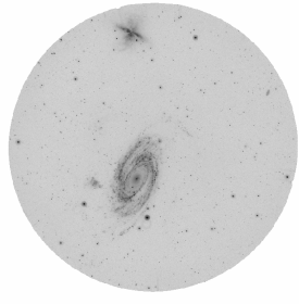
Fig. 1 : GALEX NUV image of the M81 and M82 galaxies with the field of view overlaid.

However, building a mosaic involves more information than just pure astrometry. Even in well planned space-based surveys, such as the all-sky survey runs by the Galactic Evolution Explorer (GALEX-AIS), exposure times are not exactly the same, nor background levels. Thus, building a scientifically useful mosaic requires to correct for background levels, as well as to define algorithms that include flux rebinning when geometric re-projection is applied.

Aladin is an interactive software developed and maintained by the Strasbourg astronomical Data Center (CDS) and used extensively by the astronomical community to visualize images coming from different sources and surveys. The astronomical image mosaic engine developed at Caltech/JPL for its space missions is Montage, a toolkit for assembling FITS images into custom mosaics. However, it does not suit well for mosaicking GALEX images. The field of view of GALEX is circular (see Figure 1). The FITS file contains zeros outside the field of view. The Montage task mFixNan can be used to convert a range of supplied values into NaNs. One may be tempted to use this task to convert every pixel with a value equal or lower than zero into a NaN. However, this approach causes several problems when the resulting images with NaN values are mosaicked with Montage. The exposed field of the image may also contain pixels with a value of zero and they would not be treated by Montage.

The next UV mission to be flown is the World Space Observatory - Ultraviolet (WSO-UV) (shustov3). WSO-UV is a 170 cm primary telescope equipped with instrumentation for imaging and spectroscopy in the ultraviolet (UV) range, from 115 to 320 nm. ISSIS is the imaging instrument on board WSO-UV and it will be equipped with Micro-Channel-Plate (MCP) detectors, as the GALEX mission, which have very low read-out noise (to detect weak extended structures) but that can be damaged by high count rates (issis0; issis). The ISSIS team will extensively use the GALEX database to select interstellar regions for future research and to define avoidance regions. For this purpose, we require large UV maps of the sky where interstellar features extending over several degrees in the sky (see Figure  2) can be properly studied. Given the limitations of the Montage software, we developed our own software, MOSAIX, that we make available (subsection 3.3.3) to the scientific community.

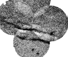
Fig. 2 : GALEX FUV image of an Interstellar Medium filament covering more than 2 degrees in the sky. This mosaic was generated with Aladin.

The paper is organized as follows. In Section 2 a brief outline on GALEX data is provided. The algorithm is described in Section 3 and the tests we have run are detailed in Section 4. Further useful information and implementation details can be found in Section 3.3. Conclusions and future work are summarized in Section 5.

2 About GALEX images

GALEX performed an all-sky survey in the far ultraviolet (FUV) and near ultraviolet (NUV) bands (galex1). Releases from the mission include the archive stored in the NASA Mikulski Archive for Space Telescopes (MAST) as well as high level science products like the point source catalogue (bianchi). Our work uses images obtained by GALEX in the far ultraviolet, 135-175 nm, or FUV band and in the near ultraviolet, 175-280 nm, or NUV band. The current release of the GALEX archive contains data products from the mission pipeline. Most of them are FITS files, both tables and images. The archive contains flux-calibrated images in the NUV and FUV bands, in photons per second per pixel, as well as background-substracted intensity maps and count maps (photons/pixel) in both NUV and FUV. For this work, intensity maps without background subtraction were used because it is a better choice when looking for extended weak structures. However, for high sensitivity applications we recommend the user to substract the sky background prior to mosaicking. Note that the GALEX mission provides background substracted images among its standard output products.

The information contained in the FITS header is used to compute the projection elements for building the mosaic. NAXIS1 and NAXIS2 are the sizes (in pixels) of the data for the horizontal and vertical axis, respectively. The GALEX mission database provides $3840\times 3840$ pixels images. The RA_CENT and DEC_CENT values are the right ascension and declination of the target point and they correspond to the central pixel coordinates ($1920.5,1920.5$) that are given by the parameters CRPIX1 and CRPIX2. The increase step for each axis is given by CDELT1 and CDELT2 and it is always $=4.1667\times 10^{-4}$ degrees/pixel (equivalent to 1.6 degrees / 3840 pixels). The angle between the North and the second axis (CROTA2) is always zero for the GALEX images we are using in this work. With this information read from the header the coordinates of every point on the image can be computed. The matrix of pixels representing the image has only one channel with a given view size of $1.28$ degrees (in FUV) or $1.24$ degrees (NUV).

3 Merging algorithm

GALEX images are generated in gnomonic projection (galex1), i.e. the celestial sphere is projected on the plane of the sky considered to be tangent to the sphere in the center of the field (green). Projection effects are not considered at this stage of the software development. Distortion effects are negligible for the GALEX field of view. For the correct image alignment both the angular distance and the rotation angle between the images must be known. We first present how two images are assembled together (Section 3.1) and then we generalize it (Section 3.2) for more than two images.

3.1 Two images

The alignment of the reference system is made in two steps: displacement (3.1.1) to match the center of the two images and then, rotation (3.1.2). The generic procedure can be summarized as follows: First, we build the required canvas (in a matrix grid) for the mosaic and then the first image is mapped to it without any motion or rotation. We name this first image the baseline image. Finally, the inset image is added to the canvas after moving and rotating it to completely match the baseline image in overlapping portions.

3.1.1 Translation

Let ($C_{x}$,$C_{y}$) be the center of the baseline image in the new canvas and, associated to this reference pixel, the coordinates of the baseline image must be read from the header. Let ($\alpha_{0}$,$\delta_{0}$) $\in\mathbb{R}$ be the coordinates of this point which are the right ascension ($\alpha_{0}$) and declination ($\delta_{0}$) respectively. Let ($\alpha,\delta$) $\in\mathbb{R}$ be the center coordinates of the inset image.

The distances $\Delta x$ and $\Delta y$ (in pixels) between the center of the two images are computed (gnomonic) as,

$$A = \cos(\delta)\times\cos(\alpha-\alpha_{0})$$ (1)

$$F = s\times\frac{\left(180/\pi\right)}{\sin(\delta_{0})\times\sin(\delta)}+(A\times\cos(\delta_{0}))$$ (2)

$$\Delta y = -F\times(\cos(\delta_{0})\times\sin(\delta))-(A\times\sin(\delta_{0}))$$ (3)

$$\Delta x = -F\times\cos(\delta)\times\sin(\alpha-\alpha_{0})$$ (4)

being $s$ the pixel scale. The variables $\Delta x$ and $\Delta y$ fit the offset between the two images but they must be integers, thus we use the $round$ function to find the nearest integer:

$$X = round(C_{x}+\Delta x)$$

$$Y = round(C_{y}+\Delta y)$$ (5)

3.1.2 Rotation

In Figure 3 the orientation of the images in the plane of the sky is shown. Both the center of the baseline image ($\alpha_{0},\delta_{0}$) and the center of the inset image ($\alpha,\delta$) are marked.

If the position angle in the FITS file header is zero no rotation needs to be applied and the y-axis of the digital image, the vertical line in the figure, is aligned with the polar direction. As a result, the angle between the two images can be computed as:

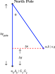
Fig. 3 : Sketch of the relative position of two GALEX images projected on the sky tangent plane.

$$\theta = \arctan\left(\frac{\Delta x}{\Delta y_{pole}-\Delta y}\right)$$ (6)

3.2 More than two images

When only two images are processed the coordinates of one of them can be used as a reference for the output mosaic. In multiple merging, the point located at the middle of the whole set of images is associated with the center pixel of the new FITS image canvas. This point will be the baseline point and all the merging images will be shifted and rotated around it for being inserted into the canvas.

3.2.1 Computing the canvas size

From a set of FITS images with central coordinates ($\alpha_{i},\delta_{i}$), the resulting canvas size is computed in four steps:

1. The first size estimate (in degrees) is computed from the centers of the images:

   $$\Delta\alpha = \max(\alpha_{i})-\min(\alpha_{i})$$

   $$\Delta\delta = \max(\delta_{i})-\min(\delta_{i})$$ (7)

2. The pixel scale ($s$) is applied to convert angular distances into pixels.

3. Then, a frame is added to the canvas. If each single image has $N$ pixels per side, the canvas size ($W\times H$) will be:

   $$H = N+(\Delta\alpha\times s)$$

   $$W = N+(\Delta\delta\times s)$$ (8)

4. Finally, the canvas size is made a little bit larger because rotation effects may prevent that an image is properly inserted. Note that the worse case is an image to be placed in the corner of the canvas that must be rotated by 45 degrees. A pixel frame of around 795 pixels would be needed in this case.

We must point out that the possibility to perform pixel resampling is not offered in this first version of the software. That is, the final canvas pixel size is the same as the original GALEX images (1.5 arcsec/pixel).

3.2.2 Center (baseline) point

In a multiple image merging task, nearly all the pictures will be rotated. Our approach fixes a central reference point in the middle of the image with its space coordinates rightly defined ($\alpha_{c},\delta_{c}$). This is the midpoint between maximum and minimum coordinates and it is associated to the central pixel ($W/2$,$H/2$) of the canvas:

$$\alpha_{c} = \min(\alpha_{i})+\frac{\Delta\alpha}{2}$$

$$\delta_{c} = \min(\delta_{i})+\frac{\Delta\delta}{2}$$ (9)

3.2.3 Algorithm

In Section 3.1 we described the simple case when only two images are being aligned. For more than two images, after calculating the canvas size ($W\times H$) and its central point ($\alpha_{c},\delta_{c}$), the algorithm follows the next steps:

1. For each FITS image:

   • Computing the pixel distance between center of the $i$-th image and the coordinates ($\alpha_{c}$,$\delta_{c}$) of the central pixel ($W/2$,$H/2$) of the canvas, by using the equations shown in Section 3.1.1.

   • Insert the image on the appropriate place.

   • Make the rotation with Equation 6 for completing the alignment.

2. Write the data matrix on a FITS file, adding the correspondence between the central ($\alpha_{c}$,$\delta_{c}$) coordinates and the central ($W/2$,$H/2$) pixel position in its header, and write the scale factor and other information in the header.

3.3 Software details

3.3.1 Pixel average

The simple way for computing the average intensity of each pixel (in MatLab™) requires the use of the NaN values for the surrounding black area of the image. Actually, if GALEX images are processed with Montage, this NaN set up must be done by the user (with other software) or some strip effects could appear on the overlapping areas.

A multi-layer matrix where these surrounding non-signal pixels have NaN values lets MatLab™  use of nansum function to add only data values. With this method, each layer will store only an image matrix at the first step of the process. When all the images are placed in their correct position the average of the intensity is possible along the third dimension of the cube. Figure 4 shows an example with two images correctly aligned. Each image is placed in its own layer. Computing the resulting matrix in this case requires the before mentioned averaging.

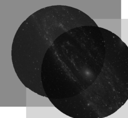
Fig. 4 : Two merging FITS on one image per layer cube. Final average must be computed along the third dimension (perpendicular to the paper). The NaN frame around the image is shown in gray colors.

With the purpose of an effective use of the system resources (particularly the computer memory), a single-layer matrix can be used if the sum and average of each new incorporated image are made inside a bounded sub-matrix equivalent to the size of the new added image.

3.3.2 Rotation

Image rotation requires some operations with pixel values that can create distortion because the presence of noise in the signal data. The resulting matrix will have in each pixel a linear combination of original values. Our recommendation for completing the rotation process (in MatLab™) involves the use of the imrotate function applying the nearest neighbour modality so that a loss-less interpolation be reached. This option searches, among the original values, the most similar numbers to the estimated output.

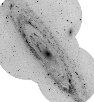
Fig. 5 : Final reconstruction of M31 galaxy from several FITS files.

3.3.3 Availability

MOSAIX is a set of MatLab™ scripts to build big mosaics from GALEX images. The original scripts are available at the odin.estad.ucm.es/mosaix web site. The scripts are prepared for a friendly use with three parameters: (1) the folder of the FITS files (2) the name of the output file and (3) a boolean flag for intermediate plots. Get your mosaics typing in the MatLab™ prompt the next command:

totalmerging(’folder/’,’test.fits’,0)
 

4 Tests

4.1 Image quality

The mosaicking process involves interpolation for rotation, averages of overlapping areas and numerical rounding. Comparing the result with the original data is the only way to check how much the data was modified, mainly when the aim of this task is to do other kind of analysis with the final image.

Seven FUV images from GALEX were used to generate our first mosaic, shown in Figure 5. For a reference comparison, the Montage tool was used too with the same set of images. Figure 6 shows a $1000\times 1000$ pixels section of the mosaic where the quality tests were applied.

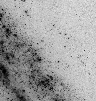
Fig. 6 : Section of the final image where an overlapped area is included. Several subimages of this region have been processed in the image quality tests. The same section was taken from MOSAIX as well as from Montage, for testing the similarity with the original image (without overlapping).

Two quality measures were used comparing the mosaic data with the original data. First, the classical Peak Signal-to-Nosie Ratio (PSNR) defined as $PSNR=10\log_{10}(MAX^{2}/MSE)$, where $MAX$ is the maximum possible value of the signal and $MSE$ is the mean square error between the original signal and the mosaic result. Second, the Structural Similarity (SSIM) index which measures the similarity between two images and is defined as follows:

$$\hbox{SSIM}(x,y)=\frac{(2\mu_{x}\mu_{y}+c_{1})(2\sigma_{xy}+c_{2})}{(\mu_{x}^{2}+\mu_{y}^{2}+c_{1})(\sigma_{x}^{2}+\sigma_{y}^{2}+c_{2})}$$ (10)

being $\mu_{x}$ the average of the first image (called $x$), $\mu_{y}$ the average of the second image (called $y$), $\sigma_{x}^{2}$ the variance of $x$, $\sigma_{y}^{2}$ the variance of $y$ and $\sigma_{xy}$ the covariance of $x$ and $y$. $c_{1}=(k_{1}L)^{2}$ and $c_{2}=(k_{2}L)^{2}$ are two variables to stabilize the division with weak denominator. The parameter $L$ is the dynamic range of the pixel-values, and $k_{1}=0.01$ and $k_{2}=0.03$ by default. The performance of this measure has been shown recently by ssim. Figure 7 shows the results for several image sizes. In both cases (SSIM and PSNR) the differences are negligible, that is both programs produce final images that are very similar to the original ones in the overlapped regions.

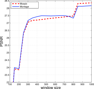
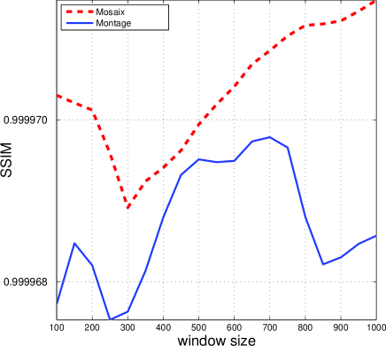
Fig. 7 : Tests of comparison between original images and merged mosaics. On the top, PSNR measure is shown. On the bottom, the SSIM is shown in logarithmic axis. Both of them show the results for different window sizes of the image. The values are so close to the maximum value (1) that it was needed to zoom into the vertical axis.

4.2 Execution time

Montage software was developed to be able to work in several CPUs. However, for the common user the time to compute the total mosaic (in a single machine) is the most important factor to be considered. The timing tests were made on a multicore workstation with four cores for eight running threads Intel(R) Core™i7 CPU 920 2.67 GHz and 6 Gb of RAM memory. Five overlapped images (increasing the mosaic field of view) were processed with the Montage software. The same operations were processed with our scripts. To get the computing time the bash script time command was used for Montage and the cputime MatLab™ function for our scripts. Figure 8 shows that, as expected, the execution time increases with the size of the mosaic. However, our scripts show an improvement compared with Montage.

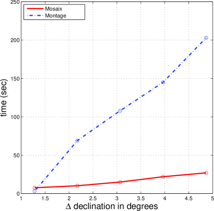
Fig. 8 : Test of processing time. Several sized mosaics were processed with Montage software and our scripts. Vertical axis shows the time elapsed in each case.

5 Some conclusions and future work

This paper summarises the main characteristics of Mosaix, the tool developed by our team for mosaicking GALEX mission images. Our software accomplishes the standards of Montage in terms of overlapping quality and re-projection and guarantees no loss of information in the overlapping regions. As a specific tool for GALEX, our software is optimized to work with images from this mission. The user needs to provide only the original images from GALEX and run the programme. Previous operations with the GALEX images are not needed, contrarily to Montage. Velocity tests demonstrate our software is faster than Montage in single processor usage (we note that Montage can be run also in parallel mode). There are several improvements suitable to be incorporated in future versions such as the possibility of user-specified regridding or the generalization to images from other missions. This initial version of our software is distributed for MatLab™. Subsequent versions for IDL will be provided in the future.

Acknowledgements

Thanks to Dr. Jason Dieter Fiege, writing resulting matrix in a FITS file is easy. With his mfits library we can fit coordinates and other header settings. We would like to thank the anonymous referee for many useful comments that improved this paper. We acknowledge financial support from Ministerio de Economía y Competitividad of Spain through grant AYA2011-29754-C03-01