Numerical modelling of the lobes of radio galaxies in cluster environments II: Magnetic field configuration and observability

Abstract

We describe three-dimensional magnetohydrodynamical modelling of powerful radio galaxies in realistic poor cluster environments. This modelling extends our earlier work on the hydrodynamics of radio galaxies as a function of their cluster environment to consider the magnetic field configuration in the lobes and its observational consequences, using a realistic model for the magnetic field in the intracluster medium, very high density contrast in the lobes and high numerical resolution. We confirm, now with a realistic magnetic field model, that lobes have characteristic trajectories in the radio power/linear size diagram which depend strongly on their environment. We investigate the detailed evolution of polarized emission, showing that the lobes evolve from the initially ordered field configuration imposed by our boundary conditions to one in which the longitudinal field comes to dominate. We obtain simulated observations of polarization whose properties are quantitatively consistent with observations. The highly spatially intermittent magnetic field also reproduces the observation that inverse-Compton emission from lobes is much smoother than synchrotron. Our simulations allow us to study the depolarizing effect of the external medium on the lobes, and so to demonstrate that Faraday depolarization from environments of the type we consider can reproduce the integrated fractional polarization properties of large samples and the observed preferential depolarization of the receding lobe.

1 Introduction

Numerical modelling of powerful radio-loud active galaxies is an essential tool towards developing a full understanding of the evolution of these sources and their interaction with their environment. On the large scales on which these sources are best observed (physical scales of hundreds of kpc to Mpc) observations of the best-understood class, powerful Fanaroff & Riley (1974) class II (FRII) sources, show very complex, disparate structures in the radio (e.g. Black et al., 1992; Bridle et al., 1994; Leahy et al., 1997) and also occupy a wide range of hot gas environments, often also showing complex structure (Hardcastle et al., 2001; Wilson et al., 2006; Kraft et al., 2006, 2007; Belsole et al., 2007; Chon et al., 2012; Ineson et al., 2013). Numerical modelling can now routinely deal with reasonable approximations to the sort of large-scale hot-gas environments that radio sources inhabit (Reynolds et al., 2002; Basson & Alexander, 2003; Zanni et al., 2003; Krause, 2005; Heinz et al., 2006; Mendygral et al., 2012) as well as to smaller-scale galactic environments (Gaibler et al., 2011; Wagner & Bicknell, 2011; Gaibler et al., 2012; Wagner et al., 2012; Cielo et al., 2014) while the physics of the radio lobes can be made closer to what we know to be realistic by considering magnetohydrodynamic (MHD) rather than purely hydrodynamic (HD) modelling, and by considering electron acceleration and loss processes (Clarke et al., 1989; Matthews & Scheuer, 1990; Tregillis et al., 2001, 2004; Gaibler et al., 2009; O’Neill & Jones, 2010; Mignone et al., 2010; Huarte-Espinosa et al., 2011a). While numerical models never include all of the physics that is necessary to describe a real radio galaxy, and are often limited by numerical resolution, we may be converging on approximations that are good enough to allow us to learn about the radio galaxy population, rather than individual pieces of radio galaxy physics, by comparison with simulations.

In a previous paper (Hardcastle & Krause, 2013, hereafter Paper I) we described two-dimensional, purely hydrodynamical models of the radio-emitting lobes driven into groups and clusters of galaxies by powerful double radio galaxies. Our objective in that paper was to establish the general effect of such sources on the intracluster or intragroup medium by studying the effect of varying (realistic) parameters describing the medium on the radio source, and at the same time to establish how well the time evolution of basic parameters of the radio source (length, volume, synchrotron luminosity) matched observations on the one hand and analytical models such as those of Kaiser & Alexander (1997) on the other. Restricting ourselves primarily to two-dimensional, axisymmetric modelling gave us sufficient spatial resolution to model the jets from the kpc-scale on which initially conical jets become collimated out to the scale of a few hundred kpc on which large double radio sources are seen. We established a number of important results, including (i) clear evidence for departures from self-similarity of the lobes and for the removal of the lobes from the centre of the cluster by buoyancy once the inner parts of the lobes come into pressure balance with the external environment, (ii) evidence that tracks in the power-linear size diagram for powerful radio sources are strongly influenced by their environment, and (iii) evidence that a roughly constant fraction, close to unity, of the energy stored in the lobes goes into work done on the external medium.

In the present paper we apply the same approach to three-dimensional, magnetohydrodynamical (MHD) simulations of radio galaxies. Our reasons for this are threefold:

1. It is important to check whether the conclusions of Paper I are valid in the case of a non-axisymmetric, magnetized outflow; earlier work (e.g. that of O’Neill et al. (2005) and Gaibler et al. 2009 for MHD) supports this, but the best way of testing it is to run more realistic simulations in the same environments as those of Paper I.

2. Magnetic fields, in particular, are essential for realistic synchrotron visualization, and allow us to consider polarized emission from our simulated radio sources for the first time. This allows comparison with the work of Huarte-Espinosa et al. (2011a, b), repeating their pioneering work in this area at higher numerical resolution and comparing with observations.

3. Incorporating three-dimensional structures and magnetic fields is a further step on the way towards models of FRII radio galaxies that contain all the physics necessary to compare with observations. Here, we aim to establish the magnetic field configuration in radio lobes.

Section 2 describes the setup of our new simulations and Section 2 our results. The key results and the extent to which we believe them to be relevant to real objects are summarized in Section 4.

2 The simulation setup

Our modelling in this paper, as in Paper I, uses the MHD implementation in the freely available code PLUTO, version 4.0, described by Mignone et al. (2007). In particular, we used the hlld solver with the divergence cleaning algorithm to enforce $\nabla\cdot{\mathbf{B}}=0$ (the eight-wave method tended to wash out fine magnetic structure in the simulated lobes while we were unable to use constrained transport with our choice of internal boundary condition). We used dimensionally unsplit second-order Runge-Kutta time stepping with a Courant-Friedrichs-Lewy (CFL) number of 0.3.

Since in this paper we are attempting to carry out fully three-dimensional, MHD calculations, we cannot use the very high resolution of Paper I, which was intended to allow us to generate self-consistent, collimated jets from an initially biconical outflow. Time and physical memory constraints restrict us to a fiducial simulation using a $400\times 400\times 400$-element volume. We do not use the adaptive mesh refinement capability of PLUTO in order to preserve the small-scale magnetic field fluctuations in the jet’s ambient medium (see below for details). As a direct consequence of this grid setup, we cannot inject a conical jet which will self-collimate on the appropriate physical scale – instead we take a similar setup to that used by Huarte-Espinosa et al. (2011a) (hereafter HE11), and inject a bipolar jet using an internal boundary condition which is a cylinder of radius $r_{j}$ and length $l_{j}$ along the $x$-axis, internal to which we have $\rho=\rho_{j}$, $v_{x}=\pm{\cal M}_{j}c_{s}$, $v_{y}=v_{z}=0$ and $p=T_{j}\rho_{j}$. The injected field structure is purely toroidal with $|{\mathbf{B}}|=B_{j}$. A conserved tracer quantity is injected with the jets, taking the value 1.0 at injection and 0 everywhere else in the grid at the start of the simulation. Both the injected jets and the ambient medium are treated as ideal gases with $\gamma=\frac{5}{3}$. The outer boundary conditions are periodic.

Table 1: Key initial simulation parameters in physical units

Fluid	Quantity	Value	Units	Location
Jet	Kinetic power	$10^{38}$	W	(One-sided)
	Density	3.75	m-3	Injected
	Speed	$7.3\times 10^{4}$	km s-1	Injected
	Temperature	8	MeV	Injected
	Radius	4.2	kpc	Injected
	External Mach number	100		Injected
	Internal Mach number	1.6		Injected
	Magnetic field strength	0.15	nT	Injected, fiducial
	Plasma $\beta$	400		Injected
Cluster	Density	$3\times 10^{4}$	m-3	Central
	Temperature	2.0	keV	Everywhere
	Sound speed	730	km s-1	Everywhere
	RMS field strength	0.7	nT	Central
	Plasma $\beta$	40		Everywhere

For continuity with Paper I, we take the environments of the radio sources to be rich groups or clusters, with a density profile given by

$$n=n_{0}\left[1+\left(\frac{r}{r_{\rm c}}\right)^{2}\right]^{-3\beta/2}$$ (1)

The core radius and value of $\beta$ are variable, as described below. PLUTO simulations are run using scalable simulation units, but in our case we wish to represent a specific physical situation, so, to match Paper I, we take the simulation unit length to be $L=2.1$ kpc, the unit temperature to be $kT=2$ keV, and the central density to be $n_{0}=3\times 10^{4}$ m^-3. As in Paper I $c_{s}=730$ km s^-1, meaning that the simulation time unit is $\tau=L/c_{s}=2.9\times 10^{6}$ years. In terms of volume, we go out to a maximum radius of $\pm 150$ simulation units ($\pm 310$ kpc), again as in Paper I, so that the volume elements of our fiducial simulation are 0.75 simulation units, or 1.6 kpc on a side.

The assumptions we make about the environment then to some extent control the properties of the jet that is injected. We must put in by hand the condition that was automatically satisfied by our self-collimating jets in Paper I, namely that $p_{j}\approx p_{0}$, where $p_{0}$ is the central pressure, or $p_{j}\approx 1$ in simulation units. Thus if the jet is light, with $\rho_{j}\ll 1$ in simulation units, then necessarily $T_{j}\approx 1/\rho_{j}$; we follow Paper I, Gaibler et al. (2009) and ultimately Krause (2003) in our assumption that a very light jet is required to make realistic lobes. If we require that the initial jet advance be supersonic, then in addition ${\cal M}^{2}_{j}\rho_{j}>1$. Note that marginally satisfying this constraint, with ${\cal M}^{2}_{j}\rho_{j}=1$, leads to $T\approx{\cal M}_{j}^{2}$, i.e. to a jet which is trans-sonic in terms of its internal sound speed at injection. However, since the nominally injected jet power can be written (in simulation units, and writing in terms of the enthalpy since the jet is hot, we have

$$Q=\pi r_{j}^{2}{\cal M}_{j}\left(\frac{1}{2}{\cal M}_{j}^{2}\rho_{j}+\frac{5}{2}T_{j}\rho_{j}+\frac{B^{2}}{2}\right)$$ (2)

we see that the jet that supplies minimal power for a given $r_{j}$ while still obeying the constraint ${\cal M}^{2}_{j}\rho_{j}>1$ is precisely this type of trans-sonic, hot jet, and in this limit the energy supply is predominantly in the form of the enthalpy of the jet material rather than the kinetic energy density (assuming that the term involving the magnetic energy density may be neglected). We can change the balance between kinetic and thermal energy content only by increasing the jet Mach number such that ${\cal M}_{j}^{2}\gg 1/\rho_{j}$.

For our simulation setup, we have a further constraint which is that $r_{j}$ cannot be made so small that it is not reasonably well resolved by the simulations (i.e. smaller than a few simulation cells). We adopt ${\cal M}=100$, and then choose $\rho_{j}=1.25\times 10^{-4}$, $T=4000$ and $r_{j}=2.0$ in simulation units: this gives a (one-sided) jet power in physical units of $10^{38}$ W, consistent with our previous work (see Table 1 for the full physical properties of the jet). The external Mach number of 100 (corresponding to a speed around $0.24c$ in physical units) is the largest that can reasonably be used without needing to take account of the effects of special relativity, and the jet temperature corresponds to relativistic particle energies for electrons, so that we are at least close to the regime thought to be occupied by real radio galaxies. However, it is important to note that the jet is slower than, and very likely has a lower internal Mach number than, the jets in real FRII radio galaxies; a consequence of this is likely to be weaker internal shocks and a consequent suppression of ‘hotspot’ structure. We comment further on the relationship between our assumed source properties and real FRII sources in Section 4.1.

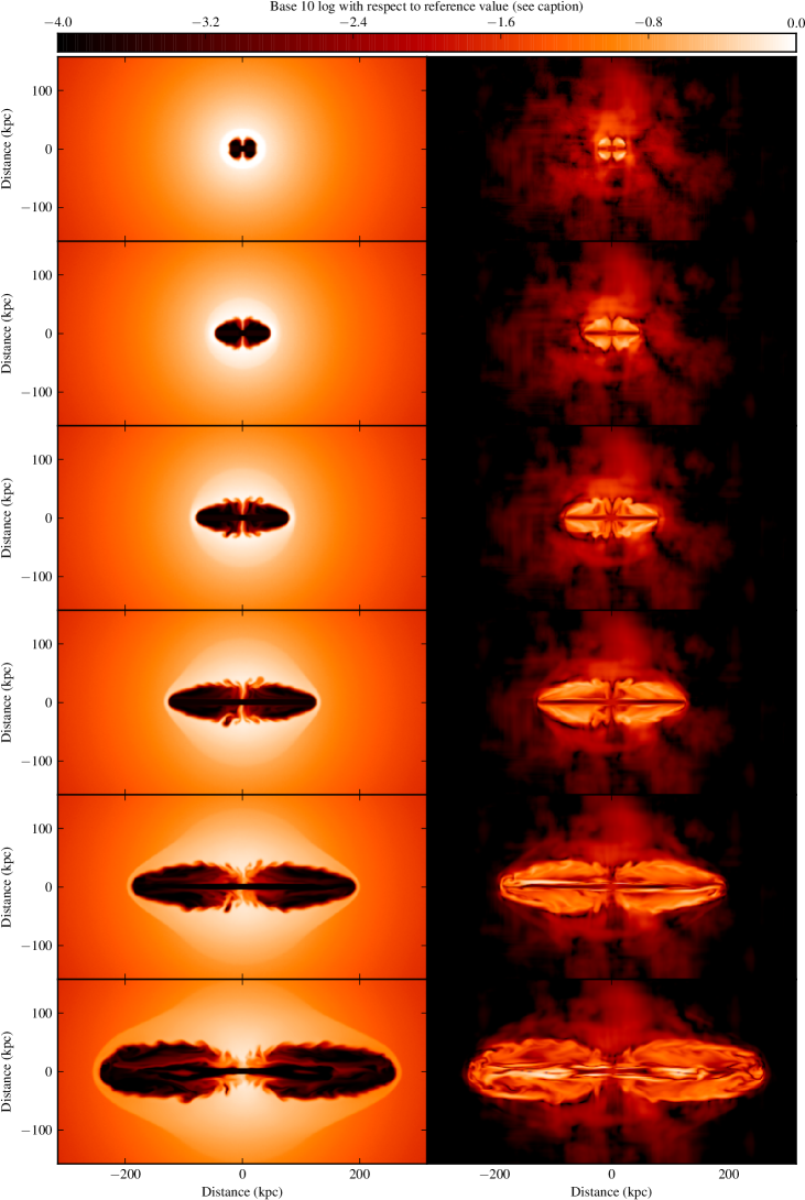
Figure 1: Particle density (left) and magnetic field energy density (right) slices in the central $xy$ plane for B75-30 at simulation times $t=30,60\dots 180$ Myr as a function of position. Colours show the base-10 logarithm of both quantities relative to the cluster-central value at $t=0$ (for density) and a reference value corresponding to $B=1.8$ nT (for field energy density).

We adopt a fiducial value of $B_{j}$ of 0.05 (simulation units) which corresponds to about 0.15 nT in physical units. This input number constrains the normalization of the field in the lobes, as we will discuss later. More importantly, we follow HE and set the field in the ambient medium to be a Gaussian random field whose energy density scales with pressure, with a peak field strength in the centre of the medium of 0.7 nT (this is consistent with field strength measurements in real groups and clusters of galaxies, see e.g. Guidetti et al. 2012). We put in a power spectrum of the magnetic field strength corresponding to Kolmogorov turbulence in the manner described by Murgia et al. (2004) and Hardcastle (2013), cutting the spectrum off below size scales of $\sim 3$ pixels to avoid injecting high-spatial-frequency structure into the simulations (this would immediately be damped out by numerical effects in any case, and removing it gives a more useful baseline simulation at $t=0$). We emphasise that the scaling of the magnetic energy density with pressure ensures that little power is present in the spectrum of the magnetic field on scales larger than the core radius, though the unscaled power-law spectrum extends to structures with scales comparable to the half-size of the simulation volume. In this way we attempt to model a realistic magnetic environment for the jet.

We run three sets of simulations to investigate the jet behaviour as a function of different parameters:

1. A set of 9 simulations varying the parameters of the environment, with $\beta=0.55$, 0.75 and 0.90 and $r_{c}=20$, 30 and 40 simulation units (roughly 40, 60 and 80 kpc). This is similar to the range studied in Paper I except that in this paper we do not carry out simulations with $\beta=0.35$, which we consider rather too flat to be realistic.

2. A set of 4 simulations varying the input magnetic field strength, all with $\beta=0.75$ and $r_{c}=30$. The magnetic field strength injected in the jet controls the field strength found in the lobes. In simulation units these have $B_{j}=0.01$, 0.02, 0.05 and 0.1.

3. A set of two simulations with $\beta=0.75$, $r_{c}=30$, $B_{j}=0.05$, one of which has a significantly higher resolution (a $600\times 300\times 300$ simulation covering the same physical volume in the $x$ direction, i.e. with elements a factor 1.5 smaller in all dimensions). This allows us to investigate any resolution effects in our results on e.g. polarization. Because of the smaller physical size of the simulations in the $y$ and $z$ directions, the high-resolution simulation does not capture the full shock size at late times, and so needs to be used with caution when the external medium is considered. These two simulations have the same initial conditions for the external medium so that effects of different environments can be distinguished from resolution effects.

4. One simulation with $\beta=0.75$, $r_{c}=30$ with standard resolution but a $664\times 300\times 300$ box, thus allowing the lobes to extend to $\pm 250$ simulation units at the cost of no longer being able to track the shocked gas accurately. This run is only used where required to test convergence of lobe properties that evolve with length.

In what follows we assign each simulation a code of the form Bxx-yy… for brevity; these codes are used to identify results from individual simulations in the plots in the following section. The codes and the properties of the simulations they map onto are listed in Table 2. As the B75-30 simulation (and its high-resolution counterpart B75-30-HR) have non-extreme environmental properties they are generally used as illustrations when specific simulations are required in what follows: their properties can be taken as representative unless otherwise stated.

Table 2: Parameters of the ambient density profile, $\beta$ and $r_{c}$ as in eq. 1 explored in this paper, with other specifics of the individual simulations. Cluster core radii are given in simulation units, equal to 2.1 kpc.

Code	$\beta$	$r_{c}$	Other notes
		(sim. units)
B55-20	0.55	20
B55-30	0.55	30
B55-40	0.55	40
B75-20	0.75	20
B75-30	0.75	30
B75-40	0.75	40
B90-20	0.90	20
B90-30	0.90	30
B90-40	0.90	40
B75-30-HM	0.75	30	$2\times$ normal jet field
B75-30-LM	0.75	30	$0.4\times$ normal jet field
B75-30-VLM	0.75	30	$0.2\times$ normal jet field
B75-30-HR	0.75	30	$1.5\times$ normal resolution
B75-30-LONG	0.75	30	Long, thin grid

All our production runs were carried out using the STRI cluster of the University of Hertfordshire, using between 128 and 256 Xeon-based cores, typically for about 24-48 hours per run, terminating the run when the shocked region reaches the grid boundary. (Simulations other than B75-30-LONG therefore all extend to a total lobe length of around 300 kpc, though the amount of simulation time required to reach the edge varies widely.) PLUTO was configured to write out the complete state of the simulation every 1 simulation time unit (3 Myr) and these images of the simulation grid were used to compute derived quantities such as the dimensions of the lobe, the energy stored in the lobe and in the shocked region, and so forth. We use the conserved tracer quantity to define regions inside and outside of the lobes in the analysis that follows. For consistency with Paper I, we define a contiguous volume as being inside the lobes, which in this paper is the volume internal to a surface at which the tracer quantity is everywhere $>10^{-3}$. (We note that it is possible for the tracer to be $<10^{-3}$ inside this volume, e.g. if there is large-scale entrainment of thermal material, but this definition in practice appears to give a sensible lobe boundary, as did the equivalent definition in Paper I.) The results are insensitive to the tracer threshold chosen as long as it is not too high. We define the shocked region as being the region external to the lobe boundary with an outward radial velocity greater than 0.1 in simulation units. The volume outside the shocked region is not considered in any calculation of the energetics. As in Paper I, calculation of energies for the shocked region take as their zero point at any given time $t$ the energy stored within the boundary of the shock at time $t$ in the image from $t=0$, so that we correct for the pre-existing internal energy of the environment.

In postprocessing we retain the ability to distinguish between the two lobes of the radio galaxy (the magnitude of differences between the two gives an estimate of the effects of the slightly different initial conditions on the two sides of the source) but in most plots presented below the quantities for the two lobes are summed or averaged, as appropriate, so as to give a single curve for each run. In particular, the reader should note that the lobe length, used in many of the plots below, is actually the mean of the lengths of the two lobes.

3 Results

In this section and throughout the remainder of the paper all results are presented converted to physical units, except where otherwise noted, in order to facilitate comparison with observations.

3.1 General simulation behaviour

Fig. 1 shows density and magnetic field energy density slices through the central $xy$ plane of the B75-30 simulation run, illustrating the broad features of the simulations’ behaviour. Qualitatively we see very similar behaviour to what was observed in Paper I in many respects, as expected since the objects we are simulating and their environments should be very similar. Here we focus on the important differences between the two sets of simulations.

• The expansion in the new simulations is slower at early times – this is because lobe formation is immediate in the new simulations as a result of the pre-heating of the jet material. The small aspect ratio of the lobes at early times in the new simulations (e.g. top panel of Fig. 1) is probably not realistic, however.

• The gap between the lobes is present from the earliest times in the new simulations, as a consequence of the non-zero starting length of the jet – it does not emerge naturally from the simulations as in Paper I. However, its growth with time is qualitatively consistent with our earlier work.

• The shape of the shock driven into the external medium is different at all times – presumably as a consequence of the different lobe dynamics.

Another important difference is of course the presence of magnetic fields, as shown in the right-hand panel of Fig. 1. The input magnetic field strength is chosen so as to mean that the magnetic field is globally dynamically unimportant, though locally that may not be the case; for example, the field is higher at the lobe edges and may provide non-negligible tension there. The global picture is illustrated in Fig. 2, which shows the total energy stored in magnetic field in the lobes compared to that stored in particle pressure as a function of lobe length. We see that the initial input field strength affects this, but that it is otherwise essentially independent of lobe length, environment, and numerical resolution. A mean ratio in energy density $U_{B}/U_{e}\sim 0.01$ (mean lobe plasma $\beta\approx 100$) is consistent with inverse-Compton energy estimates in real radio sources (Kataoka & Stawarz, 2005; Croston et al., 2005).

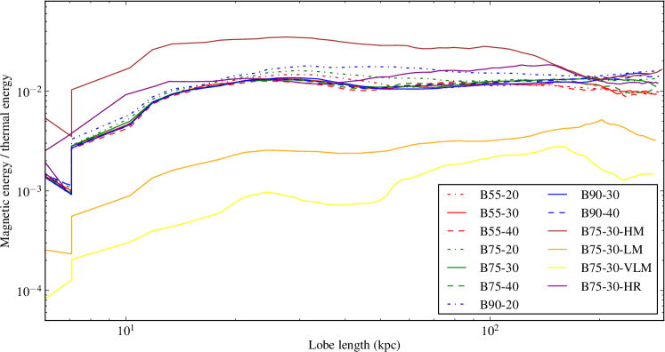
Figure 2: The ratio between the energy in field and that in particles integrated over the lobes, as a function of source length.

The simulations also give us the overall direction of the magnetic field in all times, which we may describe in terms of its toroidal, longitudinal and radial components relative to the jet axis (the $x$-axis). We find that there is always initially a strong toroidal component of the field, in the same sense as the injected toroidal jet field. At later times (earlier with weaker fields or at higher numerical resolutions), there are significant longitudinal and radial components as well, reflecting the dynamical effects of large-scale bulk motions inside the lobes (Fig. 3), and the longitudinal component becomes steadily more important as the lobes grow, possibly saturating around 60 per cent of the total magnetic field energy density as we see in the case of the weak-field runs B75-30-LM and B75-30-VLM. The evolution of this field component affects the polarization behaviour of the lobe, as we shall see in later sections.

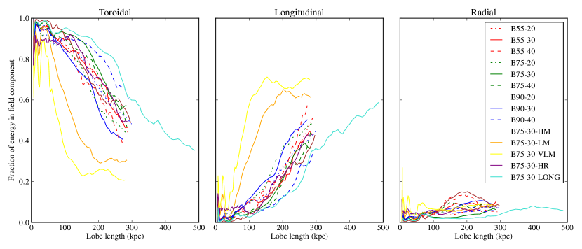
Figure 3: The fraction of magnetic energy in (left) toroidal, (middle) longitudinal and (right) radial components of the magnetic field. The long simulation B75-30-LONG is plotted here to show the long-term evolution of the field.

3.2 Lobe dynamics

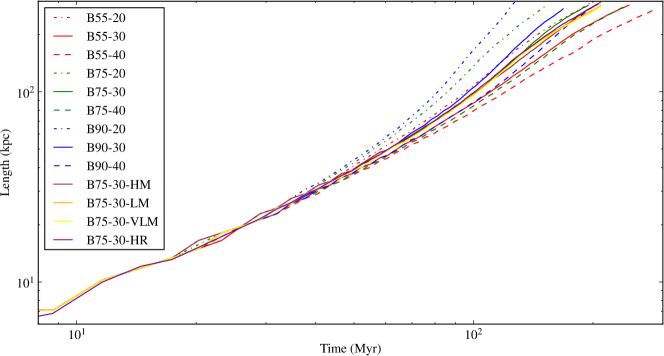
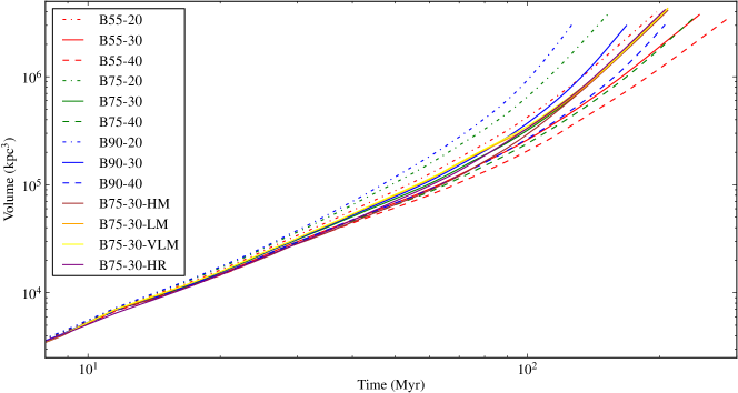
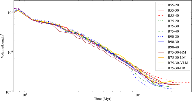
Figure 4: Growth of the lobes with simulation time. Top panel: mean lobe length $L$. Middle panel: mean lobe volume $V$. Bottom panel: $V/L^{3}$.

Quantitatively, the lobes show the expected approximately linear growth with time at early times; the lobe growth rate is limited by ram pressure balance at the jet head and so is roughly constant within $r<r_{c}$. Beyond the core radius of the environment, we see the expected steepening – the predicted slope (Kaiser & Alexander, 1997) is $5/(5-3\beta)$, and the three $\beta$ values clearly show the expected trends. The lobe volume scales with lobe length, but not in the sense expected from self-similarity: this is shown by the bottom panel of Fig. 4, which shows that the axial ratio varies by roughly an order of magnitude over the simulation time. The value plotted here would be constant if the lobes were self-similar. Departure from self-similarity is expected in real sources (Hardcastle & Worrall, 2000), as discussed at length in Paper I, and is a general feature of simulations (e.g. Krause 2005) so long as the source is not strongly overpressured at all times.

It is important to note at this point that the simulations with varying magnetic field and resolution do not deviate significantly from the fiducial simulation with the same environmental parameters. This is as expected, and shows that neither resolution nor magnetic field strength in the lobes affects the overall source dynamics.

3.3 Energetics of the lobe and environmental interaction

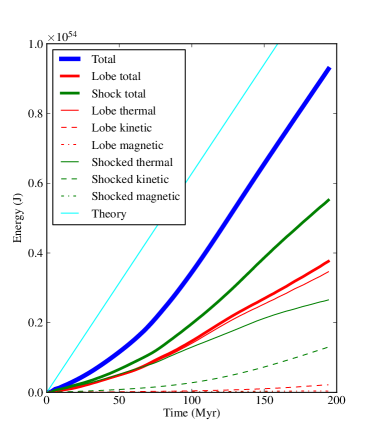
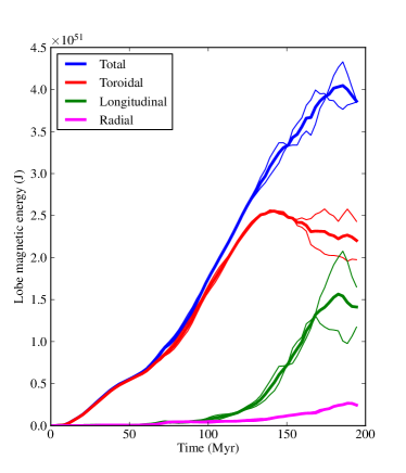
Figure 5: Left: energies in the lobe and shocked region as a function of simulation time for the B75-30 simulation. Also plotted (‘theory’) is the expected growth of the total if a constant energy flows in through the jet boundary condition. Potential energies are calculated in post-processing but not plotted here as their values are so small. Right: the same simulation, with the growth of lobe magnetic field energy and its three components in cylindrical co-ordinates as a function of simulation time. Thin lines on this plot show the curves for the two lobes separately (multiplied by 2) to provide a sense of the scatter imposed by ‘weather’ in the simulations.

The total thermal (particle), kinetic and magnetic energies in the lobes and shocked region can be plotted as a function of time to investigate the rate of energy injection into the system. An example is shown in Fig. 5 (left panel). We see that the energy input into the system falls below the expected value at all times: as with the simulations of Paper I, this arises because at early times the jet boundary condition does not couple well to the ambient medium, so that the jet flow on to the grid is partially suppressed. Once the lobes are well established the gradient of total energy is very comparable to expectations. The effect of this is to artificially lower the jet power at early times, at worst by of order a factor 2; this should be borne in mind when considering later results. However, at late times the discrepancy in total energy is only of order 25 per cent and can safely be ignored.

While the growth in the total energy in the system is linear, the growth in individual components need not be, as shown in Fig. 5 (right panel). The total energy in the magnetic field grows roughly as a constant fraction of the total energy in the system, but the longitudinal and toroidal components behave quite differently, reflecting the change in the field structure discussed above (Section 3.1). At about half-way through the run energy in toroidal field ceases to grow and even decreases slightly, with all subseqent increase being in the energy stored in the longitudinal and (to a much lesser extent) radial components.

We can also look at the ratio of energies stored in the shocked region and the lobe. One of the key results of Paper I was that this ratio was close to (typically a little larger than) unity, irrespective of the environment in which the source expanded. Fig. 6 shows this ratio as a function of lobe length. We see that in the current simulations this ratio is in the range 0.6-1.8, consistent with the previous work, but the scatter is a little larger than in Paper I and there are clear environmental dependences in the sense that the ratio is highest for higher $\beta$ and lower $r_{c}$, i.e. for lower-mass environments. It is not clear whether this difference with Paper I is because of the somewhat different lobe dynamics, as discussed above, or whether it arises from the absence of the naturally self-collimating jets of Paper I. However, the overall general agreement with the conclusion of Paper I is encouraging.

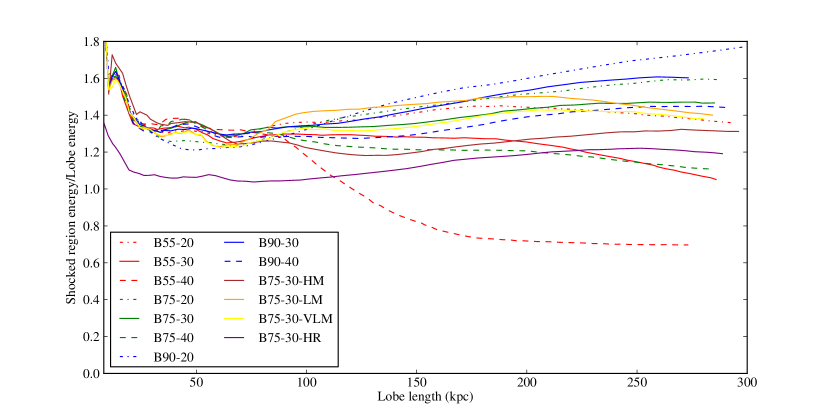
Figure 6: The radio of the energy in the shocked external medium and in the lobes as a function of lobe length.

3.4 Integrated radio emission

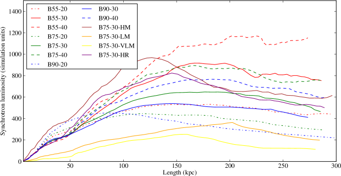
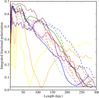
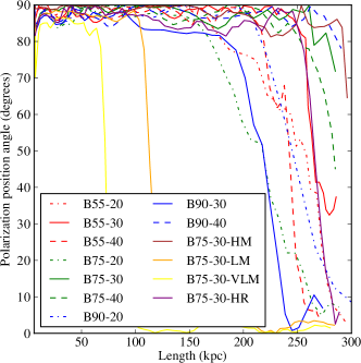
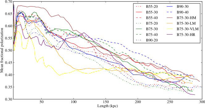
Figure 7: Synchrotron emissivity as a function of source length. Top: total intensity (luminosity). Middle: integrated fractional polarization and position angle (where zero means aligned with the jet axis). The horizontal black line shows the observed integrated fractional 1.4-GHz polarization for steep-spectrum sources of $\sim 2.5$ per cent (Tucci et al., 2004). Bottom: mean fractional polarization at full simulation resolution.

As in Paper I, we can calculate the integrated radio luminosity to see how this evolves with time or source length. Here we have the advantage that we actually know the magnetic field strength as a function of position, rather than simply assuming some constant deviation from local equipartition as in Paper I. (In fact, the idea that the energy density in the field traces that in the particles does not seem to be a particularly good assumption for these sources, as we will discuss later.) We therefore compute the Stokes $I$ (total intensity) synchrotron emissivity for the source making use of the local magnetic field vector, projecting along the $z$ axis for simplicity (in the absence of a fully tangled field, synchrotron emissivity is anisotropic, so we must choose direction from which to view the source). The Stokes $I$, $Q$ and $U$ emissivities, dropping physical constants, are then given by

$$j_{I} =p\left(B_{x}^{2}+B_{y}^{2}\right)^{\frac{1}{2}(\alpha-1)}(B_{x}^{2}+B_{y}^{2})$$ (3)

$$j_{Q} =\mu p\left(B_{x}^{2}+B_{y}^{2}\right)^{\frac{1}{2}(\alpha-1)}(B_{x}^{2}-B_{y}^{2})$$ (4)

$$j_{U} =\mu p\left(B_{x}^{2}+B_{y}^{2}\right)^{\frac{1}{2}(\alpha-1)}(2B_{x}B_{y})$$ (5)

where $B_{x}$, $B_{y}$ represent the components of the magnetic field perpendicular to the projection axis, and $p$ is the local thermal pressure (proportional to the number density of electrons of any given energy if we assume a fixed power-law electron energy distribution). $\alpha$ here is the power-law synchrotron spectral index, which we take to be $\alpha=0.5$, corresponding to an electron energy index $p=2$; $\mu$ is the maximum fractional polarization for a given spectral index, $\mu=(\alpha+1)/(\alpha+5/3)=0.69$ for $\alpha=0.5$. These emissivities are then integrated over the lobe volume to give a total luminosity. Given the many assumptions that go into the conversion to physical units, we present luminosities in simulation (i.e. essentially arbitrary) units in what follows; the reader is referred to Paper I for discussion of the conversion factors.

Results are shown in Fig. 7. We see that, as in Paper I, there is a characteristic rising and falling curve in total intensity which is followed by most sources; only the object in the very richest environment (B55-40) does not show any sign of a downturn in the radio luminosity. Sources in environments with smaller core radius and larger $\beta$ have the peak of their emission at smaller linear sizes, while richer environments produce more luminous radio sources at all times. This gives a strong reinforcement to the picture, presented in Paper I, in which it is the environment that determines the track that a source of a given jet power follows in the power/linear size diagram. It can also be noted that the high-resolution simulation B75-30-HR shows trends consistent with its low-resolution counterpart B75-30 within the scatter imposed by the detailed weather in the two simulated sources; there is no evidence here for effects of numerical resolution. However, there is clear evidence for the importance of the input magnetic field strength, with the simulation with the weakest field, B75-30-VLM, having by far the lowest radio luminosity, precisely as expected. We emphasise again, as in Paper I, that the effects of radiative losses on the electron population in the lobes are not modelled in these simulations, so that they probably understate the extent of the decline in the radio luminosity at large lobe lengths.

It is also instructive to plot the integrated fractional polarization $F_{\rm tot}$, i.e. $\sqrt{Q_{\rm tot}^{2}+U_{\rm tot}^{2}}/I_{\rm tot}$. This is the fractional polarization that would be measured if the source were unresolved, e.g. by a low-resolution radio survey, and if Faraday rotation effects were negligible; $Q_{\rm tot}$ and $U_{\rm tot}$ are the total luminosities at Stokes $Q$ and $U$, obtained by integrating over the emissivities defined above. $F_{\rm tot}$ is shown in the middle panel of Fig. 7 along with the corresponding absolute value of position angle, where 0^∘ implies a magnetic field direction predominantly along the $x$-axis (the jet direction) and $90^{\circ}$ predominantly perpendicular to it. The point to note here is the very high fractional polarization at early times. This is probably not realistic (the fractional polarization of real unresolved sources is generally low, see e.g. Tucci et al. 2004) and stems from the very simple ordered toroidal field structure in the lobes and jet in the early parts of the simulations (Fig. 3) and the neglect of Faraday effects (see below, Section 3.6). The late-time values of $F_{\rm tot}\la 10$ per cent are probably far more reasonable; the trend is a result of the increasingly complex magnetic field structure in the simulations. Support for this picture is provided by the fact that B75-30-HR is systematically below the other simulations at early times/short lobe lengths. As the polarization decreases, the position angle of the integrated polarization shifts from being perpendicular towards a parallel configuration for most sources, presumably a result of the increasing dominance of longitudinal over toroidal field (Fig. 3). The behaviour of the weak-field simulations B75-30-LM and B75-30-VLM on this plot are anomalous; it appears that the dynamically irrelevant fields in these simulations are sheared to give a comparatively uniform longitudinal configuration with similar polarization throughout the source.

Finally, we can investigate trends in the mean fractional polarization, i.e. the mean of the fractional polarization that would be measured if Stokes $I$, $Q$ and $U$ were measured for pixels at the full numerical resolution, averaged over all pixels with non-zero Stokes $I$ (and again projecting along the $z$ axis). This quantity is what would be measured from high-resolution images, as we will see in the following section. It shows a very similar trend to the integrated polarization, and is presumably high for small sources for very similar reasons, but at large source lengths has only fallen to the range 30-40 per cent. For the matched-resolution runs, sources in poorer environments have lower mean fractional polarization. There is a hint from the B75-30-HR simulation that numerical resolution is important here – at late times this simulation shows the smallest mean fractional polarization, around 30 per cent. We will discuss the properties of this resolved polarized emission in more detail in the following section. We note here however that the trends we see in both integrated and mean fractional polarization with lobe length are similar to what HE11 saw in their light jet simulations, consistent with a picture in which these are driven by increasing complexity in the lobes.

3.5 Resolved radio emission and polarization

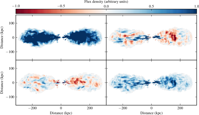
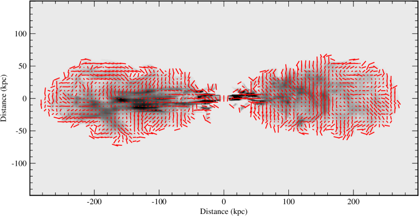
Figure 8: Full-resolution synchrotron images of B75-30-HR at $t=200$ Myr. Top row: Stokes $I$ (left) and $Q$ (right). Middle row: Stokes $U$ (left) and $P=\sqrt{Q^{2}+U^{2}}$ (right), colours as for top row. The mean Stokes $I$ is normalized to unity, so as to show faint structure, and this normalization is also applied to the other images. Bottom row: the same map (greyscale), with vectors whose length indicates fractional polarization and whose direction indicates the ‘magnetic field direction’.

One of the main aims of this paper was to extend the results of HE11, who found relatively high degrees of polarization in MHD simulations of radio galaxies in realistic environments. Our simulations allow high-resolution synchrotron imaging of Stokes $I$, $Q$ and $U$. To visualize synchrotron emission, we take all volume elements in the simulation with a value of the tracer quantity $>10^{-3}$, and then compute the emissivity in Stokes $I$, $Q$ and $U$ according to the relations given above (eqs 4–5, finally projecting along a chosen line of sight to form a two-dimensional image. Given the discussion of the previous section, such imaging is most likely to be realistic at late times when complex magnetic field structures have had a chance to develop.

Fig. 8 shows an example image, made from B75-30-HR; note in particular the filamentary structure in Stokes $I$ and the polarized intensity $P$ (see below, Section 3.7 for more on this) and the patchy, irregular appearance of Stokes $Q$ and $U$, a result of the complex magnetic field structure in the lobes at late times. Although the image shows the highest-resolution simulation, there is no very obvious difference between this and the other, lower-resolution runs in terms of the general properties of the images. The contour maps derived from these images (Fig. 8) are characteristic of the results of our simulations; the ‘magnetic field direction’ ($\theta_{m}=\frac{1}{2}\arctan(U/Q)+\pi/2$) is often parallel to the jet direction at the ends of the source, where backflow is most important, but perpendicular to the jet axis close to the core, where the toroidal field structure presumably dominates. It is this change in the characteristic field direction that presumably gives the low integrated fractional polarization (see Section 3.4). Similar behaviour is often seen in the lobes of real radio galaxies (Hardcastle et al., 1997). Fractional polarization is generally higher at the edges of the lobes than at the middle, again as seen by HE11 and also in real radio galaxies. (In this section we plot only results for sources lying at 90^∘ to the line of sight; results for smaller angles are qualitatively consistent with the results for sources in the plane of the sky, as also noted by HE11, and so are not shown here.)

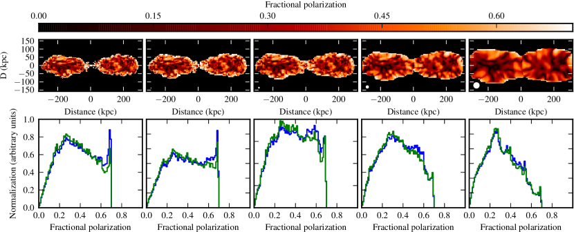
Figure 9: The effects of convolution on fractional polarization. Top panels show images of fractional polarization from B75-30-HR at $t=200$ Myr, while bottom panels show histograms of the distribution of fractional polarization with (green) and without (blue) the exclusion of the central injection region. From left to right: full resolution; convolved with a Gaussian of $\sigma=1$, 2, 4, 8 pixels.

It is important to consider how the source would appear if observed with a finite resolution (as is the case for real sources). This is illustrated in Fig. 9, where we plot the distribution of fractional polarization for B75-30-HR (which is representative of the general source population) at full resolution and smoothed with increasingly large Gaussians. The general effect of increasing the convolving beam size is to reduce the mean and maximum fractional polarization (unsurprisingly, since we have seen above that the unresolved sources are only marginally polarized). However, even beams that are an appreciable fraction of the source size give mean fractional polarizations around 30 per cent for these simulations. Our unsmoothed fractional polarization histograms are very comparable to those obtained by HE11 for their comparable simulations (light, fast jets at late times), confirming that their results are not simply the results of the lower numerical resolution of their simulations. The only important difference is the spike of points with the maximum possible fractional polarization in our data, which does not occur in the HE11 simulations. Imaging suggests that this is at least in part associated with the inner jet (as illustrated by the green histograms in Fig. 9, which show the polarization distribution when the injection region is excluded), and so part of the difference between our simulations and those of HE11 may arise from the different initial conditions for jet polarization in our simulations. Alternatively, since these very highly polarized regions are removed by convolution with a moderate-sized Gaussian beam, they must be small and so may be related to the higher numerical resolution of our simulations relative to those of HE11. These fractional polarization histograms are insensitive to the choice of tracer threshold, as long as it is not too close to unity – at thresholds $>0.1$ much of the lobe material disappears and the polarization seen is mostly that of the jet.

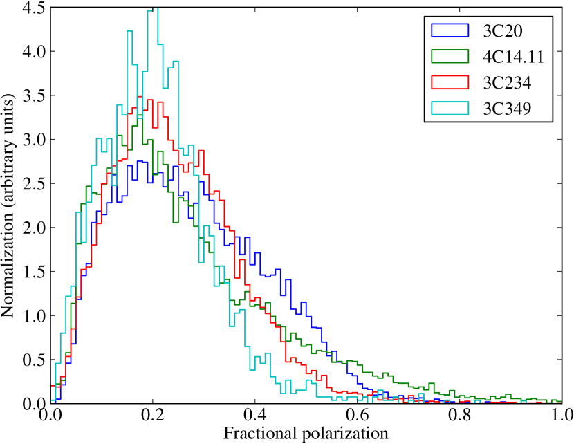
Figure 10: Fractional polarization histograms for four radio galaxies taken from Hardcastle et al. (1997).

How realistic are these distributions of fractional polarization? Fig. 10 shows fractional polarization histograms made at 8.4 GHz (a high enough frequency that rotation measure and depolarization should not be important) for four large, well-resolved radio galaxies from Hardcastle et al. (1997). It is important to note that these real histograms are affected by noise – which presumably accounts for the tail of fractional polarizations $\ga 0.7$ – as well as resolution effects. The resolution in the images used here is between 30 and 50 times the maximum source size, which means that the histograms should be compared with the final two panels of Fig. 9. On this basis, the agreement is quite good; both real and simulated histograms show peaks at fractional polarization around 20 to 30 per cent with a tail to larger values. A prediction from our work and that of HE11 is that high-resolution polarization maps of bright sources will tend to show higher fractional polarization, perhaps peaking around 40 per cent, and qualitatively this is indeed seen in higher-resolution maps; however, for a fair comparison, such maps will need to detect emission from the whole lobe, which is normally resolved out at the full resolution in low-sensitiviy maps such as those of Hardcastle et al. (1997). High-resolution ($LAS/\theta\sim 500$) fractional polarization imaging of Cygnus A (Perley & Carilli, 1996) does indeed show regions of very high fractional polarization in both lobes, but this source’s polarization properties are thought to be significantly affected by the rich intracluster medium, so a direct comparison with our simulations is difficult, though qualitatively the example of Cygnus A is encouraging; deep, high-resolution JVLA polarimetry of more typical radio galaxies is needed to give a better comparison with observations.

3.6 Rotation measure and depolarization

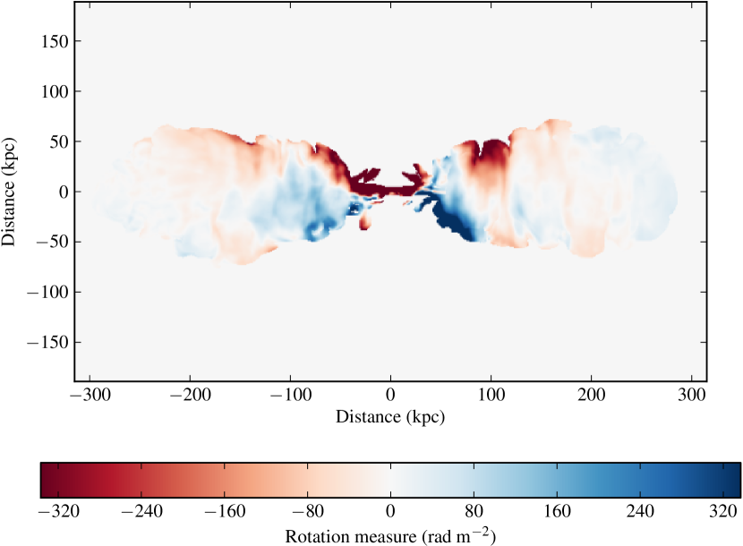
Figure 11: Example rotation measure visualization: B75-30-HR in the plane of the sky at $t=200$ Myr.

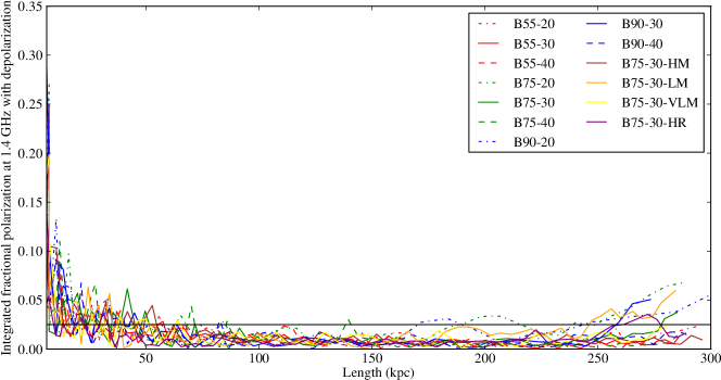
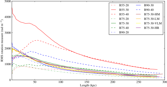
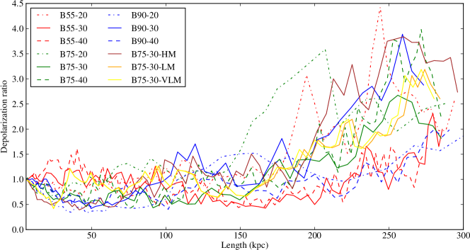
Figure 12: Effects of Faraday rotation as a function of lobe length. Top panel: integrated fractional polarization at 1.4 GHz. The solid black line shows the observed integrated 1.4-GHz fractional polarization of unresolved steep-spectrum sources (Tucci et al., 2004). Middle panel: RMS value of the rotation measure in RM images. Bottom panel: depolarization ratio for lobes at 45^∘ to the line of sight (the Laing-Garrington effect). B75-30-HR is omitted from the bottom panel as a uniform path length through the shocked external medium cannot be achieved at late times.

A magnetised intracluster medium gives rise to Faraday rotation which (if wholly or partially unresolved) will lead to depolarization (Burn, 1966; Laing, 1984). Here we are only concerned with external depolarization, the effect of the medium between the radio lobe and the observer, as there is little direct evidence for internal depolarization in FRII lobes, and we cannot in any case adequately model the microphysics of thermal entrainment in FRIIs.

The rotation measure ($RM$) is defined as

$$RM=C\int n_{\rm th}B_{\parallel}{\rm d}z\ {\rm rad}\ {\rm m}^{-2}$$ (6)

where $C$ is a constant which in physical units is $2.62\times 10^{-13}$ T^-1, $n_{\rm th}$ is the thermal density and $B_{\parallel}$ is the component of magnetic field parallel to the line of sight. The actual angle of Faraday rotation in radians is then given by $\phi=RM\lambda^{2}$, where $\lambda$ is the wavelength of observation. As we have chosen the values of our field strength and density to match observed properties of clusters of this type, we can easily compute $RM$, and so $\phi$, in physical units.

We visualize rotation measure by integrating as specified by eq. 6 from an outer radius defined by the edge of the computational volume along the $x$ axis (320 kpc) along the line of sight until the near edge of the lobes is reached (defined as usual using tracer values $>10^{-3}$). This allows maps of RM to be constructed (Fig. 11). Huarte-Espinosa et al. (2011b) have discussed such synthetic RM images in detail and it is not our purpose in this paper to repeat their analysis. However, we are exploring a rather different regime of cluster parameter space – our sources are physically larger at the grid edges, considerably lower in jet power, and inhabit clusters/groups with smaller core radii. As a result, we would in general expect lower values of the rotation measure at late times, which is indeed what we observe. A characteristic size scale of the structures in RM of order tens of kpc is observed, which, given that the largest scale of the power spectrum of the magnetic field is 40–80 kpc, is consistent with the estimates of the coherence length for RM in the undisturbed ICM given by Cho & Ryu (2009). We also note in some, though not all, simulated sources a tendency for a systematic side-to-side asymmetry in RM, which we attribute to the predominantly toroidal field of the radio galaxy ‘leaking’ (either via small-scale mixing at the boundary layer or numerically) into the shocked material; this is not so obvious in the maps of Huarte-Espinosa et al. (2011b), though there are hints that it may be present in the lightest-jet simulations which are the best match to those we use here. This effect is independent of tracer threshold and so is not simply an effect of lobe material which is not being classified as such; it appears to be important where the edge of the lobe becomes K-H unstable, giving rise to fine structure and numerical mixing at the lobe boundary. However, as the effect can be removed by cutting off the RM integration within a few volume elements of the lobe boundary without significantly affecting the range or dispersion of the RM, we ignore it in the analysis that follows.

Rotation measure causes depolarization if it is unresolved or partially resolved. It has a particularly strong effect on integrated polarization, as defined in Section 3.4. Fig. 12 (top panel) shows the results of ‘observing’ at 1.4 GHz (chosen as it is the frequency of the FIRST and NVSS surveys) taking the effects of rotation measure into account. The fractional polarization is reduced to low levels, almost independent of source size, by the depolarization from the intracluster medium; we do not expect in practice to see the high levels of integrated polarization shown in Fig. 7. The integrated fractional polarization plotted is now consistent with the observational value. Fig. 12 also shows the RMS value of rotation measure seen by the lobes (at 90 degrees to the line of sight) and, as expected, we see that this generally decreases with time and is larger for sources in denser environments. The non-negligible values of $<RM^{2}>^{1/2}$ even for large sources means that we can expect substantial rotation/depolarization in low-frequency polarization observations of such objects.

Finally, we can estimate the magnitude of the Laing-Garrington effect (Laing, 1988; Garrington et al., 1988, 1991) for our sources. The Laing-Garrington effect is the tendency of the jetted (therefore nearer) lobe to be less depolarized than the counterjet (further) lobe, as a result of the longer path length to the further lobe through the depolarizing medium. Although X-ray observations are consistent with the observed polarization properties of radio sources in a few cases (Belsole et al., 2007) there has been no systematic observational comparison between polarization statistics and group/cluster properties; our simulations allow us to make some predictions. We simulate the observations described by Garrington et al. (1991) by considering lobes at 45^∘ to the line of sight, generating and applying the RM map at two frequencies of 1.4 and 5 GHz, and then convolving with a Gaussian designed to give roughly 15 beam widths across the source (matching the observations of Garrington et al. 1991). The resolved fractional polarization is then measured for each lobe at each frequency, the depolarization ($DP=f_{\rm 1.4}/f_{5}$ is calculated for the two lobes, and finally we compute the depolarization ratio, $DPR=DP_{j}/DP_{cj}$, where the ‘jet’ and ‘counterjet’ lobes are simply taken to be those closer to and further away from the observer. $DPR$ by this definition should be larger than 1 to be in the sense expected from the Laing-Garrington effect. The results are plotted in Fig. 12 and it can be seen that a Laing-Garrington effect at these frequencies is indeed expected even for these relatively poor environments, especially for large lobe lengths. The magnitude of $DPR$ is very comparable to what is found in observations. Two other points are worth noting about this plot; the comparatively large scatter and the lack of a strong Laing-Garrington signal at small lobe lengths. The scatter is perhaps not surprising, as with each time step the lobe is advancing into a new part of the external medium with potentially different magnetic field structure (recall the turbulent initial magnetic field conditions) but shows that the absolute magnitude of the Laing-Garrington effect in individual sources will be hard to use to infer physical conditions for the intracluster medium; resolved depolarization/RM imaging will in general be far more robust for these purposes. The lack of a strong effect at small lobe lengths is perhaps surprising given that Garrington et al. (1991) report stronger Laing-Garrington signals for sources of small angular size, but of course small angular sizes also tend to be associated with more distant, more luminous objects plausibly in richer X-ray environments (cf. Ineson et al. (2013)) which might then have higher DPR for a given physical size. Additionally, there may be some difficulty in imaging the Laing-Garrington effect in our simulations at small angles to the line of sight due to the large source axial ratios at early times.

3.7 Inverse-Compton visualization

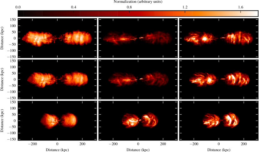
Figure 13: Inverse-Compton and synchrotron visualizations of B75-30-HR at $t=200$ Myr. From top to bottom, the simulation is at 0^∘, 30^∘ and 60^∘ to the plane of the sky. Left panel: inverse-Compton; centre panel: synchrotron; right panel: synchrotron divided by inverse-Compton. The colour scale is linear with arbitrary units.

We can very easily visualize inverse-Compton scattering of the CMB in these models by simply integrating particle (thermal) pressure along the line of sight (as before we require values of the tracer $>10^{-3}$ for this analysis). The CMB is an isotropic photon field and is scattered by low-energy electrons whose number density will be strictly correlated with the local value of pressure (unless there is an energetically dominant, spatially varying proton population: see discussion in Section 4.1). By doing this we can compare with the few existing results on the resolved relationship between inverse-Compton and synchrotron emission (Hardcastle & Croston, 2005; Goodger et al., 2008).

Results of this analysis for B75-30-HR are shown in Fig. 13. Again, while we use the high-resolution simulation for display purposes, these images are representative of all of our simulations. Here we plot three angles to the line of sight to show that our conclusions are not strongly affected by viewing angle. We see that the simulated inverse-Compton emission is much more uniform across the lobe than the synchrotron emission, exactly as seen in real sources such as Pictor A (Hardcastle & Croston, 2005): consequently, the ratio of synchrotron to inverse-Compton, which essentially represents the pressure-weighted projection of the magnetic field terms in eq. 4, exhibits strong structure. Clearly this arises because the magnetic field (or more precisely the energy density in the components perpendicular to the line of sight, see eq. 4) is very much more intermittent than the pressure. Tregillis et al. (2004), who also simulated light, fast jets, obtained similar results, in the sense that the scatter in their synchrotron flux was very much larger than the scatter in their inverse-Compton flux, and Gaibler (2008) finds a similarly smooth appearance in inverse-Compton visualizations of axisymmetric lobes, so we suggest that this is a general feature of MHD models where the field is not dynamically important. We would argue therefore that these simulations strongly support the arguments of e.g. Hardcastle & Croston (2005) and Hardcastle (2013): filamentary structures seen in total intensity synchrotron radiation are primarily tracing intermittency of the magnetic field and can be used to derive information on the magnetic field power spectrum.

It can readily be seen that the total inverse-Compton emissivity in these models (and for this visualization) scales with $\int P{\rm d}V$ and so essentially traces the total thermal energy in the lobes, which increases linearly with time (Section 3.3). Thus we expect large, old sources in poor environments where the synchrotron emission has passed its peak (Section 3.4) to have larger ratios of inverse-Compton to low-frequency synchrotron emission, irrespective of the ratio of magnetic to particle energy of the lobe (which is in fact roughly constant in these simulations at all but the earliest times: Fig. 2).

4 Discussions and conclusions

4.1 Critique

We should begin by acknowledging the ways in which our simulations are not representative of real radio galaxies, since this helps us to understand the extent to which our results tell us about real observations.

Although we have tuned the simulation parameters to match those of real sources as closely as possible within our numerical limitations, we are almost certainly some way off reality in the lobes. In FRIIs there is no evidence for an energetically dominant (thermal or non-thermal) proton population (Croston et al., 2005). The absence of thermal content in the lobes means that the effective matter density in lobes is very low indeed, $\sim 3p/c^{2}$. For $p\sim 10^{-11}$ Pa (the pressure in the centre of our environments) the matter density would be equivalent to 0.2 protons m^-3, or about a factor $10^{5}$ below the ambient central density; our lobes have a density contrast at most a little above $10^{4}$ (Fig. 1). The equation of state is also wrong in the lobes – even the observed density contrast implies temperatures $10^{4}$ times higher than ambient for rough pressure balance, and thus $kT=20$ MeV, implying relativistic electrons and a ratio of specific heats of $\frac{4}{3}$. And, possibly most importantly, the speed of the jet is high enough ($0.24c$) that relativistic effects would ideally be taken account of in the modelling, but at the same time too low to match observations, which require a minimum of $\sim 0.5c$ (Mullin & Hardcastle, 2009) and maybe $>0.99c$ (Konar & Hardcastle, 2013, and references therein). We could only accommodate such high speeds while maintaining the jet energetics and high density contrast by reducing the input jet radius, which would improve the realism of the simulations (a jet radius of a few kpc is certainly too large on the smallest scales we probe) but this would require higher numerical resolution for adequate modelling, as well as the use of relativistic codes.

A consequence of our choice to limit the speed is that the jet is only mildly supersonic with respect to its internal sound speed. Consequently, there is no strong jet termination shock, and our simulations do not form bright hotspots, though there are weak transient shock structures within the lobes at various times. In fact, synchrotron visualizations of the lobes (Fig. 8) tend to show structures related to the jet, i.e. to have an FRI-like or intermediate FRI/II structure, not unlike some real radio sources (e.g. Hercules A, Gizani & Leahy 2003) but certainly not typical of the FRII population. Since the lobe dynamics are dependent on ram pressure balance at the front of the lobe and on the lobe temperature and density, none of which depend explicitly on the jet internal Mach number, we would argue that this does not affect our ability to understand lobe dynamics and energetics, but it may affect our conclusions about observability.

Turning to physics that is absent altogether, the most important missing piece of the picture is particle acceleration and loss, which is well known to be important in real radio galaxies – we have the capability to map this in great detail in observations with the current generation of radio telescopes (Harwood et al., 2013). Including acceleration processes would certainly increase the visibility of hotspots (see the simulations of e.g. Tregillis et al. (2001) where these processes are taken into account, or those of Krause et al. (2012) where a shock tracer is used to infer high-frequency emissivity) while including radiative losses would also affect our modelling of the evolution of lobe radio luminosity (Section 3.4) although, again, neither of them would affect the dynamics significantly (the total energy radiated away by a radio galaxy in its lifetime is only a small fraction of what is stored in the lobes). Of course, in order to model acceleration processes usefully, we would need more strongly supersonic speeds in the jet, as discussed above, together with some prescription for particle acceleration at internal shocks. Cooling in the intracluster medium is also not taken into account, though this is less important for the simulated media we have used and the lifetimes of the sources ($\sim 10^{8}$ years).

4.2 What we have learnt

We can now summarize what we think these new simulations tell us, bearing in mind the limitations imposed by the discussion of the previous section.

• The broad dynamical conclusions of Paper I, as expected, are reproduced (Section 3.2): lobes of this type are not self-similar and come into rough pressure equilibrium with their surroundings. Lobes are driven away from the centre of the cluster environment at late times by the return of the dense central cluster material. As the lobes are effectively vacuum, the fact that we have not achieved realistic values of the density contrast probably will not significantly affect this conclusion.

• One of the key conclusions of Paper I, that the models imply rough energy equipartition between the lobes and the shocked material surrounding them, is robust (Section 3.3) – it is hard to see how this could depend on the details of the jet dynamics or the density contrast, although the lobe equation of state would be expected to affect it to some extent and, as noted above, we are not yet simulating jets of the correct speed or internal Mach number. It almost certainly does depend on the lobes coming into pressure balance, and would not be expected to be true in the early, strong-shock regime (cf. Cielo et al. (2014)).

• Another conclusion of Paper I, that the evolution of radio luminosity should be strongly affected by environment, is reproduced here (Section 3.4). Our tracks in the power/linear size diagram (Fig. 7) are probably more realistic than those of Paper I because of our more realistic source dynamics at early times and because of the inclusion of magnetic fields: they still show close to an order of magnitude difference, for a given length, between sources of identical intrinsic jet power, which, as discussed in Paper I, renders radio-luminosity-based estimates of jet kinetic power $Q$ very uncertain. Because the integrated luminosity depends largely on the lobe volume and pressure, this conclusion cannot be sensitive to details of the jet dynamics in the regime where the lobe is in rough pressure balance. Of course, loss and acceleration processes would significantly change the shape of these curves at high frequency, but they would be very unlikely to do so in such a way as to bring them into systematically closer agreement.

• Lobes with a magnetic field that is not dynamically dominant, given any reasonable initial field configuration, rather naturally evolve towards a state where the energies in the toroidal and longitudinal field components are of the same order of magnitude, arising because of the balance between the growth of the toroidal field through the ‘toroidal stretching process’ (Matthews & Scheuer 1990; Gaibler et al. 2009; HE11) and the effects of shearing of the toroidal field from jet and backflow (Section 3.1, 3.3) which together give rise to a predominantly longitudinal component with many field reversals. (The growth of this disordered longitudinal component is presumably limited by reconnection on the smallest scales, though our results do not appear to be strongly-resolution-dependent.) The presence of these two significant field components gives rise to complex polarization structure at all late times in the simulations (i.e. at all times when large-scale bulk motions within the lobes are capable of operating), as also seen by HE11, so long as the initial field is not too weak. These processes can only be studied in 3D. Here the limitations of our simulations are related to the internal bulk speeds and densities and our assumptions about the initial field configuration and strength, but, so long as the field does not become dynamically dominant, it is hard to see how these could make a qualitative difference.

• The complex field configuration that we observe (and that has been observed previously by e.g. Tregillis et al. (2004) and HE11 gives rise to a number of important features of the total and polarized emission. First of all, we note that filamentary structure seen in total intensity (e.g. Fig. 8) is almost entirely due to intermittency in the magnetic field. In fact, we can take out the variation in the line-of-sight electron pressure altogether (Fig. 13) and still see all the filamentation, as HE11 also remark. This is in fact very natural in a situation where the magnetic field is not dynamically dominant – pressure variations in the electrons will be washed out on a sound-crossing time (for the high internal sound speed of the lobes) while magnetic filaments can persist and grow. An observational consequence of this is that inverse-Compton visualizations show a much smoother structure than synchrotron (Section 3.7). There is some direct evidence from observation that this is the case in real radio galaxies (Hardcastle & Croston, 2005).

• Turning to polarized emission, we see that the complex polarization structure at late times implies low integrated polarization (Section 3.4) as observed. (Conversely, the high integrated fractional polarization implied by our simulations at early times, before the lobe internal dynamics have had any effect on the field, is probably not realistic, although, as discussed in Section 3.6, it would probably be washed out by Faraday effects in any case.) However, the fact that large-scale magnetic field structures have a strong effect on emissivity means that there are expected to be regions of the lobe with high fractional polarization (Section 3.5). We have compared observed and simulated fractional polarization for the first time, finding good qualitative agreement, but we predict that as high-resolution, sensitive polarization observations of lobes become available, the maximum polarization seen will approach the theoretical maximum, with a complex relationship between structures in total intensity and polarization (Fig. 8). These results confirm the work of HE11 with numerical resolution up to a factor 3 higher.

• Finally, we have briefly investigated resolved depolarization effects of the magnetized external medium on the lobes, following Huarte-Espinosa et al. (2011b). We reproduce the Laing-Garrington effect in a numerical model, the first time that this has been done, and so demonstrate that the physical conditions in even a moderate-density environment are capable of producing a significant Laing-Garrington effect at GHz frequencies (Section 3.6). The ability to model depolarization effects of this type will become increasingly important with the advent of low-frequency polarimetry. We caution that some of the quantitative detail discussed here (e.g. the way in which the Laing-Garrington effect only becomes important with source sizes comparable to the core radius) depends on the lobe dynamics at small scales and our assumptions about the cluster magnetic field strength and power spectrum, which may not be realistic.

In future work, we plan to verify these conclusions for more realistic (i.e. not spherically symmetric) cluster environments and include the effects of particle acceleration and loss in our modelling, with the ultimate aim of generating recipes by which jet power and source environment can be inferred accurately from multi-frequency, resolved, full-polarization images of radio galaxies.

REFERENCES

- Basson & Alexander (2003) Basson J. F., Alexander P., 2003, MNRAS, 339, 353
- Belsole et al. (2007) Belsole E., Worrall D. M., Hardcastle M. J., Croston J. H., 2007, MNRAS, 381, 1109
- Black et al. (1992) Black A. R. S., Baum S. A., Leahy J. P., Perley R. A., Riley J. M., Scheuer P. A. G., 1992, MNRAS, 256, 186
- Bridle et al. (1994) Bridle A. H., Hough D. H., Lonsdale C. J., Burns J. O., Laing R. A., 1994, AJ, 108, 766
- Burn (1966) Burn B. J., 1966, MNRAS, 133, 67
- Cho & Ryu (2009) Cho J., Ryu D., 2009, ApJ, 705, L90
- Chon et al. (2012) Chon G., Böhringer H., Krause M., Trümper J., 2012, A&A, 545, L3
- Cielo et al. (2014) Cielo S., Antonuccio-Delogu V., Macciò A. V., Romeo A. D., Silk J., 2014, MNRAS
- Clarke et al. (1989) Clarke D. A., Burns J. O., Norman M. L., 1989, ApJ, 342, 700
- Croston et al. (2005) Croston J. H., Hardcastle M. J., Harris D. E., Belsole E., Birkinshaw M., Worrall D. M., 2005, ApJ, 626, 733
- Fanaroff & Riley (1974) Fanaroff B. L., Riley J. M., 1974, MNRAS, 167, 31P
- Gaibler (2008) Gaibler V., 2008, PhD thesis, ZAH / Landessternwarte, University of Heidelberg, Germany
- Gaibler et al. (2011) Gaibler V., Khochfar S., Krause M., 2011, MNRAS, 411, 155
- Gaibler et al. (2012) Gaibler V., Khochfar S., Krause M., Silk J., 2012, MNRAS, 425, 438
- Gaibler et al. (2009) Gaibler V., Krause M., Camenzind M., 2009, MNRAS, 400, 1785
- Garrington et al. (1988) Garrington S., Leahy J. P., Conway R. G., Laing R. A., 1988, Nature, 331, 147
- Garrington et al. (1991) Garrington S. T., Conway R. G., Leahy J. P., 1991, MNRAS, 250, 171
- Gizani & Leahy (2003) Gizani N. A. B., Leahy J. P., 2003, MNRAS, 342, 399
- Goodger et al. (2008) Goodger J. L., Hardcastle M. J., Croston J. H., Kassim N., Perley R. A., 2008, MNRAS, 386, 337
- Guidetti et al. (2012) Guidetti D., Laing R. A., Croston J. H., Bridle A. H., Parma P., 2012, MNRAS, 423, 1335
- Hardcastle (2013) Hardcastle M. J., 2013, MNRAS, 433, 3364
- Hardcastle et al. (1997) Hardcastle M. J., Alexander P., Pooley G. G., Riley J. M., 1997, MNRAS, 288, 859
- Hardcastle et al. (2001) Hardcastle M. J., Birkinshaw M., Worrall D. M., 2001, MNRAS, 323, L17
- Hardcastle & Croston (2005) Hardcastle M. J., Croston J. H., 2005, MNRAS, 363, 649
- Hardcastle & Krause (2013) Hardcastle M. J., Krause M. G. H., 2013, MNRAS, 430, 174
- Hardcastle & Worrall (2000) Hardcastle M. J., Worrall D. M., 2000, MNRAS, 319, 562
- Harwood et al. (2013) Harwood J. J., Hardcastle M. J., Croston J. H., Goodger J. L., 2013, MNRAS, 435, 3353
- Heinz et al. (2006) Heinz S., Brüggen M., Young A., Levesque E., 2006, MNRAS, 373, L65
- Huarte-Espinosa et al. (2011a) Huarte-Espinosa M., Krause M., Alexander P., 2011a, MNRAS, 417, 382
- Huarte-Espinosa et al. (2011b) Huarte-Espinosa M., Krause M., Alexander P., 2011b, MNRAS, 418, 1621
- Ineson et al. (2013) Ineson J., Croston J. H., Hardcastle M. J., Kraft R. P., Evans D. A., Jarvis M., 2013, ApJ, 770, 136
- Kaiser & Alexander (1997) Kaiser C. R., Alexander P., 1997, MNRAS, 286, 215
- Kataoka & Stawarz (2005) Kataoka J., Stawarz Ł., 2005, ApJ, 622, 797
- Konar & Hardcastle (2013) Konar C., Hardcastle M. J., 2013, MNRAS, 436, 1595
- Kraft et al. (2007) Kraft R. P., Birkinshaw M., Hardcastle M. J., Evans D. A., Croston J. H., Worrall D. M., Murray S. S., 2007, ApJ, 659, 1008
- Kraft et al. (2006) Kraft R. P., Jones C., Nulsen P. E. J., Hardcastle M. J., 2006, ApJ, 640, 762
- Krause (2003) Krause M., 2003, A&A, 398, 113
- Krause (2005) Krause M., 2005, A&A, 431, 45
- Krause et al. (2012) Krause M., Alexander P., Riley J., Hopton D., 2012, MNRAS, 427, 3196
- Laing (1984) Laing R. A., 1984, in Physics of Energy Transport in Radio Galaxies, Bridle A.H., Eilek J.A., ed., NRAO Workshop no. 9, NRAO, Green Bank, West Virginia, p. 90
- Laing (1988) Laing R. A., 1988, Nature, 331, 149
- Leahy et al. (1997) Leahy J. P., Black A. R. S., Dennett-Thorpe J., Hardcastle M. J., Komissarov S., Perley R. A., Riley J. M., Scheuer P. A. G., 1997, MNRAS, 291, 20
- Matthews & Scheuer (1990) Matthews A. P., Scheuer P. A. G., 1990, MNRAS, 242, 623
- Mendygral et al. (2012) Mendygral P. J., Jones T. W., Dolag K., 2012, ApJ, 750, 166
- Mignone et al. (2007) Mignone A., Bodo G., Massaglia S., Matsakos T., Tesileanu O., Zanni C., Ferrari A., 2007, ApJS, 170, 228
- Mignone et al. (2010) Mignone A., Rossi P., Bodo G., Ferrari A., Massaglia S., 2010, MNRAS, 402, 7
- Mullin & Hardcastle (2009) Mullin L. M., Hardcastle M. J., 2009, MNRAS, 398, 1989
- Murgia et al. (2004) Murgia M., Govoni F., Feretti L., Giovannini G., Dallacasa D., Fanti R., Taylor G. B., Dolag K., 2004, A&A, 424, 429
- O’Neill & Jones (2010) O’Neill S. M., Jones T. W., 2010, ApJ, 710, 180
- O’Neill et al. (2005) O’Neill S. M., Tregillis I. L., Jones T. W., Ryu D., 2005, ApJ, 633, 717
- Perley & Carilli (1996) Perley R. A., Carilli C. L., 1996, in Cygnus A — Study of a Radio Galaxy, Carilli C.L., Harris D.E., ed., Cambridge University Press, Cambridge, p. 168
- Reynolds et al. (2002) Reynolds C. S., Heinz S., Begelman M. C., 2002, MNRAS, 332, 271
- Tregillis et al. (2001) Tregillis I. L., Jones T. W., Ryu D., 2001, ApJ, 557, 475
- Tregillis et al. (2004) Tregillis I. L., Jones T. W., Ryu D., 2004, ApJ, 601, 778
- Tucci et al. (2004) Tucci M., Martínez-González E., Toffolatti L., González-Nuevo J., De Zotti G., 2004, MNRAS, 349, 1267
- Wagner & Bicknell (2011) Wagner A. Y., Bicknell G. V., 2011, ApJ, 728, 29
- Wagner et al. (2012) Wagner A. Y., Bicknell G. V., Umemura M., 2012, ApJ, 757, 136
- Wilson et al. (2006) Wilson A. S., Smith D. A., Young A. J., 2006, ApJ, 644, L9
- Zanni et al. (2003) Zanni C., Bodo G., Rossi P., Massaglia S., Durbala A., Ferrari A., 2003, A&A, 402, 949