STAIR Codes: A General Family of Erasure Codes for Tolerating Device and Sector Failures

Abstract

Practical storage systems often adopt erasure codes to tolerate device failures and sector failures, both of which are prevalent in the field. However, traditional erasure codes employ device-level redundancy to protect against sector failures, and hence incur significant space overhead. Recent sector-disk (SD) codes are available only for limited configurations. By making a relaxed but practical assumption, we construct a general family of erasure codes called STAIR codes, which efficiently and provably tolerate both device and sector failures without any restriction on the size of a storage array and the numbers of tolerable device failures and sector failures. We propose the upstairs encoding and downstairs encoding methods, which provide complementary performance advantages for different configurations. We conduct extensive experiments on STAIR codes in terms of space saving, encoding/decoding speed, and update cost. We demonstrate that STAIR codes not only improve space efficiency over traditional erasure codes, but also provide better computational efficiency than SD codes based on our special code construction. Finally, we present analytical models that characterize the reliability of STAIR codes, and show that the support of a wider range of configurations by STAIR codes is critical for tolerating sector failure bursts discovered in the field.

1 Introduction

Mainstream disk drives are known to be susceptible to both device failures [30, 42] and sector failures [1, 41]: a device failure implies the loss of all data in the failed device, while a sector failure implies the data loss in a particular disk sector. In particular, sector failures are of practical concern not only in disk drives, but also in emerging solid-state drives (SSDs) as they often appear as worn-out blocks after frequent program/erase cycles [17, 9, 18, 48]. In the face of device and sector failures, practical storage systems often adopt erasure codes to provide data redundancy [37]. However, existing erasure codes often build on tolerating device failures and provide device-level redundancy only. To tolerate additional sector failures, an erasure code must be constructed with extra parity disks. A representative example is RAID-6, which uses two parity disks to tolerate one device failure together with one sector failure in another non-failed device [44, 25]. If the sector failures can span a number of devices, the same number of parity disks must be provisioned. Clearly, dedicating an entire parity disk for tolerating a sector failure is too extravagant.

To tolerate both device and sector failures in a space-efficient manner, sector-disk (SD) codes [33, 32] and the earlier PMDS codes [5] (which are a subset of SD codes) have recently been proposed. Their idea is to introduce parity sectors, instead of entire parity disks, to tolerate a given number of sector failures. However, the constructions of SD codes are known only for limited configurations (e.g., the number of tolerable sector failures is no more than three), and some of the known constructions rely on exhaustive searches [33, 32, 7]. An open issue is to provide a general construction of erasure codes that can efficiently tolerate both device and sector failures without any restriction on the size of a storage array, the number of tolerable device failures, or the number of tolerable sector failures.

In this paper, we make the first attempt to develop such a generalization, which we believe is of great theoretical and practical interest to provide space-efficient fault tolerance for today’s storage systems. After carefully examining the assumption of SD codes on failure coverage, we find that although SD codes have relaxed the assumption of the earlier PMDS codes to comply with how most storage systems really fail, the assumption remains too strict. By reasonably relaxing the assumption of SD codes on sector failure coverage, we construct a general family of erasure codes called STAIR codes, which efficiently tolerate both device and sector failures.

Specifically, SD codes devote $s$ sectors per stripe to coding, and tolerate the failure of any $s$ sectors per stripe. We relax this assumption in STAIR codes by limiting the number of devices that may simultaneously contain sector failures, and by limiting the number of simultaneous sector failures per device. Consequently, as shown in §2, STAIR codes are constructed to protect the sector failure coverage defined by a vector $\mathbf{e}$, rather than all combinations of $s$ sector failures.

With the relaxed assumption, the construction of STAIR codes can be based on existing erasure codes. For example, STAIR codes can build on Reed-Solomon codes (including standard Reed-Solomon codes [39, 31, 35] and Cauchy Reed-Solomon codes [8, 38]), which have no restriction on code length and fault tolerance.

We first define some basic concepts and elaborate how the sector failure coverage is formulated for STAIR codes in §2. Then the paper makes the following contributions:

• We present a baseline construction of STAIR codes. Its idea is to run two orthogonal encoding phases based on Reed-Solomon codes. See §3.

• We propose an upstairs decoding method, which systematically reconstructs the lost data due to both device and sector failures. The proof of fault tolerance of STAIR codes follows immediately from the decoding method. See §4.

• Inspired by upstairs decoding, we extend the construction of STAIR codes to regularize the code structure. We propose two encoding methods: upstairs encoding and downstairs encoding, both of which reuse computed parity results in subsequent encoding. The two encoding methods provide complementary performance advantages for different configuration parameters. See §5.

• We extensively evaluate STAIR codes in terms of space saving, encoding/decoding speed, and update cost. We show that STAIR codes achieve significantly higher encoding/decoding speed than SD codes through parity reuse. Most importantly, we show the versatility of STAIR codes in supporting any size of a storage array, any number of tolerable device failures, and any number of tolerable sector failures. See §6.

• We develop analytical models to characterize the reliability of STAIR codes and discuss how the sector failure coverage of STAIR codes should be configured. We examine both independent and correlated sector failure models, and show that it is critical for STAIR codes to support a wider range of configurations in the presence of sector failure bursts discovered in the field [1, 41]. See §7.

We review related work in §8, and conclude this paper in §9.

2 Preliminaries

This section presents the definitions and the problem of simultaneous device and sector failures in storage arrays. Table 1 summarizes the major notation used for the STAIR code construction.

Table 1: Major notation used for the STAIR code construction.

Notation	Description
Defined in §2:
$n$	Number of chunks per stripe (i.e. number of devices per storage array)
$r$	Number of sectors (i.e. symbols) per chunk
$m$	Maximum number of entirely failed chunks (due to device failures) per stripe
$m^{\prime}$	Maximum number of partially failed chunks (due to sector failures) per stripe
$\mathbf{e}$	Sector failure coverage, defined as $\mathbf{e}=(e_{0},e_{1},\cdots,e_{m^{\prime}-1})$ (where $0<e_{0}\leq e_{1}\leq\cdots\leq e_{m^{\prime}-1}\leq r$)
$s$	Maximum number of sector failures per stripe, defined as $s=\sum_{i=0}^{m^{\prime}-1}e_{i}$
Defined in §3:
$d_{i,j}$	Data symbol (where $0\leq i\leq r-1$, and $0\leq j\leq n-m-1$)
$p_{i,k}$	Row parity symbol (where $0\leq i\leq r-1$, and $0\leq k\leq m-1$)
$p^{\prime}_{i,l}$	Intermediate parity symbol (where $0\leq i\leq r-1$, and $0\leq l\leq m^{\prime}-1$)
$g_{h,l}$	Outside global parity symbol (where $0\leq l\leq m^{\prime}-1$, and $0\leq h\leq e_{l}-1$)
$\mathcal{C}_{row}$	Systematic MDS code for encoding in row direction
$\mathcal{C}_{col}$	Systematic MDS code for encoding in column direction
Defined in §4:
$d^{*}_{h,j}$	Virtual parity symbol encoded from a data chunk (where $0\leq h\leq e_{l}-1$, and $0\leq j\leq n-m-1$)
$p^{*}_{h,k}$	Virtual parity symbol encoded from a row parity chunk (where $0\leq h\leq e_{l}-1$, and $0\leq k\leq m-1$)
Defined in §5:
$\hat{g}_{h,l}$	Inside global parity symbol (where $0\leq l\leq m^{\prime}-1$, and $0\leq h\leq e_{l}-1$)

We consider a storage array with $n$ devices, each of which has its storage space logically segmented into a sequence of continuous chunks (also called strips) of the same size. We group each of the $n$ chunks at the same position of each device into a stripe, as depicted in Figure 1. Each chunk is composed of $r$ sectors. Thus, we can view the stripe as a $r\times n$ array of sectors. Using coding theory terminology, we refer to each sector as a symbol. Each stripe is independently protected by an erasure code for fault tolerance, so our discussion focuses on a single stripe.

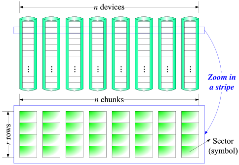
Figure 1: A stripe for $n=8$ and $r=4$.

Storage arrays are subject to both device and sector failures. A device failure can be mapped to the failure of an entire chunk of a stripe. We assume that the stripe can tolerate at most $m$ ($<n$) chunk failures, in which all symbols are lost. In addition to device failures, we assume that sector failures can occur in the remaining $n-m$ devices. Each sector failure is mapped to a lost symbol in the stripe. Suppose that besides the $m$ failed chunks, the stripe can tolerate sector failures in at most $m^{\prime}$ ($\leq n-m$) remaining chunks, each of which has a maximum number of sector failures defined by a vector $\mathbf{e}=(e_{0},e_{1},\cdots,e_{m^{\prime}-1})$. Without loss of generality, we arrange the elements of $\mathbf{e}$ in monotonically increasing order (i.e., $e_{0}\leq e_{1}\leq\cdots\leq e_{m^{\prime}-1}$). For example, suppose that sector failures can only simultaneously appear in at most three chunks (i.e., $m^{\prime}=3$), among which at most one chunk has two sector failures and the remaining have one sector failure each. Then, we can express $\mathbf{e}=(1,1,2)$. Also, let $s=\sum_{i=0}^{m^{\prime}-1}e_{i}$ be the total number of sector failures defined by $\mathbf{e}$. Our study assumes that the configuration parameters $n$, $r$, $m$, and $\mathbf{e}$ (which then determines $m^{\prime}$ and $s$) are the inputs selected by system practitioners for the erasure code construction.

Erasure codes have been used by practical storage systems to protect against data loss [37]. We focus on a class of erasure codes with optimal storage efficiency called maximum distance separable (MDS) codes, which are defined by two parameters $\eta$ and $\kappa$ ($<\eta$). We define an $(\eta,\kappa)$-code as an MDS code that transforms $\kappa$ symbols into $\eta$ symbols collectively called a codeword (this operation is called encoding), such that any $\kappa$ of the $\eta$ symbols can be used to recover the original $\kappa$ uncoded symbols (this operation is called decoding). Each codeword is encoded from $\kappa$ uncoded symbols by multiplying a row vector of the $\kappa$ uncoded symbols with a $\kappa\times\eta$ generator matrix of coefficients based on Galois Field arithmetic. We assume that the $(\eta,\kappa)$-code is systematic, meaning that the $\kappa$ uncoded symbols are kept in the codeword. We refer to the $\kappa$ uncoded symbols as data symbols, and the $\eta-\kappa$ coded symbols as parity symbols. We use systematic MDS codes as the building blocks of STAIR codes. Examples of such codes are standard Reed-Solomon codes [39, 31, 35] and Cauchy Reed-Solomon codes [8, 38].

Given parameters $n$, $r$, $m$, and $\mathbf{e}$ (and hence $m^{\prime}$ and $s$), our goal is to construct a STAIR code that tolerates both $m$ failed chunks and $s$ sector failures in the remaining $n-m$ chunks defined by $\mathbf{e}$. Note that some special cases of $\mathbf{e}$ have the following physical meanings:

• If $\mathbf{e}=(1)$, the corresponding STAIR code is equivalent to a PMDS/SD code with $s=1$ [5, 33, 32]. In fact, the STAIR code is a new construction of such a PMDS/SD code.

• If $\mathbf{e}=(r)$, the corresponding STAIR code has the same function as a systematic $(n,n-m-1)$-code.

• If $\mathbf{e}=(\epsilon,\epsilon,\cdots,\epsilon)$ with $m^{\prime}=n-m$ and some constant $\epsilon<r$, the corresponding STAIR code has the same function as an intra-device redundancy (IDR) scheme [11, 12, 41] that adopts a systematic $(r,r-\epsilon)$-code.

We show via examples how we can define the sector failure coverage vector $\mathbf{e}$ in STAIR codes in practice. We provide more formal analysis on the configurations of $\mathbf{e}$ in §7.

We argue that STAIR codes can be configured to provide more general protection than SD codes [33, 32, 7]. One major use case of STAIR codes is to protect against bursts of contiguous sector failures [1, 41]. Let $\beta$ be the maximum length of a tolerable sector failure burst in a chunk. Then we should set $\mathbf{e}$ with its largest element $e_{m^{\prime}-1}=\beta$. For example, when $\beta=2$, we may set $\mathbf{e}$ as our previous example $\mathbf{e}=(1,1,2)$, or a weaker and lower-cost $\mathbf{e}=(1,2)$. In some extreme cases, some disk models may have longer sector failure bursts (e.g., with $\beta>3$) [41]. Take $\beta=4$ for example. Then we can define $\mathbf{e}=(1,4)$, so that the corresponding STAIR code can tolerate a burst of four sector failures in one chunk together with an additional sector failure in another chunk. In contrast, such an extreme case cannot be handled by SD codes, whose current construction can only tolerate at most three sector failures in a stripe [33, 32, 7]. Thus, although the numbers of device and sector failures (i.e., $m$ and $s$, respectively) are often small in practice, STAIR codes support a more general coverage of device and sector failures, especially for extreme cases.

STAIR codes also provide more space-efficient protection than the IDR scheme [11, 12, 41]. To protect against a burst of $\beta$ sector failures in any data chunk of a stripe, the IDR scheme requires $\beta$ additional redundant sectors in each of the $n-m$ data chunks. This is equivalent to setting $\mathbf{e}=(\beta,\beta,\cdots,\beta)$ with $m^{\prime}=n-m$ in STAIR codes. In contrast, the general construction of STAIR codes allows a more flexible definition of $\mathbf{e}$, where $m^{\prime}$ can be less than $n-m$, and all elements of $\mathbf{e}$ except the largest element $e_{m^{\prime}-1}$ can be less than $\beta$. For example, to protect against a burst of $\beta=4$ sector failures for $n=8$ and $m=2$ (i.e., a RAID-6 system with eight devices), the IDR scheme introduces a total of $4\times 6=24$ redundant sectors per stripe; if we define $\mathbf{e}=(1,4)$ in STAIR codes as above, then we only introduce five redundant sectors per stripe. Thus, STAIR codes introduce fewer redundant sectors than the IDR scheme in general.

3 Baseline Encoding

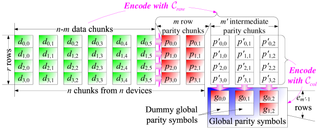
Figure 2: Exemplary configuration: a STAIR code stripe for $n=8$, $r=4$, $m=2$, and $\mathbf{e}=(1,1,2)$ (i.e., $m^{\prime}=3$ and $s=4$). Throughout this paper, we use this configuration to explain the operations of STAIR codes.

For general configuration parameters $n$, $r$, $m$, and $\mathbf{e}$, the main idea of STAIR encoding is to run two orthogonal encoding phases using two systematic MDS codes. First, we encode the data symbols using one code and obtain two types of parity symbols: row parity symbols, which protect against device failures, and intermediate parity symbols, which will then be encoded using another code to obtain global parity symbols, which protect against sector failures. In the following, we elaborate the encoding of STAIR codes and justify our naming convention.

We label different types of symbols for STAIR codes as follows. Figure 2 shows the layout of an exemplary stripe of a STAIR code for $n=8$, $r=4$, $m=2$, and $\mathbf{e}=(1,1,2)$ (i.e., $m^{\prime}=3$ and $s=4$). A stripe is composed of $n-m$ data chunks and $m$ row parity chunks. We also assume that there are $m^{\prime}$ intermediate parity chunks and $s$ global parity symbols outside the stripe. Let $d_{i,j}$, $p_{i,k}$, $p^{\prime}_{i,l}$, and $g_{h,l}$ denote a data symbol, a row parity symbol, an intermediate parity symbol, and a global parity symbol, respectively, where $0\leq i\leq r-1$, $0\leq j\leq n-m-1$, $0\leq k\leq m-1$, $0\leq l\leq m^{\prime}-1$, and $0\leq h\leq e_{l}-1$.

Figure 2 depicts the steps of the two orthogonal encoding phases of STAIR codes. In the first encoding phase, we use an $(n+m^{\prime},n-m)$-code denoted by $\mathcal{C}_{row}$ (which is an (11,6)-code in Figure 2). We encode via $\mathcal{C}_{row}$ each row of $n-m$ data symbols to obtain $m$ row parity symbols and $m^{\prime}$ intermediate parity symbols in the same row:

Phase 1: For $i=0,1,\cdots,r-1$,

$$d_{i,0},d_{i,1},\cdots,d_{i,n-m-1}\overset{\mathcal{C}_{row}}{\Longrightarrow}p_{i,0},p_{i,1},\cdots,p_{i,m-1},p^{\prime}_{i,0},p^{\prime}_{i,1},\cdots,p^{\prime}_{i,m^{\prime}-1},$$ (1)

where $\overset{\mathcal{C}}{\Longrightarrow}$ describes that the input symbols on the left are used to generate the output symbols on the right using some code $\mathcal{C}$. We call each $p_{i,k}$ a “row” parity symbol since it is only encoded from the same row of data symbols in the stripe, and we call each $p^{\prime}_{i,l}$ an “intermediate” parity symbol since it is not actually stored but is used in the second encoding phase only.

In the second encoding phase, we use a $(r+e_{m^{\prime}-1},r)$-code denoted by $\mathcal{C}_{col}$ (which is a (6,4)-code in Figure 2). We encode via $\mathcal{C}_{col}$ each chunk of $r$ intermediate parity symbols to obtain at most $e_{m^{\prime}-1}$ global parity symbols:

Phase 2: For $l=0,1,\cdots,m^{\prime}-1$,

$$p^{\prime}_{0,l},p^{\prime}_{1,l},\cdots,p^{\prime}_{r-1,l}\overset{\mathcal{C}_{col}}{\Longrightarrow}\overset{e_{m^{\prime}-1}}{\overbrace{g_{0,l},g_{1,l},\cdots,g_{e_{l}-1,l},*,\cdots,*}},$$ (2)

where “$*$” represents a “dummy” global parity symbol that will not be generated when $e_{l}<e_{m^{\prime}-1}$, and we only need to compute the “real” global parity symbols $g_{0,l},g_{1,l},\cdots,g_{e_{l}-1,l}$. The intermediate parity symbols will be discarded after this encoding phase. Note that each $g_{h,l}$ is in essence encoded from all the data symbols in the stripe, and thus we call it a “global” parity symbol.

We point out that $\mathcal{C}_{row}$ and $\mathcal{C}_{col}$ can be any systematic MDS codes. In this work, we implement both $\mathcal{C}_{row}$ and $\mathcal{C}_{col}$ using Cauchy Reed-Solomon codes [8, 38], which have no restriction on code length and fault tolerance.

From Figure 2, we see that the logical layout of global parity symbols looks like a stair. This is why we name this family of erasure codes STAIR codes.

In the following discussion, we use the exemplary configuration in Figure 2 to explain the detailed operations of STAIR codes. To simplify our discussion, we first assume that the global parity symbols are kept outside a stripe and are always available for ensuring fault tolerance. In §5, we will extend the encoding of STAIR codes when the global parity symbols are kept inside the stripe and are subject to both device and sector failures.

4 Upstairs Decoding

In this section, we justify the fault tolerance of STAIR codes defined by $m$ and $\mathbf{e}$. We introduce an upstairs decoding method that systematically recovers the lost symbols when both device and sector failures occur.

4.1 Homomorphic Property

The proof of fault tolerance of STAIR codes builds on the concept of a canonical stripe, which is constructed by augmenting the existing stripe with additional virtual parity symbols. To illustrate, Figure 3 depicts how we augment the stripe of Figure 2 into a canonical stripe. Let $d^{*}_{h,j}$ and $p^{*}_{h,k}$ denote the virtual parity symbols encoded with $\mathcal{C}_{col}$ from a data chunk and a row parity chunk, respectively, where $0\leq j\leq n-m-1$, $0\leq k\leq m-1$, and $0\leq h\leq e_{m^{\prime}-1}-1$. Specifically, we use $\mathcal{C}_{col}$ to generate virtual parity symbols from the data and row parity chunks as follows:

For $j=0,1,\cdots,n-m-1$,

$$d_{0,j},d_{1,j},\cdots,d_{r-1,j}\overset{\mathcal{C}_{col}}{\Longrightarrow}d^{*}_{0,j},d^{*}_{1,j},\cdots,d^{*}_{e_{m^{\prime}-1}-1,j};$$ (3)

and for $k=0,1,\cdots,m-1$,

$$p_{0,k},p_{1,k},\cdots,p_{r-1,k}\overset{\mathcal{C}_{col}}{\Longrightarrow}p^{*}_{0,k},p^{*}_{1,k},\cdots,p^{*}_{e_{m^{\prime}-1}-1,k}.$$ (4)

The virtual parity symbols $d^{*}_{h,j}$’s and $p^{*}_{h,k}$’s, along with the real and dummy global parity symbols, form $e_{m^{\prime}-1}$ augmented rows of $n+m^{\prime}$ symbols. In fact, the resulting canonical stripe in Figure 3 is a codeword of the product code [13] of $\mathcal{C}_{row}$ and $\mathcal{C}_{col}$. To make our discussion simpler, we number the rows and columns of the canonical stripe from 0 to $r+e_{m^{\prime}-1}-1$ and from 0 to $n+m^{\prime}-1$, respectively, as shown in Figure 3.

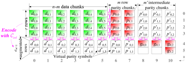
Figure 3: A canonical stripe augmented from the stripe in Figure 2. The rows and columns are labeled from 0 to 5 and 0 to 10, respectively, for ease of presentation.

Referring to Figure 3, we know that the upper $r$ rows of $n+m^{\prime}$ symbols are codewords of $\mathcal{C}_{row}$. We argue that each of the lower $e_{m^{\prime}-1}$ augmented rows is in fact also a codeword of $\mathcal{C}_{row}$. We call this the homomorphic property, since the encoding of each chunk in the column direction preserves the coding structure in the row direction. We formally prove the homomorphic property in Appendix A. We use this property to prove the fault tolerance of STAIR codes.

4.2 Proof of Fault Tolerance

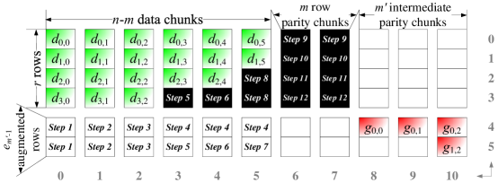
Figure 4: Upstairs decoding based on the canonical stripe in Figure 3.

We prove that for a STAIR code with configuration parameters $n$, $r$, $m$, and $\mathbf{e}$, as long as the failure pattern is within the failure coverage defined by $m$ and $\mathbf{e}$, the corresponding lost symbols can always be recovered (or decoded). In addition, we present an upstairs decoding method, which systematically recovers the lost symbols for STAIR codes.

For a stripe of the STAIR code, we consider the worst-case recoverable failure scenario where there are $m$ failed chunks (due to device failures) and $m^{\prime}$ additional chunks that have $e_{0}$, $e_{1}$, $\cdots$, $e_{m^{\prime}-1}$ lost symbols (due to sector failures), where $0<e_{0}\leq e_{1}\leq\cdots\leq e_{m^{\prime}-1}$. We prove that all the $m^{\prime}$ chunks with sector failures can be recovered with global parity symbols. In particular, we show that these $m^{\prime}$ chunks can be recovered in the order of $e_{0}$, $e_{1}$, $\cdots$, $e_{m^{\prime}-1}$. Finally, the $m$ failed chunks due to device failures can be recovered with row parity chunks.

4.2.1 Example

We demonstrate via our exemplary configuration how we recover the lost data due to both device and sector failures. Figure 4 shows the sequence of our decoding steps. Without loss of generality, we logically assign the column identities such that the $m^{\prime}$ chunks with sector failures are in Columns $n-m-m^{\prime}$ to $n-m-1$, with $e_{0}$, $e_{1}$, $\cdots$, $e_{m^{\prime}-1}$ lost symbols, respectively, and the $m$ failed chunks are in Columns $n-m$ to $n-1$. Also, the sector failures all occur in the bottom of the data chunks. Thus, the lost symbols form a stair, as shown in Figure 4.

The main idea of upstairs decoding is to recover the lost symbols from left to right and bottom to top. First, we see that there are $n-m-m^{\prime}=3$ good chunks (i.e., Columns 0-2) without any sector failure. We encode via $\mathcal{C}_{col}$ (which is a (6,4)-code) each such good chunk to obtain $e_{m^{\prime}-1}=2$ virtual parity symbols (Steps 1-3). In Row 4, there are now six available symbols. Thus, all the unavailable symbols in this row can be recovered using $\mathcal{C}_{row}$ (which is a (11,6)-code) due to the homomorphic property (Step 4). Note that we only need to recover the $m^{\prime}=3$ symbols that will later be used to recover sector failures. Column 3 (with $e_{0}=1$ sector failure) now has four available symbols. Thus, we can recover one lost symbol and one virtual parity symbol using $\mathcal{C}_{col}$ (Step 5). Similarly, we repeat the decoding for Column 4 (with $e_{1}=1$ sector failure) (Step 6). We see that Row 5 now contains six available symbols, so we can recover one unavailable virtual parity symbol (Step 7). Then Column 5 (with $e_{2}=2$ sector failures) now has four available symbols, so we can recover two lost symbols (Step 8). Now all chunks with sector failures are recovered. Finally, we recover the $m=2$ lost chunks row by row using $\mathcal{C}_{row}$ (Steps 9-12). Table 2 lists the detailed decoding steps of our example in Figure 4.

Table 2: Upstairs decoding: detailed steps for the example in Figure 4.

Step	Detailed Description			Coding Scheme
1	$d_{0,0},d_{1,0},d_{2,0},d_{3,0}$	$\Rightarrow$	$d^{*}_{0,0},d^{*}_{1,0}$	$\mathcal{C}_{col}$
2	$d_{0,1},d_{1,1},d_{2,1},d_{3,1}$	$\Rightarrow$	$d^{*}_{0,1},d^{*}_{1,1}$	$\mathcal{C}_{col}$
3	$d_{0,2},d_{1,2},d_{2,2},d_{3,2}$	$\Rightarrow$	$d^{*}_{0,2},d^{*}_{1,2}$	$\mathcal{C}_{col}$
4	$d^{*}_{0,0},d^{*}_{0,1},d^{*}_{0,2},g_{0,0},g_{0,1},g_{0,2}$	$\Rightarrow$	$d^{*}_{0,3},d^{*}_{0,4},d^{*}_{0,5}$	$\mathcal{C}_{row}$
5	$d_{0,3},d_{1,3},d_{2,3},d^{*}_{0,3}$	$\Rightarrow$	$d_{3,3},d^{*}_{1,3}$	$\mathcal{C}_{col}$
6	$d_{0,4},d_{1,4},d_{2,4},d^{*}_{0,4}$	$\Rightarrow$	$d_{3,4},d^{*}_{1,4}$	$\mathcal{C}_{col}$
7	$d^{*}_{1,0},d^{*}_{1,1},d^{*}_{1,2},d^{*}_{1,3},d^{*}_{1,4},g_{1,2}$	$\Rightarrow$	$d^{*}_{1,5}$	$\mathcal{C}_{row}$
8	$d_{0,5},d_{1,5},d^{*}_{0,5},d^{*}_{1,5}$	$\Rightarrow$	$d_{2,5},d_{3,5}$	$\mathcal{C}_{col}$
9	$d_{0,0},d_{0,1},d_{0,2},d_{0,3},d_{0,4},d_{0,5}$	$\Rightarrow$	$p_{0,1},p_{0,2}$	$\mathcal{C}_{row}$
10	$d_{1,0},d_{1,1},d_{1,2},d_{1,3},d_{1,4},d_{1,5}$	$\Rightarrow$	$p_{1,1},p_{1,2}$	$\mathcal{C}_{row}$
11	$d_{2,0},d_{2,1},d_{2,2},d_{2,3},d_{2,4},d_{2,5}$	$\Rightarrow$	$p_{2,1},p_{2,2}$	$\mathcal{C}_{row}$
12	$d_{3,0},d_{3,1},d_{3,2},d_{3,3},d_{3,4},d_{3,5}$	$\Rightarrow$	$p_{3,1},p_{3,2}$	$\mathcal{C}_{row}$

4.2.2 General Case

We now generalize the steps of upstairs decoding.

(1) Decoding of the chunk with $e_{0}$ sector failures: It is clear that there are $n-(m+m^{\prime})$ good chunks without any sector failure in the stripe. We use $\mathcal{C}_{col}$ to encode each such good chunk to obtain $e_{m^{\prime}-1}$ virtual parity symbols. Then each of the first $e_{0}$ augmented rows must now have $n-m$ available symbols: $n-(m+m^{\prime})$ virtual parity symbols that have just been encoded and $m^{\prime}$ global parity symbols. Since an augmented row is a codeword of $\mathcal{C}_{row}$ due to the homomorphic property, all the unavailable symbols in this row can be recovered using $\mathcal{C}_{row}$. Then, for the column with $e_{0}$ sector failures, it now has $r$ available symbols: $r-e_{0}$ good symbols and $e_{0}$ virtual parity symbols that have just been recovered. Thus, we can recover the $e_{0}$ sector failures as well as the $e_{m^{\prime}-1}-e_{0}$ unavailable virtual parity symbols using $\mathcal{C}_{col}$.

(2) Decoding of the chunk with $e_{i}$ sector failures ($1\leq i\leq m^{\prime}-1$): If $e_{i}=e_{i-1}$, we repeat the decoding for the chunk with $e_{i-1}$ sector failures. Otherwise, if $e_{i}>e_{i-1}$, each of the next $e_{i}-e_{i-1}$ augmented rows now has $n-m$ available symbols: $n-(m+m^{\prime})$ virtual parity symbols that are first recovered from the good chunks, $i$ virtual parity symbols that are recovered while the sector failures are recovered, and $m^{\prime}-i$ global parity symbols. Thus, all the unavailable virtual parity symbols in these $e_{i}-e_{i-1}$ augmented rows can be recovered. Then the column with $e_{i}$ sector failures now has $r$ available symbols: $r-e_{i}$ good symbols and $e_{i}$ virtual parity symbols that have been recovered. This column can then be recovered using $\mathcal{C}_{col}$. We repeat this process until all the $m^{\prime}$ chunks with sector failures are recovered.

(3) Decoding of the $m$ failed chunks: After all the $m^{\prime}$ chunks with sector failures are recovered, the $m$ failed chunks can be recovered row by row using $\mathcal{C}_{row}$.

4.3 Decoding in Practice

In §4.2, we describe an upstairs decoding method for the worst case. In practice, we often have fewer lost symbols than the worst case defined by $m$ and $\mathbf{e}$. To achieve efficient decoding, our idea is to recover as many lost symbols as possible via row parity symbols. The reason is that such decoding is local and involves only the symbols of the same row, while decoding via global parity symbols involves almost all data symbols within the stripe. In our implementation, we first locally recover any lost symbols using row parity symbols whenever possible. Then, for each chunk that still contains lost symbols, we count the number of its remaining lost symbols. Next, we globally recover the lost symbols with global parity symbols using upstairs decoding as described in §4.2, except those in the $m$ chunks that have the most lost symbols. These $m$ chunks can be finally recovered via row parity symbols after all other lost symbols have been recovered.

5 Extended Encoding: Relocating Global Parity Symbols Inside a Stripe

We thus far assume that there are always $s$ available global parity symbols that are kept outside a stripe. However, to maintain the regularity of the code structure and to avoid provisioning extra devices for keeping the global parity symbols, it is desirable to keep all global parity symbols inside a stripe. The idea is that in each stripe, we store the global parity symbols in some sectors that originally store the data symbols. A challenge is that such inside global parity symbols are also subject to both device and sector failures, so we must maintain their fault tolerance during encoding. In this section, we propose two encoding methods, namely upstairs encoding and downstairs encoding, which support the construction of inside global parity symbols, while preserving the homomorphic property and hence the fault tolerance of STAIR codes. These two encoding methods produce the same values for parity symbols, but differ in computational complexities for different configurations. We show how to deduce parity relations from the two encoding methods, and also show that the two encoding methods have complementary performance advantages for different configurations.

5.1 Two New Encoding Methods

5.1.1 Upstairs Encoding

We let $\hat{g}_{h,l}$ ($0\leq l\leq m^{\prime}-1$ and $0\leq h\leq e_{l}-1$) be an inside global parity symbol. Figure 5 illustrates how we place the inside global parity symbols. Without loss of generality, we place them at the bottom of the rightmost data chunks, following the stair layout. Specifically, we choose the $m^{\prime}=3$ rightmost data chunks in Columns 3-5 and place $e_{0}=1$, $e_{1}=1$, and $e_{2}=2$ global parity symbols at the bottom of these data chunks, respectively. That is, the original data symbols $d_{3,3}$, $d_{3,4}$, $d_{2,5}$, and $d_{3,5}$ are now replaced by the inside global parity symbols $\hat{g}_{0,0}$, $\hat{g}_{0,1}$, $\hat{g}_{0,2}$, and $\hat{g}_{1,2}$, respectively.

Figure 5: Upstairs encoding: we set outside global parity symbols to be zero and reconstruct the inside global parity symbols using upstairs decoding (see §4.2).

Figure 6: Downstairs encoding: we compute the parity symbols from top to bottom and right to left.

To obtain the inside global parity symbols, we extend the upstairs decoding method in §4.2 and propose a recovery-based encoding approach called upstairs encoding. We first set all the outside global parity symbols to be zero (see Figure 5). Then we treat all $m=2$ row parity chunks and all $s=4$ inside global parity symbols as lost chunks and lost sectors, respectively. Now we “recover” all inside global parity symbols, followed by the $m=2$ row parity chunks, using the upstairs decoding method in §4.2. Since all outside global parity symbols are set to be zero, we need not store them. The homomorphic property, and hence the fault tolerance property, remain the same as discussed in §4. Thus, in failure mode, we can still use upstairs decoding to reconstruct lost symbols. We call this encoding method “upstairs encoding” because the parity symbols are encoded from bottom to top as described in §4.2.

5.1.2 Downstairs Encoding

In addition to upstairs encoding, we present a different encoding method called downstairs encoding, in which we generate parity symbols from top to bottom and right to left. We illustrate the idea in Figure 6, which depicts the sequence of generating parity symbols. We still set the outside global parity symbols to be zero. First, we encode via $\mathcal{C}_{row}$ the $n-m=6$ data symbols in each of the first $r-e_{m^{\prime}-1}=2$ rows (i.e., Rows 0 and 1) and generate $m+m^{\prime}=5$ parity symbols (including two row parity symbols and three intermediate parity symbols) (Steps 1-2). The rightmost column (i.e., Column 10) now has $r=4$ available symbols, including the two intermediate parity symbols that are just encoded and two zeroed outside global parity symbols. Thus, we can recover $e_{m^{\prime}-1}=2$ intermediate parity symbols using $\mathcal{C}_{col}$ (Step 3). We can generate $m+m^{\prime}=5$ parity symbols (including one inside global parity symbol, two row parity symbols, and two intermediate parity symbols) for Row 2 using $\mathcal{C}_{row}$ (Step 4), followed by $e_{m^{\prime}-2}=1$ and $e_{m^{\prime}-3}=1$ intermediate parity symbols in Columns 9 and 8 using $\mathcal{C}_{col}$, respectively (Steps 5-6). Finally, we obtain the remaining $m+m^{\prime}=5$ parity symbols (including three global parity symbols and two row parity symbols) for Row 3 using $\mathcal{C}_{row}$ (Step 7). Table 3 shows the detailed steps of downstairs encoding for the example in Figure 6.

Table 3: Downstairs decoding: detailed steps for the example in Figure 6.

Step	Detailed Description			Coding Scheme
1	$d_{0,0},d_{0,1},d_{0,2},d_{0,3},d_{0,4},d_{0,5}$	$\Rightarrow$	$p_{0,0},p_{0,1},p^{\prime}_{0,0},p^{\prime}_{0,1},p^{\prime}_{0,2}$	$\mathcal{C}_{row}$
2	$d_{1,0},d_{1,1},d_{1,2},d_{1,3},d_{1,4},d_{1,5}$	$\Rightarrow$	$p_{1,0},p_{1,1},p^{\prime}_{1,0},p^{\prime}_{1,1},p^{\prime}_{1,2}$	$\mathcal{C}_{row}$
3	$p^{\prime}_{0,2},p^{\prime}_{1,2},g_{0,2}=0,g_{1,2}=0$	$\Rightarrow$	$p^{\prime}_{2,2},p^{\prime}_{3,2}$	$\mathcal{C}_{col}$
4	$d_{2,0},d_{2,1},d_{2,2},d_{2,3},d_{2,4},p^{\prime}_{2,2}$	$\Rightarrow$	$\hat{g}_{0,2},p_{2,0},p_{2,1},p^{\prime}_{2,0},p^{\prime}_{2,1}$	$\mathcal{C}_{row}$
5	$p^{\prime}_{0,1},p^{\prime}_{1,1},p^{\prime}_{2,1},g_{0,1}=0$	$\Rightarrow$	$p^{\prime}_{3,1}$	$\mathcal{C}_{col}$
6	$p^{\prime}_{0,0},p^{\prime}_{1,0},p^{\prime}_{2,0},g_{0,0}=0$	$\Rightarrow$	$p^{\prime}_{3,0}$	$\mathcal{C}_{col}$
7	$d_{3,0},d_{3,1},d_{3,2},p^{\prime}_{3,0},p^{\prime}_{3,1},p^{\prime}_{3,2}$	$\Rightarrow$	$\hat{g}_{0,0},\hat{g}_{0,1},\hat{g}_{1,2},p_{3,0},p_{3,1}$	$\mathcal{C}_{row}$

In general, we start with encoding via $\mathcal{C}_{row}$ the rows from top to bottom. In each row, we generate $m+m^{\prime}$ symbols. When no more rows can be encoded because of insufficient available symbols, we encode via $\mathcal{C}_{col}$ the columns from right to left to obtain new intermediate parity symbols (initially, we obtain $e_{m^{\prime}-1}$ symbols, followed by $e_{m^{\prime}-2}$ symbols, and so on). We alternately encode rows and columns until all parity symbols are formed. We can generalize the steps as in §4.2.2, but we omit the details in the interest of space.

It is important to note that the downstairs encoding method cannot be generalized for decoding lost symbols. For example, referring to our exemplary configuration, we consider a worst-case recoverable failure scenario in which both row parity chunks are entirely failed, and the data symbols $d_{0,3}$, $d_{1,4}$, $d_{2,2}$, and $d_{3,2}$ are lost. In this case, we cannot recover the lost symbols in the top row first, but instead we must resort to upstairs decoding as described in §4.2. Upstairs decoding works because we limit the maximum number of chunks with lost symbols (i.e., at most $m+m^{\prime}$). This enables us to first recover the leftmost virtual parity symbols of the augmented rows first and gradually reconstruct lost symbols. On the other hand, we do not limit the number of rows with lost symbols in our configuration, so the downstairs method cannot be used for general decoding.

5.1.3 Discussion

Note that both upstairs and downstairs encoding methods always generate the same values for all parity symbols, since both of them preserve the homomorphic property, fix the outside global parity symbols to be zero, and use the same schemes $\mathcal{C}_{row}$ and $\mathcal{C}_{col}$ for encoding.

Also, both of them reuse parity symbols in the intermediate steps to generate additional parity symbols in subsequent steps. On the other hand, they differ in encoding complexity, due to the different ways of reusing the parity symbols. We analyze this in §5.3.

5.2 Uneven Parity Relations

Before relocating the global parity symbols inside a stripe, each data symbol contributes to $m$ row parity symbols and all $s$ outside global parity symbols. However, after relocation, the parity relations become uneven. That is, some row parity symbols are also contributed by the data symbols in other rows, while some inside global parity symbols are contributed by only a subset of data symbols in the stripe. Here, we discuss the uneven parity relations of STAIR codes so as to better understand the encoding and update performance of STAIR codes in subsequent analysis.

Figure 7: A stair step with a tread and a riser.

To analyze how exactly each parity symbol is generated, we revisit both upstairs and downstairs encoding methods. Recall that the row parity symbols and the inside global parity symbols are arranged in the form of stair steps, each of which is composed of a tread (i.e., the horizontal portion of a step) and a riser (i.e., the vertical portion of a step), as shown in Figure 7. If upstairs encoding is used, then from Figure 4, the encoding of each parity symbol does not involve any data symbol on its right. Also, among the columns spanned by the same tread, the encoding of parity symbols in each column does not involve any data symbol in other columns. We can make similar arguments for downstairs encoding. If downstairs encoding is used, then from Figure 6, the encoding of each parity symbol does not involve any data symbol below it. Also, among the rows spanned by the same riser, the encoding of parity symbols in each row does not involve any data symbol in other rows.

Figure 8: The data symbols that contribute to parity symbols $p_{2,0}$, $\hat{g}_{0,1}$, and $p_{1,1}$, respectively.

As both upstairs and downstairs encoding methods generate the same values of parity symbols, we can combine the above arguments into the following property of how each parity symbol is related to data symbols.

Property 5.1

(Parity relations in STAIR codes): In a STAIR code stripe, a (row or inside global) parity symbol in Row $i_{0}$ and Column $j_{0}$ (where $0\leq i_{0}\leq r-1$ and $n-m-m^{\prime}\leq j_{0}\leq n-1$) depends only on the data symbols $d_{i,j}$’s where $i\leq i_{0}$ and $j\leq j_{0}$. Moreover, each parity symbol is unrelated to any data symbol in any other column (row) spanned by the same tread (riser).

Figure 8 illustrates the above property. For example, $p_{2,0}$ depends only on the data symbols $d_{i,j}$’s in Rows 0-2 and Columns 0-5. Note that $\hat{g}_{0,1}$ in Column 4 is unrelated to any data symbol in Column 3, which is spanned by the same tread as Column 4. Similarly, $p_{1,1}$ in Row 1 is unrelated to any data symbol in Row 0, which is spanned by the same riser as Row 1.

5.3 Encoding Complexity Analysis

Figure 9: Numbers of Mult_XORs (per stripe) of the three encoding methods for STAIR codes versus different $\mathbf{e}$’s when $n=8$, $m=2$, and $s=4$.

We have proposed two encoding methods for STAIR codes: upstairs encoding and downstairs encoding. Both of them alternately encode rows and columns to obtain the parity symbols. We can also obtain parity symbols using the standard encoding approach, in which each parity symbol is computed directly from a linear combination of data symbols as in classical Reed-Solomon codes. We now analyze the computational complexities of these three methods for different configuration parameters of STAIR codes.

STAIR codes perform encoding over a Galois Field, in which linear arithmetic can be decomposed into the basic operations Mult_XORs [36]. We define $\mbox{{Mult\_XOR}}(\mathbf{R}_{1},\mathbf{R}_{2},a)$ as an operation that first multiplies a region $\mathbf{R}_{1}$ of bytes by a $w$-bit constant $a$ in Galois Field $GF(2^{w})$, and then applies XOR-summing to the product and the target region $\mathbf{R}_{2}$ of the same size. For example, $\mathbf{Y}=a_{0}\cdot\mathbf{X}_{0}+a_{1}\cdot\mathbf{X}_{1}$ can be decomposed into two Mult_XORs (assuming $\mathbf{Y}$ is initialized as zero): $\mbox{{Mult\_XOR}}(\mathbf{X}_{0},\mathbf{Y},a_{0})$ and $\mbox{{Mult\_XOR}}(\mathbf{X}_{1},\mathbf{Y},a_{1})$. Clearly, fewer Mult_XORs imply a lower computational complexity. To evaluate the computational complexity of an encoding method, we count its number of Mult_XORs (per stripe).

For upstairs encoding, we generate $m\cdot r$ row parity symbols and $s$ virtual parity symbols along the row direction, as well as $s$ inside global parity symbols and $(n-m)\cdot e_{m^{\prime}-1}-s$ virtual parity symbols along the column direction. Its number of Mult_XORs (denoted by $\mathcal{X}_{up}$) is:

$$\mathcal{X}_{up}=\overset{\footnotesize\mbox{row direction}}{\overbrace{(n-m)\times(m\cdot r+s)}}+\overset{\footnotesize\mbox{column direction}}{\overbrace{r\times\left[(n-m)\cdot e_{m^{\prime}-1}\right]}}.$$ (5)

For downstairs encoding, we generate $m\cdot r$ row parity symbols, $s$ inside global parity symbols, and $m^{\prime}\cdot r-s$ intermediate parity symbols along the row direction, as well as $s$ intermediate parity symbols along the column direction. Its number of Mult_XORs (denoted by $\mathcal{X}_{down}$) is:

$$\mathcal{X}_{down}=\overset{\footnotesize\mbox{row direction}}{\overbrace{(n-m)\times\left[(m+m^{\prime})\cdot r\right]}}+\overset{\footnotesize\mbox{column direction}}{\overbrace{r\times s}}.$$ (6)

For standard encoding, we compute the number of Mult_XORs by summing the number of data symbols that contribute to each parity symbol, based on the property of uneven parity relations discussed in §5.2.

We show via a case study how the three encoding methods differ in the number of Mult_XORs. Figure 9 depicts the numbers of Mult_XORs of the three encoding methods for different $\mathbf{e}$’s in the case where $n=8$, $m=2$, and $s=4$. Upstairs encoding and downstairs encoding incur significantly fewer Mult_XORs than standard encoding most of the time. The main reason is that both upstairs encoding and downstairs encoding often reuse the computed parity symbols in subsequent encoding steps. We also observe that for a given $s$, the number of Mult_XORs of upstairs encoding increases with $e_{m^{\prime}-1}$ (see Equation (5)), while that of downstairs encoding increases with $m^{\prime}$ (see Equation (6)). Since larger $m^{\prime}$ often implies smaller $e_{m^{\prime}-1}$, the value of $m^{\prime}$ often determines which of the two encoding methods is more efficient: when $m^{\prime}$ is small, downstairs encoding wins; when $m^{\prime}$ is large, upstairs encoding wins.

In our encoding implementation of STAIR codes, for given configuration parameters, we always pre-compute the number of Mult_XORs for each of the encoding methods, and then choose the one with the fewest Mult_XORs.

6 Storage and Performance Evaluation

Figure 10: Space saving of STAIR codes over traditional erasure codes in terms of $s$, $m^{\prime}$, and $r$.

We evaluate STAIR codes and compare them with other related erasure codes in different practical aspects, including storage space saving, encoding/decoding speed, and update penalty.

6.1 Storage Space Saving

The main motivation for STAIR codes is to tolerate simultaneous device and sector failures with significantly lower storage space overhead than traditional erasure codes (e.g., Reed-Solomon codes) that provide only device-level fault tolerance. Given a failure scenario defined by $m$ and $\mathbf{e}$, traditional erasure codes need $m+m^{\prime}$ chunks per stripe for parity, while STAIR codes need only $m$ chunks and $s$ symbols (where $m^{\prime}\leq s$). Thus, STAIR codes save $r\times m^{\prime}-s$ symbols per stripe, or equivalently, $m^{\prime}-\frac{s}{r}$ devices per system. In short, the saving of STAIR codes depends on only three parameters $s$, $m^{\prime}$, and $r$ (where $s$ and $m^{\prime}$ are determined by $\mathbf{e}$).

Figure 10 plots the number of devices saved by STAIR codes for $s\leq 4$, $m^{\prime}\leq s$, and $r\leq 32$. As $r$ increases, the number of devices saved is close to $m^{\prime}$. The saving reaches the highest when $m^{\prime}=s$.

We point out that the recently proposed SD codes [33, 32] are also motivated for reducing the storage space over traditional erasure codes. Unlike STAIR codes, SD codes always achieve a saving of $s-\frac{s}{r}$ devices, which is the maximum saving of STAIR codes. While STAIR codes apparently cannot outperform SD codes in space saving, it is important to note that the currently known constructions of SD codes are limited to $s\leq 3$ only [33, 32, 7], implying that SD codes can save no more than three devices. On the other hand, STAIR codes do not have such limitations. As shown in Figure 10, STAIR codes can save more than three devices for larger $s$.

6.2 Encoding/Decoding Speed

We evaluate the encoding/decoding speed of STAIR codes. Our implementation of STAIR codes is written in C. We leverage the GF-Complete open source library [36] to accelerate Galois Field arithmetic using Intel SIMD instructions. Our experiments compare STAIR codes with the state-of-the-art SD codes [33, 32]. At the time of this writing, the open-source implementation of SD codes encodes stripes in a decoding manner without any parity reuse. For fair comparisons, we extend the SD code implementation to support the standard encoding method mentioned in §5.3. We run our performance tests on a machine equipped with an Intel Core i5-3570 CPU at 3.40GHz with SSE4.2 support. The CPU has a 256KB L2-cache and a 6MB L3-cache.

6.2.1 Encoding

We compare the encoding performance of STAIR codes and SD codes for different values of $n$, $r$, $m$, and $s$. For SD codes, we only consider the range of configuration parameters where $s\leq 3$, since no code construction is available outside this range [33, 32, 7]. In addition, the SD code constructions for $s=3$ are only available in the range $n\leq 24$, $r\leq 24$, and $m\leq 3$ [33, 32]. For STAIR codes, a single value of $s$ can imply different configurations of $\mathbf{e}$ (e.g., see Figure 9 in §5.3), each of which has different encoding performance. Here, we take a conservative approach to analyze the worst-case performance of STAIR codes, that is, we test all possible configurations of $\mathbf{e}$ for a given $s$ and pick the one with the lowest encoding speed.

Note that the encoding performance of both STAIR codes and SD codes heavily depends on the word size $w$ of the adopted Galois Field $GF(2^{w})$, where $w$ is often set to be a power of 2. A smaller $w$ often means a higher encoding speed [36]. STAIR codes work as long as $n+m^{\prime}\leq 2^{w}$ and $r+e_{m^{\prime}-1}\leq 2^{w}$. Thus, we choose $w=8$ since it suffices for all of our tests. However, SD codes may choose among $w=8$, $w=16$, and $w=32$, depending on configuration parameters. We choose the smallest $w$ that is feasible for the SD code construction.

We consider the metric encoding speed, defined as the amount of data encoded per second. We construct a stripe of size roughly 32MB in memory [33, 32]. We put random bytes in the stripe, and divide the stripe into $r\times n$ sectors, each mapped to a symbol. We obtain the averaged results over 10 runs.

(a) Varying $n$ when $r=16$

(b) Varying $r$ when $n=16$

Figure 11: Encoding speed of STAIR codes and SD codes for different combinations of $n$, $r$, $m$, and $s$.

Figure 12: Encoding speed of STAIR codes and SD codes for different stripe sizes when $n=16$ and $r=16$.

Figures 11(a) and 11(b) present the encoding speed results for different values of $n$ when $r=16$ and for different values of $r$ when $n=16$, respectively. In most cases, the encoding speed of STAIR codes is over 1000MB/s, which is significantly higher than the disk write speed in practice (note that although disk writes can be parallelized in disk arrays, the encoding operations can also be parallelized with modern multi-core CPUs). The speed increases with both $n$ and $r$. The intuitive reason is that the proportion of parity symbols decreases with $n$ and $r$. Compared to SD codes, STAIR codes improve the encoding speed by $106.03\%$ on average (in the range from $29.30\%$ to $225.14\%$). The reason is that STAIR codes reuse encoded parity information in subsequent encoding steps by upstairs/downstairs encoding (see §5.3), while such an encoding property is not exploited in SD codes.

We also evaluate the impact of stripe size on the encoding speed of STAIR codes and SD codes for given $n$ and $r$. We fix $n=16$ and $r=16$, and vary the stripe size from 128KB to 512MB. Note that a stripe of size 128KB implies a symbol of size 512 bytes, the standard sector size in practical disk drives. Figure 12 presents the encoding speed results. As the stripe size increases, the encoding speed of both STAIR codes and SD codes first increases and then drops, due to the mixed effects of SIMD instructions adopted in GF-Complete [36] and CPU cache. Nevertheless, the encoding speed advantage of STAIR codes over SD codes remains unchanged.

6.2.2 Decoding

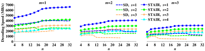
(a) Varying $n$ when $r=16$

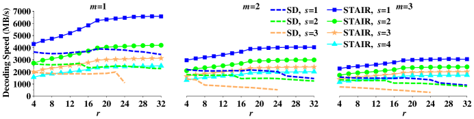
(b) Varying $r$ when $n=16$

Figure 13: Decoding speed of STAIR codes and SD codes for different combinations of $n$, $r$, $m$, and $s$.

We measure the decoding performance of STAIR codes and SD codes in recovering lost symbols. Since the decoding time increases with the number of lost symbols to be recovered, we consider a particular worst case in which the $m$ leftmost chunks and $s$ additional symbols in the following $m^{\prime}$ chunks defined by $\mathbf{e}$ are all lost. The evaluation setup is similar to that in §6.2.1, and in particular, the stripe size is fixed at 32MB.

Figures 13(a) and 13(b) present the decoding speed results for different $n$ when $r=16$ and for different $r$ when $n=16$, respectively. The results of both figures can be viewed in comparison to those of Figures 11(a) and 11(b), respectively. Similar to encoding, the decoding speed of STAIR codes is over 1000MB/s in most cases and increases with both $n$ and $r$. Compared to SD codes, STAIR codes improve the decoding speed by $102.99\%$ on average (in the range from $1.70\%$ to $537.87\%$).

In practice, we often have fewer lost symbols than the worst case (see §4.3). One common case is that there are only failed chunks due to device failures (i.e., $s=0$), so the decoding of both STAIR and SD codes is identical to that of Reed-Solomon codes. In this case, the decoding speed of STAIR/SD codes can be significantly higher than that of $s=1$ for STAIR codes in Figure 13. For example, when $n=16$ and $r=16$, the decoding speed increases by 79.39%, 29.39%, and 11.98% for $m=1$, $2$, and $3$, respectively.

6.3 Update Penalty

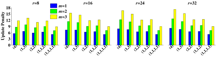
Figure 14: Update penalty of STAIR codes for different $\mathbf{e}$’s when $n=16$ and $s=4$.

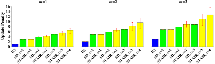
Figure 15: Update penalty of STAIR codes, SD codes, and Reed-Solomon (RS) codes when $n=16$ and $r=16$. For STAIR codes, we plot the error bars for the maximum and minimum update penalty values among all possible configurations of $\mathbf{e}$.

We evaluate the update cost of STAIR codes when data symbols are updated. For each data symbol in a stripe being updated, we count the number of parity symbols being affected (see §5.2). Here, we define the update penalty as the average number of parity symbols that need to be updated when a data symbol is updated.

Clearly, the update penalty of STAIR codes increases with $m$. We are more interested in how $\mathbf{e}$ influences the update penalty of STAIR codes. Figure 14 presents the update penalty results for different $\mathbf{e}$’s when $n=16$ and $s=4$. For different $\mathbf{e}$’s with the same $s$, the update penalty of STAIR codes often increases with $e_{m^{\prime}-1}$. Intuitively, a larger $e_{m^{\prime}-1}$ implies that more rows of row parity symbols are encoded from inside global parity symbols, which are further encoded from almost all data symbols (see §5.2).

We compare STAIR codes with SD codes [33, 32]. For STAIR codes with a given $s$, we test all possible configurations of $\mathbf{e}$ and find the average, minimum, and maximum update penalty. For SD codes, we only consider $s$ between 1 and 3. We also include the update penalty results of Reed-Solomon codes for reference. Figure 15 presents the update penalty results when $n=16$ and $r=16$ (while similar observations are made for other $n$ and $r$). For a given $s$, the range of update penalty of STAIR codes covers that of SD codes, although the average is sometimes higher than that of SD codes (same for $s=1$, by 7.30% to 14.02% for $s=2$, and by 10.47% to 23.72% for $s=3$). Both STAIR codes and SD codes have higher update penalty than Reed-Solomon codes due to more parity symbols in a stripe, and hence are suitable for storage systems with rare updates (e.g., backup or write-once-read-many (WORM) systems) or systems dominated by full-stripe writes [33, 32].

7 Reliability Analysis

In the previous section, we examine the storage and performance properties of STAIR codes. We now characterize the reliability of STAIR codes using analytical models. We also show that STAIR codes effectively tolerate sector failure bursts [1, 41] by supporting a wide range of configurations of the sector failure coverage defined by $\mathbf{e}$. We extend the reliability analysis by Dholakia et al. [11] specifically for STAIR codes, whose fault tolerance is defined by the specific configuration of $\mathbf{e}$. Table 4 summarizes the major notation for our reliability analysis.

Table 4: Major notation used for reliability analysis.

Notation	Description
$U$	Total amount (in bytes) of user data stored in a storage system
$C$	Device capacity (in bytes)
$S$	Sector size (in bytes)
$E$	Storage efficiency of an erasure code
$N_{arr}$	Number of storage arrays in a storage system
$MTTDL_{sys}$	MTTDL of a storage system
${MTTDL}_{arr}$	MTTDL of a single storage array
$1/\lambda$	Mean time to device failure
$1/\mu$	Mean time to rebuild in critical mode
$P_{arr}$	Probability that a storage array in critical mode encounters unrecoverable sector failures in non-failed devices
$P_{str}$	Probability that a stripe in critical mode encounters unrecoverable sector failures in non-failed chunks
$P_{chk(i)}$	Probability that a chunk encounters $i$ sector failures (where $0\leq i\leq r$)
$P_{bit}$	Probability of an unrecoverable bit error
$P_{sec}$	Probability of a sector failure
$B$	Average length (in number of sectors) of a sector failure burst
$b_{i}$	Fraction of sector failure bursts of length $i$ (where $i\geq 1$)
$\alpha$	Tail index of a Pareto distribution that best fits the distribution of length $\geq 2$ for sector failure bursts

7.1 Analytical Models

In this subsection, we develop analytical models for the reliability analysis.

7.1.1 MTTDL Model

We first model the overall reliability of a storage system. We use the standard reliability metric called mean time to data loss (MTTDL), although other advanced metrics have been proposed in the literature [16].

Recall from §2 that we encode a storage array using a STAIR code with configuration parameters $n$, $r$, $m$, and $\mathbf{e}$ (and hence $s$). Consider a storage system with $N_{arr}$ storage arrays, each with $n$ devices of capacity $C$. To store a given amount $U$ of user data, $N_{arr}$ should be set to be:

$$N_{arr}=\left\lceil\frac{\left.U\middle/E\right.}{C\cdot n}\right\rceil,$$ (7)

where $E$ denotes the storage efficiency of an erasure code (i.e., the fraction of storage capacity used for storing the actual data). For STAIR codes, $E$ can be calculated by:

$$E=\frac{r\cdot(n-m)-s}{r\cdot n}\times 100\%.$$ (8)

Note that the storage efficiency of Reed-Solomon codes can be obtained from Equation (8) by setting $s=0$, while that of an SD code with a given $s$ [33, 32] can be directly computed via Equation (8).

Let $MTTDL_{arr}$ be the MTTDL of a storage array. Suppose that $MTTDL_{arr}$ is exponentially distributed. Then the MTTDL of the whole storage system (denoted by $MTTDL_{sys}$) can be calculated by:

$$MTTDL_{sys}=\frac{MTTDL_{arr}}{N_{arr}}.$$ (9)

Figure 16: Markov model for a storage array with $m=1$: State 0 means no device failure; State 1 means one device failure; and State DL means data loss.

We first derive $MTTDL_{arr}$ as in the work [11]. To simplify our analysis, we only consider the most practical case where $m=1$. When a storage array experiences a device failure, it enters critical mode, in which either an additional device failure or an unrecoverable sector failure in a non-failed device can lead to data loss. For device failures, suppose that they are independent and exponentially distributed with parameter $\lambda$, where $1/\lambda$ is the mean time to device failure; for sector failures, suppose that the probability that a storage array in critical mode encounters unrecoverable sector failures in non-failed devices is $P_{arr}$. In addition, suppose that the rebuild time in critical mode is exponentially distributed with parameter $\mu$, where $1/\mu$ is the mean time to rebuild. Figure 16 depicts the corresponding Markov model [11], where State 0 means no device failure, State 1 means one device failure, and State DL means data loss. In this Markov model, we do not consider the scenario where a storage array in State 0 encounters a sector failure, by assuming that the storage array can recover the sector failure in a very short time ($\ll 1/\mu$) and is highly unlikely to encounter another device or sector failure that may lead to data loss. An explicit expression of $MTTDL_{arr}$ deduced based on this Markov model can be derived as follows [11]:

$$MTTDL_{arr}=\frac{(2n-1)\lambda+\mu}{n\lambda[(n-1)\lambda+\mu P_{arr}]}.$$ (10)

We next derive $P_{arr}$. Recall that each stripe is independently encoded in a storage array (see §2). Let $P_{str}$ be the probability that a stripe in critical mode encounters unrecoverable sector failures in non-failed chunks. Since the number of stripes in a storage array is $\left\lfloor\frac{C}{S\cdot r}\right\rfloor$, where $S$ is the sector size in bytes (typically 512 bytes), we have

$$P_{arr}=1-(1-P_{str})^{\left\lfloor\frac{C}{S\cdot r}\right\rfloor}\approx\left\lfloor\frac{C}{S\cdot r}\right\rfloor\cdot P_{str}.$$ (11)

Finally, we discuss how to derive $P_{str}$. In critical mode, there are $n-m$ non-failed chunks in a stripe. Suppose that each non-failed chunk independently suffers from sector failures. Let $P_{chk(i)}$ (where $0\leq i\leq r$) be the probability that a non-failed chunk encounters $i$ sector failures. For the STAIR code with a given $\mathbf{e}$, we compute $P_{str}$ as a function of $P_{chk(i)}$’s by enumerating all cases of sector failures. For example, if $\mathbf{e}=(s)$ (where $s\geq 1$), then $P_{str}$ can be computed by the complement of the probability that all $n-m$ non-failed chunks have no sector failure or exactly one non-failed chunk has one up to $s$ sector failures. Appendix B describes the explicit expressions of $P_{str}$ for some specific configurations of $\mathbf{e}$ considered in our analysis. For comparisons, Appendix B also describes the explicit expressions of $P_{str}$ for Reed-Solomon codes and SD codes. Note that the values of $P_{chk(i)}$’s are determined by the sector failure model, which we describe below.

7.1.2 Sector Failure Models

Let $P_{sec}$ be the probability of a sector failure, and $P_{bit}$ be the probability of an unrecoverable bit error. Suppose that bit errors are independent. Then $P_{sec}$ can be estimated by:

$$P_{sec}=1-(1-{P}_{bit})^{S\times 8}\approx(S\times 8)\cdot{P}_{bit}.$$ (12)

We now consider two models for sector failures [11]: the independent model and the correlated model. We fix $P_{sec}$ in both models, so both models see the same expected number of sector failures in the whole array. Intuitively, in the independent model, we assume that sector failures occur independently, so sector failures tend to be scattered across different chunks within a stripe. In the correlated model, we assume that sector failures come in bursts, according to the previous field studies [1, 41]. Thus, sector failures tend to appear together in one of the chunks within a stripe. We derive $P_{chk(i)}$ (where $0\leq i\leq r$) for each model as follows.

In the independent model, $P_{chk(i)}$ (where $0\leq i\leq r$) is calculated by:

$$P_{chk(i)}={r\choose i}\cdot P_{sec}^{i}\cdot(1-P_{sec})^{r-i}.$$ (13)

In the correlated model, let $B$ be the average length (in number of sectors) of a sector failure burst. While the burst length may vary across different bursts, it is shown that the average length $B$ is close to one sector (e.g., $B=1.0291$ [11]). To simplify our analysis, we assume that the burst length is at most $r$ sectors in all cases, and that a burst spans one chunk only (i.e., it does not span across two chunks). We further assume that sector failure bursts are independent of each other. Let $b_{i}$ be the fraction of sector failure bursts of length $i$ (where $1\leq i\leq r$) in a storage array (note that $\sum_{i=1}^{r}{b_{i}}=1$). Then, we have:

$$B=\sum_{i=1}^{r}{i\times b_{i}}.$$ (14)

Note that the probability that a sector is the beginning of a sector failure burst is given by $P_{sec}\cdot\frac{1}{B}$. Moreover, $P_{chk(0)}$ is equal to the probability that each of the $r$ sectors in a chunk is not the beginning of a sector failure burst. Thus, we have:

$$P_{chk(0)}=(1-\frac{P_{sec}}{B})^{r}\approx 1-r\cdot\frac{P_{sec}}{B}.$$ (15)

In other words, the probability that a chunk encounters at least one sector failure is:

$$P_{chk(1)}+P_{chk(2)}+\cdots+P_{chk(r)}=1-P_{chk(0)}\approx r\cdot\frac{P_{sec}}{B}.$$ (16)

We can compute $P_{chk(i)}$ (where $1\leq i\leq r$) as:

$$P_{chk(i)}=b_{i}\cdot\left(r\cdot\frac{P_{sec}}{B}\right).$$ (17)

7.2 Numerical Results

We examine the system reliability $MTTDL_{sys}$ of STAIR codes and compare it with those of Reed-Solomon codes and SD codes. We follow the storage array configurations in the work [11]. We consider a storage system that stores $U=10$PB of user data using SATA disk drives with parameters $C=300$GB, $S=512$ bytes, $1/\lambda=500,000$ hours, and $1/\mu=17.8$ hours. In each storage array, we fix $n=8$, $r=16$, and $m=1$. We consider different values of $s$ (note that $s=0$ corresponds to Reed-Solomon codes). For a given $s$, to store 10PB of user data, we set the number $N_{arr}$ of storage arrays as follows:

$s$	0	1	2	3	4	5	6
$N_{arr}$	4994	5039	5085	5131	5179	5227	5276
$s$	7	8	9	10	11	12
$N_{arr}$	5327	5378	5430	5483	5538	5593

For the probability $P_{bit}$ of an unrecoverable bit error in SATA disk drives, we pick the range $[10^{-14},10^{-10}]$ to cover the data sheet value $10^{-14}$ considered by Dholakia et al. [11] and the empirical values that are much higher than stated in data sheets [24]. We investigate how $P_{bit}$ affects the system reliability.

7.2.1 Independent Sector Failures

(a) STAIR/SD codes with $s\leq 2$ and RS codes

(b) STAIR codes with $s=3$

Figure 17: $MTTDL_{sys}$ results of STAIR codes, SD codes, and Reed-Solomon (RS) codes for different $P_{bit}$’s in the independent sector failure model.

We first consider the case of independent sector failures. Figure 17 depicts $MTTDL_{sys}$ results of different erasure codes versus $P_{bit}$. From Figure 17(a), we observe that both the STAIR code and SD code with $s=1$ achieve much higher reliability than Reed-Solomon codes, for example, by more than two orders of magnitude at $P_{bit}=10^{-14}$. As $P_{bit}$ increases, the reliability of Reed-Solomon codes follows a power-law decrease, while those of the STAIR code and SD code with $s=1$ remain almost unchanged. The reason is that both STAIR codes and SD codes can protect against the data loss due to an additional sector failure with an additional parity sector. As $P_{bit}$ further increases (beyond the order of $10^{-12}$), a storage array is more likely to encounter more than one sector failure in critical mode, and eventually has data loss before the rebuild finishes. Thus, the $MTTDL_{sys}$’s of both STAIR codes and SD codes drop (following a power-law decrease). Note that the decreasing trend of $MTTDL_{sys}$ observed here is similar to that observed by Dholakia et al. [11].

To improve the system reliability of both STAIR codes and SD codes, we choose a higher value of $s$. For SD codes, if we choose $s=2$, its $MTTDL_{sys}$ remains almost unchanged over all $P_{bit}$’s we consider (see Figure 17(a)); for STAIR codes, we need to switch to $\mathbf{e}=(1,2)$ (i.e., $s=3$) to keep $MTTDL_{sys}$ unchanged (see Figure 17(b)). Compared to SD codes, STAIR codes incur slightly higher storage overhead (by storing one more parity sector per stripe) to achieve the same reliability. On the other hand, STAIR codes achieve much higher encoding performance as observed in Figures 11 and 12.

Figure 17(b) shows the $MTTDL_{sys}$ results of STAIR codes for different configurations of $\mathbf{e}$, all of which correspond to $s=3$. Interestingly, $\mathbf{e}=(1,2)$ shows the highest reliability. It has higher reliability than $\mathbf{e}=(3)$ because it can protect against the sector failures that span more than one chunk (horizontally), and it has higher reliability than $\mathbf{e}=(1,1,1)$ since it can protect against more than one sector failure in a chunk (vertically).

7.2.2 Correlated Sector Failures

We now consider the case of correlated sector failures, in which sector failure bursts can occur. Schroeder et al. [41] discover that the length distribution of sector failure bursts can be fitted with a pair of parameters: $({b}_{1},\alpha)$, where ${b}_{1}$ is the fraction of sector failure bursts of length one, and $\alpha$ ($>0$) is the tail index of a Pareto distribution that best fits the distribution of burst length greater than one. A smaller $\alpha$ means a more heavy-tailed Pareto distribution. Typically, ${b}_{1}$ often falls into the range between 0.9 and 0.99, and $\alpha$ often falls into the range between 1 and 2 [41, Table 1].

(a) STAIR codes ($s\leq 2$), SD codes ($s\leq 2$), and RS codes

(b) STAIR codes ($s=3$) and SD codes ($s\leq 3$)

Figure 18: $MTTDL_{sys}$ results of STAIR codes, SD codes, and Reed-Solomon (RS) codes for different $P_{bit}$’s in the correlated sector failure model with ${b}_{1}=0.98$ and $\alpha=1.79$.

Figure 18 first shows the impact of $P_{bit}$ on $MTTDL_{sys}$. Here, we consider a specific length distribution of sector failure bursts where ${b}_{1}=0.98$ and $\alpha=1.79$ based on the “D-2” drive model in the work [41]. The reliability characteristics in the correlated sector failure model are very different from those in the independent sector failure model. From Figure 18(a), we observe that as $P_{bit}$ increases, STAIR codes, SD codes, and Reed-Solomon codes show a power-law decrease in reliability. Nevertheless, both STAIR codes and SD codes are more reliable than Reed-Solomon codes. For example, when $P_{bit}=10^{-14}$, both the STAIR code and SD code with $s=1$ achieve higher reliability than Reed-Solomon codes by more than one order of magnitude. In addition, from Figure 18(b), we observe that the STAIR code with $\mathbf{e}=(e_{0},e_{1},\cdots,e_{m^{\prime}-1})$ has almost the same reliability as the SD code with $s=e_{m^{\prime}-1}$ (e.g., see the $MTTDL_{sys}$’s of the STAIR code with $\mathbf{e}=(1,2)$ and the SD code with $s=2$). Also, among all configurations of $\mathbf{e}$’s under the same $s$, the STAIR code with $\mathbf{e}=(s)$ provides the highest reliability, which is almost the same as that of the SD code with the same $s$ (e.g., see the $MTTDL_{sys}$’s of the STAIR code with $\mathbf{e}=(3)$ and the SD code with $s=3$). The reason is that in our configuration of the correlated sector failure model, most sector failures come as a burst that appears in one chunk. Thus, the STAIR code with $\mathbf{e}=(s)$ effectively protects against a sector burst of length $s$ in any chunk, and has the same protection as the SD code with the same $s$.

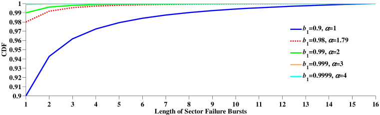
(a) Cumulative distribution functions (CDFs) of the length of sector failure bursts for different $({b}_{1},\alpha)$ values

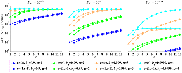
(b) $MTTDL_{sys}$ results of STAIR codes with $\mathbf{e}=(s)$ and $\mathbf{e}=(1,s-1)$ for different $s$’s under different $({b}_{1},\alpha)$ values

Figure 19: $MTTDL_{sys}$ results of STAIR codes with $\mathbf{e}=(s)$ and $\mathbf{e}=(1,s-1)$ for different $s$’s in the correlated sector failure model with different $({b}_{1},\alpha)$ values when $n=8$, $r=16$, and $m=1$.

Figure 19 next shows the impact of the length distribution of sector failure bursts on $MTTDL_{sys}$. Here, we only consider STAIR codes, which can protect against sector failure bursts of any length. Figure 19(a) depicts the burst length distribution for different pairs of $({b}_{1},\alpha)$ that we consider. Smaller values of $b_{1}$ and $\alpha$ imply that the length of a sector failure burst is more likely to be greater than one, or in other words, sector failures are more bursty. Figure 19(b) presents the $MTTDL_{sys}$ results of STAIR codes with $\mathbf{e}=(s)$ and $\mathbf{e}=(1,s-1)$ for different values of $s$ under different pairs of $({b}_{1},\alpha)$. We observe that for more bursty sector failures (e.g., ${b}_{1}=0.9$ and $\alpha=1$), the STAIR code with $\mathbf{e}=(s)$ (for $s\geq 2$) achieves significantly higher reliability than the STAIR code with $\mathbf{e}=(1,s-1)$. In particular, as $s$ increases, the reliability of the STAIR code with $\mathbf{e}=(s)$ increases exponentially. This demonstrates the significance of STAIR codes that support a wider range of $s$. On the other hand, for less bursty sector failures (e.g., ${b}_{1}=0.9999$ and $\alpha=4$), as $s$ increases, the reliability of the STAIR code with $\mathbf{e}=(s)$ increases much more slowly, and in some cases, is even lower than that with $\mathbf{e}=(1,s-1)$ (e.g., when $P_{bit}=10^{-10}$). This observation is consistent with that in the independent sector failure model, in which sector failures are likely scattered across different chunks within a stripe.

8 Related Work

Erasure codes have been widely adopted to provide fault tolerance against device failures in storage systems [37]. Classical erasure codes include standard Reed-Solomon codes [39] and Cauchy Reed-Solomon codes [8], both of which are MDS codes that provide general constructions for all possible configuration parameters. They are usually implemented as systematic codes for storage applications [31, 35, 38], and thus can be used to implement the construction of STAIR codes. In addition, Cauchy Reed-Solomon codes can be further transformed into array codes, whose encoding computations purely build on efficient XOR operations [38].

In the past decades, many kinds of array codes have been proposed, including MDS array codes (e.g., [3, 4, 10, 2, 23, 14, 15, 47, 46, 27, 34]) and non-MDS array codes (e.g., [19, 20, 28]). Array codes are often designed for specific configuration parameters. To avoid compromising the generality of STAIR codes, we do not suggest to adopt array codes in the construction of STAIR codes. Moreover, recent work [36] has shown that Galois Field arithmetic can be implemented to be extremely fast (sometimes at cache line speeds) using SIMD instructions in modern processors.

Sector failures are not explicitly considered in traditional erasure codes, which focus on tolerating device-level failures. To cope with sector failures, ad hoc schemes are often considered. One scheme is scrubbing [43, 29, 41], which proactively scans all disks and recovers any spotted sector failure using the underlying erasure codes. Another scheme is intra-device redundancy [11, 12, 41], in which contiguous sectors in each device are grouped together to form a segment and are then encoded with redundancy within the device. Our work targets a different objective and focuses on constructing an erasure code that explicitly addresses sector failures.

To simultaneously tolerate device and sector failures with minimal redundancy, SD codes [33, 32] (including the earlier PMDS codes [5], which are a subset of SD codes) have recently been proposed. As stated in §1, SD codes are known only for limited configurations and some of the known constructions rely on extensive searches. A relaxation of the SD property has also been recently addressed as a future work [32], which assumes that each row has no more than a given number of sector failures. It is important to note that the relaxation of [32] is different from ours, in which we limit the maximum number of devices with sector failures and the maximum number of sector failures that simultaneously occur in each such device. It turns out that our relaxation enables us to derive a general code construction.

There are other similar kinds of erasure codes that have similar constructions to STAIR codes but serve for different purposes. Blaum et al. [6] have constructed a family of nested codes that define the number of tolerable sector failures in each row for an SSD array in which sector failures appear as worn-out blocks. However, unlike STAIR codes, such nested codes do not consider sector failure bursts [1, 41]. Another kind of erasure codes is the family of locally repairable codes (LRCs) [22, 21, 40], which focus on improving the recovery performance of storage systems. Pyramid codes [21] are designed for small-scale device failures and have been implemented in archival storage [45]. Huang et al.’s and Sathiamoorthy et al.’s LRCs [22, 40] can be viewed as generalizations of Pyramid codes and are recently adopted in commercial storage systems. In particular, Huang et al.’s LRCs [22] achieve the same fault tolerance property as PMDS codes [5], and thus can also be used as SD codes. However, the construction of Huang et al.’s LRCs is limited to $m=1$ only. To the best of our knowledge, STAIR codes are the first general family of erasure codes that can efficiently tolerate both device and sector failures.

9 Conclusions

We present STAIR codes, a general family of erasure codes that can tolerate simultaneous device and sector failures in a space-efficient manner. STAIR codes can be constructed for tolerating any numbers of device and sector failures subject to a pre-specified sector failure coverage. The special construction of STAIR codes also makes efficient encoding/decoding possible through parity reuse. Compared to the recently proposed SD codes [5, 33, 32], STAIR codes not only support a much wider range of configuration parameters, but also achieve higher encoding/decoding speed based on our experiments.

The source code of STAIR codes is available at http://ansrlab.cse.cuhk.edu.hk/software/stair.

APPENDIX

Appendix A Proof of Homomorphic Property

We formally prove the homomorphic property described in §4.1. We state the following theorem.

Theorem A.1

In the construction of the canonical stripe of STAIR codes, the encoding of each chunk in the column direction via $\mathcal{C}_{col}$ is homomorphic, such that each augmented row in the canonical stripe is a codeword of $\mathcal{C}_{row}$.

Proof: We prove by matrix operations. We define the matrices $\mathbf{D}=[d_{i,j}]_{r\times(n-m)}$, $\mathbf{P}=[p_{i,k}]_{r\times m}$, and $\mathbf{P}^{\prime}=[p^{\prime}_{i,l}]_{r\times m^{\prime}}$. Also, we define the generator matrices $\mathbf{G}_{row}$ and $\mathbf{G}_{col}$ for the codes $\mathcal{C}_{row}$ and $\mathcal{C}_{col}$, respectively, as:

$$\mathbf{G}_{row} = \left(\mathbf{I}_{(n-m)\times(n-m)}\mid\mathbf{A}_{(n-m)\times(m+m^{\prime})}\right),$$

$$\mathbf{G}_{col} = \left(\mathbf{I}_{r\times r}\mid\mathbf{B}_{r\times e_{m^{\prime}-1}}\right),$$

where $\mathbf{I}$ is an identity matrix, and $\mathbf{A}$ and $\mathbf{B}$ are the sub-matrices that form the parity symbols. The upper $r$ rows of the stripe can be expressed as follows:

$$\left(\mathbf{D}\mid\mathbf{P}\mid\mathbf{P}^{\prime}\right) = \mathbf{D}\cdot\mathbf{G}_{row}.$$

The lower $e_{m^{\prime}-1}$ augmented rows are expressed as follows:

$$\left(\left(\mathbf{D}\mid\mathbf{P}\mid\mathbf{P}^{\prime}\right)^{T}\cdot\mathbf{B}\right)^{T} = \mathbf{B}^{T}\cdot\left(\mathbf{D}\cdot\mathbf{G}_{row}\right)$$

$$= \left(\mathbf{B}^{T}\cdot\mathbf{D}\right)\cdot\mathbf{G}_{row}$$

We can see that each of the lower $e_{m^{\prime}-1}$ rows can be calculated using the generator matrix $\mathbf{G}_{row}$, and hence is a codeword of $\mathcal{C}_{row}$. $\hfill\Box$

Appendix B Explicit Expressions of $P_{str}$ for Various Erasure Codes

B.1 Reed-Solomon Codes

The explicit expression of $P_{str}$ for Reed-Solomon codes is as follows:

$$P_{str}=1-P_{chk(0)}^{n-m}.$$ (18)

B.2 STAIR Codes

Explicit expressions of $P_{str}$ for some STAIR codes with special $\mathbf{e}$’s are as follows:

1. For a STAIR code with $\mathbf{e}=(s)$ for $s\geq 1$,

   $$P_{str}=1-P_{chk(0)}^{n-m}-{n-m\choose 1}\cdot\sum\limits_{i=1}^{s}P_{chk(i)}\cdot P_{chk(0)}^{n-m-1}.$$ (19)

2. For a STAIR code with $\mathbf{e}=(1,s-1)$ for $s\geq 2$,

   $$\begin{split}P_{str}=&1-P_{chk(0)}^{n-m}-{n-m\choose 1}\cdot\sum\limits_{i=1}^{s-1}P_{chk(i)}\cdot P_{chk(0)}^{n-m-1}-\\ &{n-m\choose 2}\cdot P_{chk(1)}^{2}\cdot P_{chk(0)}^{n-m-2}-{n-m\choose 1}\cdot{n-m-1\choose 1}\cdot\sum\limits_{i=2}^{s-1}P_{chk(i)}\cdot P_{chk(1)}\cdot P_{chk(0)}^{n-m-2}.\end{split}$$ (20)

3. For a STAIR code with $\mathbf{e}=(2,s-2)$ for $s\geq 4$,

   $$\begin{split}P_{str}=&1-P_{chk(0)}^{n-m}-{n-m\choose 1}\cdot\sum\limits_{i=1}^{s-2}P_{chk(i)}\cdot P_{chk(0)}^{n-m-1}-\\ &{n-m\choose 2}\cdot P_{chk(1)}^{2}\cdot P_{chk(0)}^{n-m-2}-{n-m\choose 1}\cdot{n-m-1\choose 1}\cdot\sum\limits_{i=2}^{s-2}P_{chk(i)}\cdot P_{chk(1)}\cdot P_{chk(0)}^{n-m-2}-\\ &{n-m\choose 2}\cdot P_{chk(2)}^{2}\cdot P_{chk(0)}^{n-m-2}-{n-m\choose 1}\cdot{n-m-1\choose 1}\cdot\sum\limits_{i=3}^{s-2}P_{chk(i)}\cdot P_{chk(2)}\cdot P_{chk(0)}^{n-m-2}.\end{split}$$ (21)

4. For a STAIR code with $\mathbf{e}=(1,1,s-2)$ for $s\geq 3$,

   $$\begin{split}P_{str}=&1-P_{chk(0)}^{n-m}-{n-m\choose 1}\cdot\sum\limits_{i=1}^{s-2}P_{chk(i)}\cdot P_{chk(0)}^{n-m-1}-\\ &{n-m\choose 2}\cdot P_{chk(1)}^{2}\cdot P_{chk(0)}^{n-m-2}-{n-m\choose 1}\cdot{n-m-1\choose 1}\cdot\sum\limits_{i=2}^{s-2}P_{chk(i)}\cdot P_{chk(1)}\cdot P_{chk(0)}^{n-m-2}-\\ &{n-m\choose 3}\cdot P_{chk(1)}^{3}\cdot P_{chk(0)}^{n-m-3}-{n-m\choose 2}\cdot{n-m-2\choose 1}\cdot\sum\limits_{i=2}^{s-2}P_{chk(i)}\cdot P_{chk(1)}^{2}\cdot P_{chk(0)}^{n-m-3}.\\ \end{split}$$ (22)

5. For a STAIR code with $\mathbf{e}=(\overset{s}{\overbrace{1,1,\cdots,1}})$ for $s\geq 1$,

   $$P_{str}=1-\sum\limits_{i=0}^{s}\left({n-m\choose i}\cdot P_{chk(1)}^{i}\cdot P_{chk(0)}^{n-m-i}\right).$$ (23)

B.3 SD Codes

Explicit expressions of $P_{str}$ for SD codes with $s\leq 3$ [33, 32] are as follows:

1. For an SD code with $s=1$,

   $$P_{str}=1-P_{chk(0)}^{n-m}-{n-m\choose 1}\cdot P_{chk(1)}\cdot P_{chk(0)}^{n-m-1}.$$ (24)

2. For an SD code with $s=2$,

   $$P_{str}=1-P_{chk(0)}^{n-m}-{n-m\choose 1}\cdot\sum\limits_{i=1}^{2}P_{chk(i)}\cdot P_{chk(0)}^{n-m-1}-{n-m\choose 2}\cdot P_{chk(1)}^{2}\cdot P_{chk(0)}^{n-m-2}.$$ (25)

3. For an SD code with $s=3$,

   $$\begin{split}P_{str}=&1-P_{chk(0)}^{n-m}-{n-m\choose 1}\cdot\sum\limits_{i=1}^{3}P_{chk(i)}\cdot P_{chk(0)}^{n-m-1}-\\ &{n-m\choose 2}\cdot P_{chk(1)}^{2}\cdot P_{chk(0)}^{n-m-2}-{n-m\choose 1}\cdot{n-m-1\choose 1}\cdot P_{chk(2)}\cdot P_{chk(1)}\cdot P_{chk(0)}^{n-m-2}-\\ &{n-m\choose 3}\cdot P_{chk(1)}^{3}\cdot P_{chk(0)}^{n-m-3}.\end{split}$$ (26)

References

- [1] L. N. Bairavasundaram, G. R. Goodson, S. Pasupathy, and J. Schindler. An analysis of latent sector errors in disk drives. In Proceedings of the 2007 ACM SIGMETRICS International Conference on Measurement and Modeling of Computer Systems (SIGMETRICS ’07), pages 289–300, San Diego, CA, June 2007.
- [2] M. Blaum. A family of MDS array codes with minimal number of encoding operations. In Proceedings of the 2006 IEEE International Symposium on Information Theory (ISIT ’06), pages 2784–2788, Seattle, WA, July 2006.
- [3] M. Blaum, J. Brady, J. Bruck, and J. Menon. EVENODD: An efficient scheme for tolerating double disk failures in RAID architectures. IEEE Transactions on Computers, 44(2):192–202, 1995.
- [4] M. Blaum, J. Bruck, and A. Vardy. MDS array codes with independent parity symbols. IEEE Transactions on Information Theory, 42(2):529–542, 1996.
- [5] M. Blaum, J. L. Hafner, and S. Hetzler. Partial-MDS codes and their application to RAID type of architectures. IEEE Transactions on Information Theory, 59(7):4510–4519, July 2013.
- [6] M. Blaum, J. L. Hafner, and S. R. Hetzler. Nested multiple erasure correcting codes for storage arrays. U.S. Patent Application No. 13/036,845, Aug. 2012.
- [7] M. Blaum and J. S. Plank. Construction of sector-disk (SD) codes with two global parity symbols. IBM Research Report RJ10511 (ALM1308-007), Almaden Research Center, IBM Research Division, Aug. 2013.
- [8] J. Blomer, M. Kalfane, R. Karp, M. Karpinski, M. Luby, and D. Zuckerman. An XOR-based erasure-resilient coding scheme. Technical Report TR-95-048, International Computer Science Institute, UC Berkeley, Aug. 1995.
- [9] S. Boboila and P. Desnoyers. Write endurance in flash drives: Measurements and analysis. In Proceedings of the 8th USENIX Conference on File and Storage Technologies (FAST ’10), pages 115–128, San Jose, CA, Feb. 2010.
- [10] P. Corbett, B. English, A. Goel, T. Grcanac, S. Kleiman, J. Leong, and S. Sankar. Row-diagonal parity for double disk failure correction. In Proceedings of the 3rd USENIX Conference on File and Storage Technologies (FAST ’04), pages 1–14, San Francisco, CA, Mar. 2004.
- [11] A. Dholakia, E. Eleftheriou, X.-Y. Hu, I. Iliadis, J. Menon, and K. Rao. A new intra-disk redundancy scheme for high-reliability RAID storage systems in the presence of unrecoverable errors. ACM Transactions on Storage, 4(1):1–42, 2008.
- [12] A. Dholakia, E. Eleftheriou, X.-Y. Hu, I. Iliadis, J. Menon, and K. Rao. Disk scrubbing versus intradisk redundancy for RAID storage systems. ACM Transactions on Storage, 7(2):1–42, 2011.
- [13] P. Elias. Error-free coding. IRE Transactions on Information Theory, 4(4):29–37, Sept. 1954.
- [14] G. Feng, R. Deng, F. Bao, and J. Shen. New efficient MDS array codes for RAID Part I: Reed-Solomon-like codes for tolerating three disk failures. IEEE Transactions on Computers, 54(9):1071–1080, 2005.
- [15] G. Feng, R. Deng, F. Bao, and J. Shen. New efficient MDS array codes for RAID Part II: Rabin-like codes for tolerating multiple () disk failures. IEEE Transactions on Computers, 54(12):1473–1483, 2005.
- [16] K. M. Greenan, J. S. Plank, and J. J. Wylie. Mean time to meaningless: MTTDL, Markov models, and storage system reliability. In Proceedings of the 2nd Workshop on Hot Topics in Storage and File Systems (HotStorage ’10), pages 1–5, Boston, MA, June 2010.
- [17] L. M. Grupp, A. M. Caulfield, J. Coburn, S. Swanson, E. Yaakobi, P. H. Siegel, and J. K. Wolf. Characterizing flash memory: Anomalies, observations, and applications. In Proceedings of the 42nd International Symposium on Microarchitecture (MICRO ’09), pages 24–33, New York, NY, Dec. 2009.
- [18] L. M. Grupp, J. D. Davis, and S. Swanson. The bleak future of NAND flash memory. In Proceedings of the 10th USENIX conference on File and Storage Technologies (FAST ’12), pages 17–24, San Jose, CA, Feb. 2012.
- [19] J. L. Hafner. WEAVER codes: Highly fault tolerant erasure codes for storage systems. In Proceedings of the 4th USENIX Conference on File and Storage Technologies (FAST ’05), pages 211–224, San Francisco, CA, Dec. 2005.
- [20] J. L. Hafner. HoVer erasure codes for disk arrays. In Proceedings of the 2006 International Conference on Dependable Systems and Networks (DSN ’06), pages 1–10, Philadelphia, PA, June 2006.
- [21] C. Huang, M. Chen, and J. Li. Pyramid codes: Flexible schemes to trade space for access efficiency in reliable data storage systems. ACM Transactions on Storage, 9(1):1–28, Mar. 2013.
- [22] C. Huang, H. Simitci, Y. Xu, A. Ogus, B. Calder, P. Gopalan, J. Li, and S. Yekhanin. Erasure coding in Windows Azure storage. In Proceedings of the 2012 USENIX Annual Technical Conference (USENIX ATC ’12), pages 15–26, Boston, MA, June 2012.
- [23] C. Huang and L. Xu. STAR: An efficient coding scheme for correcting triple storage node failures. In Proceedings of the 4th USENIX Conference on File and Storage Technologies (FAST ’05), pages 889–901, San Francisco, CA, Dec. 2005.
- [24] I. Iliadis and X.-Y. Hu. Reliability assurance of RAID storage systems for a wide range of latent sector errors. In Proceedings of the 2008 IEEE International Conference on Networking, Architecture, and Storage (NAS ’08), pages 10–19, Chongqing, China, June 2008.
- [25] Intel Corporation. Intelligent RAID 6 theory — overview and implementation. White Paper, 2005.
- [26] M. Li and P. P. C. Lee. STAIR codes: A general family of erasure codes for tolerating device and sector failures in practical storage systems. In Proceedings of the 12th USENIX Conference on File and Storage Technologies (FAST ’14), pages 147–162, Santa Clara, CA, Feb. 2014.
- [27] M. Li and J. Shu. C-Codes: Cyclic lowest-density MDS array codes constructed using starters for RAID 6. IBM Research Report RC25218 (C1110-004), China Research Laboratory, IBM Research Division, Oct. 2011.
- [28] M. Li, J. Shu, and W. Zheng. GRID codes: Strip-based erasure codes with high fault tolerance for storage systems. ACM Transactions on Storage, 4(4):1–22, 2009.
- [29] A. Oprea and A. Juels. A clean-slate look at disk scrubbing. In Proceedings of the 8th USENIX Conference on File and Storage Technologies (FAST ’10), pages 1–14, San Jose, CA, Feb. 2010.
- [30] E. Pinheiro, W.-D. Weber, and L. A. Barroso. Failure trends in a large disk drive population. In Proceedings of the 5th USENIX conference on File and Storage Technologies (FAST ’07), pages 17–28, San Jose, CA, Feb. 2007.
- [31] J. S. Plank. A tutorial on Reed-Solomon coding for fault-tolerance in RAID-like systems. Software — Practice & Experience, 27(9):995–1012, 1997.
- [32] J. S. Plank and M. Blaum. Sector-disk (SD) erasure codes for mixed failure modes in RAID systems. ACM Transactions on Storage, 10(1):1–17, Jan. 2014.
- [33] J. S. Plank, M. Blaum, and J. L. Hafner. SD codes: Erasure codes designed for how storage systems really fail. In Proceedings of the 11th USENIX conference on File and Storage Technologies (FAST ’13), pages 95–104, San Jose, CA, Feb. 2013.
- [34] J. S. Plank, A. L. Buchsbaum, and B. T. Vander Zanden. Minimum density RAID-6 codes. ACM Transactions on Storage, 6(4):1–22, May 2011.
- [35] J. S. Plank and Y. Ding. Note: Correction to the 1997 tutorial on Reed-Solomon coding. Software — Practice & Experience, 35(2):189–194, 2005.
- [36] J. S. Plank, K. M. Greenan, and E. L. Miller. Screaming fast Galois Field arithmetic using Intel SIMD instructions. In Proceedings of the 11th USENIX conference on File and Storage Technologies (FAST ’13), pages 299–306, San Jose, CA, Feb. 2013.
- [37] J. S. Plank and C. Huang. Tutorial: Erasure coding for storage applications. Slides presented at FAST-2013: 11th Usenix Conference on File and Storage Technologies, Feb. 2013.
- [38] J. S. Plank and L. Xu. Optimizing Cauchy Reed-Solomon codes for fault-tolerant network storage applications. In Proceedings of the 5th IEEE International Symposium on Network Computing and Applications (NCA ’06), pages 173–180, Cambridge, MA, July 2006.
- [39] I. S. Reed and G. Solomon. Polynomial codes over certain finite fields. Journal of the Society for Industrial and Applied Mathematics, 8(2):300–304, 1960.
- [40] M. Sathiamoorthy, M. Asteris, D. Papailiopoulous, A. G. Dimakis, R. Vadali, S. Chen, and D. Borthakur. XORing elephants: Novel erasure codes for big data. In Proceedings of the 39th International Conference on Very Large Data Bases (VLDB ’13), pages 325–336, Trento, Italy, Aug. 2013.
- [41] B. Schroeder, S. Damouras, and P. Gill. Understanding latent sector errors and how to protect against them. In Proceedings of the 8th USENIX Conference on File and Storage Technologies (FAST ’10), pages 71–84, San Jose, CA, Feb. 2010.
- [42] B. Schroeder and G. A. Gibson. Disk failures in the real world: What does an MTTF of 1,000,000 hours mean to you? In Proceedings of the 5th USENIX conference on File and Storage Technologies (FAST ’07), pages 1–16, San Jose, CA, Feb. 2007.
- [43] T. J. E. Schwarz, Q. Xin, E. L. Miller, and D. D. E. Long. Disk scrubbing in large archival storage systems. In Proceedings of the 12th Annual Meeting of the IEEE/ACM International Symposium on Modeling, Analysis, and Simulation of Computer and Telecommunication Systems (MASCOTS ’04), pages 409–418, Volendam, Netherlands, Oct. 2004.
- [44] J. White and C. Lueth. RAID-DP: NetApp implementation of double-parity RAID for data protection. Technical Report TR-3298, NetApp, Inc., May 2010.
- [45] A. Wildani, T. J. E. Schwarz, E. L. Miller, and D. D. Long. Protecting against rare event failures in archival systems. In Proceedings of the 17th Annual Meeting of the IEEE/ACM International Symposium on Modelling, Analysis and Simulation of Computer and Telecommunication Systems (MASCOTS ’09), pages 1–11, London, UK, Sept. 2009.
- [46] L. Xu, V. Bohossian, J. Bruck, and D. G. Wagner. Low-density MDS codes and factors of complete graphs. IEEE Transactions on Information Theory, 45(6):1817–1826, Sept. 1999.
- [47] L. Xu and J. Bruck. X-Code: MDS array codes with optimal encoding. IEEE Transactions on Information Theory, 45(1):272–276, 1999.
- [48] M. Zheng, J. Tucek, F. Qin, and M. Lillibridge. Understanding the robustness of SSDs under power fault. In Proceedings of the 11th USENIX conference on File and Storage Technologies (FAST ’13), pages 271–284, San Jose, CA, Feb. 2013.