On possible origins of trends
in financial market price changes

Abstract

We investigate possible origins of the trend in financial markets, where trend we refer to as is a relatively long-term fluctuation observed in price change (price movement), using a simple deterministic threshold model that contains no external driving force term to generate trends forcibly. We find that the trend can be generated by this simple model without any external driving force. Furthermore, from thorough numerical simulations, we obtain two following results: (i) a trend of monotonic increase or decrease can be generated only by dealers’ minuscule price updates for the next deal trying to follow an expected forthcoming direction of price change, (ii) non-monotonic trends spontaneously emerge when dealers cannot obtain accurate information about the number of dealers participating in the next deal. We conclude from these results that the emergence of trends is not necessarily generated by an external driving force but an natural outcome of the accumulation of minuscule price updates of individual dealers with insufficient information about the next deal.

1 Introduction

Many phenomena in human society are dominated by human choices. Buying and selling is one of them, and we regard financial markets as an aggregation of dealers’ choices and their interactions. A major indicator in a financial market is its price change (price movement). Generally speaking, price change in financial markets fluctuates irregularly, as shown in Fig. 1. However, the mechanism of the fluctuations has not been elucidated yet, and the question still remains to be challenging. There are two major approaches to tackle the question. One is to investigate features or natures of the data generated by a dynamical system from the viewpoint of statistics [1, 2, 3], and the other is to construct an artificial market using a model and investigate events in the market [4, 5, 6, 7, 8, 9, 10, 11]. The merit of the former approach is that it provides us with various knowledge and insights for the understandings of the nature of price changes. However, this approach is restrictive, because it does not always lead us to a deeper understanding of the mechanism of price changes produced by the interaction between dealers’ choices and various market price properties [10]. In contrast, the latter approach significantly contributes to clarifying the mechanism. As the purpose of this paper is to find possible origins of relatively long-term fluctuations generally observed in financial market price changes, which we refer to as “trends,” we follow the latter approach (we will describe the details of our definition of trends later).

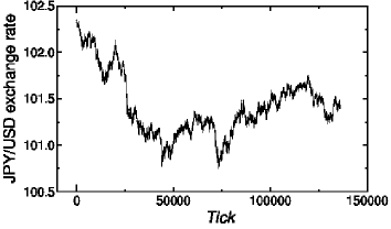
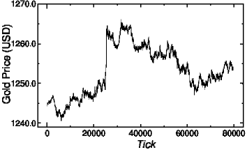
Figure 1: Examples of price changes in financial markets showing short-term variabilities and trends: (a) Tick data of Japanese Yen/US dollar (JPY/USD) exchange rate and (b) tick data of gold price at New York Mercantile Exchange (NYMEX) futures. Both the data are taken for 48 hours from twelve midnight on 3 February 2014 to twelve midnight on 4 February 2014. The data can be obtained from http://ratedata.gaincapital.com/

Some models, which are categorized as the dealer model, have been proposed [4, 5, 11]. The dealer model is an agent-based model and constructs an artificial market. The first dealer model was introduced by Takayasu et al. in 1992 [4]. They considered that a market is composed of many dealers and buying and selling are interactions among them with discontinuous (nonlinear) and irreversible processes. To implement this mechanism they introduced a numerical model of financial market prices using threshold dynamics [4]. In the model a deterministic dynamics is assumed for an assembly of agents describing mutual trades by threshold dynamics including discontinuous irreversible interactions. After this pioneering work, numerous studies have been done (for example, see Refs. [5, 6, 7, 8, 9, 10, 11]), aiming for improvement and refinement to be able to reproduce basic empirical laws such as the power-law distribution of price changes, slow decay of auto-correlation of volatility, and so on. For the details see [11].

In this paper, we observe afresh the behaviours of financial market data carefully. As mentioned above, price changes in financial markets show irregular fluctuations (see Fig. 1). These irregular fluctuations are usually divided into two main features, short-term variabilities and “trends.” However, we would like to emphasize that this separation seems to be done rather arbitrary by simple visual inspection. A trend we recognize is a general or rough direction of continuous movement such as upward, downward or sideways during an arbitrary “long” period of observation compared to the unit time length for taking time series data of price change. If we take a longer observational time, a trend in a certain period might be considered as a mere fluctuation around another large trend in the longer period of time (See Fig. 2). Whether a movement in price change is recognized as a short-term fluctuation or a trend is, therefore, a matter of observational time scale and the separation is rather arbitrary. This is our definition for trends and we recognize trends by this definition.

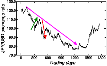
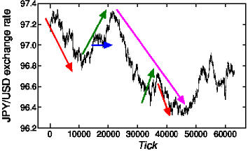
Figure 2: (Colour online) Examples of “trends” we recognize: (a) daily JPY/USD exchange rate from 2 January 2007 to 31 December 2013 and (b) tick data of JPY/USD exchange rate for 24 hours in 7 August 2013 (Wednesday). Although the data are in different resolutions, we can recognize some trends that are marked by the arrows. We note that a longer downward trend includes shorter upward and downward trends in (a) and (b).

It should also be noted that there seems to be a vague consensus that trends are driven by some external factors such as economical fundamentals and that short-term variabilities are fluctuations around these trends due to stochastic nature of individual deals. Hence, existing models seems to have been built or improved based on this consensus dealing with these two fluctuations (short-term variabilities and trends) separately. A possible origin for the short-term variabilities has already been indicated by Takayasu et al. [4]. Despite of numerous works after the work, curious to say, discussions on the origins of trends does not seem to be lively, although market participants are used to pay more attention to the trend rather than the details of the short-term variabilities to gain information of the overall movement of markets.

One of the major underlying reasons seems to be that the existence of the trends is taken to be granted as those driven by some external factors, such as economical fundamentals (for example, the gross domestic product (GDP) varying according to policy interest rate, remarks by senior administration officials or central bankers, and so on) and technical analyses of economists. On the other hand, it is well known that the trends can also be observed without any remarkable news about important economic index changes to be released. Hence, it brings up a following simple question on the origin of trends: if it were not for these external factors, do trends completely disappear? We focus our attention mainly on this point.

The key idea for the present work is the following. Generally speaking, to understand a certain phenomenon we need the information about its structure, mechanism, situation, condition and so on. However, it is usually impossible to obtain the entire information. Although this fact seems to be trivial, we will show that trends can emerge indeed only from this simple and trivial basis. The conclusion indicates that there is no clear time scale for dividing the price change clearly into short-term variabilities and trends. Both of them spontaneously emerge at the same time. In this regard, a trend is not a dynamical movement generated by some external driving force but is an accumulation of microscopic price updates of individual dealers due to flimsy expectations. In this paper, we show two results obtained by our investigation based on this idea. First, we show that a trend of monotonic increase or decrease can be generated within the framework of the simplest dealer model with no external driving force only by including the effect of dealers’ minuscule price updates for the next deal trying to follow an expected forthcoming direction of the price change. Next, we show that non-monotonic trends spontaneously emerge when dealers cannot obtain accurate information about the number of dealers participating in the next deal. This result implies that trends are spontaneously generated even if the influence of fundamentals and technical analyses on financial markets is very weak or even absent and suggests a possible unknown mechanism for generation of trends.

It should be mentioned here that, although we understand that it is important to reproduce basic empirical characteristics of real data, we do not aspire for the reproduction in this paper. We simply focus on possible origins of trends.

This paper is organized as follows. We start from an existing deterministic dealer model with threshold elements and add some essential modifications to the original dealer model based on the key idea of dealers’ incomplete information acquisition of the next deal. In Section 2, we briefly review the original dealer model and its basic behaviours. In Section 3 we extend the original dealer model to include microscopic and distinctive price updates of individual dealers and show that trends are generated only by this extension without introducing any external driving force term. Section 4 is for the discussions and summary.

2 Current technologies: deterministic threshold dealer model

To generate trends and find possible (or unknown) origins of trends, we use a previously proposed deterministic dealer model with threshold elements. As the original model is proposed in 1992 by Takayasu et al. [4], we refer to the model as the “dealer model 92.” Since the dealer model 92 is deterministic including no probabilistic factor, we expect that we are able to have a better sense of the behaviours generated by the model. As the model treats price change of all deals, the price data generated by the model should be compared to tick data. For simplicity the deals in the model are assumed to be concerning to only one brand in one market. Also, we assume that all dealers participate deals with the same rule.

After the dealer model 92 was proposed, some modifications have been made [5, 10, 11]. However, we consider that the modifications are artificial, since all deals are done by only two dealers, that is, one buyer and one seller. In the actual deals there are usually more than one sellers, which we consider is one of the vital aspects of deals. As the dealer model 92 treats such a situation, we adopt the dealer model 92.

In this section we briefly review the dealer model 92 and clarify the mechanism of the price change.

2.1 Dealer model 92

Deals, composed of consecutive selling and buying, form a typical discontinuous and irreversible process. A deal is done, if a buying condition and a selling condition meet, while it is undone, if not. This is the origin of the discontinuity. The buyer and the seller of the last deal would never deal again under the identical condition at least for a while. This is the origin of the irreversibility. The dealer model 92 is introduced to reflect these aspects of dealing and we here begin by following the basic settings of the original model [4].

The market is composed of $N$ dealers. Let the $i$-th dealer’s buying price and selling price be $B_{i}$ and $S_{i}$, respectively. The selling price $S_{i}$ is larger than the buying price $B_{i}$, and the difference $L_{i}=S_{i}-B_{i}$ is always positive. For simplicity we use a constant value $L$ for all $L_{i}$ [4]. This simplification gives $L=S_{i}-B_{i}$ for all $i$. A deal is done between pairs of $i$ and $j$ when $B_{i}\geq S_{j}$. In this model, a deal among all dealers is done when the following condition is satisfied:

$$\max\{B_{i}\}-\min\{B_{i}\}\geq L,$$ (1)

where $\max\{B_{i}\}$ and $\min\{B_{i}\}$ indicate the maximum and minimum values. In the dealer model 92 there is one buyer and one or more than one sellers. The buyer $i$ is the dealer who gives the highest buying price $B_{i}$ and can buy at the price $B_{i}$ from other dealers $j$ who satisfy the following selling condition

$$\max\{B_{i}\}-\{B_{j}\}\geq L.$$

The price $P(t)$ of the deal is therefore defined by the $\max\{B_{i}\}$. If Eq. (1) is not satisfied, the deal is not done and the market price does not change. Hence,

$$P(t)=\begin{cases}\max\{B_{i}\}&\text{(when a deal is done)},\\ P(t-1)&\text{(when a deal is not done)}.\end{cases}$$ (2)

When a deal is done, there are one buyer, sellers who could make the deal, and the remainders who could not participate in the deal. However, the remainder do not look wistfully and enviously at the deal with doing nothing. As all dealers are potentially willing to participate in the deals, they re-establish their prices for the next deal. Obviously, dealers who want to buy need to offer higher price and dealers who want to sell need to offer cheaper price. To reflect the eagerness to participate in the next deal, the $i$-th dealer’s expectation $a_{i}$ is introduced. The term represent a character of the $i$-th dealer. If $a_{i}>0$, the dealer raises the price setting, and if $a_{i}<0$, the dealer lowers the price setting. That is, dealers with $a_{i}>0$ and $a_{i}<0$ take the actions as buyers and sellers, respectively.

In this model each dealer is assumed to have his/her own expectation. Hence, the values of $a_{i}$ are chosen from uniform random numbers in a range and the mean of $\{a_{i}\}$ is set to be zero, which keeps the overall expectations of dealers for buying and selling in equilibrium. As dealers becomes buyers and sellers depending on their conditions and circumstances in the actual financial markets, the details inside of the deals are very complicated. To simplify the situation, however, as the model assumes that all dealers have infinitely large amount of property, the dealers do not change their attitudes even if a deal is done (that is, the sign of $a_{i}$ does not change) [4, 5]. Also, this model is assumed to be in an invariant state (steady state). Hence, the values of $a_{i}$ do not change once assigned [4].

An unique aspect of this model is that it takes into account an acquisitive nature of the buyer and sellers for the next deal. It is assumed that the buyer and sellers who could participate a deal expect that they can participate again in the next deal with a cheaper price for the buyer and a higher price for the sellers. The other dealers who could not participate in the previous deal do not have such a psychological tendency. To reflect such a tendency, the term $\Delta_{i}$ is introduced:

$$\Delta_{i}=\begin{cases}-\delta&\text{(for the buyer)},\\ \delta/n&\text{(for the sellers)},\\ 0&\text{(for the nonparticipants of the deal)},\end{cases}$$ (3)

where $0<\delta<L$ and $n$ is the number of the sellers of the deal. That is, the next buying price of the buyer falls by the amount of $\delta$ from the current buying price and the next selling prices of the sellers rises by the amount of $\delta/n$ from the current selling prices. The buyer and sellers who could not participate in the next deal have no anticipation. Also, when Eq. (1) is not satisfied (that is, a deal is not done), $\Delta_{i}=0$ for all $i$. Note that the summation of all $\Delta_{i}$ is zero.

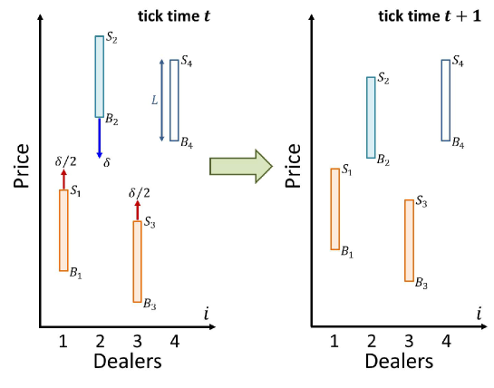
Figure 3: (Colour online) Schematic diagram of $\Delta$ from time $t$ to $t+1$ when Eq. (1) is satisfied. The length of each vertical bar is the constant $L$. The top and bottom of each bar correspond to the upper and lower threshold price of each dealer, respectively. The $\Delta$ of the buyer is $-\delta$ and that of the sellers is $\delta/n$, where $0<\delta<L$ and $n$ is the number of the sellers. The value of $\delta$ is constant defined by Eq. (3). In this figure the buyer is $i=2$, the sellers are $i=1$ and $3$ ($n=2$), and the dealer $i=4$ does not participate in the deal.

Based on these ideas, the price update for the $i$-th dealer in the dealer model 92 is given by

$$B_{i}(t+1)=B_{i}(t)+\Delta_{i}(t)+a_{i}+c_{i}\{P(t)-P(t_{\text{prev}})\},$$ (4)

where the term $c_{i}$ characterizes the $i$-th dealer’s response to the change of market price and $t_{\text{prev}}$ indicates the time when the last deal is done [4]. The behaviour of Eq. (4) has already been scrutinized for various values of $c_{i}$, $a_{i}$ and the number of dealers, $n$ and it is commonly known that Eq. (4) is extremely unstable and uncontrollable when $c_{i}~{}\neq~{}0$ [4, 12]. For details see [12]. Hence, we use Eq. (4) with $c_{i}=0$ as the dealer model 92 for the starting point of our work, which becomes

$$B_{i}(t+1)=B_{i}(t)+\Delta_{i}(t)+a_{i}.$$ (5)

2.2 Typical behaviours of the dealer model 92

We show typical behaviours generated by the dealer model 92 with Eq. (3) for $\Delta_{i}$. To generate the data we take the number of dealers $N=100$ and $\delta=0.4$. The initial value of $B_{i}(t)$ is taken from uniform random numbers in the range $(-L,L)$ with $L=1$. The values of $a_{i}$ in Eq. (5) are taken from uniform random numbers in the range $(-\alpha,\alpha)$ with $\alpha=0.01$. As mentioned above, to equalize dealers’ eagerness for buying and selling, the mean of $\{a_{i}\}$ in Eq. (5) is set to be zero.

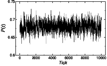
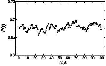
Figure 4: Typical behaviours of simulated price data $P(t)$ of the dealer model 92, Eq. (5), with Eq. (3), where (b) is an enlargement of (a), and both of black circle mark and line are used to show details of price changes in (b). For the model $N=100$, $L=1$, $\alpha=0.01$ and $\delta=0.4$ are used. The value of $a_{i}$ and the initial condition of $B_{i}(t)$ are taken from uniform random numbers in the ranges $(-\alpha,\alpha)$ and $(-L,L)$, respectively.

Figure 4 shows the typical behaviours of price data $P(t)$, where we use the price data only when the deal is done. In Fig. 4(a), it is shown that the behaviours are stable over long periods and $P(t)$ fluctuates around the mean value showing short-term variabilities but does not have trends. Figure 4(b) shows that the price $P(t)$ does not change drastically but slightly over time.

2.3 Some observations and possible reasons for lacking of trends

The zero value of the mean of the dealer’s expectation $\{a_{i}\}$ means that the overall summation of the dealer’s expectation is zero. We note that this does not necessarily mean that the number of dealers with $a_{i}>0$ should be the same as that of dealers with $a_{i}<0$. The number of the dealers with $a_{i}>0$ for Fig. 4 is 38 where the number of the total dealers is 100. From the observations, trends do not appear when dealers’ expectations for buying and selling equal out. In other words, breaking the balance of dealers’ expectation of buying and selling could be vital for generating trends. Based on this idea, we make attempts to generate trends under some well-defined situations in the next section.

3 Exploration of origins for trends

In this section we make attempts to generate trends by extending the dealer model 92 to the directions suitable to two realistic situations. The one is the trend with supposition. We show that a trend emerges from the intention of individual dealers following to the expected direction of forthcoming price change. The other is the trend with no supposition. We show that a trend emerges almost spontaneously only from incomplete information of the dealers even if they do not have any intention for the deals. After considering these two trends separately, we combine both ideas into one model and generate data using it.

3.1 Trends with supposition: premeditated trends

We show here that we are able to generate monotonic increase or decrease trends at our disposal only by introducing the effect of intentions of individual dealers following to the expected direction of forthcoming price change. It is widely believed that continuous trends in relatively long-terms are generated by fundamentals. It is considered that fundamentals influence dealers’ longer-term intention and the major trends in the relative long term are believed to be generated by the dealers’ supposition. We consider that the effect of fundamentals comes into the dealer model through the supposition of dealers for the direction of the price change in a relatively long term due to the changes in fundamentals.

As Eqs. (3) and (5) show, when a deal is done, the buyer brings down the asking price for the next deal, expecting that it might be possible to buy at a cheaper price. Similarly, when a deal is done, the sellers bring up their selling prices for the next deal, expecting that it might be possible to sell at a higher price.

How does the acquisitiveness change in the existence of an expected direction of price change in a market? When an increase (or decrease) direction of price change is expected in a market, it seems to be plausible that a dealer, whether the dealer is either a buyer or a seller, considers that other dealers are also not likely to take the same attitude in the next deal if the dealer offers a higher (or cheaper) price. To incorporate this idea, we redefine Eq. (3) with the small values $\varepsilon_{b}$ and $\varepsilon_{s}$ as follows:

$$\Delta_{i}=\begin{cases}-\delta\times(1.0+\varepsilon_{b})&\text{(for the buyer)},\\ (\delta\times\varepsilon_{s})/n&\text{(for the sellers)},\\ 0&\text{(for the nonparticipants of the deal)},\end{cases}$$ (6)

where $0<\delta<L$ and $n$ is the number of the sellers of the deal as taken in Eq. (3). For newly introduced parameters, $\varepsilon_{b}$ and $\varepsilon_{s}$, $-1\leq\varepsilon_{b}\leq 0$ and $\varepsilon_{s}\geq 0$ when a monotonic increase of price change is expected, and $0\leq\varepsilon_{b}\leq 1$ and $\varepsilon_{s}\leq 0$ when a monotonic decrease of price change is expected.

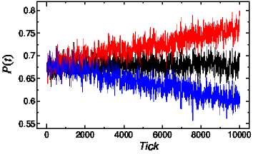
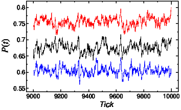
Figure 5: (Colour online) Monotonic increase and decrease trends generated by dealer model 92 with Eq. (6), where (b) is an enlargement of (a). $\varepsilon_{b}=-0.002$ for a monotonic increase trend, $\varepsilon_{b}=0.002$ for a monotonic decrease trend, and $\varepsilon_{s}=0$ for both the cases. The data with no trend is the same as that shown in Fig. 4(a). We show it for the for comparison. All other conditions are the same in Fig. 4.

Figure 5 is the data generated by the dealer model 92 with Eq. (6) instead of Eq. (3) where $\varepsilon_{b}=\pm 0.002$ and $\varepsilon_{s}=0$. We find a monotonically increasing trend for $\varepsilon_{b}=-0.002$ and a monotonically decreasing trend for $\varepsilon_{b}=0.002$ on Fig. 5(a). It should be noted that, as these monotonically increasing and decreasing trends are very slow, we cannot recognize the trends clearly if we take shorter period of time for observation, as is shown in Fig. 5(b). We have also confirmed that the dealer model 92 with $(\varepsilon_{b},\varepsilon_{s})=(0,0.002)$ show similar behaviours. Although the values of the parameters are small, this tiny little ulterior motive generates major trends. The results indicate that the trends are built on a delicate balance of acquisitive natures between the buyers and sellers. The results also indicate that, even if the amount of a change in the psychological tendency of a dealer is very small, it can bring a major influence on the market prices.

When we use larger values of $\varepsilon_{b}$ or $\varepsilon_{s}$ or when we use the pair of $\varepsilon_{b}$ and $\varepsilon_{s}$ together, we have confirmed to obtain steeper trends.

3.2 Trends with no supposition: unpremeditated trends

In the previous section we have confirmed that monotonic trends emerge by dealers’ expectation of the forthcoming price change, even if it is minuscule. In this case we can guess or estimate the underlying expectation of individual dealers based on their behaviours. In numerical calculations, we can obtain complete information about all deals. It should be emphasized, however, that it is almost impossible to acquire complete information in actual deals. In this section, we focus on the case in which only incomplete information on the deals is available and the influence of fundamentals and technical analyses on financial markets are almost absent.

Let us carefully examine an important feature of the dealer model 92. Generally speaking, it is impossible that all dealers in actual financial markets exactly know the number of sellers in every deal in advance. However, the number of sellers $n$ is included in Eq. (3) to reflect the acquisitive nature of the dealers. That is, the dealer model 92 contains a parameter which is impossible to know in advance in actual deals, though this parameter $n$ plays a crucial role in the model. As Eq. (3) shows, the buyer’s price falls $\delta$ and each of $n$ sellers’ prices rises $\delta/n$ when a deal is done. In other words, the total amount of the rises of the sellers’ prices $n\times\delta/n$ exactly compensates for the decline of the buyer’s price $\delta$. Because of this exact compensation effect, the price data generated by the dealer model 92 with Eq. (3) have only short-term variabilities and do not have trends.

It is unlikely and unnatural for sellers to know the precise number of sellers in any deal in advance (no dealer actually knows it). However, it is possible to know the number of sellers in the past deals. Let us examine the behaviours of the number of sellers of the data shown in Fig. 4. Figure 6 shows that the number of sellers varies wildly at each deal, where the minimum is 1 and the maximum is 14. It does not seem to be easy to predict the next number of sellers using the past data. In such cases each seller would have no other choice than to obey his/her own guess for the next price change. As a result, the expectation for buying and selling would not always cancel out. To formulate this situation simply, we use the average seller number $\mu_{n}(t)$ instead of the precise seller number $n$ in Eq. (3), where $\mu_{n}(t)$ is calculated using all of the seller number prior to time $t$ (that is, from $1$ to $t-1$). We note that this idea is not so irrelevant. When the prediction of the future value does not seem to be easy, one of the common approaches is to use the mean of the past values: the average number of sellers who participated deals in the past. Based on these considerations, Eq. (3) is modified as follows:

$$\Delta_{i}=\begin{cases}-\delta&\text{(for the buyer)},\\ \delta/\mu_{n}(t)&\text{(for the sellers)},\\ 0&\text{(for the nonparticipants of the deal)},\end{cases}$$ (7)

where $0<\delta<L$.

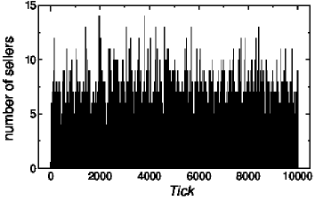
(a)

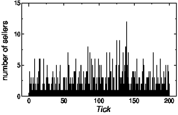
(b)

Figure 6: The number of sellers of Fig. 4. The data is generated by dealer model 92 of of Eq. (5). Plot (b) is an enlargement of (a). All other conditions are the same in Fig. 4.

Figure 7 shows the behaviours of the dealer models 92 with the modification by Eq. (7), where the average sellers number is used instead of the precise sellers number. Figure 7(a) shows that the simulated price data $P(t)$ have short-term variabilities and exhibit the appearance of long-term rising and falling behaviours of trends. The difference in the behaviour from the one for the original dealer model 92 shown in Fig. 4 due to the simple modification from $n$ to $\mu_{n}(t)$ in the definition of $\Delta_{i}$ is striking. The overall behaviour seems to be similar to the real data shown in Fig. 1. The original dealer model 92 with Eq. (3) generates only behaviours without trends [4], as shown in Fig. 4. Although we do not input previously prepared trends and add any driving force term to generate trends forcibly to the model, a variety of trends emerge under the condition that complete information about deals cannot be obtained in advance. This result implies that the dealer model 92 intrinsically contains the ability to behaviour trends without adding any external terms. Figure 7(b) shows that the average number of sellers converges very quickly. In contrast, from Fig. 7(c) that shows the number of sellers at each deal, the number fluctuates wildly at each deal between 1 and 13. The behaviour is similar to Fig. 6(a). We emphasize that the emergence of the long-term monotonic increase and decrease of price change (that is, “trends”) from the dealer model 92 is rarely reported. In Fig. 7 we calculate $\mu_{n}(t)$ using all of the seller number data prior to the deal at $t$, although taking the average over all seller number is not essential. Averaging over the data in a certain interval, that is to say, the last 100 seller number data from $t-1$ to $t-100$, is equally permissible for generating trends.

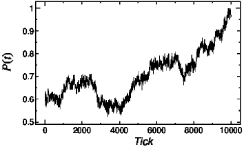
(a)

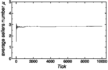
(b)

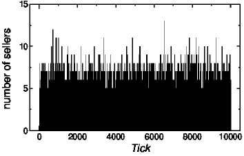
(c)

Figure 7: Typical behaviours of the dealer models 92 using the average number of sellers in the past. (a) simulated price data $P(t)$, (b) the average number of sellers, and (c) the number of sellers at each deal. All other parameter settings are the same in Fig. 4.

As mentioned above, the dealer model 92 with the present modification, Eq. (7), includes no driving force term to generate previously prepared trends. This result suggests that trends are not generated dynamically by external driving forces but emerge spontaneously from the aggregation of microscopic expectations of individual dealers.

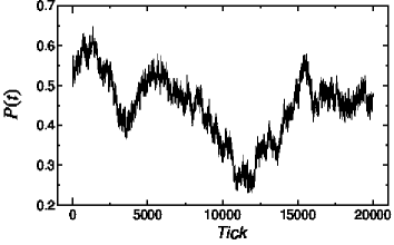
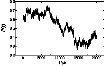
Figure 8: Different behaviours from that shown in Fig. 7(a), where different initial conditions of $B_{i}$ and different values of $a_{i}$ are used. All other parameter settings are the same in Fig. 7.

Figure 8 shows different behaviours from that shown in Fig. 7(a), where different initial conditions of $B_{i}$ and different values of $a_{i}$ are used. We find that there are short-term variabilities and trends in Figs. 8(a) and (b). We can also recognize a variety of movements such as upward, downward or sideways in Figs. 8(a) and (b). A trend in a long-term includes finer trends in shorter terms. For example, in Fig. 8(b) we recognize downward trends around the ticks between 7000 and 8500 and between 9000 and 11000, and an upward trend between 11000 and 12000. When we look at these price changes in a longer time scale, we recognize a downward trend around between 7000 and 15000. The overall downward trend thus contains these three short-term trends.

We also find another feature. One of the characteristic changes in the market price evolution is its sharp or abrupt change [4]. We find it around the ticks between 25500 and 26000 on Fig. 1(a) and between 24900 and 25500 on Fig. 1(b). We also find a similar sharp change on Fig. 8(b) between 13700 and 13800. It is remarkable that a little modification of the original dealer model 92 by Eq. (7) can produce such a variety of price changes exhibiting vital features seen in real financial markets.

3.3 Mingled trends with supposition and no supposition: premeditated trends and unpremeditated trends

In Section 3.1, we discussed an idea to generate monotonic increase and decrease trends. In Section 3.2, we discussed the emergence of trends due to the imbalance between the momentum of buying and selling because of incomplete information about the next deal. Although we discussed these two cases separately to make the arguments clear, they are strongly interconnected and mingled with each other in real financial markets. In this Section, therefore, we treat these two cases on the same footing.

Incorporating both ideas described in Sections 3.1 and 3.2, we adopt the following combined and improved modification for $\Delta_{i}$:

$$\Delta_{i}=\begin{cases}-\delta\times(1.0+\varepsilon_{b})&\text{(for the buyer)},\\ \delta/\mu_{n}(t)&\text{(for the sellers)},\\ 0&\text{(for nonparticipants of the deal)},\end{cases}$$ (8)

where the notations of $\delta$ and $n$ are the same as described in Eq. (3) and the notations of $\varepsilon_{b}$ and $\mu_{n}(t)$ as the same as described in Eqs. (6) and (7).

We generate price changes using the dealer model 92 with the modification Eq. (8) for different values of $\varepsilon_{b}$. The results show complicated and a wide variety of behaviours. Figure 9 shows one of the explicit results. We also show the plots for the data corresponding to unpremeditated trends defined by $\varepsilon_{b}=0$ for comparison. By replacing the number of sellers $n$ with the average value $\mu_{n}(t)$, the profiles of the trends becomes significantly susceptible to the actual values of $\varepsilon_{b}$. Without the replacement of $n$ with $\mu_{n}(t)$, a negative $\varepsilon_{b}$ generates a monotonically increasing trend, and a positive $\varepsilon_{b}$ generates a monotonically decreasing trend as shown in Fig. 5. Figure 9(a) shows similar results for $\varepsilon_{b}=\pm 0.031$. However, the sign of $\varepsilon_{b}$ does not have a simple relationship with increasing or decreasing nature of trends in this case. For Fig. 9(b), we use a much smaller absolute value for $|\varepsilon_{b}|=0.0021$ than that used in Fig. 9(a), $|\varepsilon_{b}|=0.031$. In this plot, a trend produced by the positive value, $\varepsilon_{b}=0.0021$, shows much more prominent increase than that produced by the negative value, $\varepsilon_{b}=-0.0021$. Only by taking a slightly smaller absolute value, $|\varepsilon_{b}|=0.002$, we see that a negative value, $\varepsilon_{b}=-0.002$, generates a decreasing trend and a positive value, $\varepsilon_{b}=0.002$, generates an increasing trend as shown in Fig. 9(c). Note that these values, $|\varepsilon_{b}|=0.002$, are the same as those used in Fig. 5.

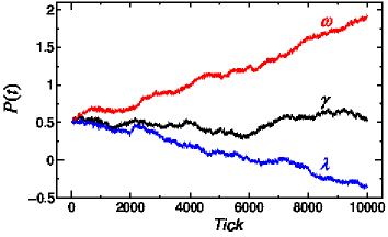
(a)

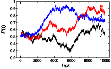
(b)

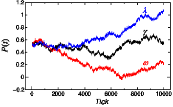
(c)

Figure 9: (Colour online) Mingled trends generated by the improved dealer model 92 defined by Eq. (8): (a) $\varepsilon_{b}=-0.031$ for plot $\omega$ and $\varepsilon_{b}=0.031$ for plot $\lambda$, (b) $\varepsilon_{b}=-0.0021$ for plot $\omega$ and $\varepsilon_{b}=0.0021$ for plot $\lambda$, (c) $\varepsilon_{b}=-0.002$ for plot $\omega$ and $\varepsilon_{b}=0.002$ for plot $\lambda$. All plots labelled by $\gamma$ in (a), (b), and (c) are the data generated by $\varepsilon_{b}=0$. Note that plot of $\omega$ originally corresponds to a monotonic increase trend, that of $\lambda$ to a monotonic decrease trend, and that of $\gamma$ to unpremeditated trends. All other conditions are the same in Fig. 4.

4 Discussions and Summary

When we use both ideas to generate trends with supposition and no supposition at the same time in Section 3.3, we observed two distinctive aspects. One is that dealers’ minuscule tendencies in next price setting can make a large difference in the overall behaviours of price change. The other is that there are cases where the behaviours of price change are different from, even opposite to, individual dealers’ expectations. Both of the aspects indicate that the direction of trends cannot tell us the underlying expectations of the dealers. In other words, the behaviours of the trend do not always accord with dealers’ long-term expectations. This leads to a very intriguing conclusion. From the behaviours or movements of price change, each dealer infers his/her specious justification of the cause of the change and offer future prospects to others in the next deal. Once the price in a market moves against their expectations, however, dealers doubt their justifications and may take a counter reaction to their original expectation. Such counter reactions of the dealers may cause excess volatility.

We understand that there might be other origins to generate trends than the ones described in this paper. The reason we believe that the origins discussed in the present paper are essential is their universality. As no dealer has access to complete information about the next deal in actual financial markets, dealers have no choice other than to have their own expectations. As these expectations are brought by incomplete information, the expectations would be rough and flimsy. Such flimsy expectations of individual dealers break a subtle balance of acquisitive natures between buyers and sellers and generate macroscopic trends, even if there are no external driving factors. Since the situations in which we cannot obtain complete information about the next status are very common, we believe that the knowledge gained from the ideas pursued in this paper contains an essential ingredient and can be applicable to many other situations For example, we often find the price changes in actual markets that exhibit very similar behaviours, although the brands are different, such as Australian Dollar/USD exchange rate and New Zealand Dollar/USD exchange rate.

Our results indicate that some trends might be unpremeditated. Although the trends emerge spontaneously, why their behaviours are so similar? What kind of interactions are there between the brands? Those will be very interesting future questions.

Summary of the results is the following. In this paper, we have investigated possible origins of trends in financial market price changes using a deterministic threshold model called the dealer model 92. We consider financial markets as a game field of commercial activity composed of human choices and their interactions. First, we have observed that monotonically increasing and decreasing trends can be generated by dealers’ minuscule tendencies for price setting according to the expected forthcoming price changes. Next, we have observed that irregular fluctuations with short-term variabilities and trends emerge spontaneously under the assumption that we cannot obtain complete information about the next deal in advance. In both cases, trends are generated without introducing any external driving forces to the original dealer modes 92. Finally, we have confirmed that the numerical data for price change generated by the dealer model 92 incorporating both of these two cases contains several vital features observed in real financial markets. These results indicates that emergence of trends might be inevitable in any realistic situations, even if the influence on fundamentals and technical analyses in financial markets is almost absent.

5 Acknowledgements

We would like to thank the anonymous referees for their very valuable remarks. One of the authors, TT, would like to acknowledge the support of Grant-in-Aid for Scientific Research (C) (No. 24540419) from the Japan Society for the Promotion of Science.

References

- [1] R. N. Mantegna, H. E. Stanley, Scaling behaviour in the dynamics of an economic index, Nature 376 (1995) 46–49.
- [2] T. Ohira, N. Sazuka, K. Marumo, T. Shimizu, M. Takayasu, H. Takayasu, Predictability of currency market exchange, Physica A 308 (2002) 368–374.
- [3] T. Nakamura, M. Small, Tests of the random walk hypothesis for financial data, Physica A 377 (2007) 599–615.
- [4] H. Takayasu, H. Miura, T. Hirabayashi, K. Hamada, Statistical properties of deterministic threshold elements - the case of market price, Physica A 184 (1992) 127–134.
- [5] A. Sato, H. Takayasu, Dynamic numerical models of stock market price: from microscopic determinism to macroscopic randomness, Physica A 250 (1998) 231–252.
- [6] F. Ren, B. Zheng, T. Qiu, S. Trimper, Minority games with score-dependent and agent-dependent payoffs, Phys. Rev. E 74 (2006) 041111.
- [7] T. Kaizoji, An interacting-agent model of financial markets from the viewpoint of nonextensive statistical mechanics, Physica A 370 (2006) 109–113.
- [8] J. Maskawa, Stock price fluctuations and the mimetic behaviors of traders, Physica A 382 (2007) 172–178.
- [9] V. Alfi, M. Cristelli, L. Pietronero, A. Zaccaria, Minimal agent based model for financial markets II: Statistical properties of the linear and multiplicative dynamics, The European Physical Journal B 67 (2009) 399–417.
- [10] K. Yamada, H. Takayasu, M. Takayasu, Characterization of foreign exchange market using the threshold-dealer-model, Physica A 382 (2007) 340–346.
- [11] K. Yamada, H. Takayasu, T. Ito, M. Takayasu, Solvable stochastic dealer models for financial markets, Phys. Rev. E 79 (2009) 051120.
- [12] T. Hirabayashi, H. Takayasu, H. Miura, K. Hamada, The behavior of a threshold model of market price in stock exchange, Fractals 1 (1993) 29–40.
- [13] T. Nakamura, M. Small, Small-shuffle surrogate data: Testing for dynamics in fluctuating data with trends, Phys. Rev. E 72 (2005) 056216.