Bounds on Eigenvalues of a Spatial Correlation Matrix

Abstract

It is critical to understand the properties of spatial correlation matrices in massive multiple-input multiple-output (MIMO) systems. We derive new bounds on the extreme eigenvalues of a spatial correlation matrix that is characterized by the exponential model in this paper. The new upper bound on the maximum eigenvalue is tighter than the previous known bound. Moreover, numerical studies show that our new lower bound on the maximum eigenvalue is close to the true maximum eigenvalue in most cases. We also derive an upper bound on the minimum eigenvalue that is also tight. These bounds can be exploited to analyze many wireless communication scenarios including uniform planar arrays, which are expected to be widely used for massive MIMO systems.

I Introduction

Spatial correlation in the channel can give both gains and losses depending on the scenario in multiple-input multiple-output (MIMO) systems [1]. Spatial correlation is harmful for single-user MIMO systems using multiplexing because the correlation reduces the rank of the communication channel, resulting in a reduced number of parallel paths for spatial multiplexing [2]. On the other hand, spatial correlation is beneficial for multi-user MIMO systems because the strong directivity of channels between a transmitter and users can help to reduce inter-user interference even with simple precoding strategies at the transmitter [1].

The most common model for the spatial correlation matrix is the exponential model [1, 3]. The exponential model is very simple because the correlation matrix is controlled by one parameter. Although simple, it has been shown experimentally that the exponential model characterizes uniform linear array (ULA) antenna scenarios well [3]. Thus, many works, e.g., capacity analyses in [4, 5], codebook designs for channel state information (CSI) quantization in [6, 7, 8], and training signal designs for channel estimation in [9, 10, 11], are based on the exponential model for the spatial correlation matrix.

The exponential model is useful for analyzing uniform planar array (UPA) scenarios. Note that UPA deployments are growing in popularity due to the emergence of massive MIMO systems [12, 13]. It was shown in [14] that the spatial correlation matrix of a UPA can be approximated by the Kronecker product of the spatial correlation matrices corresponding to the vertical and horizontal domain. In [15, 14], this approximation was exploited to design codebooks for CSI quantization in a UPA scenario.

Because of the reasons above, we focus on spatial correlation matrices following the exponential model in this paper. The maximum and minimum eigenvalues of the spatial correlation matrix are important factors because they determine performance in spatially correlated channels [16, 17]. In this paper, we derive new upper and lower bounds on the maximum eigenvalue and an upper bound on the minimum eigenvalue of the correlation matrix. Although the exact eigenvalues of the exponential model are derived in [18], the expressions need numerical solutions of the trigonometric function. Moreover, the bounds derived from the exact expressions are not functions of the number of transmit antennas, which makes it hard to analyze massive MIMO systems with practical numbers of antennas. Thus, it is desired to have simple and tight upper and lower bounds on extreme eigenvalues expressed with the number of antennas for analyzing the exponential model.

The new upper bound on the maximum eigenvalue, which is based on a novel matrix expansion approach, is tighter than the one from [18]. Moreover, simulation results show that our lower bound on the maximum eigenvalue is very tight with the true value in general. The new upper bound on the minimum eigenvalue is tight as well. All these new bounds are functions of the number of transmit antennas. The new lower bound on the maximum eigenvalue and upper bound on the minimum eigenvalue are intuitive and simple to be derived; however, we could not find such derivations even after extensive literature search. Most of the literature adopted the previous bounds in [18] for performance analysis [4, 11] or simply performed numerical studies with the exponential model [5, 6, 7, 8, 9, 10].

II System Model

We consider multiple-input single-output (MISO) channels that are spatially correlated at the transmitter side. Assuming $N_{t}$ transmit antennas at the transmitter, the input-output relation at baseband is given as

$$y={\mathbf{h}}^{H}{\mathbf{x}}+n,$$

where $y$ is the received signal, ${\mathbf{h}}\in\mathbb{C}^{N_{t}}$ is the channel vector, ${\mathbf{x}}\in\mathbb{C}^{N_{t}}$ is the transmitted signal, and $n\sim{\mathcal{C}}{\mathcal{N}}(0,\sigma^{2})$ is additive complex Gaussian noise. Because we consider spatially correlated channels, ${\mathbf{h}}$ is modeled as

$${\mathbf{h}}={\mathbf{R}}^{\frac{1}{2}}{\mathbf{h}}_{w}$$

where ${\mathbf{R}}=E[{\mathbf{h}}{\mathbf{h}}^{H}]$ is the spatial correlation matrix and ${\mathbf{h}}_{w}\sim{\mathcal{C}}{\mathcal{N}}(\mathbf{0},{\mathbf{I}}_{N_{t}})$ is an i.i.d. complex Gaussian vector.

Depending on antenna structure, ${\mathbf{R}}$ can be modeled in many ways. There is particular interest of antenna deployments using UPAs in massive MIMO systems. Note that a UPA can support a large number of antennas compactly, which makes massive MIMO practical. For a UPA, [14] showed by eigenvalue and capacity distributions that the spatial correlation matrix of a UPA can be approximated as

$${\mathbf{R}}\approx{\mathbf{R}}_{h}\otimes{\mathbf{R}}_{v}$$ (1)

where $\otimes$ is the Kronecker product and ${\mathbf{R}}_{v}$ and ${\mathbf{R}}_{h}$ are the spatial correlation matrices of the horizontal and vertical domains, respectively.

The simplified model in (1) makes it possible to adopt any kind of ULA spatial correlation model for ${\mathbf{R}}_{h}$ and ${\mathbf{R}}_{v}$ because a UPA is simply a ULA in each vertical and horizontal domain (assuming co-polarized antennas). Therefore, it is important to understand the spatial correlation matrix properties of a ULA to understand those of a UPA.

Note that the maximum and minimum eigenvalues of ${\mathbf{R}}$ are particularly important in analyzing spatially correlated channels [16, 17]. From (1), we have

$${\mathbf{R}} \approx{\mathbf{R}}_{h}\otimes{\mathbf{R}}_{v}$$

$$=\left({\mathbf{U}}_{h}\mathbf{\Lambda}_{h}{\mathbf{U}}_{h}^{H}\right)\otimes\left({\mathbf{U}}_{v}\mathbf{\Lambda}_{v}{\mathbf{U}}_{v}^{H}\right)$$

$$=\left({\mathbf{U}}_{h}\otimes{\mathbf{U}}_{v}\right)\left(\mathbf{\Lambda}_{h}\otimes\mathbf{\Lambda}_{v}\right)\left({\mathbf{U}}_{h}\otimes{\mathbf{U}}_{v}\right)^{H}$$

where ${\mathbf{R}}_{h}={\mathbf{U}}_{h}\mathbf{\Lambda}_{h}{\mathbf{U}}_{h}^{H}$ and ${\mathbf{R}}_{v}={\mathbf{U}}_{v}\mathbf{\Lambda}_{v}{\mathbf{U}}_{v}^{H}$ denote the eigen-decompositions. Let $\lambda_{k}({\mathbf{A}})$ be the $k$-th largest eigenvalue of the matrix ${\mathbf{A}}$. Then, we have

$$\lambda_{1}({\mathbf{R}})\approx\lambda_{1}({\mathbf{R}}_{h})\lambda_{1}({\mathbf{R}}_{v}),\quad\lambda_{N_{t}}({\mathbf{R}})\approx\lambda_{N_{t}}({\mathbf{R}}_{h})\lambda_{N_{t}}({\mathbf{R}}_{v}).$$ (2)

For these reasons, we focus on the spatial correlation matrix of a ULA in this paper.

We let ${\mathbf{R}}$ denote a ULA spatial correlation matrix. There are many ways to model ${\mathbf{R}}$ depending on scenario. The most common and easy way to model ${\mathbf{R}}$ is to rely on the exponential model which is given as

$${\mathbf{R}}_{[i,j]}=\begin{cases}r^{|i-j|}&\quad\text{if }i\geq j\\ (r^{*})^{|i-j|}&\quad\text{if }i<j\end{cases}$$ (3)

where ^∗ denotes a complex conjugate, $r=ae^{j\theta}$ is the correlation coefficient of ${\mathbf{R}}$ with $0\leq a<1$. Note that the eigenvalues of ${\mathbf{R}}$ only depend on the value of $a$, and $\theta$ only controls the eigenvectors of ${\mathbf{R}}$. Because we are interested in the maximum and minimum eigenvalues of ${\mathbf{R}}$, we assume $r=a$ throughout the paper.

III Bounds on Eigenvalues

We first briefly recall previous results on analyzing the eigenvalues of ${\mathbf{R}}$. We then derive new bounds on the maximum and minimum eigenvalues of ${\mathbf{R}}$.

III-A Previous Results

In [18], it has been shown that all eigenvalues of ${\mathbf{R}}$ can be exactly derived as

$$\lambda_{i}({\mathbf{R}})=\frac{1-a^{2}}{1+a^{2}+2a\cos\phi_{i}}$$ (4)

where $\phi_{i}\neq n\pi$ for any arbitrary integer $n$ are the solutions of the trigonometric equation

$$\tan N_{t}\phi_{i}=\frac{-\sin\phi_{i}}{\left(\frac{1+a^{2}}{1-a^{2}}\right)\cos\phi_{i}+\frac{2a}{1-a^{2}}}.$$

From (4), it is obvious that

$$\lambda_{1}({\mathbf{R}}) \leq\frac{1+a}{1-a},$$ (5)

$$\lambda_{N_{t}}({\mathbf{R}}) \geq\frac{1-a}{1+a}.$$ (6)

Remark: Note that the bounds in (5) and (6) are not functions of the number of antennas $N_{t}$. Thus, it is not clear how the extreme eigenvalues would behave as $N_{t}$ grows large, which is an important aspect in predicting performance of massive MIMO systems [19].

III-B New Bounds on Eigenvalues

In the following, we derive an improved upper bound and new lower bound on $\lambda_{1}({\mathbf{R}})$ that are both functions of $N_{t}$.

Lemma 1.

With the exponential model of ${\mathbf{R}}$ as in (3), the maximum eigenvalue of ${\mathbf{R}}$ is bounded as

$$\frac{1+a}{1-a}-\frac{2a(1-a^{N_{t}})}{N_{t}(1-a)^{2}}\leq\lambda_{1}({\mathbf{R}})\leq\frac{(1+a)(1-a^{N_{t}-1})}{1-a}$$

when $N_{t}>1$.

Proof:

We first prove the upper bound. We extend ${\mathbf{R}}$ to an $2(N_{t}-1)\times 2(N_{t}-1)$ circulant matrix as

$${\mathbf{R}}_{X}=\begin{bmatrix}1&a&\cdots&a^{N_{t}-1}&a^{N_{t}-2}&a^{N_{t}-3}&\cdots&a\\ a&1&\cdots&a^{N_{t}-2}&a^{N_{t}-1}&a^{N_{t}-2}&\cdots&a^{2}\\ \vdots&\vdots&\cdots&&\ddots&&&\vdots\\ a&a^{2}&\cdots&a^{N_{t}-2}&a^{N_{t}-3}&a^{N_{t}-4}&\cdots&1\end{bmatrix}.$$

Note that ${\mathbf{R}}$ is contained in the first $N_{t}$ rows and $N_{t}$ columns of ${\mathbf{R}}_{X}$. Therefore,

$$\lambda_{1}({\mathbf{R}})\leq\lambda_{1}({\mathbf{R}}_{X}).$$

Because ${\mathbf{R}}_{X}$ is a circulant matrix, the eigenvectors of ${\mathbf{R}}_{X}$ are the columns of the $2(N_{t}-1)$ point DFT matrix. If we let $\mathbf{1}_{N}$ be the $N\times 1$ vector with all one entries, it is easy to conclude that the dominant eigenvector of ${\mathbf{R}}_{X}$ is

$${\mathbf{u}}_{1}({\mathbf{R}}_{X})=\frac{1}{\sqrt{2(N_{t}-1)}}\mathbf{1}_{2(N_{t}-1)}$$

that cophases all of the entries of ${\mathbf{R}}_{X}$ because of the assumption that $a$ is a real positive number. Then, we have

$$\lambda_{1}({\mathbf{R}}_{X}) ={\mathbf{u}}_{1}({\mathbf{R}}_{X})^{H}{\mathbf{R}}_{X}{\mathbf{u}}_{1}({\mathbf{R}}_{X})$$

$$=\frac{1}{2(N_{t}-1)}\sum_{k=1}^{2(N_{t}-1)}\left(\sum_{\ell_{1}=0}^{N_{t}-1}a^{\ell_{1}}+\sum_{\ell_{2}=1}^{N_{t}-2}a^{\ell_{2}}\right)$$

$$=\frac{(1+a)(1-a^{N_{t}-1})}{1-a}.$$

Thus,

$$\lambda_{1}({\mathbf{R}})\leq\lambda_{1}({\mathbf{R}}_{X})=\frac{(1+a)(1-a^{N_{t}-1})}{1-a}.$$

To prove the lower bound, we use the definition of the maximum eigenvalue, which follows the general inequality

$$\lambda_{1}({\mathbf{R}})\geq{\mathbf{f}}^{H}{\mathbf{R}}{\mathbf{f}}$$

with an arbitrary vector ${\mathbf{f}}$ satisfying $\|{\mathbf{f}}\|_{2}^{2}=1$. Because the elements of ${\mathbf{R}}$ are all positive real numbers, the all one vector $\mathbf{1}_{N_{t}}$ with appropriate normalization would give a good lower bound on $\lambda_{1}({\mathbf{R}})$. Thus, we have

$$\lambda_{1}({\mathbf{R}}) \geq\frac{1}{N_{t}}\mathbf{1}_{N_{t}}^{T}{\mathbf{R}}\mathbf{1}_{N_{t}}$$

$$=\frac{1}{N_{t}}\left(2\sum_{\ell=0}^{N_{t}-1}\sum_{k=0}^{\ell}a^{k}-N_{t}\right)$$

$$=\frac{1+a}{1-a}-\frac{2a(1-a^{N_{t}})}{N_{t}(1-a)^{2}}$$

which finishes the proof. ∎

It is obvious that the upper bound in Lemma 1 improves on (5) because

$$\frac{(1+a)(1-a^{N_{t}-1})}{1-a}\leq\frac{1+a}{1-a}$$

for arbitrary $0\leq a<1$. Moreover, the upper and lower bounds on $\lambda_{1}({\mathbf{R}})$ both converge to (5) as $N_{t}\rightarrow\infty$. This shows that all three bounds become tight when $N_{t}$ is large.

It is also interesting to analyze the tightness of the upper and lower bounds on $\lambda_{1}({\mathbf{R}})$ regarding $a$. Let $\lambda_{1}^{\mathrm{diff}}({\mathbf{R}})$ be the difference of the two bounds in Lemma 1, which is given as

$$\lambda_{1}^{\mathrm{diff}}({\mathbf{R}})=\frac{(1+a)(1-a^{N_{t}-1})}{1-a}-\left(\frac{1+a}{1-a}-\frac{2a(1-a^{N_{t}})}{N_{t}(1-a)^{2}}\right).$$

With some algebra, we can show that $\lambda_{1}^{\mathrm{diff}}({\mathbf{R}})$ is monotonically increasing with $a$. Moreover, $\lambda_{1}^{\mathrm{diff}}({\mathbf{R}})\rightarrow 0$ as $a\rightarrow 0$ and $\lambda_{1}^{\mathrm{diff}}({\mathbf{R}})\rightarrow N_{t}-2$ as $a\rightarrow 1$. Thus, the two bounds are tight when $a$ is small while the gap becomes large as $a$ increases. This is verified numerically in Section IV.

Now, we derive an upper bound on the minimum eigenvalue of ${\mathbf{R}}$. The numerical studies in Section IV show that the lower bound in (6) and the new upper bound on $\lambda_{N_{t}}({\mathbf{R}})$ are both tight in general.

Lemma 2.

With the exponential model of ${\mathbf{R}}$ as in (3), the minimum eigenvalue of ${\mathbf{R}}$ is upper bounded as

$$\lambda_{N_{t}}({\mathbf{R}})\leq\frac{1-a}{1+a}+\frac{2a(1-(-a)^{N_{t}})}{N_{t}(1+a)^{2}}$$

Proof:

We only prove when $N_{t}$ is even. Similar derivation can be shown when $N_{t}$ is odd. Using the definition of the minimum eigenvalue, we have the general inequality

$$\lambda_{N_{t}}({\mathbf{R}})\leq{\mathbf{f}}^{H}{\mathbf{R}}{\mathbf{f}}$$

for an arbitrary vector ${\mathbf{f}}$ with $\|{\mathbf{f}}\|_{2}^{2}=1$. Let $\tilde{\mathbf{1}}_{N}$ be the $N\times 1$ vector defined as

$$\tilde{\mathbf{1}}_{N}=\begin{bmatrix}1,-1,1,-1\cdots,(-1)^{N-2},(-1)^{N-1}\end{bmatrix}^{T}.$$

We can upper bound $\lambda_{N_{t}}({\mathbf{R}})$ with $\tilde{\mathbf{1}}_{N_{t}}$ as

$$\lambda_{N_{t}}({\mathbf{R}})\leq\frac{1}{N_{t}}\tilde{\mathbf{1}}_{N_{t}}^{T}{\mathbf{R}}\tilde{\mathbf{1}}_{N_{t}}$$

$$=1-\frac{2}{N_{t}}\left(\sum_{k=1}^{\frac{N_{t}}{2}}\left(N_{t}-(2k-1)\right)a^{2k-1}\sum_{k=1}^{\frac{N_{t}}{2}-1}\left(N_{t}-2k\right)a^{2k}\right).$$

We can get the desired result after solving the above series and employing basic algebra. ∎

Using these bounds, we can also derive upper and lower bounds on the condition number of ${\mathbf{R}}$ and on the (approximated) maximum and minimum eigenvalues of UPA spatial correlation matrix by (2).

IV Numerical Studies

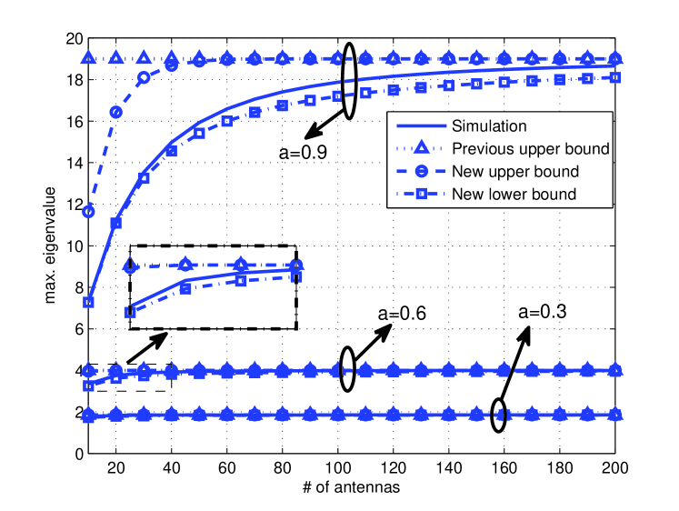
Figure 1: The plots of $\lambda_{1}({\mathbf{R}})$ and its upper and lower bounds according to $N_{t}$. The previous upper bound is from (5) and the new upper and lower bounds are based on Lemma 1.

First, we plot the maximum eigenvalue of ${\mathbf{R}}$, $\lambda_{1}({\mathbf{R}})$, and the upper and lower bounds from (5) and Lemma 1 according to the number of antennas $N_{t}$ in Fig. 1. The new upper bound derived in Lemma 1 is tight when $a$ is low to moderate, while the gap between the new upper bound and the true $\lambda_{1}({\mathbf{R}})$ becomes large when $a=0.9$. However, the new upper bound keeps following the curve of $\lambda_{1}({\mathbf{R}})$ while the previous upper bound in (5) is constant regardless of $N_{t}$. It is interesting to point out that the new lower bound is tight for all values of $N_{t}$ and $a$. Therefore, the new lower bound can be used as an excellent approximation of $\lambda_{1}({\mathbf{R}})$. As mentioned earlier, the upper and lower bounds in Lemma 1 are tight when $a$ is low to moderate, and the gap becomes large as $a$ approaches one.

In Fig. 2, we plot the minimum eigenvalue $\lambda_{N_{t}}({\mathbf{R}})$, the new upper bound from Lemma 2, and the previous lower bound in (6) with $N_{t}$. Regarding the minimum eigenvalue, the two bounds are both tight regardless of the values of $a$ and $N_{t}$.

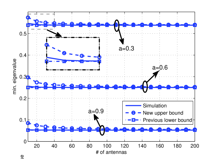
Figure 2: The plots of $\lambda_{N_{t}}({\mathbf{R}})$, the previous lower bound from (6) and the new upper bound from Lemma 2 according to $N_{t}$.

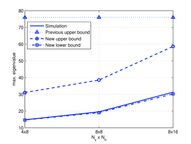
Figure 3: The plots of $\lambda_{1}({\mathbf{R}})$ for the UPA scenario and its upper and lower bounds with different numbers of $N_{h}$ and $N_{v}$. The correlation coefficients of ${\mathbf{R}}_{v}$ and ${\mathbf{R}}_{h}$ are set to $0.6$ and $0.9$, respectively.

Finally, we plot the maximum eigenvalue of the spatial correlation matrix of UPA given in (1) and its upper and lower bounds with different combinations of the numbers of vertical and horizontal domain antennas in Fig. 3. All bounds are based on the approximations (2) and derived as in the case of Fig. 1. We set the correlation coefficient of ${\mathbf{R}}_{h}$ as 0.6 and that of ${\mathbf{R}}_{v}$ as 0.9. It is clear that the new lower bound is very tight for all antenna combinations. The new upper bound also gives much better tightness compared to the previous upper bound.

V Conclusion

In this paper, we derived new bounds on the maximum and minimum eigenvalues of a spatial correlation matrix that is characterized by the exponential model. The upper bound on the maximum eigenvalue derived in this paper gives improved tightness than the previous upper bound. Moreover, using numerical studies, the new lower bound on the maximum eigenvalue is shown to be very tight regardless of the number of antennas and the intensity of spatial correlation. We also derived a new upper bound on the minimum eigenvalue of the spatial correlation matrix. It was shown by simulations that the new upper bound and the previous lower bound on the minimum eigenvalue are both tight in general. The theoretical results derived in this paper can be applied to performance analyses in many wireless communication scenarios including uniform planar array, which are growing in popularity due to the emergence of massive MIMO systems.

References

- [1] B. Clerckx, G. Kim, and S. Kim, “Correlated fading in broadcast MIMO channels: curse or blessing?” Proceedings of IEEE Global Telecommunications Conference, Dec. 2008.
- [2] H. Shin and J. Lee, “Capacity of multiple-antenna fading channels: spatial fading correlation, double scattering, and keyhole,” IEEE Transactions on Information Theory, vol. 49, no. 10, pp. 2636–2647, Oct. 2003.
- [3] B. T. Maharaj, J. W. Wallace, L. P. Linde, and M. A. Jensen, “Frequency scaling of spatial correlation from co-located 2.4 and 5.2GHz wideband indoor MIMO channel measurements,” Electronic Letters, vol. 41, no. 6, pp. 336–337, Mar. 2005.
- [4] X. Mestre, J. R. Fonollosa, and A. Pagès-Zamora, “Capacity of MIMO channels: asymptotic evaluation under correlated fading,” IEEE Journal on Selected Areas in Communications, vol. 21, no. 5, pp. 829–838, Jun. 2003.
- [5] S. L. Loyka, “Channel capacity of MIMO architecture using the exponential correlation matrix,” IEEE Communications Letters, vol. 5, no. 9, pp. 369–371, Sep. 2001.
- [6] J. Choi, B. Clerckx, N. Lee, and G. Kim, “A new design of polar-cap differential codebook for temporally/spatially correlated MISO channels,” IEEE Transactions on Wireless Communications, vol. 11, no. 2, pp. 703–711, Feb. 2012.
- [7] B. Clerckx, G. Kim, and S. Kim, “MU-MIMO with channel statistics-based codebooks in spatially correlated channel,” Proceedings of IEEE Global Telecommunications Conference, Dec. 2008.
- [8] J. Choi, V. Raghavan, and D. J. Love, “Limited feedback design for the spatially correlated multi-antenna broadcast channel,” Proceedings of IEEE Global Telecommunications Conference, Dec. 2013.
- [9] J. H. Kotecha and A. M. Sayeed, “Transmit signal design for optimal estimation of correlated MIMO channels,” IEEE Transaction on Signal Processing, vol. 52, pp. 546–557, Feb. 2004.
- [10] E. Björnson and B. Ottersten, “A framework for training-based estimation in arbitrarily correlated Rician MIMO channels with Rician distrubance,” IEEE Transaction on Signal Processing, vol. 58, no. 3, pp. 1807–1820, Mar. 2010.
- [11] J. Choi, D. J. Love, and P. Bidigare, “Downlink training techniques for FDD massive MIMO systems: open-loop and closed-loop training with memory,” IEEE Journal of Selected Topics in Signal Processing, to appear.
- [12] F. Rusek, D. Persson, B. K. Lau, E. G. Larsson, T. L. Marzetta, O. Edfors, and F. Tufvesson, “Scaling up MIMO: opportunities and challenges with very large arrays,” IEEE Signal Processing Magazine, vol. 30, no. 1, pp. 40–60, Jan. 2013.
- [13] Y. Nam, B. L. Ng, K. Sayana, Y. Li, J. Zhang, Y. Kim, and J. Lee, “Full-dimension MIMO (FD-MIMO) for next generation cellular technology,” IEEE Communications Magazine, vol. 51, no. 6, pp. 172–179, Jun. 2013.
- [14] D. Ying, F. W. Vook, T. A. Thomas, D. J. Love, and A. Ghosh, “Kronecker product correlation model and limited feedback codebook design in a 3D channel model,” Proceedings of IEEE International Conference on Communications, Jun. 2014.
- [15] J. Li, X. Su, J. Zeng, Y. Zhao, S. Yu, L. Xiao, and X. Xu, “Codebook design for uniform rectangular arrays of massive antennas,” Proceedings of IEEE Vehicular Technology Conference, Jun. 2013.
- [16] V. Raghavan, S. V. Hanly, and V. V. Veeravalli, “Statistical beamforming on the Grassmann manifold for the two-user broadcast channel,” IEEE Transactions on Information Theory, vol. 59, no. 10, pp. 6464–6489, Oct. 2013.
- [17] V. Raghavan and V. V. Veeravalli, “Ensemble properties of RVQ-based limited-feedback beamforming codebooks,” IEEE Transactions on Information Theory, vol. 59, no. 12, pp. 8224–8249, Dec. 2013.
- [18] J. N. Pierce and S. Stein, “Multiple diversity with nonindependent fading,” Proceedings of the IRE, vol. 48, no. 1, pp. 89–104, Jan. 1960.
- [19] A. Muller, A. Kammounz, E. Björnson, and M. Debbah, “Efficient linear precoding for massive MIMO systems using truncated polynomial expansion,” IEEE Sensor Array and Multichannel Signal Processing Workshop, to appear.