Constructing directed networks from multivariate time series using linear modelling technique

Abstract

We describe a method to construct directed networks from multivariate time series which has several advantages over the widely accepted methods. This method is based on an information theoretic reduction of linear (auto-regressive) models. The models are called reduced auto-regressive (RAR) models. The procedure of the proposed method is composed of three steps: (i) each time series is treated as a basic node of a network, (ii) multivariate RAR models are built and the constituent information in the models is summarized, and (iii) nodes are connected with a directed link based on that summary information. The proposed method is demonstrated for numerical data generated by known systems, and applied to several actual time series of special interest. Although the proposed method can identify connectivity, there are three points to keep in mind: (1) the proposed method cannot always identify nonlinear relationships among components, (2) as constructing RAR models is NP-hard, the network constructed by the proposed method might be near-optimal network when we cannot perform an exhaustive search, and (3) it is difficult to construct appropriate networks when the observational noise is large.

1 Introduction

Time series of natural phenomena usually show irregular fluctuations, and it is often found that such behaviours can be attributed to time delays (periodicities) in systems [1]. We consider periodicities as an important clue to understand dynamical phenomena in nature, irrespective of whether the data are linear or nonlinear. When data is linear the information of periodicities is directly linked to essential understanding of the linear system generating the data. Nonlinear data might also have periodicities. In this case the periodicities is one of the important clues to understand the underlying characteristic in the data and the system. In this paper, we propose a method to construct directed networks from multivariate time series from the perspective of linear periodic structures (relationships).

There has been various works for constructing networks from multivariate time series and many applications [2, 3, 4, 5, 6, 7, 8, 9, 10, 11, 12, 13, 14]. Among them, there are two previously proposed and widely accepted approaches for constructing networks from multivariate time series. One uses information from the frequency domain in which phase differences (shifts or delays) at a frequency between two signals are examined [7], and the other uses information from the time domain in which similarities between two signals are examined in terms of time differences [12].

Although both approaches have proven to be effective in various cases [7, 12], we feel that their effectiveness is constrained by the following two possible concerns. The first one is that, as the perspective to construct the networks by these approaches has never been clearly specified, what the constructed networks actually represent is not clear. In these approaches, multivariate auto-regressive (MVAR) model, the cross correlation (CC) function, and a fixed threshold value are applied to investigate the existence of relationship between a pair of time series [7, 12]. The second concern is that these statistical approaches often cannot adequately capture more local, nonlinear, or non-stationary peculiarities of time series. As a result, it is not clear what the constructed networks by the methods indicate for the data. Although the perspective of these approaches has never been clearly specified, we consider that the perspective of these approaches corresponds to linear periodic structures, because the MVAR model and the CC function are used. As mentioned above, both approaches are indirect methods to identify underlying linear periodic structures among multivariate time series. We consider that more straightforward approach is preferable to identify subtle features of the structures.

In this paper we propose a method which can construct networks from multivariate time series reflecting their dynamical nature as faithfully as possible based on a firm perspective. The proposed method utilizes a previously proposed linear model, the reduced auto-regressive (RAR) model [15, 16, 17]. The RAR model can precisely identify periodicities that are present in a time series, irrespective of whether the data is linear or nonlinear, provided the time series is sufficiently long [17]. Of course, there are restrictions when applying the proposed method. The RAR model cannot always identify nonlinear periodic structure in the data. To build a RAR model we need to find the optimal subset of possible terms for the model, which is expected to be an NP-hard problem. In this case, we usually use a selection algorithm, and the obtained RAR model might be only nearly optimal. It is also difficult to build appropriate RAR models (and to construct appropriate networks) when the observational noise is large.

The paper is organized as follows. We briefly review two widely accepted approaches as the current approaches in Section 2. In Section 3 we identify the network we like to construct from a given set of time series. In Section 4 we describe the problems with the current approaches, and show that the current approaches cannot construct the desired networks. In Sections 5 and 6 we introduce our method and apply the proposed method to several cases using simulated multivariate time series of known linear systems where there are correct linear model systems and the Rössler systems where there is no correct linear system. We discuss difficulties with building RAR models in Section 7. In Section 8 we apply our method to real-world multivariate time series data, which are meteorological data and electroencephalography data.

2 Current approaches

There are two major approaches to construct networks from multivariate time series, which are classified into the frequency-based approach and the time-based approach. In these approaches each individual time series is treated as a basic node of a network and a threshold is used to test the existence of relationship between data.

2.1 Frequency-based approach to network construction

There are also two widely accepted frequency-based methods [7, 18, 19]. One is Directed Transfer Function (DTF) [2, 3], and the other is Partial Directed Coherence (PDC) [4]. DTF was proposed as a multivariate spectral measure to determine the directional influences between any given pair of time series in a multivariate dataset [2, 3]. DTF is an estimator that simultaneously characterizes the direction and spectral properties of the interaction between signals. PDC was proposed as a factorization of the Partial Coherence after DTF, and PDC is based on MVAR coefficients transformed into the frequency domain [4]. Both methods are based on the MVAR model, and the MVAR model is transformed to the frequency domain by the Fourier transform (or $z$ transformation) to investigate the spectral properties. The pair of nodes corresponding to the chosen two time series is connected with a directed link when a value calculated by both the methods is larger than an appropriately chosen threshold. A threshold value is used to determine whether the values are large enough. See more details on DTF and PDC elsewhere [2, 3, 4, 7].

Both DTF and PDC are based on the detection of phase differences between two signals. Hence, we consider that both DTF and PDC make effective use of linear periodic structure between the data.

2.2 Time-based approach to network construction

The most extensively used method of time-based approach utilizes the cross correlation (CC) function, and a fixed threshold value is used to determine the existence of relationship between data. Generally, the basic procedure can be reduced to the following three steps.

1. Each individual time series is considered as a basic node of a network.

2. To investigate the relationship among multivariate time series, all values of the CC function between the whole pairs of these time series are calculated.

3. The node pairs whose values of the CC function are larger than an appropriately chosen threshold are connected with undirected links.

We refer to this method as the “naive method.” As the naive method utilizes the CC function, we consider that the networks obtained by the naive method reflects pairwise linear periodic structure among the data.

2.3 How to determine the existence of relationships

We need to examine the existence of relationships between two time series (nodes) when applying the current approaches for constructing a network. A simple way is to use a fixed threshold value. When the value of the CC function is larger than the threshold value we expect that there may be some sort of relationship between the two variables, and hence the pair are considered to be connected. A commonly used threshold value is $0.5$ [9, 10], and we also use the value in this paper for examining the current approaches.

Though it is possible to use a fixed threshold value for DTF and PDC, another approach using the surrogate data method has also been proposed [20, 21]. In this method, the surrogate data are treated as a null case, in which the data corresponding to a given pair of time series explicitly lack relationship, and compared to those of DTF and PDC at a certain probability $p$. In a sense, the value related to the surrogate data is treated as a threshold. The surrogate data are generated as follows: (i) the Fourier transform (FT) is applied to the original data, (ii) randomizes the phases, and (iii) then inverts the transform using the randomized phases [22]. The data generated by this algorithm is often referred to as the FT surrogate data. Further details of the surrogate data method and the algorithms are provided in Refs [22, 23, 24]. When the value of DTF and PDC of the original data is decided to be larger than that of the FT surrogate data sets with a predefined significance level, the pair is connected. In this paper we use the integrated value of DTF and PDC of the original data and the FT surrogate data sets, generate 1000 FT surrogate data sets for each pair of signals, and the significance level is $5\%$ (that is, $p<0.05$).

3 Identifying networks to be constructed

It is important that the network constructed from multivariate time series is a faithful representation of the system generating the data. In this section we describe how a network can be such a faithful representation when the system generating the data is specified. In the next section we will show that the current approaches cannot construct such a network, although there are linear periodic structures among multivariate time series.

When we observe time series data, the information for the true system (model) that generates the data is not usually available. In this case, we take a phenomenological approach for describing the phenomenon by building “a model” that reproduces the data as much as possible. The network to be constructed should therefore represent connectivities between the elements of such a model. As mentioned above, we consider that the actual perspective of the current approaches corresponds to linear periodic structures (relationships). In this section we identify desired network structures reflecting this perspective based on two artificial but possible systems.

The first system (system 1) is described by the following expressions [25]:

$$x_{1}(t) =1.3+0.4\;x_{1}(t-1)-0.2\;x_{1}(t-3)+0.3\;x_{2}(t-4)+0.2\;x_{4}(t-7)+\varepsilon_{1}(t),$$ (1)

$$x_{2}(t) =2.0+0.6\;x_{2}(t-1)-0.2\;x_{2}(t-6)+\varepsilon_{2}(t),$$ (2)

$$x_{3}(t) =2.2+0.2\;x_{1}(t-2)+0.3\;x_{4}(t-9)+\varepsilon_{3}(t),$$ (3)

$$x_{4}(t) =1.3+0.2\;x_{1}(t-2)+0.5\;x_{4}(t-1)-0.3\;x_{4}(t-3)+\varepsilon_{4}(t),$$ (4)

and the second system (system 2) is given by

$$x_{1}(t) =12.0+1.2936\;x_{1}(t-1)-0.3022\;x_{1}(t-4)+0.2019\;x_{2}(t-3)+\varepsilon_{1}(t),$$ (5)

$$x_{2}(t) =0.3007\;x_{2}(t-1)+0.2021\;x_{2}(t-6)+\varepsilon_{2}(t),$$ (6)

$$x_{3}(t) =1.2099\;x_{2}(t-4)-0.6023\;x_{2}(t-10)+0.9392\;x_{3}(t-1)+\varepsilon_{3}(t),$$ (7)

$$x_{4}(t) =5.5902\;x_{2}(t-3)+0.9201\;x_{4}(t-1)+\varepsilon_{4}(t),$$ (8)

where $\varepsilon_{i}(t)\>(i=1,2,3,4)$ are dynamic noise, independent and identically distributed (IID) Gaussian random variables with mean zero and standard deviation 1.0 for both the systems. That is, these systems are perturbed by dynamic noise. The coefficients in both systems are chosen arbitrarily so that the generated multivariate time series do not diverge.

The behaviours of the four time series generated by these models are shown in Fig. 1 and Fig 2. The generated data are contaminated by Gaussian observational noise with the mean zero and the standard deviation 0.01. Figure 1 shows that the behaviours of System 1 show irregular fluctuations with similar time scales. Figure 2 shows that the behaviours of System 2 show irregular fluctuations with different time scales. The behaviour of $x_{1}$ is slow, while $x_{2}$ is fast, and both $x_{3}$ and $x_{4}$ are moderate.

Figure 1: Time series data generated by Eqs. (1)–(4). Irregular fluctuations are observed in all variables with similar time scales.

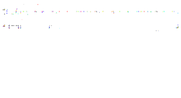
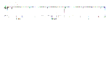
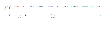
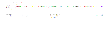
Figure 2: Time series data generated by Eqs. (5)–(8). Irregular fluctuations are observed in all variables with different time scales. The behaviour of $x_{1}$ is slow, that of $x_{2}$ is fast, and that of $x_{3}$ and $x_{4}$ is moderate.

To construct directed networks from the perspective of the underlying linear periodic structures we construct the network using summarized information of the models. The basic idea of the summarized information is as follows. We distinguish the species of the time series, $x_{i}$, from a value of the species at a specific time, $x_{i}(t-l)$, by the term, “component” $x_{i}$. For $x_{i}(t-l)$, in contrast, we use the term, “variable”. We treat the components as the nodes of the network.

We first consider System 1, Eqs. (1)–(4). Eq. (1) shows that the component $x_{1}$ is influenced by three components, $x_{1}$, $x_{2}$ and $x_{4}$. That is, $x_{1}$ should be connected to $x_{2}$ and $x_{4}$. Similarly, since Eq. (2) shows that $x_{2}$ is driven only by itself, $x_{2}$ has no connection. Since Eq. (3) shows that $x_{3}$ is driven by $x_{1}$ and $x_{4}$, $x_{3}$ should be connected to $x_{1}$ and $x_{4}$. Finally, since Eq. (4) shows that $x_{4}$ is driven by $x_{1}$ and $x_{4}$, $x_{4}$ should be connected to $x_{1}$. The whole relationship in terms of connectivity is represented by the following set of reduced expressions:

$$x_{1} =f_{1}(x_{2},x_{4}),$$ (9)

$$x_{2} =0,$$ (10)

$$x_{3} =f_{3}(x_{1},x_{4}),$$ (11)

$$x_{4} =f_{4}(x_{1}),$$ (12)

where $f_{i}$ stands for the function representing connectivity of the $i$-th component $x_{i}$ and zero means that there is no connection. These expressions indicate the essential linear periodic structures and can be treated as summary information.

The summarized information of System 2 using this idea, Eqs. (5)–(8), is

$$x_{1} =f_{1}(x_{2}),$$ (13)

$$x_{2} =0,$$ (14)

$$x_{3} =f_{3}(x_{2}),$$ (15)

$$x_{4} =f_{4}(x_{2}).$$ (16)

The directed networks constructed based on these summary information are shown in Fig. 3. As the summarized information reflects the underlying linear periodic structures of the system, we consider that the networks are not peculiar but reasonable and natural. Hence, when we obtain multivariate time series we like to construct networks provided with these properties.

There is one point to be mentioned. One may think that the time delay information is lost in the network, as the delays themselves are not encoded in the links. However, this is not necessarily true in our opinion. The connections reflect some (possibly unknown) time delays, and the time delay connectivity structure is still indirectly encoded in the network, but the strength and particular value of time delays are not retained indeed.

As shown in Fig. 1, the behaviours of System 1 generated by Eqs. (1)–(4) show irregular fluctuations and it is difficult to know the relationship among the data by visual inspection. On the other hand, as shown in Fig. 2, the behaviours of $x_{3}$ and $x_{4}$ in System 2 seem to be very similar. However, this similarity is deceptive. As Eqs. (15) and (16) indicate, although both of $x_{3}$ and $x_{4}$ are influenced by $x_{2}$, $x_{4}$ is not included in the function of $x_{3}$, and $x_{3}$ is not included in the function of $x_{4}$. That is, there is no direct connection to between $x_{3}$ and $x_{4}$.

In the next section we describe fundamental problems with the current approaches and show that the current approaches fail to construct the networks shown Fig. 3.

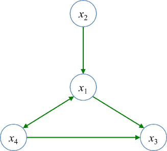
(a)   (b)

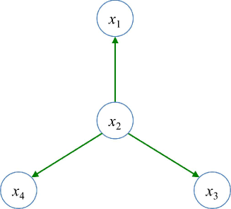
Figure 3: (Colour online) The network and the directed connectivity: (a) the first system, Eqs. (9)–(12), and (b) the second system, Eqs. (13)–(16).

4 Fundamental problems with the current approaches

The directed transfer function (DTF) and the partial directed coherence (PDC) are widely accepted methods as the frequency-based approach, and the naive method utilizing the cross correlation (CC) function is extensively used method of time-based approach.

In the first place, we discuss about using the multivariate auto-regressive (MVAR) model. Both DTF and PDC are based on the detection of phase differences between two signals. The reliability of the detection obviously depends on the quality of the MVAR model. However, MVAR model cannot meet the expectation. When building a MVAR model the conventional strategy is to increase the time delay of all variables progressively [15]. The optimal model is the one that has the smallest value of a chosen information criterion among many models [26]. In this strategy, a new term is always added to the previous model at each step, irrespective of whether the new term is indeed necessary or not. Furthermore, a set of multivariate time series might simultaneously include both short term (high frequency) and long term (low frequency) effects. To treat such multivariate time series appropriately, the model must include terms with delays of separated time scales corresponding to each effect. This is the so-called embedding problem [16]. This means that MVAR model often does not contain necessary terms which reflect peculiarities of time series.

The fact that all variables with the same time delays are included in MVAR models, irrespective of whether some of them are necessary or not, can cause a problem in parameter estimation, especially when there is strong collinearity among terms. In this case, some parameters have very large or small values [27]. The value of DTF and PDC is obtained using the coefficient of MVAR models [2, 3, 4, 7]. Using unreliable coefficients might cause a serious problem. One of the main purposes to adopt statistical modeling technique is to extract the underlying nature of the data. However, the MVAR model is obviously inappropriate in this respect. Since DTF and PDC are based on MVAR modeling, the results obtained by these methods might be unreliable in some cases.

Next, we discuss about using cross correlation (CC). To determine whether two nodes should be connected, the CC function is used in the naive method. In this approach it is basically expected that there are some sort of direct influence between two signals when these are similar. Then, it is considered that “similarity” is equivalent to “relationship” and “no similarity” is equivalent to “no relationship.” This idea does not always work well [25]. The CC function is only a useful measure of linear similarity. More precisely, the CC function is inherently a useful statistic to examine a rectilinear proportional relationship between two signals. However, even if the superposition principle is assumed, a rectilinear proportional relationship among some data is not always retained. As experimental time series will typically show some irregular fluctuations, the CC function will often be insufficient.

Finally, the frequency-based and the time-based approaches both need a threshold value to determine the existence of relationship. It is difficult to select an appropriate threshold and to determine the precise relationship among the various variables by a threshold value.

We explicitly show that all of DTF, PDC and the naive method fail for two systems with linear periodic structures, Eqs. (1)–(4) and Eqs. (5)–(8), which we introduced in Section 3.

4.1 Failure of the current approaches

Eqs. (1)–(4) of System 1 generate time series with similar time scales and Eqs. (5)–(8) of System 2 generate time series with different time scales. We use 1000 data points and the data are contaminated by Gaussian observational noise with the mean zero and the standard deviation 0.01. We apply DTF, PDC and the naive method to the data generated by both systems and examine the existence of relationships according to usual procedures described in Section 2.3.

To apply DTF and PDC an appropriate MVAR model is necessary. Such a MVAR model is usually determined by Akaike Information Criterion (AIC) or Schwarz Information Criterion (SIC) [21]. The SIC formula is defined by

$$\mathrm{SIC}(k)=n\ln\frac{{\bf e}^{T}{\bf e}}{n}+k\ln n,$$ (17)

where $n$ is the number of data points, $k$ is the model size, and $\bf e$ is the fitting errors [29]. The best model selected by such an information criterion is treated as the appropriate MVAR model. In this paper we use SIC to find appropriate MVAR models.

4.1.1 System 1: the case of similar time scales

We first use data generated by Eqs. (1)–(4). When DTF and PDC are applied to the data, the size of the best MVAR model is three. As Eqs. (1)–(4) show, the largest time delays for $x_{1}$, $x_{2}$, $x_{3}$ and $x_{4}$ are $3$, $6$, $0$ and $9$, respectively. Hence, this indicates that the best MVAR model does not cover the time delays of $x_{2}$ and $x_{4}$. The summarized information obtained by DTF and PDC is $x_{1}=f_{1}(x_{2},x_{4})$, $x_{2}=0$, $x_{3}=f_{3}(x_{1})$ and $x_{4}=f_{4}(x_{1})$. Table 1 shows all the values of the CC function and all the values are smaller than the threshold value $0.5$. Based on the results we construct the networks. Figure 4 shows that the networks constructed by DTF, PDC and the naive method are different from network shown in Fig. 3(a). Fig. 4(a) shows the network constructed by DTF and PDC. Although there is no link between $x_{3}$ and $x_{4}$, other directed links are the same as that shown in Fig. 3(a). However, Fig. 4(b) shows that there is no link among the nodes in the network constructed by the naive method.

Table 1: The largest absolute values of the CC function of all possible pairs between the time lag $-10$ and $10$, where the number in the parentheses is the time lag when the CC function has the largest absolute value. The data are generated by Eqs. (1)–(4), and the values are estimated using 1000 data points.

	$x_{1}$	$x_{2}$	$x_{3}$	$x_{4}$
$x_{1}$	1.0000	—	—	—
$x_{2}$	0.4109 (-4)	1.0000	—	—
$x_{3}$	0.3293 (2)	0.0782 (5)	1.0000	—
$x_{4}$	0.3221 (2)	0.1240 (6)	0.3919 (-9)	1.0000

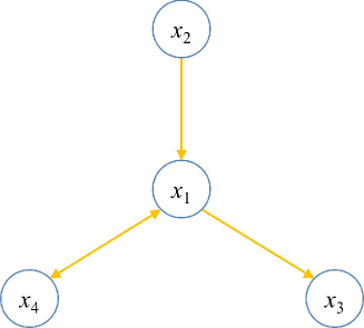
(a)   (b)

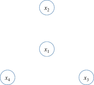
Figure 4: (Colour online) The linkage of constructed network using 1000 data points generated by generated by Eqs. (1)–(4). (a) the network when DTF and PDC are applied to the data, and (b) the network constructed by the naive method using the CC with the threshold $0.5$, The values of the CC are shown in Table 1. The network constructed by DTF and PDC are the same.

4.1.2 System 2: the case of distinct time scales

We next use data generated by Eqs. (5)–(8). When DTF and PDC are applied to the data, the size of the best MVAR model is four. As Eqs. (5)–(8) show, the largest time delays for $x_{1}$, $x_{2}$, $x_{3}$ and $x_{4}$ are $4$, $10$, $1$ and $1$, respectively. Hence, this indicates that the best MVAR model does not cover the time delay of $x_{2}$. The summarized information obtained by DTF is $x_{1}=f_{1}(x_{3})$, $x_{2}=f_{2}(x_{4})$, $x_{3}=f_{3}(x_{1},x_{2},x_{4})$ and $x_{4}=f_{4}(x_{2})$, and that obtained by PDC is $x_{1}=f_{1}(x_{2})$, $x_{2}=f_{2}(x_{4})$, $x_{3}=f_{3}(x_{2})$ and $x_{4}=f_{4}(x_{2})$.

Table 2 shows all the values of the CC function. Based on the results we construct the networks. Figure 5 shows that the networks constructed by DTF, PDC and the naive method are different from the network shown in Fig. 3(b). Figure 5(a) shows that DTF fails to detect the relationship between $x_{1}$ and $x_{2}$ and creates non-existent links between $x_{1}$ and $x_{3}$ and between $x_{3}$ and $x_{4}$. Figure 5(b) shows that connectivity in the network constructed by PDC is the same as that in Fig. 3(b). However, there is one non-existent directed link from $x_{4}$ and $x_{2}$. Figure 5(c) shows that the naive method fails to detect most of links and creates one non-existent link between $x_{3}$ and $x_{4}$. The value between $x_{3}$ and $x_{4}$ is larger than the commonly used threshold value $0.5$ [9, 10]. The behaviour of $x_{3}$ is visually similar to that of $x_{4}$ as shown in Fig. 2. Hence, it seems likely that there is direct relationship between them. However, it is clearly untrue.

Table 2: The largest absolute values of the CC function of all possible pairs between the time lag $-10$ and $10$, where the number in the parentheses is the time lag when the CC function has the largest absolute value. The data are generated by Eqs. (5)–(8), and the values are estimated using 1000 data points.

	$x_{1}$	$x_{2}$	$x_{3}$	$x_{4}$
$x_{1}$	1.0000	—	—	—
$x_{2}$	0.0903 (-10)	1.0000	—	—
$x_{3}$	0.1497 (10)	0.4693 (5)	1.0000	—
$x_{4}$	0.2322 (-10)	0.4969 (4)	0.7729 (-1)	1.0000

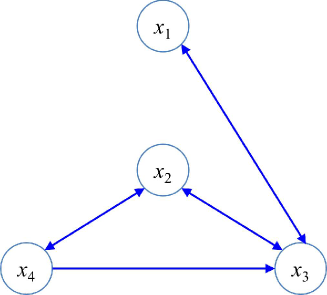
(a)   (b)
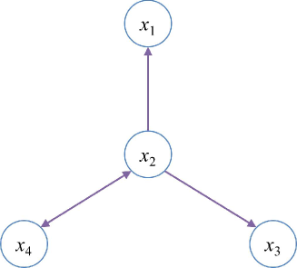
(c)

Figure 5: (Colour online) The linkage of constructed network using 1000 data points generated by generated by Eqs. (5)–(8). (a) the network when DTF is applied to the data, (b) the network when PDC is applied to the data, and (b) the network constructed by the naive method using the CC with the threshold $0.5$, The values of the CC are shown in Table 2.

4.1.3 Results of the current approaches

As mentioned in Section 4 MVAR model cannot always include terms with delays of separated time scales. In Sections 4.1.1 and 4.1.2 we found that the best MVAR models for both cases do not cover the largest time delay of some components. We are afraid of that this problem may happen at any moment. Even if the MVAR models do not contain necessary terms, it is acceptable if the constructed networks based on the MVAR models are the same as desired networks. However, the current approaches unfortunately cannot construct desired networks for the two examples.

We consider that there are at least four types of relationships for the elements of the assumed system: (i) unilateral influence from an element $A$ to an element $B$, (ii) unilateral influence from $B$ to $A$, (iii) mutual influence between $A$ and $B$, and (iv) influence to $A$ and $B$ from an independent (third-party) element $C$. It is preferable to be able to distinguish these relationships. In this respect, Zalesky et al. have pointed out that the CC function should be used cautiously in network construction [31]. In our opinion, this point has been overlooked by the user of the naive method.

Hence, the following four points are particularly important in constructing networks for multivariate time series: (1) multivariate time series may include both short time and long time effects, whose time scales are well separated, (2) we should be able to identify linear periodic structures included in multivariate data, (3) we should not be deceived by apparent behaviours of data, and (4) relationships among data should not be determined by an externally selected value of the threshold. Although these points are mentioned separately, these are strongly interconnected when constructing networks from multivariate time series. Furthermore, it will be preferable to construct directed networks. To fulfil these requirements and overcome the drawbacks with the current approaches we propose a method based on an information theoretic reduction of a linear (auto-regressive) model for multivariate time series.

5 An approach based on the reduced auto-regressive model

As indicated in Section 3, if we have enough information about the exact dynamical equations of the system, the faithful network representation can be obtained from the summarized information. Unfortunately, it is usually difficult to obtain the information in practice. In most cases, we have to start only from observed data without the knowledge of the underlying dynamical system. Hence, the main issue is to obtain the dynamical relationship among components as faithful as possible only from the observed multivariate time series data. We first consider this problem in cases where a perfect linear model of a system exists. We use Systems 1 and 2 introduced in Section 3, where the current approaches do not work well. In Section 6 we will consider this problem in uncertain situations, when no correct linear system of a system exists.

5.1 Reduced auto-regressive (RAR) model

To precisely identify the underlying linear periodic structures for multivariate time series we apply an information theoretic reduction of linear models, the reduced auto-regressive (RAR) model [15, 16]. There are strong information theoretic arguments to support that RAR model can detect any periodicities built into a given time series [17]. The RAR model includes terms only when their combination contributes significantly to the model as an entire system in terms of a suitably chosen information criterion [16] and allows to contain terms with short and large time delays concurrently unlike the AR model, even when the time scales of the delays are completely different. The RAR model is basically composed of the terms with time intervals (periodicities) at which underlying or characteristic situations (behaviours) are sharply or clearly repeated in the data, irrespective of whether the patterns or data are linear or nonlinear . The RAR model is thus effective in modelling both linear and nonlinear data [15, 16, 17]. We explicitly show in A that the RAR model can identify periodicities in both linear and nonlinear data.

An RAR model from given a univariate (scalar) time series is constructed as follows. Given a univariate time series $\{x(t)\}_{t=1}^{n}$ of $n$ observations, an RAR model with the largest time delay $l_{w}$ is expressed as

$$x(t) =a_{0}+a_{1}x(t-l_{1})+a_{2}x(t-l_{2})+\dots+a_{w}x(t-l_{w})+\varepsilon(t)$$

$$=a_{0}+\sum_{i=1}^{w}a_{i}x(t-l_{i})+\varepsilon(t),$$ (18)

where $1\leq l_{1}<l_{2}\cdots<l_{w}$, $a_{i}\;(i=0,1,2\dots,w)$ are parameters to be determined, and $\varepsilon(t)$ is assumed to be independent and identically distributed Gaussian random variables, which are interpreted as fitting errors. The parameters $a_{i}$ are chosen to minimize the sum of the squares of fitting errors. To build an RAR model we prepare candidate basis functions used in the modelling, in the form of a dictionary, and select the most appropriate basis functions that can extract the temporal structure of the time series. The number of candidate basis functions included in a dictionary is not restricted a priori. When we assume a linear model the basis functions are a constant and linear terms. For selecting basis functions, various algorithms have been proposed, which are proven to be effective in modelling both linear and nonlinear dynamics. The models obtained by these algorithms are considered to be nearly optimal [15, 16, 17, 32, 33]. In this paper, we adopt a selection algorithm using the total error [32], which will be described later in this subsection.

It is straightforward to apply this methodology to multivariate time series. A set of multivariate RAR models is expressed by

$$x_{i}(t)=a_{i,0}+\sum_{j=1}^{N}\left(\sum_{k=1}^{w_{j}}a_{i,j,k}\;x_{j}(t-l_{k})\right)+\varepsilon_{i}(t)\;\;\;(i=1,2,\dots,N),$$ (19)

where $N$ is the number of components and $l_{w_{i}}(\geq 0)$ is the largest time delay of the $i$-th component.

5.2 How to find an optimal RAR model

In what follows, an information criterion approach is used to evaluate and obtain the best (optimal) model among many. The model that gives the minimum of the information criterion is considered to be the best model [34, 35]. Various information criteria have been proposed for their own purposes [15, 29, 34, 36, 37]. For determining the best model we adopt the Description Length (DL) suitably modified by Judd and Mees [15], because the DL modified by Judd and Mees has proven to be effective in modelling nonlinear dynamics [16, 17], and it has fewer approximations than other information criteria, though slightly more calculations are needed [15]. Hence, the DL is more reliable for the present purpose [28].

When the $\varepsilon(t)$ and $\varepsilon_{i}(t)$ in Eqs. (18) and (19) are assumed to be Gaussian and the $a_{i}$ and $a_{i,j,k}$ in Eqs. (18) and (19) have been chosen to minimise the sum of squares of the prediction errors ${\bf e}=y-\hat{y}$ where $y$ is the observational data and $\hat{y}$ is the predicted data, Judd and Mees show that the description length is bounded by

$$DL(k)=\left(\frac{n}{2}-1\right)\ln\frac{{\bf e}^{T}{\bf e}}{n}+\left(k+1\right)\left(\frac{1}{2}+\ln\gamma\right)-\sum_{i=1}^{k}\ln\delta_{i},$$ (20)

where $n$ is the length of the time series to be fitted, $k$ is the number of parameters (or model size), $\gamma$ is related to the scale of the data, and the variables $\delta$ can be interpreted as the relative precision to which the parameters are specified. The factor $\gamma$ is a constant and typically fixed to be $\gamma=32$ [15]. The first term in the description length equation, $\left(\frac{n}{2}-1\right)\ln\frac{{\bf e}^{T}{\bf e}}{n}$, is the penalty for the model prediction errors and is derived from the conventional log-likelihood expression. In the case of DL that derivation is a little circuitous as the DL penalty is measuring the cost of encoding those errors. More thorough arguments for the details of the RAR model and the DL can be found in [15, 16].

To build an RAR model we need to select the optimal subset from a dictionary of basis functions. In this paper, we use a selection algorithm using the total error, because this algorithm is able to obtain better models in most cases than others with reasonable computation time [32]. As the bottom-up approach has proven to be effective [15, 16, 17], we first apply the bottom-up method using the total error [32]. In searching for the best model, we might be trapped in one of the local minima of the Description Length. To avoid this situation and to reduce the problem to a manageable size, a model is also built from the complete dictionary using the top-down method, but starting from the model whose size is 10 larger than that of the best model obtained by the bottom-up method. This method do no worse than the bottom-up method. For more details on this procedure and the relevant approaches see [15, 16, 17, 32, 38]. We select the model as the best model whose description length is the smallest with this procedure. However, it should be noted that selecting the optimal subset from a dictionary is an NP-hard problem that usually has to be solved heuristically [15]. We will discuss more on the problems or difficulties with building RAR models in Section 7.

5.3 Confirmation of reproducibility

We apply the RAR modelling technique to the data represented in Figs. 1 and 2 to investigate whether we can reconstruct System 1, Eqs. (1)–(4), and System 2, Eqs. (5)–(8), only from the generated data sets. In this case, we have four time series (that is, $x_{1}(t)$, $x_{2}(t)$, $x_{3}(t)$ and $x_{4}(t)$) of 1000 data points with Gaussian observational noise for each data set. For Gaussian observational noise, we use four different noise level with the standard deviation 0.01, 0.02, 0.05 and 0.1. All of the mean values are fixed to zero. For each observational noise level, we prepare five sets of time series with different noise realizations. Choosing time delays up to 10 for time series of each component and the constant function give 41 candidate basis functions in the dictionary. Using the dictionary we build the multivariate RAR model for four components, $x_{1}$, $x_{2}$, $x_{3}$, and $x_{4}$. We show some of the results when the observational noise level is 0.01. The best models for System 1, Eqs. (1)–(4), are

$$x_{1}(t) =1.1547+0.4123\;x_{1}(t-1)-0.2185\;x_{1}(t-3)$$

$$\phantom{=}+0.3148\;x_{2}(t-4)+0.2359\;x_{4}(t-7),$$ (21)

$$x_{2}(t) =1.8172+0.6541\;x_{2}(t-1)-0.1952\;x_{2}(t-6),$$ (22)

$$x_{3}(t) =2.1602+0.2030\;x_{1}(t-2)+0.3102\;x_{4}(t-9),$$ (23)

$$x_{4}(t) =1.2227+0.2390\;x_{1}(t-2)+0.4879\;x_{4}(t-1)$$

$$\phantom{=}-0.3013\;x_{4}(t-3),$$ (24)

and the best models for System 2, Eqs. (5)–(8), are

$$x_{1}(t) =12.1800+1.2967\;x_{1}(t-1)-0.3054\;x_{1}(t-4)+0.2217\;x_{2}(t-3),$$ (25)

$$x_{2}(t) =0.3227\;x_{2}(t-1)+0.1969\;x_{2}(t-6),$$ (26)

$$x_{3}(t) =1.1935\;x_{2}(t-4)-0.6524\;x_{2}(t-10)+0.9441\;x_{3}(t-1),$$ (27)

$$x_{4}(t) =5.6114\;x_{2}(t-3)+0.9193\;x_{4}(t-1).$$ (28)

Eqs. (21)–(24) and Eqs. (25)–(28) show that all terms included in Eqs. (1)–(4) and Eqs. (5)–(8) and only these terms are selected, which means that the same networks as those shown in Fig. 3 is constructed. When the RAR modelling technique is applied to the data in all of the other cases, the situations are the same: only all the terms included in Eqs. (1)–(4) and Eqs. (5)–(8) are selected. This reproducibility manifests the strong power of the proposed method for identifying necessary terms.

6 Imperfect model scenario: when no correct linear system of a system exists

Thus far we have restricted attention to the perfect model scenario. The cases we considered were that correct linear models exist and time series are generated by the linear systems including the time delay terms corresponding to the periodicities. That is, there are explicit linear periodic structures among multivariate time series. We confirmed that the RAR model procedure precisely identifies the linear periodic structures and then the correct networks are constructed. However, there may not always be the case, because even if time series exhibit periodicities (either exactly periodic and nearly periodic behaviour), the system may not contain terms corresponding to the periodicities. In such a case correct linear systems exist no more or steadfast linear models might not be possible to assume. Hence, it is important to not build the correct models but construct the correct network in this case. To investigate how the proposed method works in uncertain situations, we use the Rössler systems presented in the form of a differential equation as an example. The equations are given by

$$dx/dt = -y-z,$$ (29)

$$dy/dt = x+ay,$$ (30)

$$dz/dt = b+z(x-c),$$ (31)

where $a=0.398$, $b=2.0$, $c=4.0$ [39]. There is a nonlinear term $z\;x$ in Eq. (31) and the equations can exhibit chaotic behaviours when using these parameters [40]. We calculate the equations using the fourth order Runge-Kutta method with sampling interval 0.01. As Figs. 6(a)–(c) show, although time series of each variable is oscillating, Fig. 6(d) shows that the attractor is chaotic.

Broadly speaking, the meaning of a differential equation is that a change (or difference) of a variable in a minute time is expressed by a certain function. For example, Eq. (29) indicates that the next value (or state) of $x$ is calculated as the summation of the current value of $x$ and the minute current value of $-y-z$. That is, although the right side of Eq. (29) does not contain $x$, $x$ is a function composed of $x$, $y$ and $z$ in a practical sense. Hence, $y$ is a function of $x$ and $y$, and $z$ is a function of $x$ and $z$ in a similar way.

(a)

(b) (c)

(d)

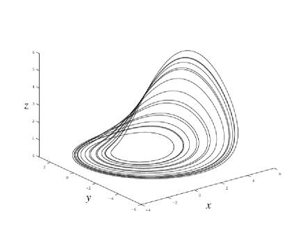
Figure 6: Time series and attractor generated by the Rössler systems, Eqs. (29)–(31), where the number of data points is 10 000. (a) $x$ component, (b) $y$ component, (c) $z$ component, and (d) attractor composed of $x$, $y$ and $z$. Although these time series look periodical behavious as shown in Figs. 6(a)–(c), Fig. 6(d) shows that these are chaotic behaviours in reality.

We first investigate the influence of the number of data points. We use four different data points, 1000, 2000, 5000 and 10 000 and prepare five sets of time series. These data are contaminated by Gaussian observational noise with the mean zero and the standard deviation 0.01. As there are three time series, choosing a time delay up to 20 for time series of each data and the constant function give 61 candidate basis functions in the dictionary. Using the dictionary we build the multivariate RAR model for each data, $x$, $y$ and $z$.

The summarized information of the obtained three multivariate RAR models are shown in Table 3. In all cases the information for $x$ and $y$ are correct. However, the information for $z$ is different. When the number of data points is 1000, the correct information for $z$ cannot be obtained at all. When the number of data points is 2000, although the correct information for $z$ is obtained, the wrong information is also obtained. When the numbers of data points is 5000 and 10 000, the correct information for $z$ is always obtained. We consider that as there is a nonlinear term $z\;x$ as shown in Eq. (31), the more data points are necessary for $z$ to extract the correct relationship among $x$, $y$ and $z$.

Table 3: Investigation of the influence of the number of data points. The components contained in the multivariate RAR models using data generated by the Rössler systems shown in Fig. 6. The numbers of data points are 1000, 2000, 5000 and 10 000, five sets of time series are used, and the data are contaminated by Gaussian observational noise with the mean zero and the standard deviation 0.01. The value in parentheses is the number of times the result occurred. As we use five sets for each data point, if the same result is always obtained, the value in parentheses is $5$.

	1000	2000	5000	10 000
$x$	$x~{}y~{}z~{}(5)$	$x~{}y~{}z~{}(5)$	$x~{}y~{}z~{}(5)$	$x~{}y~{}z~{}(5)$
$y$	$x~{}y~{}(5)$	$x~{}y~{}(5)$	$x~{}y~{}(5)$	$x~{}y~{}(5)$
$z$	$z~{}(4),~{}y~{}z~{}(1)$	$z~{}(2),~{}x~{}z~{}(3)$	$x~{}z~{}(5)$	$x~{}z~{}(5)$

We could confirm in the previous investigation that the correct relationships are obtained as the number of data points increases. We next investigate the influence of observational noise using four different noise levels. We use 10 000 data points and the data are contaminated by Gaussian observational noise with the mean zero and the standard deviation 0.01, 0.02, 0.05 and 0.1. We prepare five sets of time series for each noise level. Choosing a time delay up to 20 for time series of each data and the constant function give 61 candidate basis functions in the dictionary. Using the dictionary we build the multivariate RAR models. The summarized information are shown in Table 4. The information for $x$ are correct in all cases, and the correct information for $y$ and $z$ is obtained when the observational noise level is 0.01, 0.02 and 0.05. However, when the observational noise level is 0.1, although the correct information is obtained, the wrong information is also obtained. This indicates that there are cases that the correct information cannot be obtained when the observational noise level is large.

Table 4: Investigation of the influence of the observational noise. The components contained in the multivariate RAR models using data generated by the Rössler systems shown in Fig. 6. The number of data points is 10 000, five sets of time series are used, and the data are contaminated by Gaussian observational noise with the mean zero and the standard deviation 0.01, 0.02, 0.05 and 0.1. The value in parentheses is the number of times the result occurred.

	0.01	0.02	0.05	0.1
$x$	$x~{}y~{}z~{}(5)$	$x~{}y~{}z~{}(5)$	$x~{}y~{}z~{}(5)$	$x~{}y~{}z~{}(5)$
$y$	$x~{}y~{}(5)$	$x~{}y~{}(5)$	$x~{}y~{}(5)$	$x~{}y~{}(2),~{}x~{}y~{}z~{}(3)$
$z$	$x~{}z~{}(5)$	$x~{}z~{}(5)$	$x~{}z~{}(5)$	$x~{}z~{}(1),~{}y~{}z~{}(3),~{}x~{}y~{}z~{}(1)$

7 Reexamination of the proposed method

In building an RAR model, it is necessary to select terms with important time delays with an appropriate information criterion to find the optimal model. The obtained optimal model is thus influenced by the employed combination of the selection method and the information criterion.

A variety of information criteria, such as Akaike Information Criterion, Schwarz Information Criterion, Description Length, and so on, have already been proposed with their own different backgrounds [28]. It means that the optimal models corresponding to different information criteria are not necessarily identical, even if we compare all possible values of the criteria calculating all possible combinations of terms. As each best model reflects each background of the employed information criterion, we should be careful in comparing the results by taking these backgrounds into consideration.

Apart from the selection of information criterion, the calculation of possible combinations of terms causes another concern. The number of all combinations explodes as the number of components in the time series increases. Selecting the optimal subset from a dictionary of basis functions thus becomes an NP-hard problem and has to be solved heuristically [15]. Various heuristic algorithms have been proposed for selecting basis functions [15, 32, 41] and some optimization approaches can be applied for the modelling, for example, simulated annealing, genetic algorithm, deep learning and so on [42, 43, 44]. Also, another idea has been introduced to impose a sparseness constraint onto MVAR model [45]. An important point when we employ non-exhaustive search is that the selected model might be not optimal but nearly optimal corresponding to a local minimum of an employed information criterion [16]. Hence, we should take care in choosing a selection algorithm and should check the plausibility of the selected model. In this paper, we choose the Description Length modified by Judd and Mees for the information criterion [15, 16] and the selection method using total error for the heuristic algorithm [32]. The reason for this choice is simply because this combination of information criterion and selection method has been proven to be effective in modelling both linear and nonlinear dynamics and to obtain better models in many cases [32]. Although we understand that there are many other alternatives, exhaustive comparison between them would be far beyond the scope of this work. However, we note that an idea of using summarized information of the RAR model to construct the directed network is central to this approach.

The proposed method (and the current approaches alike) does not work well when there is no linear periodic structure in the data. One typical example is the Logistic map [46]. It is well known that the Logistic map is a nonlinear system that lacks clear periodicity, as the randomness is equivalent to that of IID random variables. The proposed method and the current approaches as well cannot treat such a data appropriately. We need an alternative approach to tackle it theoretically.

7.1 Connection to Granger causality

The proposed method constructs a directed network using components composed of multivariate RAR models. We consider that the Granger causality using MVAR models provides a similar statistical approach [47].

We consider that the Granger causality is useful, but also very restrictive because of the following two problems. Although these problems will be mentioned separately, they are strongly interconnected. One is to use MVAR models, and the other is to use prediction accuracy. As mentioned in Section 4, MVAR models have difficulties in treating peculiarities of data appropriately. Such a model often becomes unstable and also has difficulty in prediction. We need to treat the prediction accuracy carefully [15]. One of the strong reasons is that data available to us are usually contaminated by observational noise to a varying degree and the true dynamics in a phenomenon is intertwined with observational noise in time series. Hence, the high prediction accuracy means that the model provides similar behaviour to not that of the true phenomenon but that of the noisy data. That is, the model should not be fitted to the data too closely [15].

We consider that the true concept (or true intent) of the Granger causality principle is that the components are recognized to have causality, if the role and importance of the components for a model cannot be ignored. RAR models include only terms that contribute significantly to the model, as assessed by an information criterion. Although RAR models does not refer to the causal relationship, we consider that the proposed method adheres faithfully to the concept of the Granger causality in this sense.

8 Applications

Based on the thorough arguments and the results of these computational studies, we apply the proposed method to two experimental systems: (i) hourly meteorological time series in Kobe, Japan and (ii) multichannel electroencephalography time series with 10 channels (measured during resting state with eyes closed). As shown in Figs. 7 and 9, each of them exhibits irregular fluctuations.

The naive method remains the most commonly used approach, because of its conceptual and computational simplicity [5, 8, 12]. Hence, we also show the networks constructed by the naive method from the same data sets for comparison.

8.1 Meteorological data in Kobe, Japan

The meteorological data set consists of five time series: the atmospheric pressure, the atmospheric temperature, the dew-point temperature, the vapour pressure and the humidity, taken hourly in Kobe, Japan from 1 January to 12 February in 2013. The measurement location is 34^∘–41.8${}^{{}^{\prime\prime}}$ north latitude and 135^∘–12.7${}^{{}^{\prime\prime}}$ east longitude. From the profiles of the time series shown in Fig. 7, the relationship among these five time series is complicated and hard to be extracted.

(a)   (b)
(c)   (d)
(e)

Figure 7: Hourly meteorological time series in Kobe, Japan from 1 January to 12 February in 2013: (a) atmospheric pressure, (b) temperature, (c) dew-point temperature, (d) vapour pressure, and (e) humidity. These data are used for building multivariate RAR models.

We use 1000 data points (about 42 days) for building multivariate RAR models. As there are five time series, choosing a time delay up to 15 for time series of each data and the constant function give 76 candidate basis functions in the dictionary. Using the dictionary we build the multivariate RAR model for each data. The summarized information of the obtained five multivariate RAR models are

$$x_{1} =f_{1}(x_{2}),$$ (32)

$$x_{2} =f_{2}(x_{4}),$$ (33)

$$x_{3} =0,$$ (34)

$$x_{4} =f_{4}(x_{3}),$$ (35)

$$x_{5} =f_{5}(x_{2},x_{3}),$$ (36)

where $x_{1}$ corresponds to the atmospheric pressure, $x_{2}$ the atmospheric temperature, $x_{3}$ the dew-point temperature, $x_{4}$ the vapour pressure, $x_{5}$ the humidity, and zero means that there is no connection.

Figure 8(a) shows the directed network constructed by the proposed method. The numbers of in-degree and out-degree for each node in Fig. 8(a) are shown in Table 5. From these results we find that the atmospheric pressure and the humidity are influenced by others but do not have influence on any other components. On the contrary, the dew-point temperature is not influenced by others but has influence on the other two components. The atmospheric temperature and the vapour pressure are influenced by others and have influence on others at the same time. We also found that there is no mutual (bi-directional) connections among any component.

For comparison we show the network obtained by the naive method in Fig. 8(b), where the cross correlation (CC) function is evaluated between the time lag $-15$ and $15$ with the threshold $0.5$. Table 6 shows all the values. There are similarities and differences between Figs. 8(a) and 8(b). The link between $x_{1}$ and $x_{2}$ in Fig. 8(a) is absent in Fig. 8(b). The time dependencies of $x_{1}$ and $x_{2}$ in Figs. 7(a) and 7(b), are clearly dissimilar and the largest absolute value of the CC function is no more than $0.1779$. We consider that the RAR modelling technique uncovered a hidden relationship between these components. On the other hand, there are two links between $x_{2}$ and $x_{3}$ and between $x_{4}$ and $x_{5}$ in Fig. 8(b), which are absent in Fig. 8(a). We consider that these “redundant” links can be understood as “indirect” relationships deducible from the directed network in Fig. 8(a). For example, the link between $x_{2}$ and $x_{3}$ in Fig. 8(b) can be deduced from two consecutive directed links from $x_{3}$ to $x_{4}$ and from $x_{4}$ to $x_{2}$ in Fig. 8(a). The link between $x_{4}$ and $x_{5}$ in Fig. 8(b) can also be deduced from two consecutive directed links from $x_{4}$ to $x_{2}$ and from $x_{2}$ to $x_{5}$.

We consider the interactions between these five physical quantities. As the air becomes lighter (heavier) when the temperature becomes higher (lower), it is generally considered that the change of the temperature brings about the change of the atmospheric pressure. As there is a directed link from $x_{2}$ to $x_{1}$ on the network as shown in Fig. 8(a), where $x_{1}$ is atmospheric pressure and $x_{2}$ is temperature, we consider that the proposed method can correctly identify the relationship. However, Fig. 8(b) shows that there is no link between $x_{1}$ and $x_{2}$. Hence, this indicates that the naive method fails to detect this relationship. It is also known that there is no relationship between the temperature and the dew-point temperature. Although the proposed method shows that there is no relationship between the temperature and the dew-point temperature ($x_{2}$ and $x_{3}$), the naive method shows that there is relationship between them.

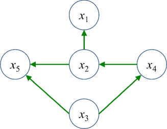
(a)   (b)

Figure 8: (Colour online) Networks of meteorological time series taken hourly in Kobe, Japan from 1 January to 12 February in 2013: (a) the directed network constructed by the proposed method, and (b) the network constructed by the naive method using the CC with the threshold $0.5$, where $x_{1}$ corresponds to atmospheric pressure, $x_{2}$ temperature, $x_{3}$ dew-point temperature, $x_{4}$ vapour pressure, and $x_{5}$ humidity.

Table 5: The number of in-degree and out-degree of the directed network of meteorological data shown in Fig. 8(a).

	atmospheric	temperature	dew-point	vapour	humidity
	pressure		temperature	pressure
in-degree	1	1	0	1	2
out-degree	0	2	2	1	0

Table 6: The largest absolute values of the CC function of all possible pairs between the time lag $-15$ and $15$, where the number in the parentheses is the time lag when the CC function has the largest absolute value. The data are hourly meteorological time series shown in Fig. 7. The values of the CC function are estimated using 1000 data points.

	$x_{1}$	$x_{2}$	$x_{3}$	$x_{4}$	$x_{5}$
$~{}~{}~{}~{}x_{1}~{}~{}~{}~{}$	1.0000	—	—	—	—
$x_{2}$	0.1779 (-3)	1.0000	—	—	—
$x_{3}$	0.2622 (-6)	0.6977 (-3)	1.0000	—	—
$x_{4}$	0.2996 (-4)	0.6951 (-2)	0.9778 (0)	1.0000	—
$x_{5}$	0.2667 (-8)	0.5634 (-11)	0.7341 (0)	0.7183 (0)	1.0000

We can explore the obtained network using the summarized information, Eqs. (32)–(36). We expect that this approach is effective for more complicated cases. We consider the case between $x_{2}$ and $x_{3}$ again. Eq. (33) is $x_{2}=f_{2}(x_{4})$ and Eq. (35) is $x_{4}=f_{4}(x_{3})$. As Eq. (33) shows that $x_{4}$ is included in $f_{2}$, we can rearrange Eq. (33) using Eq. (35). The rearrangement gives

$$x_{2} =f_{2}(x_{4}),$$ (37)

$$=f_{2}(f_{4}(x_{3})),$$ (38)

$$=f^{\prime}_{2}(x_{3}),$$ (39)

where $f^{\prime}_{2}$ is a new function for $x_{2}$. Eq. (39) explicitly shows the “indirect” relationship between $x_{2}$ and $x_{3}$.

8.2 Electroencephalogram (EEG) data

The second application is to EEG data. The EEG signal we use here was recorded from a healthy human adult during resting state with eyes closed in an electrically shielded room. The EEG data were simultaneously obtained from 10 channels of Fz, Cz, Pz, Oz, F3, F4, C3, C4, P3 and P4 of the unipolar 10-20 Jasper registration scheme [48]. Mono-polar recordings, referenced to linked earlobes, were obtained from these channels using an Electrocap. Vertical and horizontal eye movements were recorded, respectively, from electrode sites above and below the right eye and from near the outer canthi of each eye. Artefact corrupted records were removed from the analyses. The data were digitized at 1024 Hz using a twelve-bit digitizer. The EEG impedances were less than 5[K$\Omega$]. The data were amplified by gain = 18 000, and amplifier frequency cut-off settings of 0.03 Hz and 200 Hz were used [49]. We use 1000 data points (around 1 second) to build multivariate RAR models. Figure 9 shows time series of each channel.

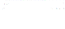
Figure 9: Multichannel electroencephalography (EEG) time series of Fz, Cz, Pz, Oz, F3, F4, C3, C4, P3 and P4 used for building multivariate RAR models.

As there are 10 channels, choosing a time delay up to 25 for time series of each channel and the constant function give 251 candidate basis functions in the dictionary. Using the dictionary we build the multivariate RAR model for each channel. The summarized information of the obtained 10 multivariate RAR models are

$$Fz =f_{Fz}(Cz),$$ (40)

$$Cz =f_{Cz}(Pz,Oz,F3),$$ (41)

$$Pz =f_{Pz}(Fz,Cz,Oz,C3,P3,P4),$$ (42)

$$Oz =f_{Oz}(Fz,Cz),$$ (43)

$$F3 =0,$$ (44)

$$F4 =f_{F4}(Fz),$$ (45)

$$C3 =f_{C3}(F3,P3),$$ (46)

$$C4 =f_{C4}(Fz,P4),$$ (47)

$$P3 =f_{P3}(Pz,Oz),$$ (48)

$$P4 =f_{P4}(Fz,Cz,Pz),$$ (49)

where zero means that there is no connection.

Figure 10 shows the network obtained by the proposed method and the one obtained by the naive method. In Fig. 10(a) obtained by the proposed method, the channels, Cz, Pz, P3, P4, and Oz, are mutually connected by bi-directional arrows. Figure 10(b) shows that the network obtained by the naive method has clearly more links than that by the proposed method. This result might indicate that the constructed network by the naive method has redundant links.

(a)   (b)

Figure 10: (Colour online) Network of EEG data shown in Fig. 9: (a) the directed network constructed by the proposed method, and (b) the network constructed by the naive method using the CC with the threshold $0.5$.

Table 7: The numbers of in-degree and out-degree for each node of the directed network of EEG data shown in Fig. 10(a).

	Fz	Cz	Pz	Oz	F3	F4	C3	C4	P3	P4
in-degree	1	3	6	2	0	1	2	2	2	3
out-degree	5	4	3	3	2	0	1	0	2	2

The numbers of in-degree and out-degree for each node in Fig. 10(a) are shown in Table 7. Table 7 shows that the node Pz has the largest in-degree and the node Fz has the largest out-degree. The largest in-degree of node Pz implies that the dynamics of the parietal areas captured by node Pz is under the influences of many other brain areas distributed over parietal and occipital parts of the brain. Since the parietal association areas are considered to be the parts that integrates sensory information from widely distributed parts of the brain, this result seems plausible. On the other hand, the largest out-degree of node Fz implies that the frontal areas recorded with node Fz has the influence over a wide-range of the brain. This is natural as the frontal brain areas are regarded to be involved in cognitive control and project top-down connections to lower brain areas.

We finally consider effects of the surface Laplacian briefly. Functional connectivity estimation with the proposed method may be contaminated by volume conduction effects [50]. Such effect would be relatively small for the current result as the RAR models utilizes terms with time delays, not just zero-lag correlations, to estimates the connections between nodes, although the RAR based on scalp EEG may not be free of the volume conduction as pointed out for DTF [51, 52, 53]. Also, the number of electrodes used in this study is just 10, implying that the volume conduction effect was small. For high density EEG where the volume conduction effect is more serious, the methods such as surface Laplacian [50] or source localization techniques would be useful [54]. Further studies would be necessary to investigate the effects of the volume conduction on the RAR based methods for functional connectivity estimation in a sensor space.

9 Summary

We have described an algorithm from constructing directed networks from multivariate time series based on the RAR model from the perspective of linear periodic structures (relationships). We also described the theoretical problems with the current approaches. We showed that the proposed method can extract reliable linear periodic structures among time series and that the constructed networks are considered to be faithful representation of the dynamical relationships. Our arguments and computational results show that the proposed method rectifies the drawbacks contained in the current approaches and constructs networks from multivariate time series faithfully.

We note that there are restrictions when applying the proposed method. RAR model cannot always identify nonlinear periodic structure in the data, and RAR model built using selection algorithms might not be the optimal. Hence, the network constructed by the proposed method might be near-optimal network in some cases. Moreover, it is difficult to build appropriate RAR models when the observational noise is large. Despite of these concerns, we believe that our method and the constructed networks has a wide range of applicability to real-world phenomena and provide us with useful information by using with care.

10 Acknowledgement

The authors thank to the anonymous referees for various valuable comments and suggestions. T.T. would like to acknowledge the support of a Grant-in-Aid for Scientific Research (C) (No. 24540419) from the Japan Society for the Promotion of Science (JSPS). M.S. is funded by Discovery Project (DP140100203). T.N. and the other authors would like to acknowledge Professor Paul E. Rapp (Uniformed Services University of the Health Sciences) for providing us with the EEG data used in Ref [49].

Appendix A Detecting periodicities from linear and nonlinear data using RAR model

We show that RAR model can identify periodicities in data, irrespective of whether the data is linear or nonlinear. We use the following system to generate linear data:

$$x(t)=a_{0}+a_{1}\;x(t-1)+a_{6}\;x(t-6)+\eta(t),$$ (50)

where $a_{0}=2.945~{}206$, $a_{1}=0.300~{}739$, $a_{6}=0.202~{}056$, and $\eta(t)$ is dynamic noise, IID Gaussian random variables with mean zero and standard deviation 1.0 [17]. The behaviour of the time series is shown in Fig. 11(a).

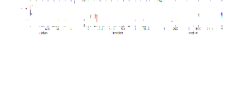
(a)   (b)
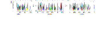
(c)   (d)

Figure 11: The behaviours of linear and nonlinear data and plots of description length $DL$ against size of model using the bottom-up method using the total error. We use these data to build RAR models to identify periodicities in the data. (a) linear data from Eq. (50), (b) nonlinear data transformed by a nonlinear function, Eq. (51), (c) description length and model size of linear data shown in Fig. 11(a), and (d) description length and model size of linear data shown in Fig. 11(b),

For periodicity detection in nonlinear data, we distort the data generated by Eq. (50) by a static monotonic nonlinear function $h(x)$,

$$h(x)=\frac{\left[\frac{x-x_{min}-0.0001}{x_{max}-x+0.0001}\right]^{\rho}}{1+\left[\frac{x-x_{min}-0.0001}{x_{max}-x+0.0001}\right]^{\rho}},$$ (51)

where $x_{min}$ and $x_{max}$ are the minimum and maximum value of $x(t)$ in the original time series, and $\rho=3$ [55]. The behaviour of the time series is shown in Fig. 11(b). It should be noticed that the nonlinear data have the same periodicities as those of the linear data, even though the nonlinear data are heavily distorted by a nonlinear function.

As the observational data, we use the 1000 data points with Gaussian observational noise with the mean zero and the standard deviation 0.01 for linear data and 0.003 for nonlinear data, respectively. These noise levels are equivalent to $1\%$ to both the data. Choosing a time delay=10 gives 11 candidate basis functions in the dictionary. These are the constant function and the linear terms, $x(1-1),x(t-2),\dots,x(t-10)$. We apply the bottom-up method using the total error and the exhaustive search both to the dictionary of the linear data and that of the nonlinear data. As shown in Figs. 11(c) and 11(d), the description length is the smallest when the model size is $3$ in both the linear and the nonlinear cases. In both cases, only the terms included in Eq. (50) (a constant, $x(t-1)$, and $x(t-6)$) are selected. That is, the correct model is selected as the best model. The exhaustive search also selects the correct model as the best model. This result indicates that the RAR model is effective in identifying periodicities for linear and nonlinear data.

References

- [1] T. Ohira, T. Yamane, Delayed stochastic systems, Physical Review E 61 (2000) 1247–1257.
- [2] M. J. Kamiński, K. J. Blinowska, A new method of the description of the information flow in brain structures, Biological Cybernetics 65 (1991) 203–210.
- [3] M. Kamiński, M. Ding, W. A. Truccolo, S. L. Bressler, Evaluating causal relations in neural systems: granger causality, directed transfer function and statistical assessment of significance, Biological Cybernetics 85 (2001) 145–157.
- [4] L. A. Baccalá, K. Sameshima, Partial directed coherence: a new concept in neural structure determination, Biological Cybernetics 84 (2001) 463–474.
- [5] R. N. Mantegna, Hierarchical structure in financial markets, The European Physical Journal B 11 (1) (1999) 193–197.
- [6] I. Farkas, H. Jeong, T. Vicsek, A.-L. Barabási, Z. N. Oltvai, The topology of the transcription regulatory network in the yeast, saccharomyces cerevisiae, Physica A 318 (3–4) (2003) 601–612.
- [7] L. Astolfi, F. Cincotti, D. Mattia, M. G. Marciani, L. A. Baccala, F. de Vico Fallani, S. Salinari, M. Ursino, M. Zavaglia, L. Ding, J. C. Edgar, G. A. Miller, B. He, F. Babiloni, Comparison of different cortical connectivity estimators for high-resolution eeg recordings, Human brain mapping 28 (2) (2007) 143–157.
- [8] K. Yamasaki, A. Gozolchiani, S. Havlin, Climate networks around the globe are significantly affected by el niño, Physical Review Letters 100 (22) (2008) 228501.
- [9] A. Tsonis, K. Swanson, Topology and predictability of el niño and la niña networks, Physical Review Letters 100 (22) (2008) 228502.
- [10] C. K. Tse, J. Liu, F. C. M. Lau, A network perspective of the stock market, Journal of Empirical Finance 17 (4) (2010) 659–667.
- [11] Z. Gao, N. Jin, Complex network from time series based on phase space reconstruction, Chaos 19 033137.
- [12] M. Nagy, Z. Ákos, D. Biro, T. Vicsek, Hierarchical group dynamics in pigeon flocks, Nature (London) 464 (2010) 890–894.
- [13] K. Iwayama, Y. Hirata, K. Takahashi, K. Watanabe, K. Aihara, H. Suzuki, Characterizing global evolutions of complex systems via intermediate network representations, Scientific Reports 2 (2012) 423.
- [14] Z.-K. Gao, M. Small, J. K. Kurths, Complex network analysis of time series, Europhysics Letters 116 (5) (2016) 50001.
- [15] K. Judd, A. Mees, On selecting models for nonlinear time series, Physica D 82 (1995) 426–444.
- [16] K. Judd, A. Mees, Embedding as a modeling problem, Physica D 120 (1998) 273–286.
- [17] M. Small, K. Judd, Detecting periodicity in experimental data using linear modeling techniques, Physical Review E 59 (1999) 1379–1385.
- [18] K. J. Blinowska, Review of the methods of determination of directed connectivity from multichannel data, Medical & Biological Engineering & Computing 49 (2011) 521–529.
- [19] K. Sameshima, L. A. Baccalá (Eds.), Methods in Brain Connectivity Inference through Multivariate Time Series Analysis (Frontiers in Neuroengineering Series), CRC Press, Boca Raton, 2014.
- [20] M. Kamiński, M. Ding, W. A. Truccolo, S. L. Bressler, Evaluating causal relations in neural systems: granger causality, directed transfer function and statistical assessment of significance., Biological Cybernetics 85 (2001) 145–157.
- [21] J. Toppi, F. D. V. Fallani, G. Vecchiato, A. G. Maglione, F. Cincotti, D. Mattia, S. Salinari, F. Babiloni, L. Astolfi, How the statistical validation of functional connectivity patterns can prevent erroneous definition of small-world properties of a brain connectivity network, Computational and Mathematical Methods in Medicine 2012 (2012) 130985.
- [22] J. Theiler, S. Eubank, A. Longtin, B. Galdrikian, J. D. Farmer, Testing for nonlinearity in time series: the method of surrogate data, Physica D 58 (1992) 77–84.
- [23] A. Galka, Topics in Nonlinear Time Series Analysis, World Scientific Publishing Company, Singapore, 2000.
- [24] M. Small, Applied Nonlinear Time Series Analysis, World Scientific Publishing Company, Singapore, 2005.
- [25] T. Nakamura, T. Tanizawa, M. Small, Constructing networks from a dynamical system perspective for multivariate nonlinear time series, Physical Review E 93 (2016) 032323.
- [26] G. Kitagawa, H. Akaike, A procedure for the modeling of non-stationary time series, Annals of the Institute of Statistical Mathematics 30 (1978) 351–363.
- [27] T. Nakamura, K. Judd, A. Mees, Refinements to model selection for nonlinear time series, International Journal of Bifurcation and Chaos 13 (5) (2003) 1263–1274.
- [28] T. Nakamura, K. Judd, A. I. Mees, M. Small, A comparative study of information criteria for model selection, International Journal of Bifurcation and Chaos 16 (8) (2006) 2153–2175.
- [29] G. Schwarz, Estimating the dimension of a model, Annals of Statistics 6 (1978) 461–464.
- [30] J. Theiler, D. Prichard, Constrained-realization monte-carlo method for hypothesis testing, Physica D 94 (1996) 221–235.
- [31] A. Zalesky, A. Fornito, E. Bullmore, On the use of correlation as a measure of network connectivity, NeuroImage 60 (2012) 2096–2106.
- [32] T. Nakamura, D. Kilminster, K. Judd, A. Mees, A comparative study of model selection methods, International Journal of Bifurcation and Chaos 14 (3) (2004) 1129–1146.
- [33] T. Nakamura, M. Small, Nonlinear dynamical system identification with dynamic noise and observational noise, Physica D 223 (2006) 54–68.
- [34] H. Akaike, A new look at the statistical identification model, IEEE Transactions on Automatic Control 19 (1974) 716–723.
- [35] K. Judd, Building optimal models of time series, in: G. Gouesbet, S. Meunier-Guttin-Cluzel, O. Ménard (Eds.), Chaos and its Reconstruction, Nova Science Publications, New York, 2003, pp. 179–214.
- [36] J. Rissanen, Stochastic complexity in statistical inquiry, World Scientific Publishing Company, Singapore, 1989.
- [37] J. Rissanen, Mdl denoising, IEEE Trans on Information Theory 46 (2000) 2537–2543.
- [38] M. Small, K. Judd, Comparisons of new nonlinear modeling techniques with applications to infant respiration, Physica D 117 (1998) 283–298.
- [39] O. E. Rössler, An equation for continuous chaos, Physics Letters A 57 (5) (1976) 397–398.
- [40] M. Small, D. Yu, R. G. Harrison, Surrogate test for pseudoperiodic time series data, Physical Review Letters 7 (2001) 188101.
- [41] R. Tibshirani, Regression shrinkage and selection via the lasso, Journal of the Royal Statistical Society, Series B 58 (1996) 267–288.
- [42] R. V. V. Vidal (Ed.), Applied Simulated Annealing, Vol. 396 of Lecture Notes in Economics and Mathematical Systems, Springer-Verlag Berlin Heidelberg, Berlin, 1993.
- [43] J. H. Holland, Adaptation in Natural and Artificial Systems: An Introductory Analysis with Applications to Biology, Control, and Artificial Intelligence, Complex Adaptive Systems, MIT Press, Cambridge, 1992.
- [44] S. Ohlsson, Deep Learning: How the Mind Overrides Experience, Cambridge University Press, New York, 2011.
- [45] R. A. Davis, P. Zang, T. Zheng, Sparse vector autoregressive modeling, Journal of Computational and Graphical Statistics 25 (2016) 1077–1096.
- [46] R. M. May, Simple mathematical models with very complicated dynamics, Nature (London) 261 (1976) 459–467.
- [47] C. W. J. Granger, Investigating causal relations in by econometric models and cross-spectral methods, Econometrica 37 (3) (1969) 424–348.
- [48] H. H. Jasper, The ten-twenty electrode system of the international federation, Electroencephalography and Clinical Neurophysiology 10 (1958) 371–375.
- [49] P. E. Rapp, C. J. Cellucci, T. A. A. Watanabe, A. M. Albano, Quantitative characterization of the complexity of multichannel human eegs, International Journal of Bifurcation and Chaos 15 (5) (2005) 1737–1744.
- [50] R. Srinivasan, W. R. Winter, J. Ding, P. L. Nunez, Eeg and meg coherence: Measures of functional connectivity at distinct spatial scales of neocortical dynamics, Journal of Neuroscience Methods 166 (2007) 41–52.
- [51] C. Brunner, M. Billinger, M. Seeber, T. R. Mullen, S. Makeig, Volume conduction influences scalp-based connectivity estimates, Frontiers in computational neuroscience 10 (2016) 121.
- [52] F. V. de Steen, L. Faes, E. Karahan, J. Songsiri, P. A. Valdes-Sosa, D. Marinazzo, Critical comments on eeg sensor space dynamical connectivity analysis, Brain Topography (2016) 1–12.
- [53] M. Kaminski, K. J. Blinowska, The influence of volume conduction on dtf estimate and the problem of its mitigation, Frontiers in computational neuroscience 11 (2017) 36.
- [54] S. Haufe, V. V. Nikulin, K.-R. Muller, G. Nolte, A critical assessment of connectivity measures for eeg data: A simulation study, Neuroimage 64 (2013) 120–133.
- [55] P. E. Rapp, A. M. Albano, T. I. Schmah, L. A. Farwell, Filtered noise can mimic low-dimensional chaotic attractors, Physical Review E 47 (4) (1993) 2289–2297.