Dependence of the Atomic Level Green-Kubo Stress Correlation Function on Wavevector and Frequency. Molecular Dynamics Results from a Model Liquid.

Abstract

We report on a further investigation of a new method that can be used to address vibrational dynamics and propagation of stress waves in liquids. The method is based on the decomposition of the macroscopic Green-Kubo stress correlation function into the atomic level stress correlation functions. This decomposition, as was demonstrated previously for a model liquid studied in molecular dynamics simulations, reveals the presence of stress waves propagating over large distances and a structure that resembles the pair density function. In this paper, by performing the Fourier transforms of the atomic level stress correlation functions, we elucidate how the lifetimes of the stress waves and the ranges of their propagation depend on their frequency, wavevector, and temperature. These results relate frequency and wavevector dependence of the generalized viscosity to the character of propagation of the shear stress waves. In particular, the results suggest that an increase in the value of the frequency dependent viscosity at low frequencies with decrease of temperature is related to the increase in the ranges of propagation of the stress waves of the corresponding low frequencies. We found that the ranges of propagation of the shear stress waves of frequencies less than half of the Einstein frequency, extend well beyond the nearest neighbor shell even above the melting temperature. The results also show that the crossover from quasilocalized to propagating behavior occurs at frequencies usually associated with the Boson peak.

I Introduction

In molecular dynamics (MD) simulations, the dependence of the generalized viscosity on frequency and wavevector is often studied using the transverse current correlation function (tccf  ) HansenJP20061 ; Boon19911 ; EvansDJ19901 ; Levesque19731 ; EvansDJ19811 ; Alder19831 ; Alley19831 ; Mountain19821 ; PalmerBJ19941 ; Kaufman2007E ; Puscasu110 ; Tanaka20091 ; Tanaka2011E ; Furukawa2013E ; Mizuno2012 ; Mizuno2013 . It has been demonstrated for the tccf  and the generalized viscosity that upon decrease of temperature toward the glass transition there occurs a significant increase in their values for small wavevectors, i.e., for the wavelengths larger than the lengths associated with the second coordination shell Alder19831 ; PalmerBJ19941 ; Puscasu110 ; Keyes20051 ; Tanaka20091 ; Tanaka2011E ; Furukawa2013E . However, there is not a large increase for the wavevectors associated with the first coordination shell and larger wavevectors Alder19831 ; PalmerBJ19941 ; Puscasu110 ; Tanaka20091 ; Tanaka2011E ; Furukawa2013E . Thus, results for the tccf  differ from the results for the structural relaxation, which is often studied with the intermediate scattering function. Relaxation time for the intermediate scattering function, is usually determined (due to de Gennes narrowing) using the value of wavevector corresponding to the nearest neighbor distance. It has also been shown that properties of the tccf  function can be modeled using kinetic and viscoelastic models if it is assumed that transport coefficients depend on the value of wavevector Alley19831 ; Mizuno2012 ; Mizuno2013 . These results suggest a non-local nature of the tccf  and viscosity close to the glass transition temperature.

A different, but a closely related approach for understanding viscosity is based on the Green-Kubo expression and considerations of the macroscopic stress-stress correlation function (sscf  ) HansenJP20061 ; Boon19911 ; EvansDJ19901 ; Levesque19731 ; EvansDJ19811 ; Alder19831 ; Kaufman2007E ; Tanaka2011E ; Tang1995 ; Green1954 ; Kubo1957 ; Helfand1960 . The Green-Kubo expression for viscosity corresponds to zero-wavevector ($\bm{k}=0$) and zero-frequency ($\omega=0$) limit of the expression for generalized viscosity Green1954 ; Kubo1957 ; Helfand1960 ; HansenJP20061 ; Boon19911 ; EvansDJ19901 ; EvansDJ19811 ; Alder19831 .

The Green-Kubo method is very common in MD simulations Hoheisel19881 ; Meier20041 . However, the microscopic nature of the macroscopic stress correlation function is poorly understood. Sometimes it was assumed that the atomic level sscf  is local and that there are correlations between the nearest neighbor atoms only Chialvo19931 ; Allen19941 ; MCQuarrie19761 . This view contradicts the older and more recent results from generalized hydrodynamics HansenJP20061 ; Boon19911 ; EvansDJ19901 ; Levesque19731 ; EvansDJ19811 ; Alder19831 ; Mountain19821 ; PalmerBJ19941 ; Kaufman2007E ; Puscasu110 ; Tanaka20091 ; Tanaka2011E ; Furukawa2013E ; Mizuno2012 ; Mizuno2013 ; Todd20081 ; Todd20082 ; Schepper1987 ; Schepper1988 ; Mryglod1995 ; Mryglod19971 ; Mryglod19972 ; Mryglod19973 ; Mryglod20051 ; Bertolini20111 .

Previously we studied the microscopic nature of the macroscopic Green-Kubo sscf  by decomposing it into correlation functions between the local atomic level stresses Levashov2013 ; Levashov20111 . Our results explicitly demonstrate non-locality of the stress correlations. They also show that there is a relation between propagating transverse (shear) waves and viscosity. In this paper, we assume that the reader is familiar with the results presented in Ref.Levashov2013 ; Levashov20111 .

Recently, the non-local correlated character of the particles’ displacements in model liquids was discussed in the context of the Eshelby field Shall20111 ; Picard20041 ; Lemaitr20131 . There have also been observations made concerning propagating longitudinal and transverse waves Lemaitr20131 . Non-locality of the correlations is reflected in recent theories Mirigian20131 .

In order to get intuitive insight into the connection between the propagation of waves and the atomic level sscf  we considered a simple model in Ref.Levashov20141 . In this model propagating waves are plane waves, like in crystals. It is also assumed there that the atomic environment of every atom is spherically symmetric. We found that if an additional assumption concerning the decay of the stress correlation function for a given frequency is introduced, the atomic level sscf  calculated within this toy model qualitatively resembles the atomic level sscfs  that were obtained in MD simulations on a model liquid in Ref.Levashov2013 ; Levashov20111 . While it is clear that this model cannot be used to describe liquids, as in liquids vibrational eigenmodes are not plane waves, it still provides insight into the atomic level sscf  in liquids. The results that were obtained in Ref.Levashov20141 with respect to the Fourier transforms provide a guide for the present analysis.

In this paper, by performing the Fourier transform of the previous MD data Levashov2013 ; Levashov20111 , we demonstrate how the atomic level sscf  method can be used to study properties of the stress waves and how these properties depend on frequency and wavevector. The results show that high-frequency stress waves are quasilocalized and temperature decrease does not strongly affect the degree of their localization. At the same time high-frequency viscosity exhibits only weak temperature dependence. However, the ranges of propagation of low-frequency stress waves significantly increase with decrease of temperature. This increase correlates with the significant increase in the value of low-frequency viscosity. Our data also show that the change from quasilocalized to propagating behavior happens in the range of frequencies associated with the Boson peak, as expected Taraskin20021 ; Tanaka20081 ; Ruocco20131 ; Ediger20121 .

In this paper, we introduce a wavevector $\bm{q}$ that characterizes the length scales relevant to the atomic level Green-Kubo sscf  and to the propagating shear stress waves. It is important to realize that the wavevector $\bm{q}$ is distinct from the wavevector $\bm{k}$ in the tccf  approach. All our results correspond to the case of $\bm{k}=0$, i.e., to the case of density fluctuations of very large wavelengths. This effectively means that we study shear stress waves in the absence of local density fluctuations. See Appendix A for more details.

The paper is organized as follows. In section II we provide some details about our MD system. In section III we describe how certain features in the sscf  can be separated. This separation is useful for further analysis. In section IV we discuss some features of the sscf  . In section V we describe how we apply the Fourier transforms. In section VI we describe the results of the Fourier transforms at the lowest temperature that we studied. In section VII we discuss the connection between our results and frequency dependent viscosity. In section VIII we discuss the results of the Fourier transforms at several higher temperatures. We conclude in section IX. In Appendix A we discuss the relation of our approach to the tccf  approach. In Appendices B and C we address two particular features of the Fourier transforms.

II Details of MD simulations and Reduced Units

MD simulations has been performed in NVT ensemble on a single component system of particles that is supposed to mimic liquid iron. The number density of the system corresponded to a bcc  lattice with lattice spacing $a=2.9434$ (Å). The particles interact through a short range pairwise potential. The potential crosses zero at $r_{\sigma}=2.2245$ (Å). It has a minimum at $r_{min}\approx 2.6166$ (Å) with the depth $\epsilon\approx 0.2516$ (eV). This depth approximately corresponds to the temperature 2800 K. The potential is zero beyond 3.44 (Å).

The potential energy landscape crossover temperature of this system is $T_{A}\approx 2300$ (K) Levashov2008E . The mode coupling temperature is $T_{MC}\approx 1150$ (K), and the glass transition temperature is $T_{g}\approx 950$ (K).

A fifth order Gear predictor-corrector algorithm was used to integrate equations of motion with time step $10^{-15}$ (s), i.e., 1 Femtosecond (fs) for $T\leq 5000$ (K) and 0.5 (fs) for $T>5000$ (K). Temperature was introduced through rescaling of the particles velocities.

Our MD simulations have been described in more details in Ref. Levashov2013 ; Levashov20111 . Previously, when reporting results of MD simulations, we had not used reduced units. To be consistent, we also used non-reduced units in this paper. To make a comparison between our results and the results from other publications, we describe in Ref.reduced the relations between our units and the units of the corresponding Lennard-Jones potential.

III Separation of the sscf  into the pdf -like and wave -like parts

Figure 1: The sscf  of the large (43904) system at 1500 K, the wave and pdf -like contributions to it, and their Fourier transforms. The notation $(n,m)$ in the text will be used to refer to the panels of the figure: $n$-for the rows and $m$-for the columns. One should not consider the values of $q<0.153\AA^{-1}$ and the values of $\omega<0.00025(fs)^{-1}$.

Figure 2: Separation of the 500 (fs) cut of the SSCF at 1500 (K) into the pdf -like and wave -like contributions. (a) 500 (fs) cut of the SSCF from panel (1,1) of Fig.1. (b) pdf -like contribution. (c) Contribution from stress waves.

Some figures in this paper have several panels. In referring to these panels we use $(n-row,m-column)$ notation.

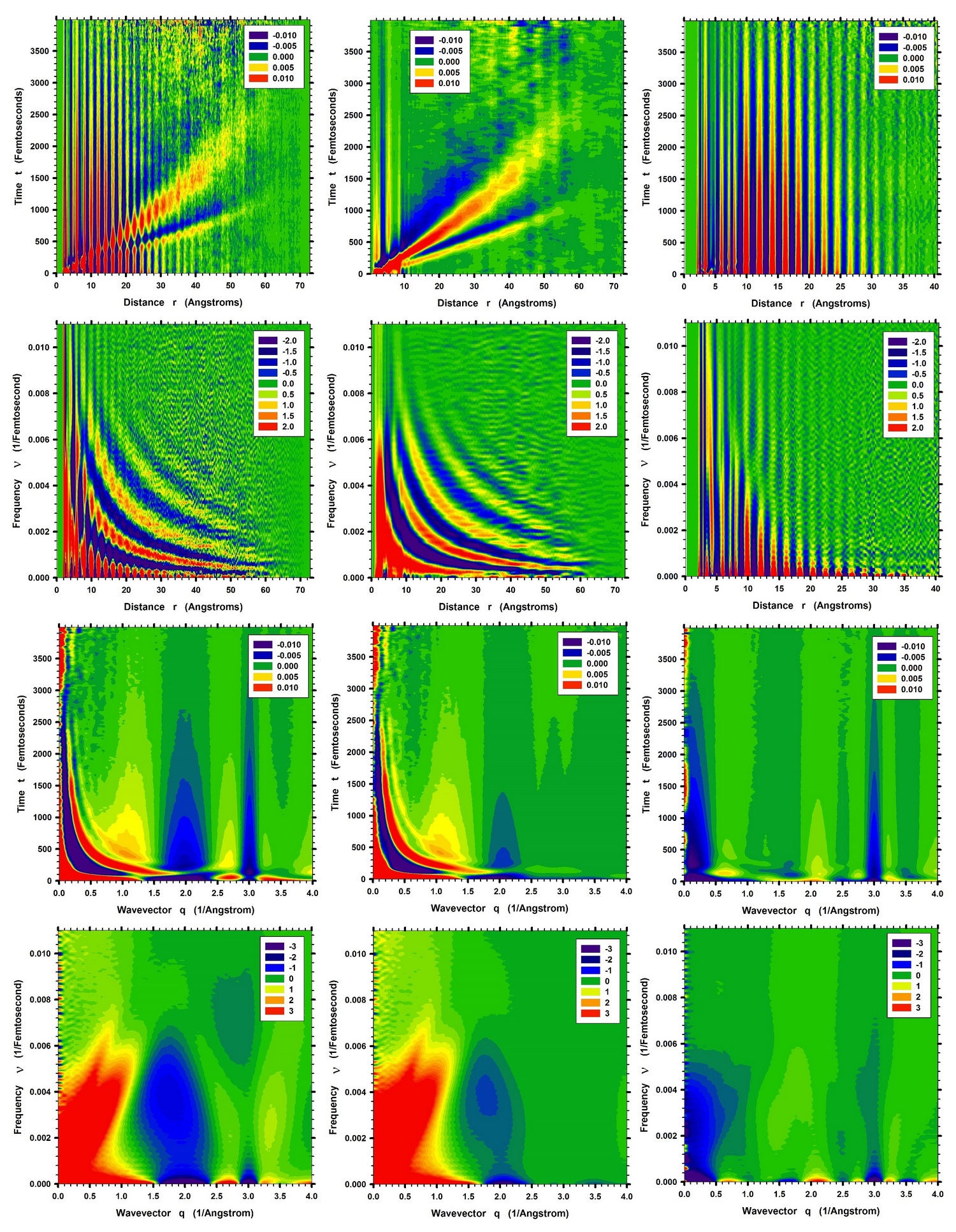
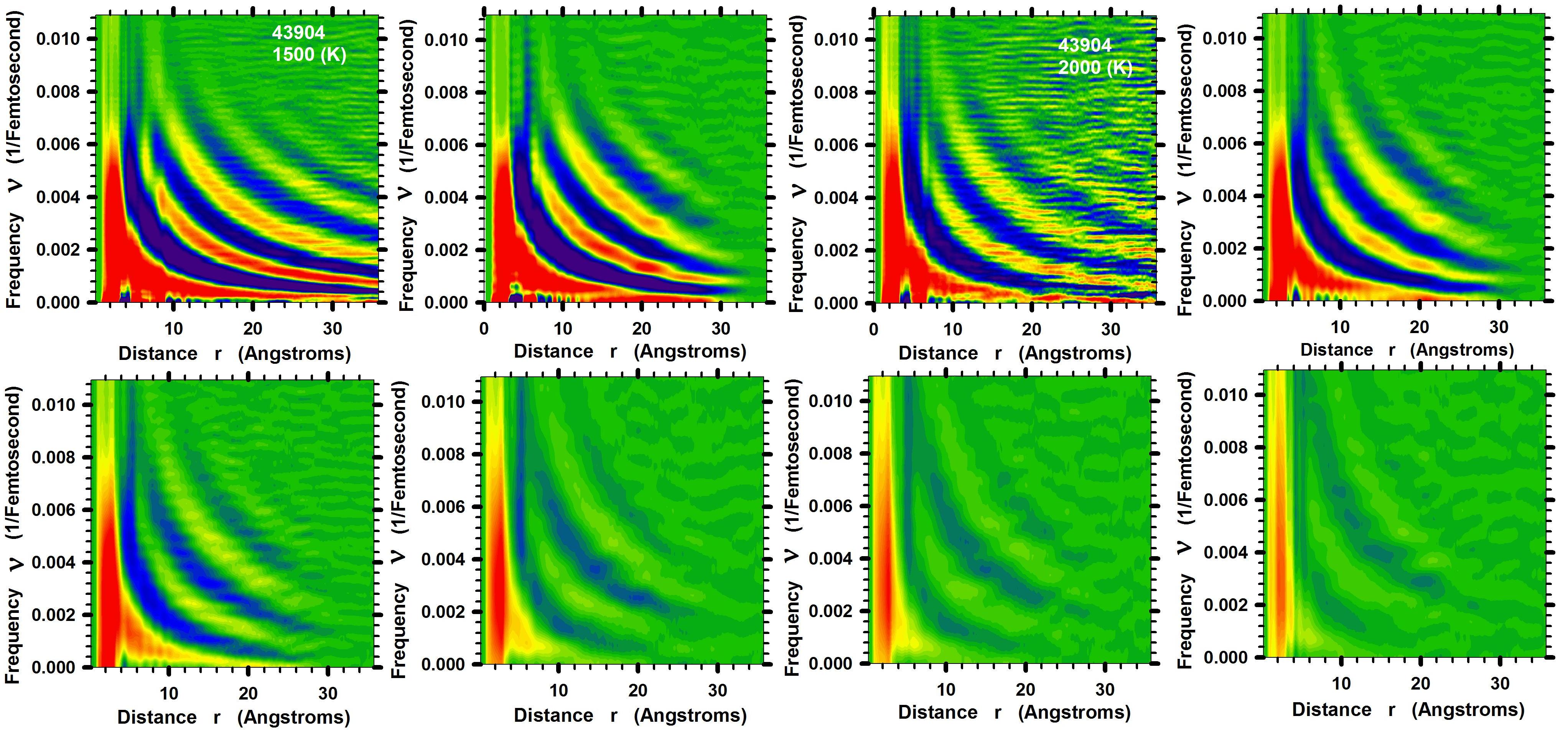
Panel (1,1) of Fig.1 shows the sscf  at 1500 (K) obtained on the large system of 43904 particles with $(L/2)\approx 41.21$ (Å) Levashov2013 , where $L$ is the length of the side of the cubic box. The main features present in the sscf  are the stress waves and the pair distribution function pdf -like stripe structure. To understand the results of the Fourier transforms of this panel, it is convenient to make an approximate separation of the sscf  into the parts that correspond to the waves and to the pdf -like structure.

The implemented separation procedure is based on the following observation. Consider the zero-time cut of panel (1,1) of Fig. 1. This cut is shown as the lowest curve in Fig.6 of Ref.Levashov2013 . Note the oscillating behavior for the distances beyond 10 (A). Also note that for a particular maximum, which is beyond 10 Å, the distances from it to the nearest two minimums are approximately the same. Thus, for a particular maximum at $r$ the value of the sscf  at it, $f_{gr}(r)$, could be approximated as:

$$f_{gr}(r)\approx-\frac{1}{2}\left[f_{gr}(r-\Delta_{r})+f_{gr}(r+\Delta_{r})\right]\;\;,$$ (1)

where $f_{gr}(r-\Delta_{r})$ and $f_{gr}(r+\Delta_{r})$ are the values of the sscf  at the left and right minimums nearest to this maximum. Finally, note that (1) can be used not only for the maximum/minimum values, but essentially for all $r$ beyond the third or forth coordination shells. This, however, does not hold for nonzero times and those regions of $r$ that contain contributions from the waves, as can be seen in Fig.2(a).

Further, we assume that the pdf -like contribution to the sscf  satisfies (1), while the wave’s contribution does not. In our iterative numerical procedure we consider different times independently. We assume that for a particular time we know the distance dependence of the wave contribution on step $n$, i.e., $\bar{f}^{n}_{w}(r)$. On the first step we assume that it is zero for all distances. Then we calculate the pdf -like contribution to the sscf  :

$$f_{gr}^{n}(r)=f(r)-\bar{f}^{n}_{w}(r)\;\;.$$ (2)

Then, in accord with (1), we define:

$$f_{gr}^{n+1}(r)=-\frac{1}{2}\left[f_{gr}^{n}(r-\Delta_{r})+f_{gr}^{n}(r+\Delta_{r})\right]\;\;,$$ (3)

where $\Delta_{r}$ is the distance from the nearest maximum to its nearest minimum. $\Delta_{r}$ is distance dependent (this dependence is weak in practice). Then we define the contribution from the wave on step $n+1$ as:

$$f_{w}^{n+1}(r)=f(r)-f_{gr}^{n+1}(r)\;\;.$$ (4)

Finally, we assume that the amplitude of the wave does not change significantly over the distance between the nearest maximum and minimum. It is indeed so according to Fig.2. Thus, for convergence of the algorithm, we introduce the average amplitude of the wave, $\bar{f}_{w}^{n+1}$, in which the averaging goes over the interval $(r-\Delta_{w},r+\Delta_{w})$:

$$\bar{f}_{w}^{n+1}(r)=\frac{1}{2\Delta_{w}}\int_{r-\Delta_{w}}^{r+\Delta_{w}}f_{w}^{n+1}(\xi)d\xi\;\;$$ (5)

With this new value of $\bar{f}_{w}^{n+1}(r)$ we go back to (2) closing the iteration loop.

Figure 3: Constant $r$ cuts of panel (1,2). The legends show the values of $r$. The curves were shifted so that they do not overlap. The first peaks in the curves are due to the compression wave, while the second peaks are due to the shear wave. Note that the shear peaks are larger and broader. The scale on the $y$-axis, corresponds to the correlation between the central atom and atoms in the spherical annulus of radius $r$ and thickness $dr=0.2$ (Å). Normalization to the atomic stress auto-correlation functions was also made.

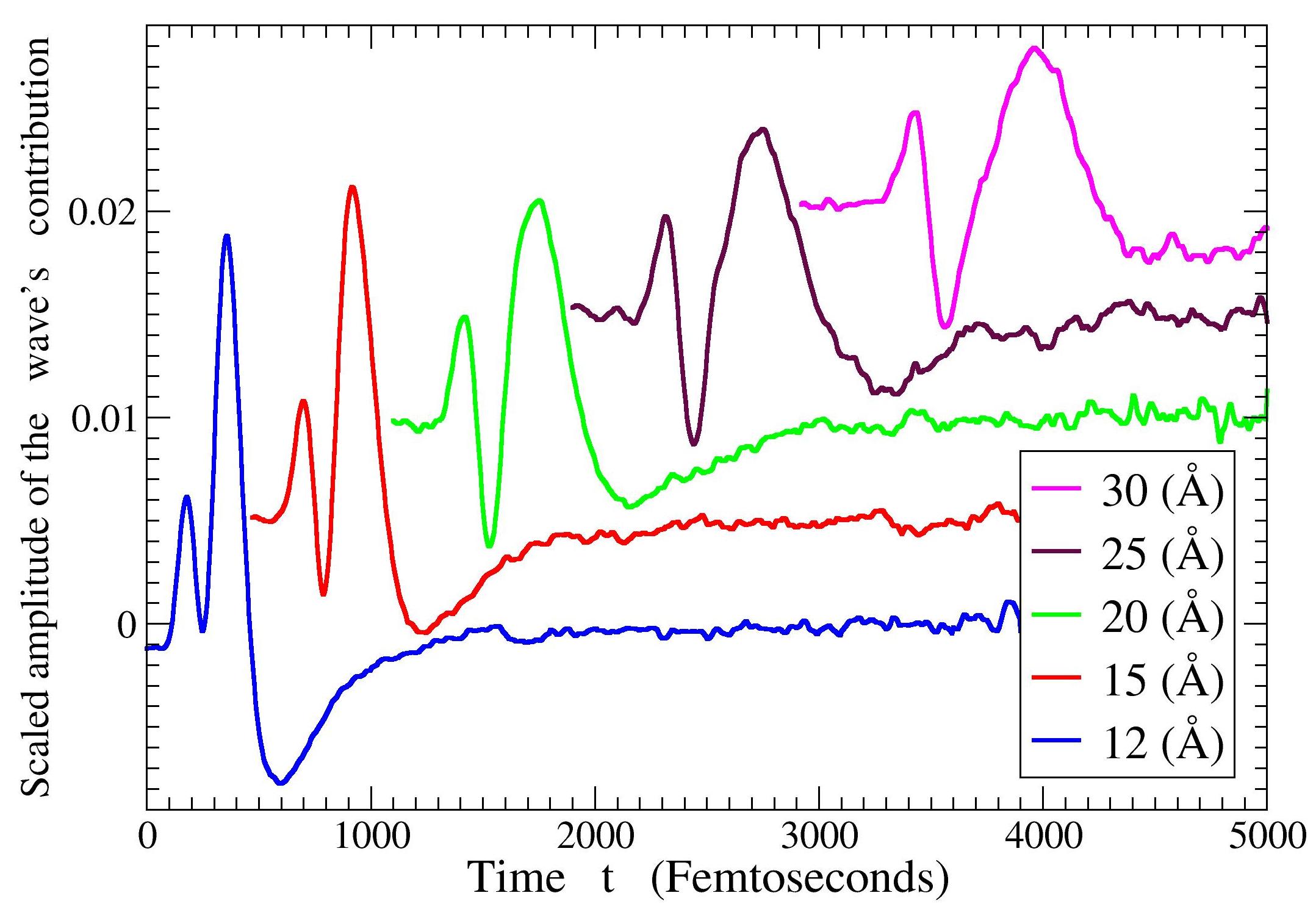
The results of the described procedure are shown in Fig.2 for temperature 1500 (K) and for the time-cut 500 (fs). The values of $\Delta_{r}$ were extracted from zero-time cuts of the sscf  , while the value used for $\Delta_{w}=1$ (Å). The number of iterations was 1000.

Note that the procedure does not work for distances $r<10$ (Å). This is so because for such $r$ in the pdf -like contribution there is no periodicity assumed in the separation procedure. The value of $r=10$ (Å) approximately corresponds to the inclusion of the 4th coordination shell. This distance could be associated with the medium range order distance Sokolov19921 ; Tomida19951 . It is of interest that viscoelastic continuous approximations appear to be valid at distances larger than $10$ (Å), but not at smaller distances Mizuno2013 .

We applied the described algorithm to all times in panel (1,1) of Fig.1. The results are shown in panels (1,2) and (1,3). Note again that the procedure does not work for $r<10$ (Å). Figure 3 shows constant $r$ cuts from panel (1,2). First peaks in the curves correspond to the compression wave, the second peaks to the shear wave. It would be useful to develop a method that would allow us separate contributions from the shear and compression waves.

IV What we see in panels
(1,1), (1,2), and (1,3)

The intensity in panel (1,1) of Fig.1 shows the ensemble averaged atomic level stress correlation function between a central atom and atoms located inside the spherical annulus of radius $r$ and thickness $\Delta r=0.2$ (Å). This intensity is also normalized to the magnitude of the stress auto-correlation function at zero time Levashov20111 ; Levashov2013 . Figures 6 and 7 of Ref.Levashov2013 , and Figures 2,3 of this paper further clarify the scale of the correlations. For example, the magnitude of the stress correlation of a central atom with the maximum intensity annulus in the first coordination shell at zero time is $\sim 0.35$ of the stress auto-correlation function at zero time (width of the annulus is $\Delta r=0.2$ (Å)). For the maximum intensity annulus in the second coordination shell this ratio is less than $0.10$ (from Fig.6 of Ref.Levashov2013 ). It is also useful to recall that the value of the stress auto-correlation function at zero time determines the value of the atomic level stress energy Egami19821 ; Chen19881 ; Levashov2008B .

Figure 4: Dependencies on time of the stripes’ maximums in the pdf -like contribution to the sscf  . See panel (1.3) of Fig.1. The legends show the positions of the stripes. The figure and the inset show the same data. Linear behavior of the curves in the inset at large times suggests a relation between the decay of the maximums of the stripes and diffusion.

Panels (1,1), (1,2), and (1,3) raise several questions. For example, as panel (1,1) shows the atomic level decomposition of the macroscopic shear sscf  $\left<S^{xy}S^{xy}\right>$, it is reasonable to wonder why we see in it the pdf -like structure and the contributions from the longitudinal waves. Indeed, both of these features should be related to the density fluctuations and not to the shear sscf  . The explanation can be related to the results presented in Ref.Kust2003a ; Kust2003b . There it was shown that different components of the atomic level stress tensor on the same atom are correlated. On the other hand, the presence of correlations between the different stress components on the same atom questions the results and derivations in Ref.Egami19821 ; Chen19881 ; Levashov2008B , as there, when the equipartition law is derived, it is assumed that different stress components on the same atom are independent. However, the derivations of the equipartition in Egami19821 ; Chen19881 ; Levashov2008B are based on the Taylor expansion and considerations of only those terms which are quadratic in atomic strain. Under this quadratic approximation, different stress components on the same atom are independent in the spherical (cubic) representation. Thus, the results presented in Ref.Kust2003a ; Kust2003b can be related to the higher order terms in the Taylor expansion. This means that the density-density correlations which we see in panels (1,1), (1,2), and (1,3) can be related to higher order terms. These questions require further clarifications.

IV.1 pdf -like contribution

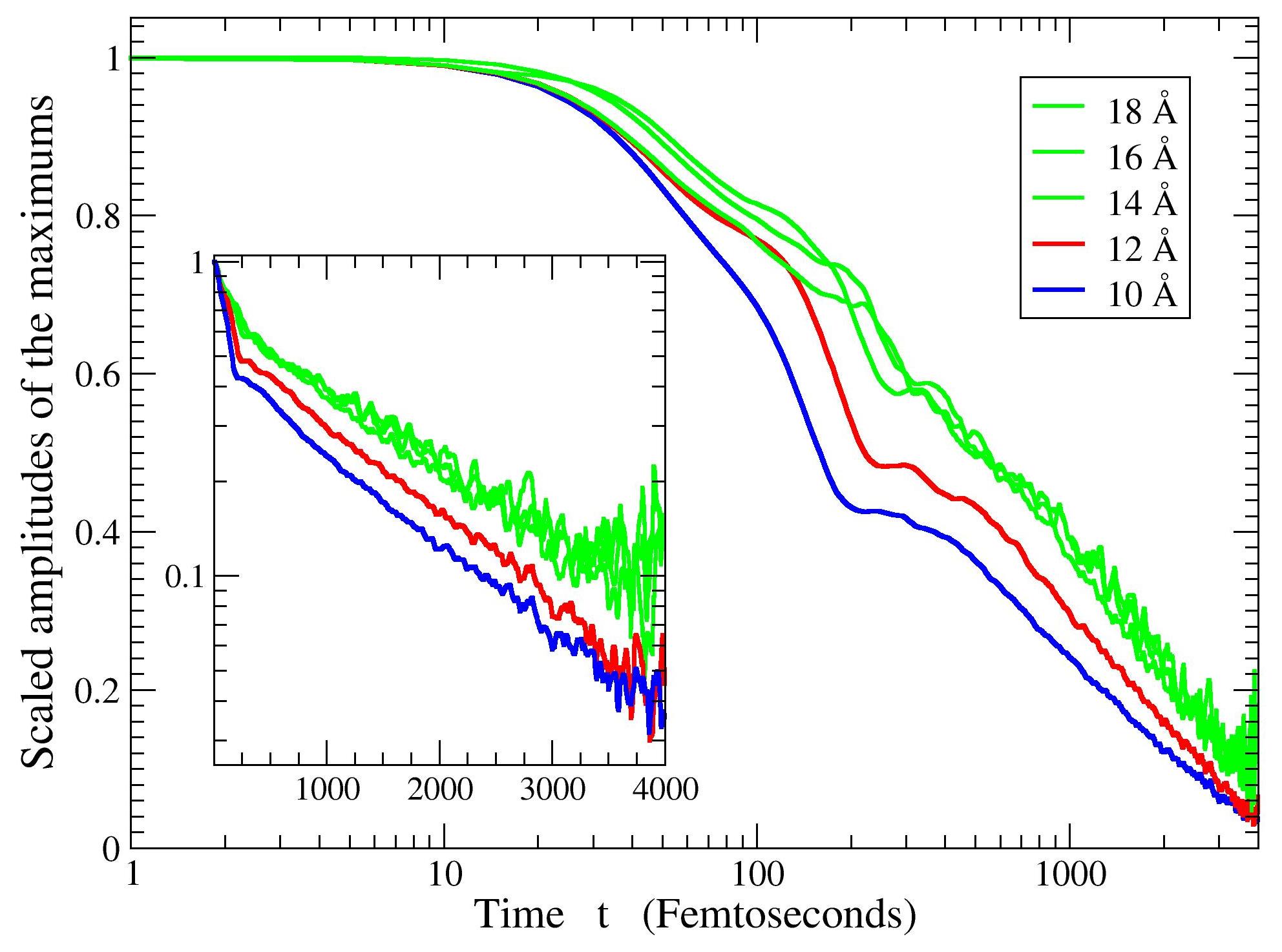
It is reasonable to expect that the decay of the pdf -like contribution in panel (1,3) is related to the decay of the van Hove correlation function vanHove . Figure 4 shows dependencies on time of the maximums in the pdf -like contribution to the sscf  . For example, 12 (Å) maximum was found as the maximum value (for every time) of the pdf -like contribution in the interval of distances between 11 (Å) and 13 (Å). Differences between the 10 (Å), 12 (Å) and the other curves are likely to be caused by the stress waves: as intensities of the stress waves are larger at small distances it is likely that these higher intensities stimulate faster decay in the pdf -like stripes. The decay in the amplitudes of the stripes for $t<200$ (fs) is likely to be due to the rattling cage motion. The decay for $t>300$ (fs) is likely to be related to the particle diffusion. If we assume that the particles that diffuse away from the spherical annulus completely lose the correlation with the original state, while those that remain keep this correlation, then the magnitude of the remaining correlation should be proportional to the number of the particles remaining in the annulus. Since the rate of diffusion away from the spherical annulus should be proportional to the number of particles remaining in the annulus, the number of the remaining particles should decrease exponentially with time. Thus the pdf -like stress correlation function at large distances at $t>300$ (fs) should decay exponentially with time. This behavior can be observed in the inset of Fig.4.

IV.2 Stress waves’ contribution

It is clear that panel (1,2) shows propagating shear and compression waves. Previously we argued that shear stress waves are related to viscosity Levashov20111 ; Levashov2013 . Thus, it is important to understand the features in panel (1,2). However, it is not clear how stress waves translate into the features observed in the sscf  . The nature of these stress waves also remains obscure. These are complicated questions for liquids, as currently there is no accepted and convenient way to describe vibrational dynamics in disordered media and its coupling to diffusion Keyes19971 ; Taraskin20001 ; Taraskin20021 ; Ediger20121 ; Tan20121 . In our view, it is possible that the atomic level stress correlation function that we consider here represents an alternative way to describe vibrational dynamics.

In order to gain at least some insight into the connection between the vibrational dynamics and the atomic level stress correlation function we considered in Ref.Levashov20141 a simple model. In this model vibrational modes are represented by plane waves, like in crystals. Of course, plane waves do not represent vibrational eigenmodes of liquids Taraskin20021 ; Ediger20121 ; Keyes19971 ; Taraskin20001 ; Tan20121 . However, in our view, considerations in Ref.Levashov20141 provide insight into the nature of the connection between the stress waves and the atomic level stress correlation function.

V Fourier Transforms of the sscf  

In our previous considerations, the atomic level sscf  , $F(t,r)$, is defined as a correlation function between a central atom and atoms inside the spherical annulus of radius $r$ and thickness $dr$ Levashov20111 ; Levashov2013 . This definition naturally follows from the Green-Kubo expression for viscosity. For further analysis and in view of Ref.Levashov20141 we introduce:

$$f_{p}(t,r)\equiv\frac{1}{(4\pi r^{2})}F(t,r)\;,\;\;\;\;\;f_{r}(t,r)\equiv r\cdot f_{p}(t,r)\;\;,\;\;\;$$ (6)

where $f_{p}(t,r)$ is the atomic level stress correlation per pair of particles.

We define the Fourier transform over $t$ of $f_{r}(t,r)$ as:

$$\tilde{f}_{r}(\omega,r)\equiv\int_{0}^{\infty}f_{r}(t,r)\cos(\omega t)dt\;\;.$$ (7)

It was shown, in the framework of the model discussed in Ref.Levashov20141 , that if vibrations are non-decaying plane waves, then $\tilde{f}_{r}(\omega,r)$ should, for every $\omega$, exhibit constant amplitude oscillations in $r$ with a wavelength determined by the dispersion relation $\omega(q)$. Since, for different $r$ the Fourier transforms over $t$ are independent, we transform $F(t,r)$ instead of $f_{r}(t,r)$. In the case of non-decaying plane waves, amplitudes of peaks in $\tilde{F}(\omega,r)$ should linearly increase with increase of $r$.

We define the Fourier transform over $r$ of $f_{r}(t,r)$ as:

$$\tilde{f}_{r}(t,q)\equiv\int f_{r}(t,r)\sin(qr)dr\;\;.$$ (8)

As shown in Ref.Levashov20141 , $\tilde{f}_{r}(t,q)$ for non-decaying plane waves should exhibit constant amplitude oscillations in $t$ with a period determined by the dispersion relation.

Equation (8) can also be rationalized from a different perspective. It is natural to assume that the stress correlation function for a particular pair of atoms, i.e., $f_{p}(t,\bm{r})$, depends on the direction of the radius vector, $\bm{r}$, from one atom to another. Let us define the three-dimensional Fourier transform of this stress correlation function as it is usually done:

$$\tilde{f}_{p}(t,\bm{q})\equiv\int f_{p}(t,\bm{r})\exp(\;-i\bm{q}\bm{r}\;)d\bm{r}\;\;.$$ (9)

In isotropic cases, $f_{p}(t,\bm{r})\equiv f_{p}(t,r)$ and (9) could be rewritten as:

$$\left[q\,\tilde{f}_{p}(t,q)\right]\equiv\int\left[r\,f_{p}(t,r)\right]\sin(qr)dr\;\;.$$ (10)

It follows from (6) that expression (10) is equivalent to expression (8). The expression (10) is similar to the expression that connects the pair distribution function, to the reduced scattering intensity Warren .

The Fourier transform in time-space naturally follows from the formulas (7,8). It was shown in Ref.Levashov20141 , in the frame of the model considered there, that the Fourier transform of $f_{r}(t,r)$ over $t$ and $r$ should lead to the dispersion curves.

VI Results of the Fourier Transforms at 1500 K

Since $F(t,r)$ was obtained in MD simulations on systems of finite sizes with periodic boundary conditions there is a lower limit on the possible values of $q$ that we can consider. See Ref.qmin for details.

VI.1 Time to frequency Fourier transform

The second row of Fig.1 shows $\tilde{F}(\omega,r)$, i.e., time to frequency Fourier transforms (7) of $F(t,r)$ and contributions to it from the wave -like and the pdf -like parts. Panels (2,1), (2,2), (2,3) were obtained from the data in panels (1,1), (1,2), (1,3) respectively.

In panel (2,2) contributions from the shear and compression waves are mixed. For an analysis of the stress waves it would be very useful to find a way to separate contributions from these waves. Since the amplitude of the compression wave in panel (1,2) is significantly smaller than the amplitude of the shear wave, it is reasonable to assume that features in the upper panels of Fig.5 are dominated by the shear waves.

It is useful to compare panel (2,2) of Fig.1 of this paper with panel (1,2) of Fig.7 in Ref.Levashov20141 . Note, however, that panel (2,2) of Fig.1 shows $t$ to $\omega$ Fourier transform of the function $r^{2}f_{p}(t,r)$, while panel (1,2) of Fig.7 in Ref.Levashov20141 shows the Fourier transform of the function $rf_{p}(t,r)$. We show in this paper the Fourier transform of $r^{2}f_{p}(t,r)$ because it is more directly related to the generalized viscosity and also because in Fig.5 this $r^{2}$-scaling allows showing relative amplitudes of the peaks in $\tilde{F}(\omega,r)$ more clearly.

Figure 5 shows constant $\omega$-cuts of panel (2,2). If in panel (2,2) there were only shear waves, then, according to Ref.Levashov20141 , for every $\omega$ in Fig.5 the period of oscillations in $r$ would give the wavelength that corresponds to this value of $\omega$. If the sscf  were caused by non-decaying plane waves, then the amplitudes of the peaks in Fig.5 would linearly increase with increase of $r$. However, the amplitudes of the peaks in Fig.5 decrease with increase of $r$. This behavior suggests that the dynamic underlying the behavior of $F(t,r)$ is very different from the vibrational dynamics of non-decaying plane waves.

The lower panel in Fig.5 shows the dependence of wavevector on frequency determined from the two upper panels. This dependence should primarily correspond to the dispersion relation for the shear waves. Indeed, the slope of the curves corresponds to the speed $\approx 3$ (km/s), i.e., to the shear waves, according to panel (2,2) of Fig.1. Still, this picture should contain certain distortions due to the compression waves.

Figure 5: Constant $\omega$ cuts from panel (2,2). Legends show the values of $\omega$. The blue curves in upper two panels show the result from the large system with $(L/2)\approx 41.2$ (Å). Green curves show the results from the system with $(L/2)\approx 20.6$ (Å). We use the positions of the maximums and minimums, marked by the red squares, to determine the wavelengths, $\lambda=2\pi/q$. Lower horizontal panel shows the dependence of $q$ on $\omega$. Different curves in the lower panel correspond to different selections of red squares used for the determination of wavelength. For example, the notation (2,4) corresponds to the selection of the second and the forth squares from the left to determine the wavelength.

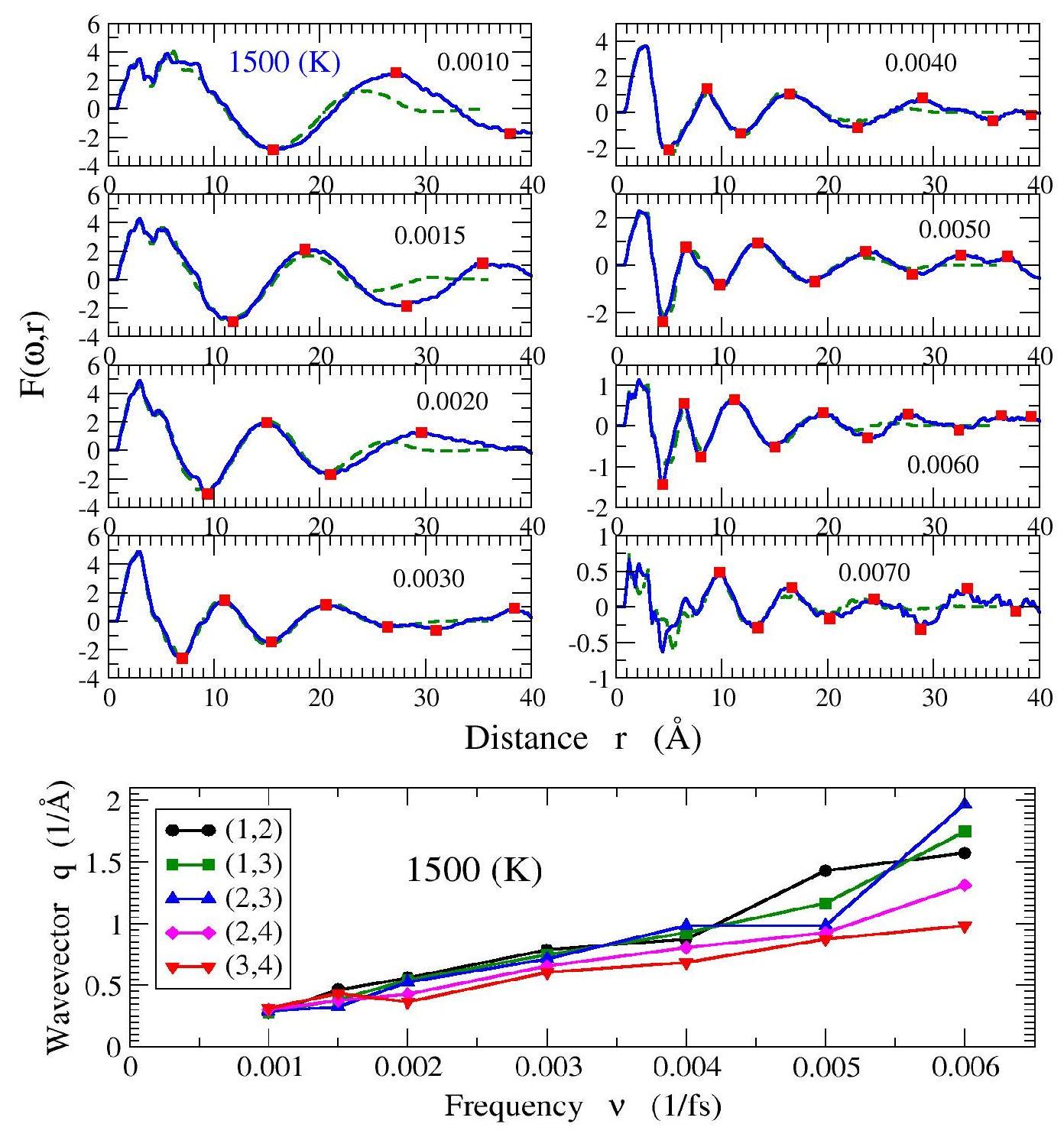
By comparing the scales on the $y$-axes in the upper panels of Figure 5, note that the amplitudes of the waves for higher frequencies are significantly smaller than the amplitudes for lower frequencies. Note also that, even for the highest frequencies shown, the waves propagate over, at least, 5 interatomic spacings ($r_{nn}\approx 2.6$ (Å)). In this context the following comment is relevant. It can be seen in panel (1,2) of Fig.1 and in Fig.3 that the feature corresponding to the compression waves is not just smaller in the amplitude than the feature corresponding to the shear waves, but it is also narrower in $t$ and in $r$. Since it is narrower in $t$ its Fourier transform over time decays in a wider range of frequencies. Thus contributions from the compression waves to the higher frequency curves in Fig.5 should be relatively larger than to the lower frequency curves. Because of the overlap of contributions from the compression and shear waves, we do not discuss here attenuation rates for different frequencies.

In considerations of the macroscopic (tccf  ) it is assumed that only transverse waves contribute to it HansenJP20061 ; Boon19911 ; EvansDJ19901 ; Levesque19731 ; EvansDJ19811 ; Alder19831 ; Mountain19821 ; PalmerBJ19941 ; Kaufman2007E ; Puscasu110 ; Tanaka20091 ; Tanaka2011E ; Furukawa2013E ; Mizuno2012 ; Mizuno2013 . However, in view of the results discussed above, it is likely that compression waves also affect the tccf  . Thus the results obtained from the analysis of the tccf  can be distorted by the compression waves. While the distortions should not be very significant this issue deserves attention and clarification.

It follows from panel (2,2) of Fig.1 that the main sickle  feature vanishes at large distances because of the finite system size. This effect can also be seen in Fig. 12. Thus, periodic boundary conditions (PBC  ) affect the stress waves of small frequencies, i.e., $\nu\approx 0.0005-0.001$ (fs^-1). It is shown in section (C) that contributions from the shear and compression waves overlap in the main sickle  feature.

Flattening of the main sickle  feature at low temperatures in the region of frequencies between 0.001 and 0.002 (fs^-1) means that the stress waves of the lower frequencies can propagate over large distances. Frequency $\nu=0.001$ (fs^-1) corresponds to the energy $h\nu\approx 4.1$ (meV). This energy approximately corresponds to the energy of the boson peak in metallic glasses Ruocco20131 ; Ediger20121 . Thus significant increase of the propagation range with decrease of temperature happens in the range of frequencies usually associated with the boson peak. In a recent review Ediger20121 it was stated, on the basis of Ref.Taraskin20021 ; Tanaka20081 , that: “There appears to be a growing consensus that the frequency of the boson peak corresponds to the maximum frequency at which transverse phonons can propagate in the disordered material …” Our data are in agreement with this statement.

In panel (2,3) seemingly faster decay of the vertical stripes at large distances is misleading. Perceived behavior originates simply from the smaller amplitudes of the stripes at large distances at zero time. According to Fig.4 at large distances all stripes decay at the same rate.

VII Frequency dependent viscosity

According to formulas (18-22) in the Appendix A viscosity is a complex function of the wavevector $\bm{k}$ and frequency $\omega$. The stress correlation function is a complex function of $\bm{k}$ and time. All results presented in this paper have been obtained for $\bm{k}=0$. In this case the components of the stress tensor and their correlation functions are real quantities (20,21,22,24). However, viscosity remains a complex function of $\omega$ (23): $\eta(\omega)\equiv\eta^{\prime}(\omega)-i\eta^{\prime\prime}(\omega)$. Complex viscosity is related to the complex shear modulus: $G(\omega)=G^{\prime}(\omega)+iG^{\prime\prime}(\omega)=i\omega\eta(\omega)$ Bland . Thus the real part of viscosity describes energy dissipation in liquids, while the imaginary part describes elastic response.

It follows from the previous definitions of $\eta(\omega)$ HansenJP20061 ; Boon19911 ; EvansDJ19901 ; Kaufman2007E and our definitions Levashov2013 ; Levashov20111 that:

$$\eta^{\prime}(\omega)=\frac{\rho_{o}}{k_{b}T}\int_{0}^{t_{max}}\left\{\int_{0}^{R_{max}}F(t,r)dr\right\}\cos(\omega t)\,dt\;\;\;.$$ (11)

Or:

$$\eta^{\prime}(\omega)=\frac{\rho_{o}}{k_{b}T}\int_{0}^{R_{max}}\tilde{F}(\omega,r)dr\;\;\;.$$ (12)

Thus, for every $\omega$ in panel (2,1) of Fig.1 the integral over $r$ gives $\eta^{\prime}(\omega)$. Integration over a range of distances, $(r_{1},r_{2})$, should allow estimation of how this range contributes to $\eta^{\prime}(\omega)$.

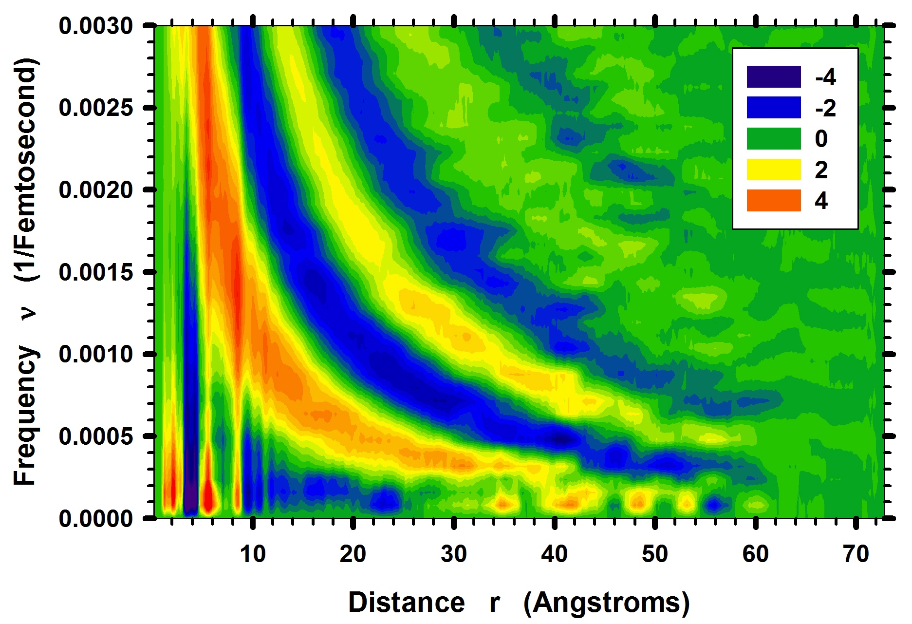
According to formula (23) the imaginary part of viscosity can be calculated with $\sin(\omega t)$ instead of $\cos(\omega t)$ in (11). Figure 6 shows $\sin(\omega t)$ Fourier transform of the panel (1,2) of Fig.1 in the region of smaller frequencies. For every $\omega$ in Fig.6 the integral over $r$ gives the imaginary part of viscosity, i.e., $\eta^{\prime\prime}(\omega)$. We will see further that the most interesting behavior happens in the region $\omega<0.0010$ (1/fs).

Figure 6: Fourier transform of the data in panel (1,2) of Fig.1 through $\sin(\omega t)$. This figure is very similar to panel (2,2) of Fig.1. However, it is a different figure. For every $\omega$ the integral over $r$ gives the imaginary part of viscosity, i.e., $\eta^{\prime\prime}(\omega)$. The largest time up to which we calculated the sscf  in our simulations was 4000 (fs). Thus we should not consider frequencies smaller than $1/4000$ (1/fs) or $0.00025$ (1/fs).

It is known that the real part of the frequency dependent viscosity, $\eta^{\prime}(\omega)$, exhibits on decrease of temperature frequency dependent increase Alder19831 ; Kaufman2007E ; Tanaka20091 ; Donko20101 . This increase is the most significant for small $\omega$. Considerations of our results in this context provide additional insights into this phenomena.

The statistics of our data for the atomic level sscf  is not sufficient to consider in detail low frequency behavior of the macroscopic viscosity due to the cross  term. However, the macroscopic sscf  due to the cross  term can also be obtained as a difference between the total  sscf  function and the self  term of the sscf  . In Ref.Levashov2013 we considered the behaviors of the total  sscfs  and their self  terms at different temperatures. The differences between the total  sscfs  and their self  terms are shown in Fig.7.

Figure 7: Normalized cross  sscfs  at different temperatures. In the inset the blue curve shows the results of integration over $r$ of the data in panel (1,1) of Fig.1. The orange curve in the inset was obtained on the intermediate size system as a difference between the total  sscf  and the self  term of the sscf  Levashov2013 . The black curve at short times is the orange curve. For times $t>230$ (fs) the black curve was fitted to the reliable part of the simulation data and then the fitted curve was used as an approximation when the simulation data become unreliable fitdiff . The curves in the main plot show the results of MD simulations at short times and the fitted curves at large times fitdiff .

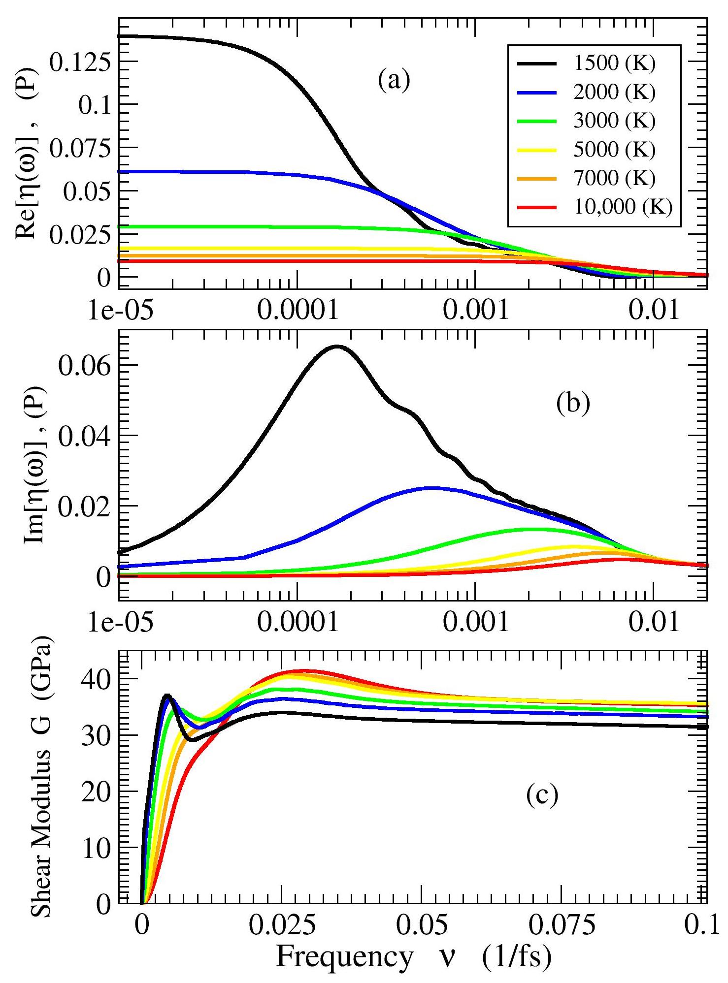
Panels (a) and (b) of Fig.8 show how the real and imaginary parts of viscosity due to the cross  term depend on frequency. The curves in these panels were obtained by $\cos(\omega t)$ and $\sin(\omega t)$ integrations of the cross  sscf  curves in Fig.7. The viscosity curves exhibit expected behaviors. The rise in the value of the real part of viscosity at low frequencies was reported many times previously Alder19831 ; Kaufman2007E ; Tanaka20091 ; Donko20101 . The presence of the peak in the imaginary part of viscosity is also well known Bland ; Donko20121 ; Maggi2008 .

Panel (c) shows the real part of the frequency dependent shear modulus, i.e., $G^{\prime}(\omega)=\omega\eta^{\prime\prime}(\omega)$. In the limit of large frequencies the curves exhibit expected saturation to the infinite frequency value. Infinite frequency shear modulus for fcc iron is $\sim 80$ (GPa) EightyGPa . From Fig.8 we get the value $\sim 30$ (GPa). This happens because we consider the contribution from the cross  term only. The value of the shear modulus increases with increase of temperature because the data has been obtained in constant volume simulations.

New insights come from the comparisons of the regions in $\omega$ where $\eta^{\prime}(w)$ and $\eta^{\prime\prime}(\omega)$ start to increase from their large-$\omega$ values with the corresponding $\omega$-regions in panel (2,2) of Fig.1 and in Fig.6. These comparisons suggest that the increase in the ranges of propagation of the shear stress waves correlates with the increase in the values of the real and imaginary parts of viscosity. For $\eta^{\prime\prime}(\omega)$ the increase is related to the sickle feature in Fig.6 which is the closest to the origin. We again note that we should not consider frequencies $\omega<0.00025$ (1/fs) on the basis of Fig.1 and Fig.6 since corresponding simulations were not long enough.

Figure 8: Panel (a) shows the dependencies of $\eta^{\prime}(\omega)$ on $\omega$ at different temperatures. The curves were obtained through $\cos(\omega t)$ integration of the curves in Fig.7. Note that increase in the value of $\eta^{\prime}(\omega)$ on decrease of temperature is the most significant for low frequencies. This increase correlates with increase in the ranges of propagation of the shear waves of low frequencies on decrease of temperature. Panel (b) shows dependencies of $\eta^{\prime\prime}(\omega)$ on $\omega$. Panel (c) shows dependencies of the real part of the shear modulus, i.e. $\omega\eta^{\prime\prime}(\omega)$, on $\omega$ at different temperatures. Note that the scale on $\omega$-axis in (c) is different from $\omega$-scales in (a) and (b).

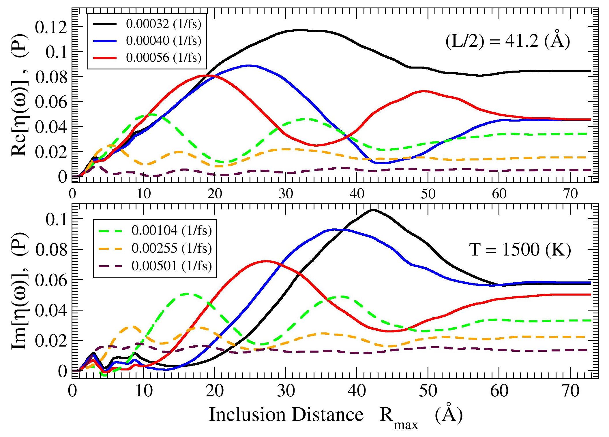
In order to demonstrate the connection between the propagation of the shear waves and viscosity further we show in panel (a) of Fig.9 how $\eta^{\prime}(\omega,R_{max})\equiv\int_{0}^{R_{max}}\tilde{F}(\omega,r)dr$ depends on $R_{max}$ for the selected values of $\omega$ shown in the legends. Panel (b) is similar to panel (a), but it is for $\eta^{\prime\prime}(\omega,R_{max})$. The shapes of the curves suggest/demonstrate that the microscopic origin of viscosity is related to the propagation and dissipation of the shear waves on atomic scale.

Figure 9: Dependencies of $\eta^{\prime}(\omega,R_{max})$ and $\eta^{\prime\prime}(\omega,R_{max})$ on the inclusion distance $R_{max}$. The curves for $\eta^{\prime}(\omega,R_{max})$ in panel (a) were obtained by integration over $r$ of the constant $\omega$-cuts from panel (2,2) of Fig.1. The curves for $\eta^{\prime\prime}(\omega,R_{max})$ in panel (b) were obtained by integration over $r$ of the constant $\omega$-cuts from Fig.6. The macroscopic values of the viscosities correspond to the values to which the curves converge at large $R_{max}$. The selected frequencies are the same in both panels. The legends in panel (a) give the values of $\omega$ for the solid curves. The legends in panel (b) give the values of $\omega$ for the dashed curves. Note that all solid curves correspond to the values of $\omega<0.001$ (1/fs).

VII.1 Distance to wavevector Fourier transform

Panels (3,1), (3,2), (3,3) show $r$ to $q$ Fourier transforms (8) of the function $f_{r}(t,r)=rf_{p}(t,r)$ obtained from the data in panels (1,1), (1,2), (1,3) respectively. It is useful to compare panel (3,2) with panel (2,1) of Fig.7 in Ref.Levashov20141 . In these two panels $r$-scalings are the same.

For every particular time, the Fourier transform (8) of the sscf  over $r$ is similar to the transform of the pair density function, $G(r)$, into the structure factor, $S(q)$; if $G(r)=4\pi r\left[\rho(r)-\rho_{o}\right]$ then $q\left[S(q)-1\right]=\int_{0}^{R_{max}}G(r)\,\sin(qr)\,dr$ Warren . Thus, knowledge of the general relations between $G(r)$ and $S(q)$ can help in guessing the roles of certain features. This parallel allows us to relate the negative intensity near 3 (Å^-1) in (3,3) to the periodicity in $r$ of the pdf -like contribution to the sscf  (see (1,3)). The width of the 3 (Å^-1) feature in (3,3) is related to the extend of the pdf -like oscillations in $r$.

Panels (3,1) and (3,2) show for how long in time stress waves, with a particular value of the wavevector, exist. If the stress waves were non-decaying plane waves, then, according to Ref. Levashov20141 , for every $q$ the amplitude of oscillations would be constant in time. Note that non-zero intensity for smaller $q$ exists for larger times than nonzero intensity for larger wavevectors. Recall that in panels (3,1) and (3,2) the contributions from the shear and compression waves overlap.

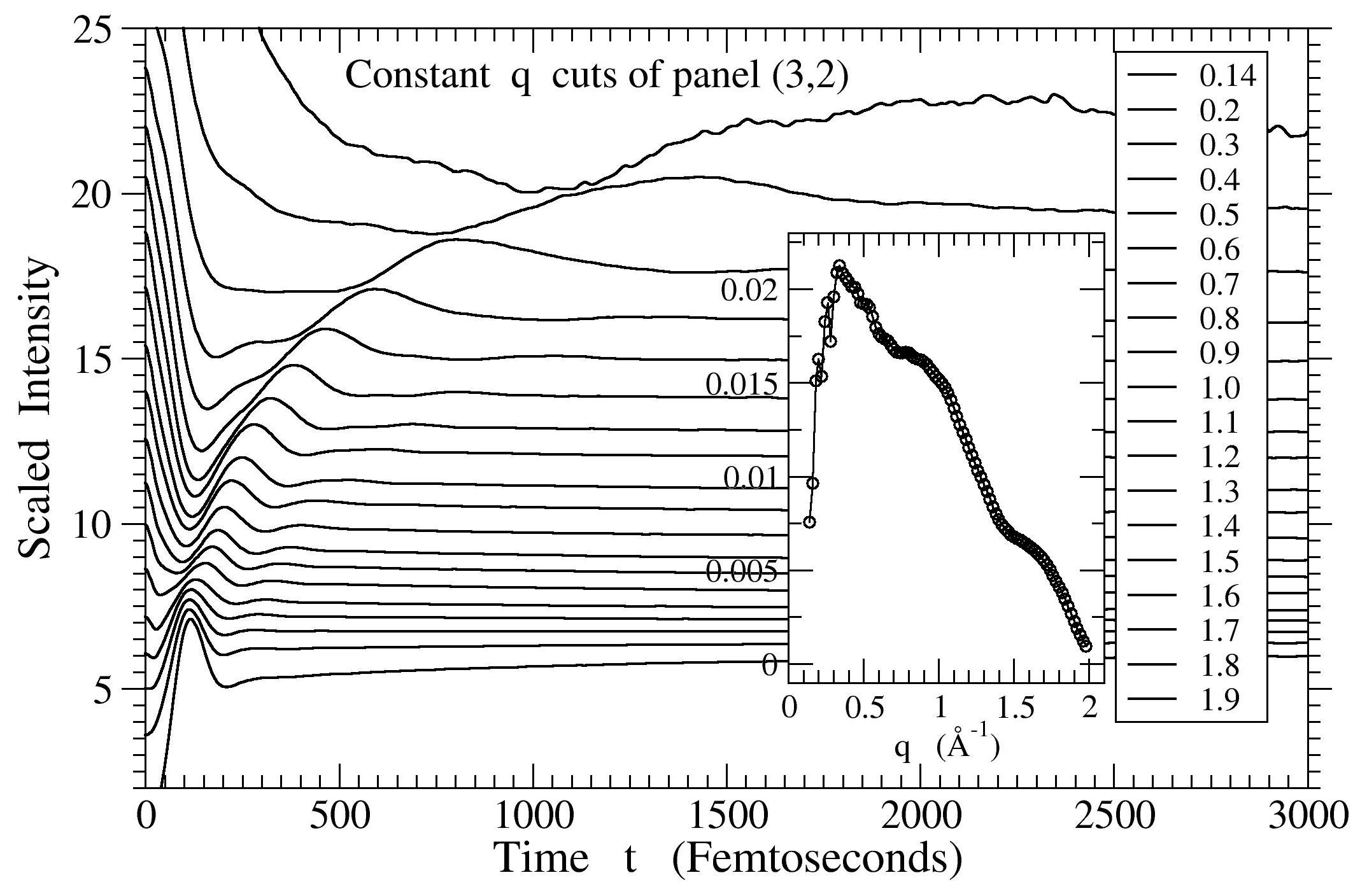
Figure 10 shows constant $q$ cuts of panel (3,2) of Fig.1. We see in Fig.10, as in panel (3,2), that for every $q$ there are no more than two oscillations in time, with the amplitude of the second maximum significantly smaller than the amplitude of the first maximum. Thus, the situation in the considered liquid at 1500 (K) is quite different from the situation in a model crystal with non-decaying vibrational plane waves Levashov20141 . In the model crystal the amplitudes of these oscillations should be constant in time. The relative intensities of the maximums in Fig.10 for different $q$ should be related to the relative vibrational densities of states and to the relative rates of decay for different $q$.

Figure 10: Normalized and shifted constant $q$ cuts of panel (3,2) of Fig.1. Every particular $q$-cut was scaled to the maximum intensity in the sickle  feature for this $q$ and then shifted. The dependence of this maximum intensity on $q$ is shown in the inset. Different curves correspond to the different values of $q$ (in Å^-1) given in the legends. Upper curves correspond to the upper legends.

Figure 11: The wave -like contributions to the sscf  at different temperatures on the systems of 43904 and 5488 particles. Panels (1,1) and (1,3) are for the 43904 particle system. All other panels are for the 5488 particle system. Panels (1,1) and (1,2) are for $T=1500$ (K). Panels (1,3) and (1,4) are for $T=2000$ (K). Panel (2,1) is for 3000 (K), (2,2) is for 5000 (K), (2,3) is for 7000 (K), (2,4) is for 10000 (K). Note in panels (1,1) and (1,2) bright vertical stripes at $r\sim 5$ (Å). These stripes show that the separation procedure used to produce wave -like contributions does not work for these distances. Note also that there are no such bright vertical stripes in the other panels. In the text we argue that this bright vertical stripe is the origin of the bonfire  feature in the (t,q)-sscf  .

Note that the main sickle  feature ends at $q_{wmax}\approx 1.75$ (Å^-1), i.e., at $\lambda_{wmin}=2\pi/q_{wmax}\approx 3.6$ (Å). Thus, $\lambda_{wmin}\approx 1.4d$, where $d$ is the average distance between the nearest particles for the chosen value of the density and also the equilibrium distances between a pair of particles for our potential. The fact that the smallest possible wavelength of the shear stress waves is $\approx 1.5\,d$ is in approximate agreement with the other results Alley19831 ; Mizuno2013 . In our data, the crossover in the main sickle  feature happens at $q_{c}\approx 0.5$ (Å^-1), i.e., at $\lambda_{c}\approx 12.6$ (Å) or $\approx 4.8d$. At larger distances, according to Ref.Mizuno2013 , ordinary hydrodynamics with $q$-independent transport coefficients is valid, while at smaller distances the situation is more complicated.

Figure 12: The sscf  in $(\omega,r)$-space for different systems and at different temperatures. The locations of panels correspond to those in Fig.11. The scales on the $z$-axes are the same as in panel (2,2) of Fig.1.

Figure 13: The sscf  in $(t,q)$-space for different systems and at different temperatures. The locations of panels correspond to those in Fig.11. Note that panels (1,1) and (1,2) contain the bonfire  feature, while the other panels do not. From comparisons with panels in Fig.11, it follows that the bonfire  feature is related to the bright vertical stripe at $r\approx 5$ (Å).

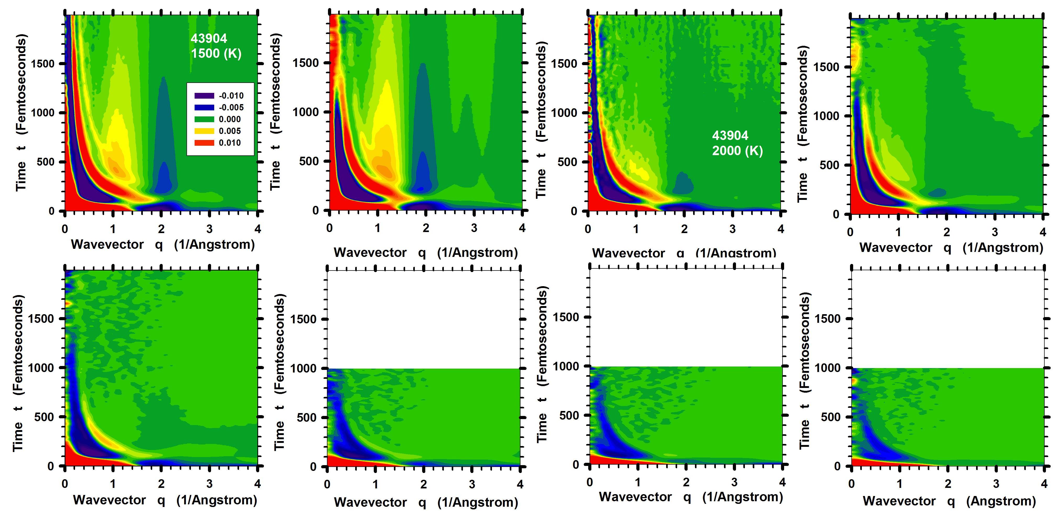
There are two features in panels (3,1) and (3,2) that we discuss in sections (B) and (C). The first feature is a positive intensity that is centered at $q\approx 1.15\;\AA^{-1}$ and extends in time from approximately 300 (fs) to 1700 (fs). We call this feature the bonfire  . Another feature extends in time from 0 to 200 (fs) and in $q$ from 0 to 1.3 (Å^-1). We call this feature the tongue  .

It turns out, that both features originate from the interval of distances between $\approx 2$ (Å) and $\approx 7.5$ (Å). The shape of the tongue  feature is affected by the position of the origin of the stress waves (they start from the first coordination shell and not from $r=0$ (Å)). The bonfire  feature is related to the famous splitting of the second peak in the pair distribution function which is associated with some local arrangements of particles which agglomerate into larger domains Tomida19951 ; Stillinger19981 ; Malins2013 . The bonfire  feature is also present in Fig.10, though it is difficult to see it.

It is also possible to consider, from panels (3,1) and (3,2), wavevector dependent viscosity and thus study how different times contribute to it. However, in view of the discussion in Appendix (A), these considerations need more insights and we will not focus on them now.

VII.2 Fourier transform in time and space

Panels (4,1), (4,2), and (4,3) show the Fourier transforms in time and space of $f_{r}(t,r)$. One can guess in (4,1) and (4,2) broad dispersion curves associated with the stress waves. The dispersion, however, is not well pronounced.

VIII Evolution of the data with temperature

In this section we address the evolution of the sscf  and its Fourier transforms with temperature. We also discuss size effects by comparing the data on the intermediate system of 5488 particles with $(L/2)=20.06$ (Å), and on the large system of 43904 particles with $(L/2)=41.21$ (Å).

The total  sscfs  for the two systems at different temperatures are shown in Fig.4,5 of Ref.Levashov2013 . Figure 11 of this paper shows wave ’s contributions to the sscfs  for different temperatures and systems in $(t,r)$-space. The comparisons of panels (1,1) with (1,2) and (1,3) with (1,4) show size effects at low temperatures. It is clear that the finite size of the system affects propagation of the stress waves. It is also clear that the stress waves are more pronounced at 1500 (K) than at 2000 (K). The results in the second row show gradual disappearance of the stress waves with increase of temperature.

Note in the results for 1500 (K) a bright vertical line at $r\approx 6$ (Å). Note also that there is not a well pronounced line in the results for 2000 (K). Comparisons with the corresponding panels in Fig.13 suggest that this vertical line is related to the bonfire  feature.

Figure 12 shows $t$ to $\omega$ Fourier transforms of the sscfs  . It follows from the comparisons of panels (1,1) with (1,2) and (1,3) with (1,4) that the main sickle  feature vanishes at large distances because of the finite system size. In panel (2,2) of Fig.1 the same sickle  feature extends to significantly larger distances. Thus PBC  affect frequencies $\nu<0.004$ (fs^-1).

Figure 13 shows the sscfs  in $(t,q)$-space. Note that the Fourier transforms of the sscfs  in $(t,q)$-space obtained on the large and on the intermediate systems exhibit different behaviors at small $q$. These differences should be related to the finite size effects qmin . See Fig.1 for a wider range in time.

IX Conclusion

We investigated the Fourier transforms of the atomic level Green-Kubo sscfs  obtained in MD simulations on a model liquid. These considerations demonstrate that the atomic level sscf  can be used to study how lifetimes and ranges of propagation of stress waves depend on their frequency and wavevector. It was also demonstrated that the crossover from quasilocalized to propagating behavior occurs at the frequencies usually associated with the Boson peak, confirming previous results Taraskin20021 ; Tanaka20081 ; Ruocco20131 ; Ediger20121 . We found that the ranges of propagation of the shear stress waves for frequencies less than half of the Einstein frequency extend well beyond the nearest neighbor shell.

As temperature decreases the ranges of propagation of low frequency stress waves increase. Our results show that this increase is correlated with the increase in the value of low frequency viscosity. Thus, at $T>2T_{A}$, where $T_{A}$ is the potential energy landscape crossover temperature Levashov2008E , stress waves of all frequencies decay on the length scales of 10 interatomic distances or less. As temperature is lowered, the increase in the ranges of propagation for the lower frequency waves is more significant than for the higher frequency waves. Thus our results suggest that being able to understand the structural origin of the increase in ranges of propagation of low frequency shear stress waves might also help in understanding the nature of viscosity increase on approach of the glass transition.

The conclusions to which we arrived using our new method are expected, in view of other publications Alder19831 ; PalmerBJ19941 ; Kaufman2007E ; Puscasu110 ; Tanaka20091 ; Tanaka2011E ; Furukawa2013E ; Mizuno2012 ; Mizuno2013 . However, in our view, investigations with this method compliment the results obtained with other methods.

Our data show that viscosity is related to the propagating stress waves. On the other hand, it was argued recently that at low temperatures relaxation of the shear stresses should become activated Abraham20121 ; Buchenau20111 . It is of interest to study if viscosity at lower temperatures decouples from the shear stress waves, or if activated dynamics is causing decay of the stress waves, but viscosity remains related to them. For this it would be necessary to study a different system as the system that we studied crystallizes at relatively high temperatures.

Our results also suggest that the decay of the pdf -like part of the atomic level sscf  at large times is related to diffusion of particles.

The fact that we see compression waves in the shear stress correlation function should be related to the existence of correlations between the different components of the atomic level stresses on the same site Kust2003a ; Kust2003b .

Our method has important shortcomings. For example, one would not suppose from our results, as they are the averages over many atoms and times, about the presence of force chains Cates19981 ; OHern20011 ; Lacevic20011 ; Bi20011 ; Desmond20131 or chain-like displacements Donati20131 . It appears that the spherical averaging that we perform also averages out the long range Eshelby field present in the system Picard20041 ; Shall20111 ; Lemaitr20131 . It is unclear if it is possible to see dynamic heterogeneity Hetero20131 with our method. These shortcomings, however, are also present in the tccf  technique and in other approaches that rely on considerations of macroscopic quantities.

A separate question of interest is in what range of distances can the sscf  be modeled using viscoelastic approximations? The separation procedure that we used to extract the wave -like and the pdf -like contributions to the sscf  suggests that continuous approximation may not work for distances smaller than 3 or 4 interatomic distances, but can work for larger ranges. This is in agreement with some other results Alley19831 ; Sokolov19921 ; Tomida19951 ; Mizuno2012 ; Mizuno2013 .

In references Schepper1987 ; Schepper1988 ; Mryglod1995 ; Mryglod19971 ; Mryglod19972 ; Mryglod19973 ; Mryglod20051 ; Bertolini20111 an approach based on consideration of the generalized modes has been developed. It has been shown that it is sufficient to consider a relatively small number of the generalized modes in order to describe liquids’ dynamics with rather good precision. It would be interesting to use the approach developed in this and two preceding papers Levashov20111 ; Levashov2013 in order to investigate the atomic scale nature of the generalized modes.

X Acknowledgments

We would like to thank T. Egami, V.N. Novikov, and K.A. Lokshin for useful discussions.

Appendix A On the connection between the transverse current correlation approach and our considerations

As we discuss in this paper the dependence of the sscf  on the wavevector $q$ it is important to note that the wavevector $\bm{q}$ that enters into our considerations is distinct from the wavevector $\bm{k}$ that usually enters into the discussions of the tccf  .

In derivations of the expressions for generalized viscosity through correlation functions the wavevector $\bm{k}$ is related, in particular, to the density fluctuations. As we introduce the wavevector $q$, it is not formally related to the density fluctuations. Standard considerations of the tccf  are as follows HansenJP20061 ; Boon19911 ; Tanaka2011E .

The transverse current, $\bm{j}^{\perp}_{\bm{k}}(t)$, and the transverse current correlation function, $C(k,t)$ are defined as:

$$\bm{j}^{\perp}_{\bm{k}}(t)\equiv\frac{1}{N}\sum_{i=1}^{N}m_{i}\bm{v}^{\perp}_{i}(t)\exp\left(i\bm{k}\bm{r}_{i}(t)\right)\;,\;\;\;$$ (13)

$$C(t,k)\equiv\left<\bm{j}^{\perp}_{\bm{k}}(t)\bm{j}^{\perp}_{\bm{-k}}(0)\right>\;,\;\;\;\;\;\;\bm{v}^{\perp}_{i}\equiv\bm{v}_{i}-\bm{\hat{k}}\bm{v}_{i}\;\;.\;\;\;\;\;\;$$ (14)

It was shown in the generalized hydrodynamics approach that in an isotropic liquid the tccf  , $C(k,t)$, is associated with the wavevector and frequency dependent viscosity HansenJP20061 ; Boon19911 :

$$\eta(\omega,k)=\frac{\rho_{m}}{k^{2}\widetilde{C}(\omega,k)}\left[-i\omega\widetilde{C}(\omega,k)+C(0,k)\right]\;,\;\;\;$$ (15)

$$\widetilde{C}(\omega,k)\equiv\int_{0}^{\infty}C(t,k)\exp(-i\omega t)dt\;\;,\;\;\;$$ (16)

where $\rho_{m}=mN/V$ is the average mass density. The usual viscosity corresponds to the limit of vanishing frequency and wavevector ($\omega\rightarrow 0,\;\;\bm{k}\rightarrow 0$). In this limit the following expression for viscosity in terms of the tccf  can be obtained:

$$\eta=\beta\rho_{m}\lim_{\omega\to 0}\lim_{k\to 0}\textrm{Re}\int_{0}^{\infty}\frac{C(t,k)}{k^{2}}e^{-i\omega t}dt\;\;,\;\;\;\;\;\;\;$$ (17)

where $\beta=(k_{b}T)^{-1}$.

Wavevector and frequency dependent viscosity can also be expressed through the correlation function of the macroscopic stress tensor, $\Pi_{\bm{k}}^{xz}(t)$ EvansDJ19811 ; EvansDJ19901 ; Alder19831 ; HansenJP20061 :

$$\eta(\omega,k)=\left[\widetilde{N}(\omega,k)\right]/\left[1-\left(k^{2}\widetilde{N}(\omega,k)\right)/\left(i\omega\rho_{m}\right)\right]\;,\;\;\;\;\;\;\;\;$$ (18)

where

$$\widetilde{N}(\omega,k)=\left(\beta/V\right)\int_{0}^{\infty}\left<\Pi_{\bm{k}}^{xz}(t)\Pi_{\bm{-k}}^{xz}(0)\right>e^{-i\omega t}dt\;\;\;\;\;\;\;\;\;\;\;\;$$ (19)

and it is assumed that $\bm{k}$ is parallel to the z-axis. The expression for the stress tensor in (19) is HansenJP20061 :

$$\Pi_{\bm{k}}^{\alpha\beta}(t)=\sum_{i=1}^{N}s^{\alpha\beta}_{i}(t,k)\;\;,$$ (20)

where $s^{\alpha\beta}_{i}(t,k)$ is the atomic level stress element:

$$s^{\alpha\beta}_{i}(t)=\left[m_{i}v_{i}^{\alpha}v_{i}^{\beta}+\sum_{j\neq i}^{N}\frac{r_{ij}^{\alpha}r_{ij}^{\beta}}{r_{ij}^{2}}\Phi_{\bm{k}}(\bm{r}_{ij})\right]e^{-i\bm{k}\bm{r}_{i}}\;\;\;\;\;\;\;\;\;$$ (21)

and

$$\Phi_{\bm{k}}(\bm{r}_{ij})=\frac{r_{ij}}{2}\left[\frac{\partial U(r_{ij})}{\partial r_{ij}}\right]\left[\frac{e^{i\bm{k}\bm{r}_{ij}}-1}{i\bm{k}\bm{r}_{ij}}\right]\;\;.\;\;\;\;$$ (22)

In liquids at low temperatures the first term on the right hand side of (21) is much smaller than the second term and can be neglected HansenJP20061 .

In the limit ($k\rightarrow 0$) from (18,19) we get:

$$\eta(\omega)=\frac{\beta}{V}\int_{0}^{\infty}<\Pi_{\bm{0}}^{xz}(t)\Pi_{\bm{0}}^{xz}(0)>e^{-i\omega t}dt\;\;\;.\;\;\;\;\;\;\;$$ (23)

For $\omega=0$ expression (23) is the standard Green-Kubo formula.

It can be seen from (19,20,21,22), that $\widetilde{N}(k,\omega)$ can be decomposed into contributions from different atomic level stress elements. In Ref.Levashov2013 ; Levashov20111 we studied the properties of this decomposition for $\bm{k}=0$. Thus we introduced there a function $F(r,t)$:

$$\left<\Pi_{\bm{0}}^{xz}(t)\Pi_{\bm{0}}^{xz}(0)\right>=\int_{0}^{\infty}F(r,t)dr\;\;.$$ (24)

In this paper, we investigate features of $F(r,t)$ by performing the Fourier transform of $F(r,t)$ into $\widetilde{F}(q,t),\widetilde{F}(r,\omega),\widetilde{F}(q,\omega)$.

We would like to emphasize that the wavevector $\bm{q}$ that we introduce in our present investigation is distinct from the wavevector $\bm{k}$ that is usually introduced in consideration of the generalized viscosity. Formally all our results correspond to the case $\bm{k}=0$, i.e., to the case of very large wave lengths of density fluctuations. This limit effectively corresponds to the case when local density fluctuations are absent. See also discussion on the transverse current correlation function in Ref.Levashov20141 .

Appendix B The origin of the bonfire feature

Figure 14: Explanation of the bonfire  feature in the $r\rightarrow q$ Fourier transform of the sscf  . See panels (3,1) and (3,2) of Fig.1. Different values of the upper cutoff, $R_{max}$, in the Fourier transform are shown in the panels.

Figure 15: Model sscfs  (on the left) and their Fourier transforms (on the right). Upper 4 panels show that the tongue  feature is affected by the wave’s structure close to their origin. Lower 4 panel demonstrates the overlap from the two waves in the Fourier transform. See text for details.

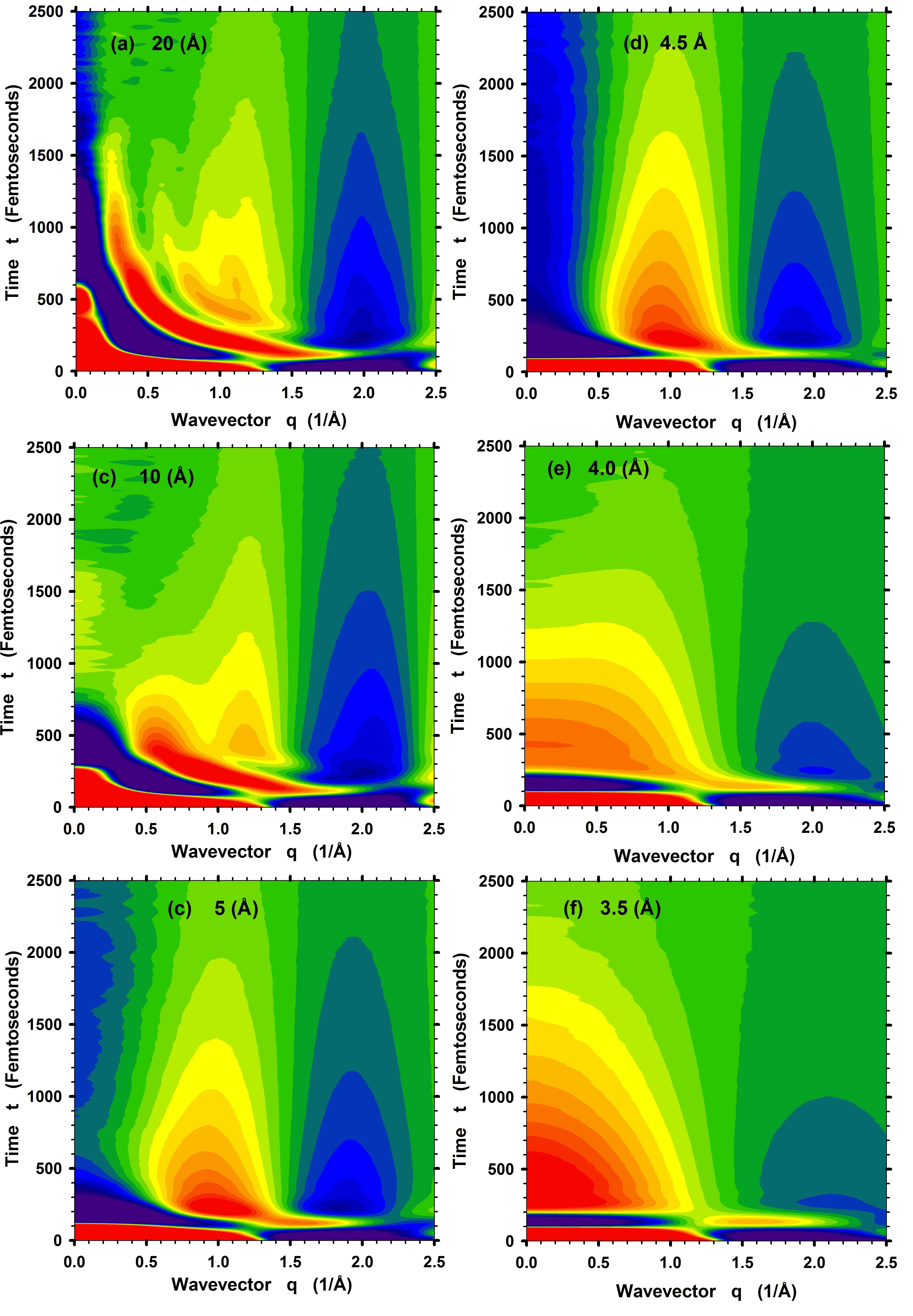
In order to understand the bonfire  feature in panels (3,1) and (3,2) of Fig.1 we adopt an ad hoc approach. In particular, in performing the Fourier transforms, we integrate from $r=0$ (Å) up to some maximum value $R_{max}$ and check how the value of $R_{max}$ affects the Fourier image. The results are shown in Fig.14.

Panel (a) shows the results of the integration up to $r=20$ (Å). Note the similarities and differences between the intensity in panel (a) and the intensity in panel (3,2) of Fig.1. For panel (b) $R_{max}=10$ (Å). By comparing panels (a) and (b) note that the negative intensity region close to $q=0$ (Å^-1) present in panel (a) is gone in panel (b). Similarly gone is the part of the sickle  feature that apparently originates from the part of the shear stress wave that we do not count when we integrate up to $R_{max}=10$ (Å). However, the bonfire  feature is still there, even though it is affected in the transition from (b) to (c). In panel (c) the negative intensity region around $q=0$ (Å^-1) appears again. Thus, from the comparison of panels (a), (b) and (c) we conclude that the negative intensity close to $q=0$ (Å^-1 is related to the spatial extent of the sscf  . Further note that the bonfire  feature is still present in panels (c) and (d). The transition from panel (d) to panel (e) affects the bonfire  feature very significantly. It follows from panel (a) of Fig.7 in Ref.Levashov2013 that the region between 4 (Å) and 5 (Å) corresponds to the interval of distances in which the splitting of the second peak in the pair density function occurs. Overall, we conclude that the bonfire  feature is related to the absence of periodicity in the sscf  for $r<10$ (Å^-1). Comparison of panels (1,2) and (3,2) of Fig.1 also hints that this conclusion is correct. Thus, one may notice that the temporal extent of the bonfire  feature in (3,2) corresponds to the temporal extent of the bright vertical stripes in the region $r<10$ (Å). The last idea can also be tested on the sscfs  and their Fourier transforms at higher temperatures, as can be seen in Fig.11,13. Thus a comparison of panels (1,1) and (1,3) of Fig.11 shows that the bright stripe present in (1,1) at 5 (Å) is significantly less pronounced in panel (1,3). The comparison of the corresponding panels in Fig.13 shows that the bonfire  feature is present in (1,1), but nearly absent in (1,3).

Appendix C The tongue  feature

In order to understand the tongue  feature present in panels (3,1) and (3,2) of Fig.1 we again adopt an ad hoc approach. Thus we create several model sscfs  and, by comparing the Fourier transforms of these sscfs  , we demonstrate that the line shape of the tongue  feature is affected by the behavior of stress waves at distances at which the stress waves appear.

It is shown in Ref.Landau6 that in viscous liquids in spherically symmetric homogeneous cases the pressure profile far away from the origin is given approximately by:

$$p^{\prime}(r,\tau)=p^{\prime}_{o}\frac{\tau}{r^{5/2}}\exp\left[-\frac{\tau^{2}}{4ar}\right]\;\;,$$ (25)

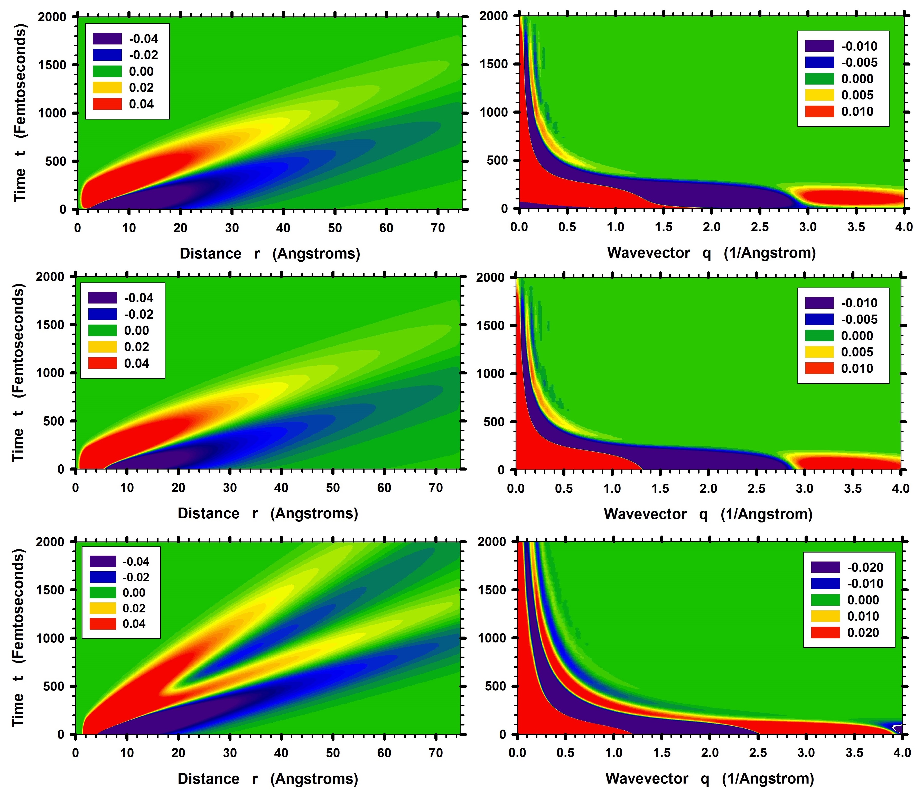
where $p^{\prime}(r,\tau)$ is the deviation of pressure from its average value in the system caused by the wave, $\tau\equiv t-r/c$, $c$ - is the speed of the wave, $r$ is the distance from the origin of the wave, and $a$ controls the rate of the dissipation of the wave. We use the functional form (25) to create several model sscfs  . This does not mean that we assume that (25) correctly describes the shape of the shear stress waves. However, we believe that this approach allows determination of the origin of the tongue  feature.

Panel (1,1) of Fig.15 shows the pressure profile calculated using (25) with the following values of the parameters: $c=30$ (Å/fs), $4a=2500$ (fs²/Å), and $p^{\prime}_{o}=1$. We use (25) to calculate the pressure profile for $r>2$ (Å). We assume that for smaller distances the pressure is zero. For smoothness we also convolute the function with the Gaussian function of width $\sigma_{r}=0.50$ (Å) along the $r$-axis and with width $\sigma_{t}=50$ (fs) along the $t$-axis.

Panel (1,2) shows the Fourier transform of panel (1,1) into $(t,q)$-space. We see in (1,2) the analogue of the tongue  feature and also the sickle  feature. Note, however, that close to the origin the tongue  feature has a negative intensity. We found that this negative intensity could be removed by assuming that the wave starts not at $r=0$ (Å), but instead at some finite distance. Thus, panel (2,1) of Fig.15 shows a pressure wave in which instead of $\tau\equiv t-r/c$ we used $\tau=t-(r-r_{b})/c$ with $r_{b}=3.3$ (Å). As before we assumed that for $r<2$ (Å) the pressure is zero and we convoluted the function with the parameters given above. Panel (2,2) shows the Fourier transform of (2,1) in $(t,q)$-space. Note that compared to panel (1,2) there is no negative intensity around the origin in panel (2,2). The comparison also could be made with panel (2,1) of Ref.Levashov20141 .

Panel (3,1) shows a pressure profile which is a sum of two waves. One wave is exactly the same as in panel (2,1). The second wave also starts at $3.3$ (Å) and has the following values of the parameters: $c=60$ (Å/fs), $4a=1000$ (fs²/Å) and $p^{\prime}_{o}=3$. We see in panel (3,2) that the second wave makes the sickle  feature much more pronounced. Note also the increased intensity and the increased width of the positive intensity region around $q=0$ (Å^-1).

Thus we conclude that the line shape of the tongue  feature results from the behavior of the stress waves near their origin.

References

- (1) J. P. Hansen and I. R. McDonald, Theory of Simple Liquids, 3rd ed. Academic Press, London, 2006, Chap. 8.
- (2) J.P. Boon and S. Yip, Molecular Hydrodynamics, Dover Publications Inc., New York, 1991.
- (3) D. J. Evans and G. P. Morriss, Non-Equilibrium Statistical Mechanics of Liquids, Cambridge University Press, Cambridge, 2008.
- (4) D. Levesque and L. Verlet, Phys. Rev. A, 7, 1690 (1973).
- (5) D. J. Evans, Phys. Rev. A 23, 2622, (1981)
- (6) W.E. Alley and B.J. Alder Phys. Rev. A 27, 3158, (1983)
- (7) W.E. Alley, B.J. Alder, and S. Yip, Phys. Rev. A. 27, 3174, (1983)
- (8) R.D. Mountain Phys. Rev. A 26, 2859, (1982)
- (9) B. J. Palmer, Phys. Rev. E 49, 359 (1994)
- (10) R. Zanghi, L.J. Kaufman, Phys. Rev. E 75, 051501 (2007)
- (11) R.M. Puscasu, B.D. Todd, P.J. Daivis, and J.S. Hansen, J. Chem. Phys. 133, 144907 (2010)
- (12) A. Furukawa, H. Tanaka, Phys. Rev. Lett. 103, 135703 (2009)
- (13) A. Furukawa, H. Tanaka, Phys. Rev. E 84, 061503 (2011)
- (14) A. Furukawa, Phys. Rev. E 87, 062321 (2013)
- (15) H. Mizuno and R. Yamamoto, Eur. Phys. J. E 35, 29 (2012)
- (16) H. Mizuno and R. Yamamoto, Phys. Rev. Lett. 110, 095901, (2013)
- (17) J. Kim, T. Keyes, J. Phys. Chem. B 109, 21445 (2005)
- (18) S. Tang, G.T. Evans, C.P. Mason, M.P. Allen, J. Chem. Phys. 102, 3794 (1995)
- (19) M.S. Green, J. Chem. Phys. 22, 398 (1954)
- (20) R. Kubo, J. Phys. Soc. Jpn. 12, 570 (1957)
- (21) E. Helfand, Phys. Rev. 119, 1, (1960)
- (22) C. Hoheisel and R. Vogelsang, Comp. Phys. Rep. 8, 1 (1988)
- (23) K. Meier, A. Laesecke, S. Kabelac, J. Chem. Phys. 121, i8, 3671 (2004)
- (24) A.A. Chialvo, P.T. Cummings, and D.J. Evans, Phys. Rev. E, 47, 1702 (1993).
- (25) M.P. Allen, D. Brown, and A.J. Masters, Phys. Rev. E, 49, 2488 (1994).
- (26) D. A. McQuarrie, Statistical Mechanics, Harper & Row, New York, 1976, Chap. 21. page 519 and problem number 21-60.
- (27) B.D. Todd and J.S. Hansen, Phys. Rev. E, 78, 051202 (2008).
- (28) B.D. Todd, J.S. Hansen, P.G. Daivis Phys. Rev. Lett, 100, 195901 (2008).
- (29) B. Kamgar-Parsi, E.G. D. Cohen, and I.M. de Schepper, Phys. Rev. A. 35, 4781 (1987)
- (30) I.M. de Schepper, E.G. D. Cohen, C. Bruin, J.C. van Rijs, W. Montfrooij, and A.A. de Graaf Phys. Rev. A. 38, 271 (1988)
- (31) I.M. Mryglod, I.P. Omelyan, Phys. Lett. A. 205, 401 (1995)
- (32) I.M. Mryglod, I.P. Omelyan, Mol. Phys. 90, 91 (1997)
- (33) I.M. Mryglod, I.P. Omelyan, Mol. Phys. 91, 1005 (1997)
- (34) I.M. Mryglod, I.P. Omelyan, Mol. Phys. 92, 913 (1997)
- (35) I.P. Omelyan, I.M. Mryglod, M.V. Tokarchuk, Condens. Matter Phys. 8, 41 (2005).
- (36) D. Bertolini, A. Tani, Phys. Rev. E 83, 031201 (2011).
- (37) V.A. Levashov, J.R. Morris, T. Egami, J. Chem. Phys. 138, 044507 (2013)
- (38) V.A. Levashov, J.R. Morris, T. Egami, Phys. Rev. Lett. 106, 115703, (2011).
- (39) G. Picard, A. Ajdari, F. Lequeux, and L. Bocquet, Eur. Phys. J. E, 15, 371 (2004).
- (40) V. Chikkadi, G. Wegdam, D. Bonn, B. Nienhuis, and P. Schall, Phys. Rev. Lett, 107, 198303 (2011).
- (41) J. Chattoraj and A. Lemaître, Phys. Rev. Lett, 111, 066001 (2013).
- (42) S. Mirigian and K.S. Schweizer, J. Chem. Phys. Lett, 4, 3648 (2013).
- (43) V.A. Levashov, ArXiv. 1403.6418v2, (2014)
- (44) N. Taraskin and S. R. Elliott, Physica B 316, 81 (2002)
- (45) H. Shintani, H. Tanaka, Nature Materials 7, 870, (2008)
- (46) A. Marruzzo, W. Schirmacher, A. Fratalocchi, and G. Ruocco Scientific Reports 3, 1407, (2013)
- (47) M. D. Ediger and P. Harrowell, J. Chem. Phys 137, 080901, (2012)
- (48) V.A. Levashov, T. Egami, R.S. Aga, J.R. Morris, Phys. Rev. E 78, 041202 (2008)
- (49) If the parameters of the Lennard-Jones (LJ) potential are chosen in such a way that the distance at which the LJ potential is zero is the same as the distance at which our potential is zero then (Å). Let us also assume that the depth of the LJ potential is the same as the depth of our potential, i.e., (eV). With this choice of parameters, the minimum of the LJ potential occurs at (Å), while the minimum of our potential is at (Å). If the radial density were the delta function located at , the corresponding first peaks in the structure function would occur (because of the spherical Fourier transform) at the first maximum of the function , i.e., at . Thus, (1/Å). The reduced value of the wavevector associated with this peak is . The characteristic time that follows from the chosen parameters of the LJ potential (assuming that is the mass of an iron atom) is: (fs). Thus, characteristic frequency is: (1/fs). The particle number density in our simulations, expressed in terms of the reduced density of the LJ potential, is: . Here, in particular, we report about simulations made at temperatures 1500 (K) and 2000 (K). These temperatures expressed in the reduced units, (), are: and . The triple point of the LJ potential at which simulations are often done Levesque19731 corresponds to and Meier20041 . The characteristic value of viscosity for the LJ potential is: (Pa s). The value of viscosity that we obtained in simulation with our potential at 1500 (K) is (Pa s), while at 2000 (K) it is (Pa s). In reduced units they are and . For comparison the reduced value of viscosity for the LJ liquid at the triple point is Meier20041 .
- (50) A. P. Sokolov, A. Kisliuk, M. Soltwisch, D. Quitmann, Phys. Rev. Lett. 69, 1540, (1992)
- (51) T. Tomida, T. Egami, Phys. Rev. B. 52, 3290, (1995)
- (52) T. Egami and D. Srolovitz, J. Phys. F: Met. Phys. 12, 2141 (1982).
- (53) S.P. Chen, T. Egami and V. Vitek, Phys. Rev. B 37, 2440 (1988)
- (54) V.A. Levashov, T. Egami, R.S. Aga, J.R. Morris, Phys. Rev. B 78, 064205 (2008)
- (55) T. Kustanovich, Y. Rabin, Z. Olami, Phys. Rev. B 67, 104206 (2003)
- (56) T. Kustanovich, Y. Rabin, Z. Olami, Physica. A 330, 271 (2003)
- (57) P. Hopkins, A. Fortini, A.J. Archer, and M. Schmidt, J. Chem. Phys., 133, 224505 (2010)
- (58) T. Keyes, J. Phys. Chem. A 101, 2921 (1997)
- (59) N. Taraskin and S. R. Elliott, Phys. Rev. B 61, 12017 (2000)
- (60) P. Tan, N. Xu, A.B. Schofield and L. Xu, Phys. Rev. Lett 108, 095501 (2012)
- (61) D.R. Bland, The Theory of Linear Viscoelasticity, Pergamon Press, Oxford (1960)
- (62) Z. Donkó, J. Goree, and P. Hartmann, Phys. Rev. E. 81, 056404, (2010)
- (63) C. Maggi, B. Jakobsen, T. Christensen, N. Boye, and J.C. Dyre, J. Phys. Chem. B 112, 16320, (2008)
- (64) Y. Feng, J. Goree, and B. Liu, Phys. Rev. E. 85, 066402, (2012)
- (65) See Fig.2 in Ref.Egami19821
- (66) B.E. Warren, X-ray Diffraction, Dover Publications, INC., New York (1990)
- (67) The lowest value of follows from the condition . Thus . For the system with (Å) we have (Å-1). For the system with (Å) we have (Å-1). Similarly, for the frequencies . If our data span time interval from to then we should not consider frequencies smaller than . For (fs) we have (fs-1).
- (68) Due to the several distinct regimes in the relaxation of the cross stress correlation functions we performed fittings for the large times only. The functional form of the fitting functions for the normalized cross stress correlation functions was: . At every temperature fitting curves were used at times larger than . The values of the parameters were chosen to obtain a reasonable agreement (from an eye perspective) between the simulation data and the fitting curves. These fittings are not systematic. The values of the parameters for different temperatures are: At (K): (fs), , (fs), , , (fs), . At (K): (fs), , (fs), , , (fs), . At (K): (fs), , (fs), , , (fs), . At (K): (fs), , (fs), , , (fs), . At (K): (fs), , (fs), , , (fs), . At (K): (fs), , (fs), , , (fs), .
- (69) T.M. Truskett, S. Torquato, S. Sastry, P.G. Debenedetti, F.H. Stillinger, Phys. Rev. E. 58, 3083, (1998)
- (70) A. Malins, J. Eggers, C.P. Royall, S.R. Williams, H. Tanaka, J. Chem. Phys. 138, 12A535, (2013)
- (71) S. Abraham, P. Harrowell, J. Chem. Phys. 137, 014506 (2012)
- (72) U. Buchenau, J. Chem. Phys. 134, 224501 (2011)
- (73) M.E. Cates, J.P. Wittmer, J.-P. Bouchaud, and P. Claudin Phys. Rev. Lett 81, 1841, (1998)
- (74) C.S. O Hern, S.A. Langer, A.J. Liu, and S.R. Nagel Phys. Rev. Lett 86, 111, (2001)
- (75) N. Lac̆ević and S.C. Glotzer, J. Phys. Chem. B 108, 19623 (2004)
- (76) D. Bi, J. Zhang, B. Chakraborty, R.P. Behringer, Nature 480, 355 (2011)
- (77) K.W. Desmond, P.J. Young, D. Chen and Eric R. Weeks, Soft Matter, 9, 3424 (2013)
- (78) C. Donati, J.F. Douglas, Walter Kob, S.J. Plimpton, P.H. Poole, and Sharon C. Glotzer, Phys. Rev. Lett 80, 2338, (1998)
- (79) Dynamical Heterogeneities in Glasses, Colloids and Granular Materials Edited by L. Berthier, G. Biroli, J.-P. Bouchaud, L. Cipelletti, and W. van Saarloos, Oxford University Press, 2011.
- (80) L. D. Landau and E. M. Lifshitz, Fluid Mechanics, 2nd ed. Reed Educational and Professional Publishing, London, 1987, Chap. 8.