Distributed, simple and stable network localization

Abstract

We propose a simple, stable and distributed algorithm which directly optimizes the nonconvex maximum likelihood criterion for sensor network localization, with no need to tune any free parameter. We reformulate the problem to obtain a gradient Lipschitz cost; by shifting to this cost function we enable a Majorization-Minimization (MM) approach based on quadratic upper bounds that decouple across nodes; the resulting algorithm happens to be distributed, with all nodes working in parallel. Our method inherits the MM stability: each communication cuts down the cost function. Numerical simulations indicate that the proposed approach tops the performance of the state of the art algorithm, both in accuracy and communication cost.

I Problem statement

The sensor network is represented as an undirected connected graph $\mathcal{G}=(\mathcal{V},\mathcal{E})$. The node set $\mathcal{V}=\{1,2,\dots,n\}$ denotes the sensors with unknown positions. There is an edge $i\sim j\in{\mathcal{E}}$ between sensors $i$ and $j$ if a noisy range measurement between nodes $i$ and $j$ is available at both, and if $i$ and $j$ can communicate with each other. The set of sensors with known positions, named anchors, is denoted by ${\mathcal{A}}=\{1,\ldots,m\}$. For each $i\in{\mathcal{V}}$, we let ${\mathcal{A}}_{i}\subset{\mathcal{A}}$ be the subset of anchors (if any) relative to which node $i$ also possesses a noisy range measurement.

Let ${\mathbb{R}}^{p}$ be the space of interest ($p=2$ for planar networks, and $p=3$ otherwise), $x_{i}\in{\mathbb{R}}^{p}$ the position of sensor $i$, and $d_{ij}$ the noisy range measurement between sensors $i$ and $j$, known by both $i$ and $j$. Without loss of generality, we assume $d_{ij}=d_{ji}$. Anchor positions are denoted by $a_{k}\in{\mathbb{R}}^{p}$. Similarly, $r_{ik}$ is the noisy range measurement between sensor $i$ and anchor $k$, available at sensor $i$.

The distributed network localization problem addressed in this work consists in estimating the sensors’ positions $x=\{x_{i}\,:\,i\in\mathcal{V}\}$, from the available measurements $\{d_{ij}\,:\,i\sim j\}\cup\{r_{ik}\,:\,i\in{\mathcal{V}},k\in{\mathcal{A}}_{i}\}$, through collaborative message passing between neighboring sensors in the communication graph ${\mathcal{G}}$.

Under the assumption of zero-mean, independent and identically-distributed, additive Gaussian measurement noise, the maximum likelihood estimator for the sensor positions is the solution of the optimization problem

$$\operatornamewithlimits{minimize}_{x}f(x),$$ (1)

where

$$f(x)=\sum_{i\sim j}\frac{1}{2}(\|x_{i}-x_{j}\|-d_{ij})^{2}+\sum_{i}\sum_{k\in\mathcal{A}_{i}}\frac{1}{2}(\|x_{i}-a_{k}\|-r_{ik})^{2}.$$

Problem (1) is nonconvex and difficult to solve. Even in the centralized setting (i.e., all measurements are available at a central node) currently available iterative techniques don’t claim convergence to the global optimum. Also, even with noiseless measurements, multiple solutions might exist due to ambiguities in the network topology itself[1].

Related work

The literature on sensor network localization can be divided on centralized and distributed approaches; the first category encompasses methods that use a central processing node, which collects all measurements and estimates the sensor positions. Distributed approaches require that each node computes its own position, working only with data collected locally and exchanged with neighbors. The body of work on centralized approaches to the problem is vast (e.g., [2, 3, 4, 5, 6]). At a smaller scale, distributed techniques based on convex relaxations of the problem are also abundant (for example, [7, 8, 9, 10, 11]) But distributed, and maximum likelihood (thus nonconvex) approaches to the sensor network localization problem are much less common. The algorithm presented in [12] is a nonlinear Gauss-Seidel approach: only one node works at a time and solves a source localization problem with neighbors playing the role of anchors. The nodes activate sequentially in a round-robin scheme. Thus, the time to complete just one cycle becomes proportional to the network size. Parallel algorithms — the ones we are interested in this paper — avoid altogether this issue, as all nodes operate simultaneously; moreover, adding or deleting a node raises no special synchronization concern. The work presented in [13] puts forward a two-stage algorithm which is parallel: in a first consensus phase, a Barzilai-Borwein (BB) step size is calculated, followed by a local gradient computation phase. It is known that BB steps do not necessarily decrease the objective function; as discussed in [14], an outer globalization scheme involving line searches is needed to ensure its stability. However, line searches are cumbersome to implement in a distributed setting and are, in fact, absent in [13]. Further, the algorithm requires the step size to be computed via consensus, and thus the number of consensus rounds needed is a parameter to tune. We will present an algorithm with simple implementation which is both parallel and stable, with no free parameters. We will compare experimentally the performance of our method with the distributed, parallel, state of the art method in [13] in Sec. V.

Contributions

We tackle directly the nonconvex problem in (1), with a simple and efficient algorithm which:

1. is parallel;

2. does not involve any free parameter definition;

3. is proven not to increase the value of the cost function at each iteration;

4. has better performance in positioning error and cost value than the state of the art method, while expending less in communications.

The first and second claims are addressed in Sec. IV, the third in Sec. III and the last one in Sec. V, dedicated to numerical experiments.

II Problem reformulation

We can reformulate Problem (1) as

$$\operatornamewithlimits{minimize}_{x_{i},y_{ij},w_{ik}} \sum_{i\sim j}\frac{1}{2}\|x_{i}-x_{j}-y_{ij}\|^{2}+$$ (2)

$$\sum_{i}\sum_{j\in{\cal A}_{i}}\frac{1}{2}\|x_{i}-a_{k}-w_{ik}\|^{2}$$

subject to $$\|y_{ij}\|=d_{ij},\;\|w_{ij}\|=r_{ij},$$

and rewrite (2) as

$$\operatornamewithlimits{minimize}_{x_{i},y_{ij},w_{ik}} \frac{1}{2}\|Ax-y\|^{2}+\sum_{i}\frac{1}{2}\|x_{i}\otimes 1-\alpha_{i}-w_{i}\|^{2}$$ (3)

subject to $$\|y_{ij}\|=d_{ij},\;\|w_{ik}\|=r_{ik},$$

with concatenated vectors $x=(x_{i})_{i\in\mathcal{V}}$, $y=(y_{ij})_{i\sim j}$, $\alpha_{i}=(a_{ik})_{k\in\mathcal{A}_{i}}$, and $w_{i}=(w_{ik})_{k\in\mathcal{A}_{i}}$. In (3), the symbol $1$ stands for the vector of ones. Matrix $A$ is the result of the Kronecker product of the arc-node incidence matrix $C$ with the identity matrix $I_{p}$: $A=C\otimes I_{p}$. Problem (3) is equivalent to

$$\operatornamewithlimits{minimize}_{x_{i},y_{ij},w_{ik}} \frac{1}{2}\left\|\begin{bmatrix}A&-I&0\end{bmatrix}\begin{bmatrix}x\\ y\\ w\end{bmatrix}\right\|^{2}+\frac{1}{2}\left\|Ex-\alpha-w\right\|^{2}$$

subject to $$\|y_{ij}\|=d_{ij},\;\|w_{ik}\|=r_{ik},$$

where $\alpha=(\alpha_{i})_{i\in\mathcal{V}}$, $w=(w_{i})_{i\in\mathcal{V}}$, and $E$ is a matrix with zeros and ones, selecting the entries in $\alpha$ and $w$ corresponding to each sensor node. We now collect all the optimization variables in $z=(x,y,w)$, and rewrite our problem as

$$\operatornamewithlimits{minimize}_{z} \frac{1}{2}\left\|\begin{bmatrix}A&-I&0\end{bmatrix}z\right\|^{2}+\frac{1}{2}\left\|\begin{bmatrix}E&0&-I\end{bmatrix}z-\alpha\right\|^{2}$$

subject to $$z\in\mathcal{Z},$$

where $\mathcal{Z}=\{z=(x,y,w):\|y_{ij}\|=d_{ij},i\sim j,w_{ik}=r_{ik},i\in\mathcal{V},k\in\mathcal{A}_{i}\}$. Problem (3) can be written as

$$\operatornamewithlimits{minimize}_{z} f(z)=\frac{1}{2}z^{T}Mz-b^{T}z$$ (4)

subject to $$z\in\mathcal{Z},$$ (5)

for $M$ and $b$ defined as

$$M = M_{1}+M_{2},$$  b = [ET0-I ]α, (6)

$$M_{1} = \begin{bmatrix}A^{T}\\ -I\\ 0\end{bmatrix}\begin{bmatrix}A&-I&0\end{bmatrix},$$  M_2 = [ET0-I ][E 0 -I ].

III Majorization-Minimization

To solve Problem (4) in a distributed way we must deal with the complicating off-diagonal entries of $M$ that couple the sensors’ variables. We emphasize a simple, but key fact:

Remark 1.

The function optimized in Problem (4) is quadratic in $z$ and, thus, has a Lipschitz continuous gradient [15], i.e.,

$$\|\nabla f(x)-\nabla f(y)\|\leq L\|x-y\|,$$

for some $L$ and all $x,y$.

From this property of function $f$ we can obtain the upper bound (also found in [15]) $f(z)\leq f(z^{t})+\left<\nabla f(z^{t}),z-z^{t}\right>+\frac{L}{2}\left\|z-z^{t}\right\|^{2}$, for any point $z^{t}$ and use it as a majorizer in the Majorization-Minimization framework[16]. This majorizer decouples the variables and allows for a distributed solution. Our algorithm is simply:

$$z^{t+1}=\operatornamewithlimits{argmin}_{z\in\mathcal{Z}}f(z^{t})+\left<\nabla f(z^{t}),z-z^{t}\right>+\frac{L}{2}\left\|z-z^{t}\right\|^{2}.$$ (7)

The solution of (7) is the projected gradient iteration [15]

$$z^{t+1}=\mathrm{P}_{\mathcal{Z}}\left(z^{t}-\frac{1}{L}\nabla f(z^{t})\right),$$ (8)

where $\mathrm{P}_{\mathcal{Z}}(p)$ is the projection of point $p$ onto $\mathcal{Z}$. The gradient in (8) can be easily computed as the affine function $\nabla f(z)=Mz-b.$ See the recent work [17] for interesting convergence properties of the recursion  (8). Particularly, we emphasize that the cost function is non increasing per iteration.

We now compute a Lipschitz constant $L$ for the gradient of the quadratic function in Problem (4), such that it is easy to estimate in a distributed way.

$$L = \lambda_{\mathrm{max}}\left(M\right)$$ (9)

$$\leq \lambda_{\mathrm{max}}\left(M_{1}\right)+\lambda_{\mathrm{max}}\left(M_{2}\right)$$

$$= \lambda_{\mathrm{max}}\left(AA^{T}+I\right)+\lambda_{\mathrm{max}}\left(EE^{T}+I\right)$$

$$\leq \lambda_{\mathrm{max}}\left(A^{T}A\right)+\lambda_{\mathrm{max}}\left(EE^{T}\right)+2$$

$$\leq 2\delta_{\mathrm{max}}+\max_{i\in\mathcal{V}}|\mathcal{A}_{i}|+2,$$

where $\lambda_{\mathrm{max}}$ denotes the largest eigenvalue, $|\mathcal{A}|$ is the cardinality of set $\mathcal{A}$, and $\delta_{\mathrm{max}}$ is the maximum node degree of the network. We note that $\lambda_{\mathrm{max}}(A^{T}A)$ is the maximum eigenvalue of graph $\mathcal{G}$ laplacian matrix; the proof that it is upper-bounded by $2\delta_{\mathrm{max}}$ can be found in [18]. This Lipschitz constant can be computed in a distributed way by, e.g., a diffusion algorithm (c.f. [19, Ch. 9]).

IV Distributed sensor network localization

At this point, the recursion in Eq. (8) is already distributed, as detailed below. From (8) we will obtain the update rules for the variables $x$, $y$ and $w$. For this we write matrix $M$ as follows:

$$M=\begin{bmatrix}A^{T}A+E^{T}E&-A^{T}&-E^{T}\\ -A&I&0\\ -E&0&I\end{bmatrix},$$ (10)

and denote $B=A^{T}A+E^{T}E$. Then, each block of $z$ is updated according to

Algorithm 1 Distributed nonconvex localization algorithm

0:  $x^{0};L;\{d_{ij}:j\in N_{i}\};\{r_{ik}:k\in\mathcal{A}_{i}\};$

0:  $\hat{x}$

1:  set $y_{ij}^{0}=\mathrm{P}_{\mathcal{Y}_{ij}}\left(x^{0}_{i}-x^{0}_{j}\right)$, $\mathcal{Y}_{ij}=\{y:\|y\|=d_{ij}\}$ and $w_{ik}^{0}=\mathrm{P}_{\mathcal{W}_{ik}}\left(x^{0}_{i}-a_{k}\right)$, $\mathcal{W}_{ik}=\{w:\|w\|=r_{ik}\}$

2:  $t=0$

3:  while some stopping criterion is not met, each node $i$ do

4:     $x_{i}^{t+1}=b_{i}x_{i}^{t}+\frac{1}{L}\sum_{j\in N_{i}}\left(x_{j}^{t}+C_{(i\sim j,i)}y_{ij}^{t}\right)+\frac{1}{L}\sum_{k\in\mathcal{A}_{i}}\left(w_{ik}^{t}+a_{ik}\right)$

5:     for all neighboring $j$, compute$y_{ij}^{k+1}=\mathrm{P}_{\mathcal{Y}_{ij}}\left(\frac{L-1}{L}y_{ij}^{k}+\frac{1}{L}C_{(i\sim j,i)}\left(x_{i}^{t}-x_{j}^{t}\right)\right),$

6:     for each of the connected anchors $k\in\mathcal{A}_{i}$, compute$w_{ik}^{t+1}=\mathrm{P}_{\mathcal{W}_{ik}}\left(\frac{L-1}{L}w_{ik}^{t}+\frac{1}{L}(x_{i}-a_{ik})\right)$

7:     broadcast $x_{i}^{t+1}$ to neighbors

8:     $t=t+1$

9:  end while

10:  return  $\hat{x}_{i}=x_{i}^{t}$

$$x^{t+1} = \left(I-\frac{1}{L}B\right)x^{t}+\frac{1}{L}A^{T}y^{t}+\frac{1}{L}E^{T}(w^{t}+\alpha),$$ (11)

$$y^{t+1} = \mathrm{P}_{\mathcal{Y}}\left(\frac{L-1}{L}y^{t}+\frac{1}{L}Ax^{t}\right),$$ (12)

$$w^{t+1} = \mathrm{P}_{\mathcal{W}}\left(\frac{L-1}{L}w^{t}+\frac{1}{L}Ex^{t}-\frac{\alpha}{L}\right),$$ (13)

where $\mathcal{Y}$ and $\mathcal{W}$ are the constraint sets associated with the acquired measurements between sensors, and between anchors and sensors, respectively, and $N_{i}$ is the set of the neighbors of node $i$. We observe that each block of $z=(x,y,w)$ at iteration $t+1$ will only need local neighborhood information, as clarified in Algorithm 1. Each node $i$ will update the current estimate of its own position, each one of the $y_{ij}$ for all the incident edges $i\sim j$ and the anchor terms $w_{ik}$, if any. The symbol $C_{(i\sim j,i)}$ denotes the arc-node incidence matrix entry relative to edge $i\sim j$ (row index) and node $i$ (column index). The constant $b_{i}$ in step 4 of Algorithm 1 is defined as $\frac{L-\delta_{i}-|\mathcal{A}_{i}|}{L}$.

V Experimental results

We present numerical experiments to ascertain the performance of the proposed Algorithm 1, both in accuracy and in communication cost. Accuracy will be measured in 1) mean positioning error per sensor, defined as

$$MPE=\frac{1}{n\cdot MC}\sum_{mc=1}^{MC}\sum_{i=1}^{n}\|\hat{x}_{i}(mc)-x_{i}^{\star}\|,$$ (14)

where $MC$ is the total number of Monte Carlo trials, $\hat{x}_{i}(mc)$ is the estimate generated by an algorithm at the Monte Carlo trial $mc$, and $x_{i}^{\star}$ is the true position of node $i$, and 2) also by evaluating the cost function in (1), averaged by the Monte Carlo trials and number of sensors, as in (14). Communication cost will be measured taking into account that each iteration in Algorithm 1 involves communicating $pn$ real numbers. We will compare the performance of the proposed method with the Barzilai-Borwein algorithm in [13], whose communication cost per iteration is $n(2T+p)$, where $T$ is the number of consensus rounds needed to estimate the Barzilai-Borwein step size. We use $T=20$ as in [13]. The setup for the experiments is a geometric network with $50$ sensors randomly distributed in the two-dimensional square $[0,\>1]\times[0,\>1]$, with average node degree of about $6$, and $4$ anchors placed at the vertexes of this square. The network remains fixed during all the Monte Carlo trials. Both algorithms receive an initialization from a convex approximation method. The initialization will hopefully hand the nonconvex refinement algorithms a point near the basin of attraction of the true minimum. For this purpose we generate noisy range measurements according to $d_{ij}=|\|x_{i}^{\star}-x_{j}^{\star}\|+\nu_{ij}|$, and $r_{ik}=|\|x_{i}^{\star}-a_{k}\|+\eta_{ik}|$, where  $\{\nu_{ij}:i\sim j\in\mathcal{E}\}\cup\{\eta_{ik}:i\in\mathcal{V},k\in\mathcal{A}_{i}\}$ are independent gaussian random variables with zero mean and standard deviation $\sigma$. We conducted $100$ Monte Carlo trials for each standard deviation $\sigma=(0.01,\>0.05,\>0.1)$. If we spread the sensors by a squared area with side of $1$Km, this means measurements are affected by noise of standard deviation of $10$m, $50$m, and $100$m.

TABLE I: Mean positioning error, with measurement noise

$\sigma$	Proposed method	BB method
0.01	0.0053	0.0059
0.05	0.0143	0.0154
0.10	0.0210	0.0221

In terms of mean positioning error per sensor the proposed algorithm fares better than the benchmark: Table I shows the mean error defined in (14) after the algorithms have stabilized, or reached a maximum iteration number. In a square with $1$Km sides, we improve the accuracy of the gradient descent with Barzilai-Borwein steps by about $1$m per sensor, even for high power noise.

(a) The proposed method improves the comparing algorithm, both in accuracy and communication cost. Our proposed method improves the state of the art method in [13] by about $60$ cm in mean positioning error per sensor, delivering a no surprises, stable progression of the error of the estimates.

(b) The final costs are, for the BB method, $1.7392\>10^{-4}$ and, for the proposed method $1.5698\>10^{-4}$. A small difference in cost that translates into a considerable distance in error, as depicted in Fig. 1(a) and Table I.

Figure 1: Noisy distance measurements with $\sigma=0.01$, representing $10$m for a square with $1$Km sides. The proposed method shows a faster and smoother progression, while the comparing method bounces, always above the proposed method.

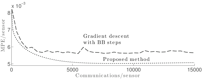
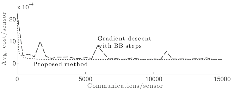
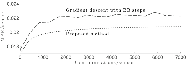
Fig. 1 depicts the averaged evolution of the error per sensor of both algorithms as a function of the volume of accumulated communications, and also the evolution of the cost. The gradient descent with Barzilai-Borwein steps shows an irregular pattern for the error, only vaguely matching the variation in the corresponding cost (Fig. 1(b)), thus leaving some uncertainty on when to stop the algorithm and what estimate to keep. The presented method reaches the final cost value per sensor much faster and steadily than the benchmark for medium-low measurement noise. In fact, our method takes under one order of magnitude less communications than the comparing one to approach the minimum cost value (match the cost at about $1500$ communications with $15000$).

(a) For medium noise power the algorithms’ performance comparison follows the one under low noise power. The accuracy gain is more than $1$m per sensor.

(b) Under medium noise the proposed method also reaches a smaller value for the average cost per sensor: $0.0031$, against $0.0032$ from the BB method.

Figure 2: Distance measurements contaminated with noise, with $\sigma=0.05$, representing $50$m for a square with $1$Km sides. The proposed method continues to outperform the comparing state of the art method, and contrasting the instability of the BB method.

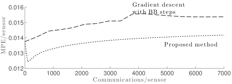
The most realistic case of medium noise power led to the results presented in Fig. 2. The characteristic irregularity of the BB method continues to fail in delivering better solutions in average than our stable, guaranteed method. The error curves in Fig. 2(a) are increasing, because the error is not the quantity being directly optimized and the medium-high noise power in measurement data shifts the cost optimal points.

(a) The proposed algorithm tops the comparing method in error, under high noise power, by more than $1$m, when considering a squared deployment area of $1$Km sides.

(b) Under heavy noise the proposed method reaches a smaller value for the average cost per sensor: $0.0096$, against $0.0099$ from the BB method.

Figure 3: Distance measurements contaminated with noise, with $\sigma=0.1$, representing $100$m for a square with $1$Km sides.

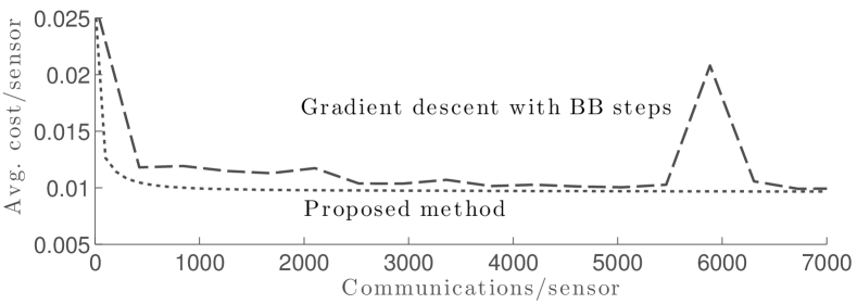
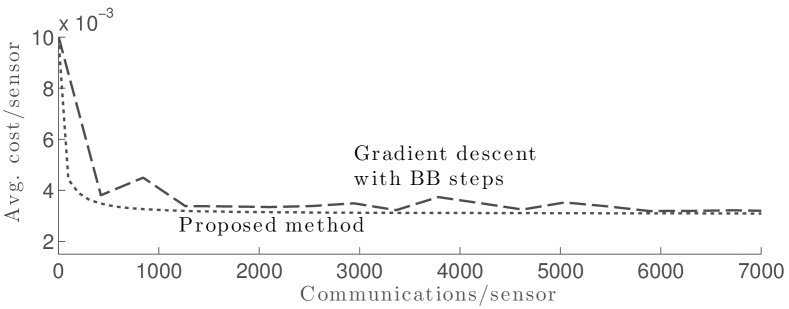
Under high noise power, our method tops the performance of the benchmark in cost function terms, as it is shown in Fig. 3(b), not only in the convergence speed, but also in the final value reached. Again, our method has almost one order of magnitude less in communications to achieve its plateau, which is itself, in average, better than the alternative method (compare the performance at $700$ communications with the one at $7000$).

VI Concluding remarks

The monotonicity of the proposed method is a strong feature for applications of sensor network localization. Our method proves to be not only fast and resilient, but also simple to implement and deploy, with no free parameters to tune. The steady accuracy gain over the competing method also makes it usable in contexts with a wide range of measurement errors are expected. The presented method can be useful both as a refinement algorithm and as a tracking method, e.g., for mobile robot formations where position estimates computed on a given time step are used as initialization for the next one.

References

- [1] B. D. O. Anderson, I. Shames, G. Mao, and B. Fidan, “Formal theory of noisy sensor network localization,” SIAM Journal on Discrete Mathematics, vol. 24, no. 2, pp. 684–698, 2010.
- [2] P. Oguz-Ekim, J. Gomes, J. Xavier, and P. Oliveira, “Robust localization of nodes and time-recursive tracking in sensor networks using noisy range measurements,” Signal Processing, IEEE Transactions on, vol. 59, no. 8, pp. 3930 –3942, aug. 2011.
- [3] G. Destino and G. Abreu, “On the maximum likelihood approach for source and network localization,” Signal Processing, IEEE Transactions on, vol. 59, no. 10, pp. 4954 –4970, oct. 2011.
- [4] P. Biswas, T.-C. Liang, K.-C. Toh, Y. Ye, and T.-C. Wang, “Semidefinite programming approaches for sensor network localization with noisy distance measurements,” Automation Science and Engineering, IEEE Transactions on, vol. 3, no. 4, pp. 360 –371, oct. 2006.
- [5] U. Khan, S. Kar, and J. Moura, “DILAND: An algorithm for distributed sensor localization with noisy distance measurements,” Signal Processing, IEEE Transactions on, vol. 58, no. 3, pp. 1940 –1947, mar. 2010.
- [6] D. Blatt and A. Hero, “Energy-based sensor network source localization via projection onto convex sets,” Signal Processing, IEEE Transactions on, vol. 54, no. 9, pp. 3614–3619, Sept 2006.
- [7] M. Gholami, L. Tetruashvili, E. Strom, and Y. Censor, “Cooperative wireless sensor network positioning via implicit convex feasibility,” Signal Processing, IEEE Transactions on, vol. 61, no. 23, pp. 5830–5840, Dec 2013.
- [8] A. Simonetto and G. Leus, “Distributed maximum likelihood sensor network localization,” Signal Processing, IEEE Transactions on, vol. 62, no. 6, pp. 1424–1437, March 2014.
- [9] Y. Keller and Y. Gur, “A diffusion approach to network localization,” Signal Processing, IEEE Transactions on, vol. 59, no. 6, pp. 2642 –2654, jun. 2011.
- [10] J. Costa, N. Patwari, and A. Hero III, “Distributed weighted-multidimensional scaling for node localization in sensor networks,” ACM Transactions on Sensor Networks (TOSN), vol. 2, no. 1, pp. 39–64, 2006.
- [11] S. Srirangarajan, A. Tewfik, and Z.-Q. Luo, “Distributed sensor network localization using SOCP relaxation,” Wireless Communications, IEEE Transactions on, vol. 7, no. 12, pp. 4886 –4895, dec. 2008.
- [12] Q. Shi, C. He, H. Chen, and L. Jiang, “Distributed wireless sensor network localization via sequential greedy optimization algorithm,” Signal Processing, IEEE Transactions on, vol. 58, no. 6, pp. 3328 –3340, jun. 2010.
- [13] G. Calafiore, L. Carlone, and M. Wei, “Distributed optimization techniques for range localization in networked systems,” in Decision and Control (CDC), 2010 49th IEEE Conference on, Dec 2010, pp. 2221–2226.
- [14] M. Raydan, “The barzilai and borwein gradient method for the large scale unconstrained minimization problem,” SIAM Journal on Optimization, vol. 7, no. 1, pp. 26–33, 1997.
- [15] D. P. Bertsekas, Nonlinear programming. Athena Scientific, 1999.
- [16] D. R. Hunter and K. Lange, “A tutorial on MM algorithms,” The American Statistician, vol. 58, no. 1, pp. 30–37, feb. 2004.
- [17] A. Beck and Y. Eldar, “Sparsity constrained nonlinear optimization: Optimality conditions and algorithms,” SIAM Journal on Optimization, vol. 23, no. 3, pp. 1480–1509, 2013. [Online]. Available: http://dx.doi.org/10.1137/120869778
- [18] F. R. Chung, Spectral graph theory. American Mathematical Soc., 1997, vol. 92.
- [19] M. Mesbahi and M. Egerstedt, Graph theoretic methods in multiagent networks. Princeton University Press, 2010.