Hanany-Witten effect and SL(2,)𝑆𝐿2SL(2,\mathbb{Z}) dualities
in matrix models


Benjamin Assel,
Abstract

We provide tests of dualities for three-dimensional 𝒩=4𝒩4\mathcal{N}=4 quiver SCFTs with brane realizations in IIB string theory, by matching their exact partition functions on S3superscript𝑆3S^{3}. The dualities are generated by SL(2,)𝑆𝐿2SL(2,\mathbb{Z}) transformations and Hanany-Witten 5-brane moves. These contain mirror symmetry as well as dualities identifiying fixed points of Yang-Mills quivers and Chern-Simons theories. The partition function is given by a matrix model, that can be nicely rearranged into a sequence of factors mimicking the brane realization. Identities obeyed by these elementary factors can be used to match the partition functions of dual theories, providing tests for the full web of dualities. In particular we are able to check mirror symmetry for linear and circular quivers with gauge nodes of arbitrary ranks. Our analysis also leads to a proof of a conjectured formula evaluating the matrix models of linear quiver SCFTs.

KCL-MTH-14-11

Department of Mathematics, King’s College London,

The Strand, London WC2R 2LS, United Kingdom

benjamin.assel@kcl.ac.uk


1 Introduction

𝒩=4𝒩4\mathcal{N}=4 Yang-Mills theories in three dimensions admit infrared strongly coupled fixed points, subject to the mirror symmetry duality [1]. Their moduli spaces split into a Coulomb branch and a Higgs branch that are exchanged under this duality. A prominent feature of these moduli spaces is that the Higgs branch does not receive quantum corrections and thus captures the quantum corrections to the Coulomb branch of the mirror theory. The 𝒩=4𝒩4\mathcal{N}=4 theories can be deformed by mass and Fayet-Iliopoulos terms, whose parameters are also exchanged under the duality. Mirror symmetry was extended to quiver theories in [2, 3], using the brane realizations of the theories in type IIB string theory [4]. The fixed point of a three-dimensional quiver theory was obtained as the low-energy theory of D3-branes suspended between NS5-branes and D5-branes. Mirror symmetry was then identified with the action of S-duality in IIB string theory, exchanging NS5-branes and D5-branes.

In [5] it was shown that the partition function of three-dimensional SCFTs deformed by mass and FI terms and defined on the round 3-sphere S3superscript𝑆3S^{3} can be computed exactly using localization techniques (see [6] for a review) and reduces to a simple matrix model. The exact partition function on S3superscript𝑆3S^{3} was then used in [7] to test mirror symmetry for IR fixed points of 𝒩=4𝒩4\mathcal{N}=4 circular Yang-Mills quiver theories with nodes of equal rank.

More tests of mirror symmetry by matching exact partition functions were given in [8, 9, 10] for A- and D-type quiver SCFTs. Other remarkable tests have been performed in [11, 12, 13, 14, 15], where the Hibert series of the Coulomb branch were shown to coincide with the Hilbert series of the Higgs branch of the mirror dual theories. Several cases were investigated there, involving mirror symmetry for A, D quivers and various star-shaped quivers. One of the interesting ideas developed in [15] is the possibility to generate new mirror pairs from the known dualities by gauging global symmetries.

Despite the significant advancements in testing mirror symmetry, very few results are known for the cases of quiver theories with nodes of different ranks. This gave the initial motivation for the present work, whose first ambition was to complete the tests of mirror symmetry for quiver theories with nodes of arbitrary ranks. The second idea was to understand the full SL(2,)𝑆𝐿2SL(2,\mathbb{Z}) duality group of the three-dimensional quiver theories, inherited from type IIB string theory [16]. It was shown in [17] that these more general dualities can map Yang-Mills fixed points to Chern-Simons theories coupled to matter. These are very interesting dualities since the Chern-Simons theories are superconformal, so that they would be indeed the infrared fixed point of the “dual” Yang-Mills theories. Three-dimensional Chern-Simons couplings have a priori only up to 𝒩=3𝒩3\mathcal{N}=3 supersymmetry, however with specific matter content and superpotentials the amount of supersymmetry can be enhanced to 𝒩=4𝒩4\mathcal{N}=4 [18, 19, 20], and up to 𝒩=8𝒩8\mathcal{N}=8 [21, 22].

In this paper we investigate these dualities by comparing the exact partition functions on S3superscript𝑆3S^{3} of the 𝒩=4𝒩4\mathcal{N}=4 Yang-Mills and Chern-Simons SCFTs deformed by mass and FI parameters, for linear and circular quivers with unitary nodes of arbitrary ranks. All the theories we consider admit brane realizations in IIB string theory as arrays of D3-branes suspended between two types of 5-branes. Yang-Mills quivers are realizated with NS5 and D5-branes; Chern-Simons quivers are realized with NS5 and (1,k)1𝑘(1,k)-5branes. Other choices of 5-branes lead to theories that were described in [23] as Chern-Simons theories with “interpolating T(U(N))𝑇𝑈𝑁T(U(N))” couplings. A web of dualities is generated by SL(2,)𝑆𝐿2SL(2,\mathbb{Z}) actions combined with Hanany-Witten 5-brane moves (HW moves). The HW moves exchange two 5-branes of different type in the sequence of 5-branes realizing a quiver theory. Mirror symmetry corresponds to the action of S𝑆S-duality combined with HW moves transforming the brane realization of a quiver theory into the brane realization of its mirror-dual. Other interesting dualities are generated, one being a level-rank duality for 𝒩=4𝒩4\mathcal{N}=4 Chern-Simons theories, corresponding to HW moves exchanging NS5 and (1,k)1𝑘(1,k)-5branes. Another duality relates Yang-Mills quivers to Chern-Simons quivers with Chern-Simons levels at each node being ±1plus-or-minus1\pm 1 or 00. A node with vanishing Chern-Simons level has an “auxiliary vector multiplet” [18, 24]. A class of Yang-Mills fixed points admit Chern-Simons duals with non-vanishing levels at all nodes, which correspond to microscopic descriptions of the infrared fixed point. Each mass or FI deformation parameter is associated to a the position of a 5-brane in the brane realization and the map between parameters is obtained by following the 5-branes through the duality transformations.

To test these dualities we decompose the matrix model which computes the partition function into a sequence of elementary factors, that can be associated to the 5-branes in the brane realization. This approach was already developed in [25] for quiver with nodes of equal ranks and we generalize it to quivers of arbitrary ranks and including mass and FI deformation terms. We then provide an action of SL(2,)𝑆𝐿2SL(2,\mathbb{Z}) dualities on the 5-brane factors, based on the analysis of [23], again generalizing [25]. This action on the matrix factors can be understood as a local SL(2,)𝑆𝐿2SL(2,\mathbb{Z}) duality on the brane configuration, introducing duality walls, that are associated to their own factors in the matrix model. The SL(2,)𝑆𝐿2SL(2,\mathbb{Z}) action on the 5-brane factors is used to prove the equality of the partition functions of any pair of SL(2,)𝑆𝐿2SL(2,\mathbb{Z})-dual theories, in a straightforward way. In practice, only two of the SL(2,)𝑆𝐿2SL(2,\mathbb{Z}) dualities will be relevant for us: S𝑆S duality which is related to mirror symmetry and the duality changing Yang-Mills theories into Chern-Simons theories. To include HW move dualities, we prove an identity for products of two 5-brane factors, mimicking the HW 5-brane exchange. Combining the SL(2,)𝑆𝐿2SL(2,\mathbb{Z}) action and this HW move-identity we are able to match the partition functions of any pair of quiver SCFTs related by this web of dualities. In particular we match the exact partition function of mirror dual YM quiver SCFTs with nodes of arbitrary ranks, deformed by parameters.

The main technical challenge in our computations was to find a matrix factor for a D5-brane with different numbers of D3-branes ending on its left and right sides. We found that it must be defined in terms of an unusual distribution δ^^𝛿\hat{\delta}. Although they look very exotic, these distributions proved very useful to derive the HW move identity. As a by-product our analysis leads to a proof of the formula conjectured in [26] (NTY formula) evaluating the matrix models of arbitrary deformed YM linear quiver SCFTs.

The map between partition functions that we found is only exact up to phases that depends on the mass and FI parameters. We argue, following [27, 28], that these phases affect contact terms in global current correlation functions and are unphysical in the sense that they arise from different UV regularizations (they can be removed by local counter-terms).

One lesson we learned from our analysis is that there is a close link between the matrix models and the brane realizations of the theories, and that what happens on the brane side always has a counterpart on the matrix model side, so that the brane picture is (as usual) a powerful guide to understand the properties of the gauge theories.

We also point out that the AdS4𝐴𝑑subscript𝑆4AdS_{4} gravity duals of the 𝒩=4𝒩4\mathcal{N}=4 quiver SCFTs studied in this paper (at vanishing deformation parameters) where constructed in [29, 30] in type IIB ten-dimensional supergravity. The counterparts in supergravity of the dualities we study are standard SL(2,)𝑆𝐿2SL(2,\mathbb{Z}) transformations of the gravity backgrounds.

The rest of the paper is organized as follows. In section 2 we give a brief description of the 𝒩=4𝒩4\mathcal{N}=4 three-dimensional theories that admit brane realizations. In section 3 we introduce the matrix models computing the partition functions on S3superscript𝑆3S^{3}, we explain the decomposition into 5-brane factors, we derive the SL(2,)𝑆𝐿2SL(2,\mathbb{Z}) action on the factors and prove the equality of partition functions for SL(2,)𝑆𝐿2SL(2,\mathbb{Z}) dual theories. In section 4 we prove the equality of the partition functions of theories related by HW move duality. We emphasize the cases of mirror symmetry and Yang-Mills/Chern-Simons dualities. In section 5 we give a proof of the NTY formula. Section 6 contains our conclusions and perspectives for future work. We also included three appendices: appendix A provides more details about the δ^^𝛿\hat{\delta} distributions, appendix B gathers a few useful formulas and appendix C contains details of computations.

2 𝒩=4𝒩4\mathcal{N}=4 theories with brane realizations

In this section we describe the 𝒩=4𝒩4\mathcal{N}=4 quiver theories and their type IIB brane realizations. We explain how to summerize the brane configuration, and thus the content of the quiver theory, in a graph with two types of nodes (or dots) and various labels.


Three-dimensional 𝒩=4𝒩4\mathcal{N}=4 gauge theories contain an 𝒩=4𝒩4\mathcal{N}=4 vector multiplet transforming in the adjoint representation of a gauge group G𝐺G and hypermultiplets transforming in arbitrary representations R𝑅R of G𝐺G. The 𝒩=4𝒩4\mathcal{N}=4 vector multiplet is made out of an 𝒩=2𝒩2\mathcal{N}=2 vector multiplet V𝑉V (in superfield notations) whose bosonic fields are a vector field Aμsubscript𝐴𝜇A_{\mu}, a real scalar σ𝜎\sigma and a real auxiliary field D𝐷D, and a chiral multiplet ΦΦ\Phi containing a complex scalar ϕitalic-ϕ\phi and a complex auxiliary field F𝐹F. A hypermultiplet contains two chiral multiplets Q,Q~𝑄~𝑄Q,\widetilde{Q} transforming in conjugate representations R𝑅R and R¯¯𝑅\bar{R} of the gauge group. The R-symmetry group is SU(2)V×SU(2)H𝑆𝑈subscript2𝑉𝑆𝑈subscript2𝐻SU(2)_{V}\times SU(2)_{H}, with the real scalars in the vector multiplet forming a SU(2)V𝑆𝑈subscript2𝑉SU(2)_{V} triplet and the scalars in the hypermultiplet forming two SU(2)H𝑆𝑈subscript2𝐻SU(2)_{H} doublets. 𝒩=4𝒩4\mathcal{N}=4 Yang-Mills theories are naturally endowed with canonical vector- and hyper-multiplet actions, given in terms of 𝒩=2𝒩2\mathcal{N}=2 superfields by:

Svec𝒩=4subscriptsuperscript𝑆𝒩4vec\displaystyle S^{\mathcal{N}=4}_{\rm vec} =1gYM2d3xd2θd2θ¯Tr(14Σ2+ΦeVΦ)absent1superscriptsubscript𝑔𝑌𝑀2superscript𝑑3𝑥superscript𝑑2𝜃superscript𝑑2¯𝜃Tr14superscriptΣ2superscriptΦsuperscript𝑒𝑉Φ\displaystyle=\frac{1}{g_{YM}^{2}}\int d^{3}xd^{2}\theta d^{2}\bar{\theta}\ \textrm{Tr}\left(\frac{1}{4}\Sigma^{2}+\Phi^{\dagger}e^{V}\Phi\right) (2.1)
Shyper𝒩=4subscriptsuperscript𝑆𝒩4hyper\displaystyle S^{\mathcal{N}=4}_{\rm hyper} =d3xd2θd2θ¯(QeVQ+Q~eVQ~),absentsuperscript𝑑3𝑥superscript𝑑2𝜃superscript𝑑2¯𝜃superscript𝑄superscript𝑒𝑉𝑄~𝑄superscript𝑒𝑉superscript~𝑄\displaystyle=\int d^{3}xd^{2}\theta d^{2}\bar{\theta}\left(Q^{\dagger}e^{V}Q+\widetilde{Q}e^{-V}\widetilde{Q}^{\dagger}\right)\ , (2.2)

with Σ=D¯αDαVΣsuperscript¯𝐷𝛼subscript𝐷𝛼𝑉\Sigma=\bar{D}^{\alpha}D_{\alpha}V (linear multiplet). In addition there is a superpotential coupling the adjoint chiral ΦΦ\Phi and the matter chirals Qi,Q~isubscript𝑄𝑖subscript~𝑄𝑖Q_{i},\widetilde{Q}_{i} of the form:

Ssp=d3xd2θ(iQ~iΦQi)+c.c..formulae-sequencesubscript𝑆spsuperscript𝑑3𝑥superscript𝑑2𝜃subscript𝑖subscript~𝑄𝑖Φsubscript𝑄𝑖𝑐𝑐\displaystyle S_{\rm sp}=\int d^{3}xd^{2}\theta\left(\sum_{i}\widetilde{Q}_{i}\Phi Q_{i}\right)+c.c.\ . (2.3)

In 3d the Yang-Mills coupling is dimensionful, gYM2superscriptsubscript𝑔𝑌𝑀2g_{YM}^{2} has the dimension of a mass, implying that the UV limit is free, while the IR limit is strongly interacting. For this reason, the above microscopic Lagrangian description is reliable only at high energies.

The theories can be deformed by supersymmetric mass terms for the hypermultiplets, obtained by coupling Q,Q~𝑄~𝑄Q,\widetilde{Q} to a background abelian 𝒩=4𝒩4\mathcal{N}=4 vector multiplet (Vm,Φm)subscript𝑉𝑚subscriptΦ𝑚(V_{m},\Phi_{m}), with Vm=mθ¯θsubscript𝑉𝑚𝑚¯𝜃𝜃V_{m}=m\,\bar{\theta}\theta and Φm=ϕmθ¯θsubscriptΦ𝑚subscriptitalic-ϕ𝑚¯𝜃𝜃\Phi_{m}=\phi_{m}\bar{\theta}\theta. (m,(m,Re(ϕm)subscriptitalic-ϕ𝑚(\phi_{m}),Im(ϕm))(\phi_{m})) form a triplet under SU(2)V𝑆𝑈subscript2𝑉SU(2)_{V}.

Supersymmetric FI deformation terms can aslo be added through a BF coupling to a background abelian 𝒩=4𝒩4\mathcal{N}=4 twisted vector multiplet (Vη,Φη)subscript𝑉𝜂subscriptΦ𝜂(V_{\eta},\Phi_{\eta}):

Sηsubscript𝑆𝜂\displaystyle S_{\eta} =d3xd2θd2θ¯Tr(ΣVη+ΦΦη)absentsuperscript𝑑3𝑥superscript𝑑2𝜃superscript𝑑2¯𝜃TrΣsubscript𝑉𝜂ΦsubscriptΦ𝜂\displaystyle=\int d^{3}xd^{2}\theta d^{2}\bar{\theta}\ \textrm{Tr}\left(\Sigma V_{\eta}+\Phi\Phi_{\eta}\right) (2.4)

with Vη=ηθ¯θsubscript𝑉𝜂𝜂¯𝜃𝜃V_{\eta}=\eta\,\bar{\theta}\theta and Φη=ϕηθ¯θsubscriptΦ𝜂subscriptitalic-ϕ𝜂¯𝜃𝜃\Phi_{\eta}=\phi_{\eta}\bar{\theta}\theta. (η,(\eta,Re(ϕη)subscriptitalic-ϕ𝜂(\phi_{\eta}),Im(ϕη))(\phi_{\eta})) form a triplet under SU(2)H𝑆𝑈subscript2𝐻SU(2)_{H}.

In this paper we focus on 𝒩=4𝒩4\mathcal{N}=4 theories which can be engineered on type IIB brane configurations involving D3-branes stretched between two types of 5-branes. The SCFTs arise in the infrared limit and the superconformal algebra is OSp(4|4)𝑂𝑆𝑝conditional44OSp(4|4).


2.1 Yang-Mills quiver SCFTs

We consider infrared fixed points of three-dimensional 𝒩=4𝒩4\mathcal{N}=4 theories that admit a realization as the low-energy limit of brane configurations in type-IIB string theory [4]. The brane configuration realizing Yang-Mills quivers consists of an array of D3, D5 and NS5 branes oriented as shown in the table. The D3 branes span a finite interval along the x3superscript𝑥3x^{3} direction and terminate on the five-branes. In the low-energy limit the world-volume SCFT on the D3-branes is effectively three-dimensionnal.

0 1 2 3 4 5 6 7 8 9
D3 X X X X
D5 X X X X X X
NS5 X X X X X X
Table 1: Brane array for three-dimensional quiver gauge theories

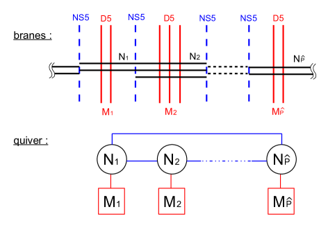
A stack of N𝑁N coincident D3-branes stretched between two NS5-branes and intersecting M𝑀M D5-branes give rise to a U(N)𝑈𝑁U(N) gauge group with Yang-Mills 𝒩=4𝒩4\mathcal{N}=4 vector multiplet, plus M𝑀M hypermultiplets in the fundamental representation of U(N)𝑈𝑁U(N). Moreover each NS5-brane introduces an additionnal hypermulitplet transforming in the bifundamental representation of U(Ni)×U(Ni+1)𝑈subscript𝑁𝑖𝑈subscript𝑁𝑖1U(N_{i})\times U(N_{i+1}), where Nisubscript𝑁𝑖N_{i} and Ni+1subscript𝑁𝑖1N_{i+1} are the numbers of D3-branes ending on the left and right of the NS5-brane respectively.

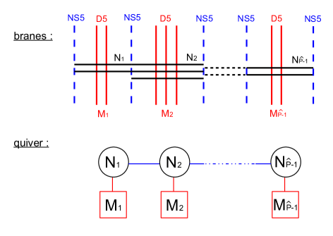
The brane configuration depicted in figure 1 is mapped to the linear quiver gauge theory summarized in the quiver diagram shown in the same figure. It contains P^^𝑃\hat{P} NS5-branes with Njsubscript𝑁𝑗N_{j} coincident D3-branes stretched between the j𝑗j-th and (j+1)𝑗1(j+1)-th NS5-brane and Mjsubscript𝑀𝑗M_{j} D5-branes intersecting the Njsubscript𝑁𝑗N_{j} D3-branes. In the quiver diagram a U(Nj)𝑈subscript𝑁𝑗U(N_{j}) gauge node, with Mjsubscript𝑀𝑗M_{j} fundamental hypermultiplets, is indicated by a circle with Njsubscript𝑁𝑗N_{j} and an attached square with Mjsubscript𝑀𝑗M_{j}. Bifundamental hypermultiplets are symbolized by lines joining two nodes. In total there are P^1^𝑃1\hat{P}-1 D3-segments (stacks of D3-branes), whose low energy dynamics is the same as the infrared fixed point of the quiver theory with P^1^𝑃1\hat{P}-1 gauge nodes. We also denote Pj=1P^1Mj𝑃superscriptsubscript𝑗1^𝑃1subscript𝑀𝑗P\equiv\sum_{j=1}^{\hat{P}-1}M_{j} the total number of D5-branes.

Refer to caption
Figure 1: Brane realization of linear quivers. Njsubscript𝑁𝑗N_{j} refers to the number of coincident D3-branes (parallel black lines) in a D3-segment and Mjsubscript𝑀𝑗M_{j} to the number of D5-branes crossing it. The horizontal direction can be thought as x3superscript𝑥3x^{3}. The vertical direction can be x456superscript𝑥456x^{456} for the D5s and x789superscript𝑥789x^{789} for the NS5s.

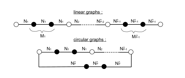
One can also compactify the x3superscript𝑥3x^{3} direction to a circle. The brane configuration is depicted in figure 2 and its low-energy theory corresponds to the low-energy limit of a circular quiver. The difference with respect to the linear quiver case is that the bifundamentals connecting the nodes form a closed loop.
Refer to caption
Figure 2: Brane realization of circular quivers. The D3-segments on the left and on the right are identified.

The deformations of the quiver SCFT by mass terms and FI terms can be associated to displacements of the 5-branes in transverse space. For instance we can take the convention that, if tjsubscript𝑡𝑗t_{j} denotes the position of the j𝑗jth NS5-brane along x9superscript𝑥9x^{9}, then the FI parameter of the j𝑗jth node is ηj=tjtj+1subscript𝜂𝑗subscript𝑡𝑗subscript𝑡𝑗1\eta_{j}=t_{j}-t_{j+1}, and if mjsubscript𝑚𝑗m_{j} denotes the position of the j𝑗jth D5-brane along x6superscript𝑥6x^{6}, then the corresponding hypermultiplet aquires a real mass mjsubscript𝑚𝑗m_{j}. Displacements of 5-branes along the other directions can be similarly mapped to the other FI and mass deformation parameters, but we will set them to zero in this work since they do not appear in the partition function on S3superscript𝑆3S^{3} computed by supersymmetric localization.


Graphs:


The brane pictures themselves can be recast into graphs, where a line labelled by N𝑁N denotes N𝑁N coincident D3-branes extended between two consecutive 5-branes, a white dot denotes a NS5-brane and a black dot denotes a D5-brane. This provides graphs associated to the the linear and circular quivers of figures 1, 2 as shown in figure 3.
Refer to caption
Figure 3: Graphs associated to linear and circular quivers.

2.1.1 T(U(N))𝑇𝑈𝑁T(U(N)) theory

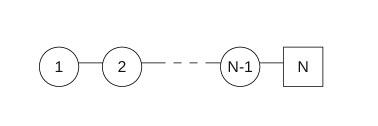
There is a Yang-Mills linear quiver SCFT that will play a distinguished role in our story: the T(U(N))𝑇𝑈𝑁T(U(N)) theory. Let us first described the theory T(SU(N))𝑇𝑆𝑈𝑁T(SU(N)). The UV quiver description has U(1)×U(2)××U(N1)𝑈1𝑈2𝑈𝑁1U(1)\times U(2)\times...\times U(N-1) gauge group, bifundamental hypermultiplets for each pair of adjacent nodes U(p)×U(p+1)𝑈𝑝𝑈𝑝1U(p)\times U(p+1), plus N𝑁N hypermultiplets in the fundamental representation of the U(N1)𝑈𝑁1U(N-1) node. T(SU(N))𝑇𝑆𝑈𝑁T(SU(N)) is the IR fixed point SCFT of this linear quiver (figure 4).
The theory has a group of global symmetry SU(N)F×SU(N)J𝑆𝑈subscript𝑁𝐹𝑆𝑈subscript𝑁𝐽SU(N)_{F}\times SU(N)_{J} with SU(N)F𝑆𝑈subscript𝑁𝐹SU(N)_{F} rotating the N𝑁N fundamental hypermultiplets and the SU(N)J𝑆𝑈subscript𝑁𝐽SU(N)_{J} arising as an enhancement of the topological U(1)N1𝑈superscript1𝑁1U(1)^{N-1} symmetry at the IR fixed point. The deformation parameters of T(SU(N))𝑇𝑆𝑈𝑁T(SU(N)), up to R-symmetry transformations, are N𝑁N real masses mjsubscript𝑚𝑗m_{j} for the N𝑁N fundamental hypermultiplets and N1𝑁1N-1 real FI parameters ηjsubscript𝜂𝑗\eta_{j} for the N1𝑁1N-1 nodes. T(SU(N))𝑇𝑆𝑈𝑁T(SU(N)) is known to be invariant under mirror symmetry, which exchanges the two SU(N)𝑆𝑈𝑁SU(N) global symmetries and the mass and FI parameters: ηjmjmj+1subscript𝜂𝑗subscript𝑚𝑗subscript𝑚𝑗1\eta_{j}\leftrightarrow m_{j}-m_{j+1}.

Refer to caption
Figure 4: T(SU(N))𝑇𝑆𝑈𝑁T(SU(N)) quiver diagram.

The diagonal U(1)F𝑈subscript1𝐹U(1)_{F} flavor symmetry, rotating the N𝑁N fundamental hypermultiplets by the same phase, is usually identified with the diagonal U(1)𝑈1U(1) of the gauge group. In the presence of generic supersymmetric FI deformations the diagonal U(1)𝑈1U(1) is coupled to a background twisted vector multiplet through a BF term and the flavor U(1)F𝑈subscript1𝐹U(1)_{F} may be considered formally as an independent symmetry, completing the flavor symmetry to U(N)F𝑈subscript𝑁𝐹U(N)_{F}.

To define the theory T(U(N))𝑇𝑈𝑁T(U(N)) we add an extra BF coupling between the background U(N)F𝑈subscript𝑁𝐹U(N)_{F} and a new background (twisted) abelian vector multiplet, defining a new symmetry that we call U(1)J𝑈subscript1𝐽U(1)_{J}. This is the same as adding a FI term for the U(N)F𝑈subscript𝑁𝐹U(N)_{F} flavor symmetry, with a FI parameter tNsubscript𝑡𝑁t_{N}. As we will see in section 3.1, the partition function of the T(U(N))𝑇𝑈𝑁T(U(N)) theory deformed by masses and FI terms is invariant under the exchange of the 2N2𝑁2N parameters mjtjsubscript𝑚𝑗subscript𝑡𝑗m_{j}\leftrightarrow t_{j}, with tjsubscript𝑡𝑗t_{j}, for 1jN11𝑗𝑁11\leq j\leq N-1 defined by ηj=tjtj+1subscript𝜂𝑗subscript𝑡𝑗subscript𝑡𝑗1\eta_{j}=t_{j}-t_{j+1}. It is then natural to combine the topological symmetry U(1)J𝑈subscript1𝐽U(1)_{J} with SU(N)J𝑆𝑈subscript𝑁𝐽SU(N)_{J} into a U(N)J𝑈subscript𝑁𝐽U(N)_{J} global symmetry.

A priori the T(U(N))𝑇𝑈𝑁T(U(N)) and T(SU(N))𝑇𝑆𝑈𝑁T(SU(N)) theories have identical dynamical properties, but it will be important for us to consider T(U(N))𝑇𝑈𝑁T(U(N)) to be able to gauge the U(N)F×U(N)J𝑈subscript𝑁𝐹𝑈subscript𝑁𝐽U(N)_{F}\times U(N)_{J} global symmetries.

To conclude we notice that the T(U(1))𝑇𝑈1T(U(1)) theory is rather trivial: it contains no dynamical field, but only a BF coupling between two abelian background vector multiplets.


2.2 Chern-Simons SCFTs


Three-dimensional gauge theories admit supersymmetric Chern-Simons terms, with quantized Chern-Simons level k𝑘k\in\mathbb{Z} 111In principle, depending on the number of massive chirals and their charges, the Chern-Simons level could be quantized to half-integer values [31]. However with the matter content of an 𝒩=4𝒩4\mathcal{N}=4 theory (only hypermultiplets), the quantization condition is simply k𝑘k\in\mathbb{Z}., preserving 𝒩=3𝒩3\mathcal{N}=3 sypersymmetry [32]. The action reads:

SCS𝒩=3subscriptsuperscript𝑆𝒩3CS\displaystyle S^{\mathcal{N}=3}_{\rm CS} =k4πd3xTr[ϵμνρ(AμνAρ+23AμAνAρ)+σDλ¯λ]k4πd3xd2θTr[Φ2+h.c.].\displaystyle=\frac{k}{4\pi}\int d^{3}x\ \textrm{Tr}\Big{[}\epsilon^{\mu\nu\rho}\left(A_{\mu}\partial_{\nu}A_{\rho}+\frac{2}{3}A_{\mu}A_{\nu}A_{\rho}\right)+\sigma D-\bar{\lambda}\lambda\Big{]}-\frac{k}{4\pi}\int d^{3}xd^{2}\theta\ \textrm{Tr}\Big{[}\Phi^{2}+h.c.\Big{]}\ . (2.5)

The Chern-Simons couping introduces a mass kgYM2similar-toabsent𝑘superscriptsubscript𝑔YM2\sim kg_{\rm YM}^{2} for the fields in the vector multiplet V𝑉V as well as for the adjoint chiral multiplet ΦΦ\Phi. In the infrared limit gYMsubscript𝑔𝑌𝑀g_{YM} becomes effectively very large, the Yang-Mills kinetic term is irrelevant and the adjoint chiral can be integrated out as an auxiliary field [32, 21], leading to a pure Chern-Simons theory with a new superpotential:

W𝑊\displaystyle W =4πk(iQ~iTRiaQi)(jQ~jTRjaQj),absent4𝜋𝑘subscript𝑖subscript~𝑄𝑖subscriptsuperscript𝑇𝑎subscript𝑅𝑖subscript𝑄𝑖subscript𝑗subscript~𝑄𝑗subscriptsuperscript𝑇𝑎subscript𝑅𝑗subscript𝑄𝑗\displaystyle=\frac{4\pi}{k}\left(\sum_{i}\widetilde{Q}_{i}\,T^{a}_{R_{i}}\,Q_{i}\right)\left(\sum_{j}\widetilde{Q}_{j}\,T^{a}_{R_{j}}\,Q_{j}\right)\ , (2.6)

with TRiasubscriptsuperscript𝑇𝑎subscript𝑅𝑖T^{a}_{R_{i}} the generators of the gauge group in the representation Risubscript𝑅𝑖R_{i}.

The 𝒩=3𝒩3\mathcal{N}=3 Chern-Simons theories are exactly conformal 222There is no relevant or marginal quantum correction to the classical action [32].. For specific choices of gauge group and matter content the Chern-Simons SCFTs can have enhanced 𝒩=4𝒩4\mathcal{N}=4 supersymmetry [18, 19, 20, 24], up to 𝒩=8𝒩8\mathcal{N}=8 supersymmetry corresponding to the ABJ(M) theory at Chern-Simons level k=1,2𝑘12k=1,2 (𝒩=6𝒩6\mathcal{N}=6 for k>2𝑘2k>2) [21, 22].

The brane realization of 𝒩=4𝒩4\mathcal{N}=4 Chern-Simons SCFTs described in [21] involves D3-branes, NS5-branes and (1,k)1𝑘(1,k)-5branes. The D3-branes are along the directions 012301230123, with the direction 333 compact, they intersect NS5-branes spanning 012789012789012789 and (1,k)1𝑘(1,k)-5branes spanning 012[4,7]θ[5,8]θ[6,9]θ012subscript47𝜃subscript58𝜃subscript69𝜃012[4,7]_{\theta}[5,8]_{\theta}[6,9]_{\theta}, with [a,b]θsubscript𝑎𝑏𝜃[a,b]_{\theta} meaning that the brane is along the direction cosθxa+sinθxb𝜃subscript𝑥𝑎𝜃subscript𝑥𝑏\cos\,\theta\,x_{a}+\sin\,\theta\,x_{b} in the (xa,xb)subscript𝑥𝑎subscript𝑥𝑏(x_{a},x_{b}) plane and the angle θ𝜃\theta is fixed as a function of k𝑘k so that the brane configuration preserves 𝒩=3𝒩3\mathcal{N}=3 supersymmetry [33], with a vanishing axion field. The low-energy theory living on the D3-branes has both Yang-Mills and Chern-Simons couplings. The Chern-Simons coupling for a U(N)𝑈𝑁U(N) node corresponding to N𝑁N D3-segments stretched between a (1,k1)1subscript𝑘1(1,k_{1})- and a (1,k2)1subscript𝑘2(1,k_{2})-5brane has CS level k1k2{k,0,k}subscript𝑘1subscript𝑘2𝑘0𝑘k_{1}-k_{2}\in\{-k,0,k\} [20, 34]. In the infrared limit, for nodes with non-zero Chern-Simons coupling ±kplus-or-minus𝑘\pm k, massive fields in the vector multiplet can be integrated out, as explained above, leading to a pure Chern-Simons node with a specific superpotential.

However, as mentioned in section 3.5 of [21], there exist alternative (or simpler) brane configurations realizing Chern-Simons-Matter SCFTs, that preserve 𝒩=4𝒩4\mathcal{N}=4 sypersymmetry. These are the same brane configurations as presented in section 2.1 with D5-branes replaced by (1,k)1𝑘(1,k)-5branes, namely the D3-branes are along 012301230123, the NS5-branes along 012789012789012789 and the (1,k)1𝑘(1,k)-5branes along 012456012456012456. This corresponds to the previous brane configurations with θ=π2𝜃𝜋2\theta=\frac{\pi}{2}, which preserves 𝒩=4𝒩4\mathcal{N}=4 (8 real supercharges) when allowing for non-vanishing axion field ([21]). For our purposes it makes more sense to consider these brane realizations that preserve the correct amount of supersymmetry and for which the SL(2,)𝑆𝐿2SL(2,\mathbb{Z}) action of type IIB string theory will be easily understood.

The theory living on D3-branes intersecting alternating NS5-branes and (1,k)1𝑘(1,k)-5branes involves U(N)𝑈𝑁U(N) Chern-Simons gauge nodes with alternating Chern-Simons levels ±kplus-or-minus𝑘\pm k and bifundamental hypermultiplets (twisted and untwisted alternatively) [19]. Moreover if the sequence of 5-branes have two consecutive NS5-branes or (1,k)1𝑘(1,k)-5branes, the infrared theory will have extra U(N)𝑈𝑁U(N) nodes without Chern-Simons term, nor Yang-Mills term, in which case the vector multiplet fields are auxiliary [18, 24]. Integrating out these auxiliary fields leads to a Chern-Simons gauge theory without these U(N)𝑈𝑁U(N) nodes, coupled to sigma models with hyper-Kähler target space [18].333For all we know, there is no difference between the infrared limit of a Yang-Mills node and an auxiliary node. The matrix models computing their partition functions are identical, so that we are not able to distinguish between the two cases.

For our purposes, it will be enough to describe the 𝒩=4𝒩4\mathcal{N}=4 infrared CFT living on a brane configuration associated to a sequence along x3superscript𝑥3x^{3} of NS5-branes and (1,k)1𝑘(1,k)-5branes as the infrared fixed point of a quiver theory with:

  • U(Ni)±k𝑈subscriptsubscript𝑁𝑖plus-or-minus𝑘U(N_{i})_{\pm k} Chern-Simons gauge node for Nisubscript𝑁𝑖N_{i} D3-segments extended between a NS5-brane and a (1,k)1𝑘(1,k)-5brane, with Chern-Simons level +k𝑘+k if the NS5-brane is on the left of the (1,k)1𝑘(1,k)-5brane along the x3superscript𝑥3x^{3} direction, and k𝑘-k otherwise.;

  • U(Ni)0𝑈subscriptsubscript𝑁𝑖0U(N_{i})_{0} auxiliary gauge node for Nisubscript𝑁𝑖N_{i} D3-branes stretched between two NS5-branes or two (1,k)1𝑘(1,k)-5branes, with 𝒩=4𝒩4\mathcal{N}=4 auxiliary vector multiplet ;

  • A bifundamental hypermultiplet (Xi,X~i)subscript𝑋𝑖subscript~𝑋𝑖(X_{i},\widetilde{X}_{i}) in (Ni,N¯i+1)(N¯i,Ni+1)direct-sumsubscript𝑁𝑖subscript¯𝑁𝑖1subscript¯𝑁𝑖subscript𝑁𝑖1(N_{i},\overline{N}_{i+1})\oplus(\overline{N}_{i},N_{i+1}) for each 5-brane with Nisubscript𝑁𝑖N_{i} D3-branes on its left and Ni+1subscript𝑁𝑖1N_{i+1} D3-branes on its right.

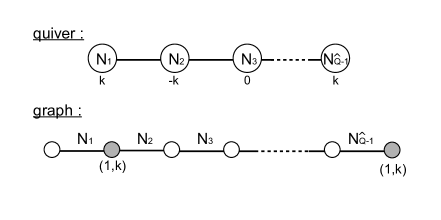
This is summarized in figure 5, where we also introduce the corresponding graph with white dots for NS5-branes and grey dots for (1,k)1𝑘(1,k)-5branes.
The superpotential for a U(Ni)k𝑈subscriptsubscript𝑁𝑖𝑘U(N_{i})_{k} Chern-Simons node is given by:

Wisubscript𝑊𝑖\displaystyle W_{i} =4πkTr(X~i1Xi1XiX~i).absent4𝜋𝑘Trsubscript~𝑋𝑖1subscript𝑋𝑖1subscript𝑋𝑖subscript~𝑋𝑖\displaystyle=\frac{4\pi}{k}\textrm{Tr}\left(\widetilde{X}_{i-1}X_{i-1}X_{i}\widetilde{X}_{i}\right)\ . (2.7)
Refer to caption
Figure 5: Chern-Simons quiver and its associated graph. The label below the nodes denotes the Chern-Simons level, zero meaning a node with auxiliary vector multiplet. The elements of the graph are white dots for NS5-branes and grey dots for (1,k)1𝑘(1,k)-5branes. Q𝑄Q is the total number of 5-branes, or dots, in the brane picture, or graph.

The Chern-Simons SCFTs admit deformations by FI terms associated to the positions of the 5-branes in transverse space, namely if tjsubscript𝑡𝑗t_{j} denotes the position of the j𝑗jth 5-brane along x9superscript𝑥9x^{9} (for NS5s) or x6superscript𝑥6x^{6} (for (1,k)1𝑘(1,k)5s), then the FI parameter of the j𝑗jth node is ηj=tjtj+1subscript𝜂𝑗subscript𝑡𝑗subscript𝑡𝑗1\eta_{j}=t_{j}-t_{j+1}.


2.3 SCFTs realized with (p,q)𝑝𝑞(p,q) 5-branes (GW quivers):


A natural extension of these brane constructions is to consider 𝒩=4𝒩4\mathcal{N}=4 SCFTs realized on brane configurations where D3-segments are stretched between (p1,q1)subscript𝑝1subscript𝑞1(p_{1},q_{1}) and (p2,q2)subscript𝑝2subscript𝑞2(p_{2},q_{2})-5branes oriented as the D5s and NS5s in table (1), with p1q1=1subscript𝑝1subscript𝑞11p_{1}\wedge q_{1}=1, p2q2=1subscript𝑝2subscript𝑞21p_{2}\wedge q_{2}=1 (coprime integers) and D=p1q2p2q10𝐷subscript𝑝1subscript𝑞2subscript𝑝2subscript𝑞10D=p_{1}q_{2}-p_{2}q_{1}\neq 0. Acting with the appropriate SL(2,)𝑆𝐿2SL(2,\mathbb{Z}) symmetry of type IIB string theory we can trade the (p1,q1)subscript𝑝1subscript𝑞1(p_{1},q_{1}) and (p2,q2)subscript𝑝2subscript𝑞2(p_{2},q_{2})-5-branes for NS5-branes and (p,q)𝑝𝑞(p,q)-5brane, with pq=1𝑝𝑞1p\wedge q=1 and q0𝑞0q\neq 0.

Even this simpler configurations with D3-segments stretched between NS5-branes and (p,q)𝑝𝑞(p,q)-5branes do not have a known Lagrangian description when p>1𝑝1p>1. It was argued in [23](section 8) using the SL(2,)𝑆𝐿2SL(2,\mathbb{Z}) symmetry of IIB string theory, that such theories have a dual description as the infrared fixed points of Chern-Simons quivers with T(U(N))𝑇𝑈𝑁T(U(N)) SCFTs “interpolating” between gauge nodes.

The precise gauge theory description demands to find the sequence of S𝑆S and T𝑇T transformations that brings the (p,q)𝑝𝑞(p,q)-5brane into a NS5-brane: (pq)=Tk1STk2SSTkr(10)binomial𝑝𝑞superscript𝑇subscript𝑘1𝑆superscript𝑇subscript𝑘2𝑆𝑆superscript𝑇subscript𝑘𝑟binomial10\binom{p}{q}=T^{k_{1}}ST^{k_{2}}S\cdots ST^{k_{r}}\binom{1}{0}, where S𝑆S and T𝑇T are the generators of the SL(2,)𝑆𝐿2SL(2,\mathbb{Z}) group (this will be reviewed in section 3.3). The relation between p,q𝑝𝑞p,q and the kisubscript𝑘𝑖k_{i} is

pq𝑝𝑞\displaystyle\frac{p}{q}\ =1k11k211kr.absent1subscript𝑘11subscript𝑘211subscript𝑘𝑟\displaystyle=\ \frac{1}{k_{1}-\frac{1}{k_{2}-\frac{1}{\cdots-\frac{1}{k_{r}}}}}\quad. (2.8)

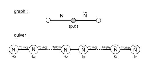
Then the SCFT corresponding to a sequence of 5-branes NS-(p,q)𝑝𝑞(p,q)-NS, with N𝑁N D3-branes in the first segment and N~~𝑁\widetilde{N} D3-branes in the second, can be described as the infrared fixed point of a Chern-Simons quiver theory with r1𝑟1r-1 “interpolating” T(U(N~))𝑇𝑈~𝑁T(U(\widetilde{N})) CFTs and r1𝑟1r-1 “interpolating” T(U(N))¯¯𝑇𝑈𝑁\overline{T(U(N))} as shown in figure 6. In this picture a link labelled with T(U(N))𝑇𝑈𝑁T(U(N)) denotes a coupling between a T(U(N))𝑇𝑈𝑁T(U(N)) SCFT and the two adjacent U(N)𝑈𝑁U(N) nodes by gauging the diagonal combination of the left U(N)L𝑈subscript𝑁𝐿U(N)_{L} node with the U(N)F𝑈subscript𝑁𝐹U(N)_{F} flavor symmetry of T(U(N))𝑇𝑈𝑁T(U(N)): U(N)L×U(N)FU(N)L𝑈subscript𝑁𝐿𝑈subscript𝑁𝐹𝑈subscript𝑁superscript𝐿U(N)_{L}\times U(N)_{F}\rightarrow U(N)_{L^{\prime}}, and gauging the diagonal combination of the right U(N)R𝑈subscript𝑁𝑅U(N)_{R} node with the U(N)J𝑈subscript𝑁𝐽U(N)_{J} “topological” symmetry of T(U(N))𝑇𝑈𝑁T(U(N)): U(N)R×U(N)JU(N)R𝑈subscript𝑁𝑅𝑈subscript𝑁𝐽𝑈subscript𝑁superscript𝑅U(N)_{R}\times U(N)_{J}\rightarrow U(N)_{R^{\prime}}. The coupling between T(U(N))𝑇𝑈𝑁T(U(N)) and the left node U(N)L𝑈subscript𝑁𝐿U(N)_{L} results in having a bifundamental hypermultiplet transforming in the (N1,N¯)(N1¯,N)direct-sum𝑁1¯𝑁¯𝑁1𝑁(N-1,\overline{N})\oplus(\overline{N-1},N) representation of U(N1)×U(N)L𝑈𝑁1𝑈subscript𝑁superscript𝐿U(N-1)\times U(N)_{L^{\prime}}, with U(N1)𝑈𝑁1U(N-1) the highest rank gauge node of T(U(N))𝑇𝑈𝑁T(U(N)), while the coupling between T(U(N))𝑇𝑈𝑁T(U(N)) and the right node U(N)R𝑈subscript𝑁𝑅U(N)_{R} does not have a known microscopic description.

A link labelled with T(U(N))¯¯𝑇𝑈𝑁\overline{T(U(N))} denotes a similar coupling between two adjacent U(N)𝑈𝑁U(N) gauge nodes of the quiver theory and the T(U(N))𝑇𝑈𝑁T(U(N)) SCFT by the diagonal gaugings U(N)L×[U(N)F]U(N)L𝑈subscript𝑁𝐿superscriptdelimited-[]𝑈subscript𝑁𝐹𝑈subscript𝑁superscript𝐿U(N)_{L}\times[U(N)_{F}]^{\dagger}\rightarrow U(N)_{L^{\prime}} 444The diagonal gauging U(N)L×U(N)FU(N)L𝑈subscript𝑁𝐿𝑈subscript𝑁𝐹𝑈subscript𝑁superscript𝐿U(N)_{L}\times U(N)_{F}\rightarrow U(N)_{L^{\prime}} means that we gauge the transformation acting with the same matrix MU(N)L𝑀𝑈subscript𝑁𝐿M\in U(N)_{L} and MU(N)F𝑀𝑈subscript𝑁𝐹M\in U(N)_{F}. The diagonal gauging U(N)L×[U(N)F]U(N)L𝑈subscript𝑁𝐿superscriptdelimited-[]𝑈subscript𝑁𝐹𝑈subscript𝑁superscript𝐿U(N)_{L}\times[U(N)_{F}]^{\dagger}\rightarrow U(N)_{L^{\prime}} means that we gauge the transformation acting with the matrix MU(N)L𝑀𝑈subscript𝑁𝐿M\in U(N)_{L} and MU(N)Fsuperscript𝑀𝑈subscript𝑁𝐹M^{\dagger}\in U(N)_{F}. and U(N)R×U(N)JU(N)R𝑈subscript𝑁𝑅𝑈subscript𝑁𝐽𝑈subscript𝑁superscript𝑅U(N)_{R}\times U(N)_{J}\rightarrow U(N)_{R^{\prime}}. This coupling between T(U(N))𝑇𝑈𝑁T(U(N)) and the left node U(N)L𝑈subscript𝑁𝐿U(N)_{L} results in having a bifundamental hypermultiplet that transforms in the (N1,N)(N1¯,N¯)direct-sum𝑁1𝑁¯𝑁1¯𝑁(N-1,N)\oplus(\overline{N-1},\overline{N}) representation of U(N1)×U(N)L𝑈𝑁1𝑈subscript𝑁superscript𝐿U(N-1)\times U(N)_{L^{\prime}}. 555In [23] the (subtle) difference between T(U(N))𝑇𝑈𝑁T(U(N)) and T(U(N))¯¯𝑇𝑈𝑁\overline{T(U(N))} couplings was ignored.

Refer to caption
Figure 6: Graph corresponding to a sequence NS-(p,q)𝑝𝑞(p,q)-NS of 5branes and the corresponding CS quiver theory with interpolating T(U(N~))𝑇𝑈~𝑁T(U(\widetilde{N})) and T(U(N))¯¯𝑇𝑈𝑁\overline{T(U(N))} couplings. The central link of the quiver is simply a bifundamental hypermultiplet.

A succession of n𝑛n (p,q)𝑝𝑞(p,q)-5branes between two NS5-branes is associated to the same quiver theory as in figure 6, except that the central bifundamental hypermultiplet of U(N)×U(N~)𝑈𝑁𝑈~𝑁U(N)\times U(\widetilde{N}) is replaced by a sequence of n𝑛n Yang-Mills nodes connected by bifundamental hypermultiplets.

We will refer to these SCFTs realized with (p,q)𝑝𝑞(p,q)-5branes as Gaiotto-Witten quiver theories (GW quivers). In general GW quiver theories do not admit a Lagrangian description, because of the interpolating T(U(N))𝑇𝑈𝑁T(U(N)) couplings, however this is not true for purely abelian theories. Abelian GW quivers involve interpolating T(U(1))𝑇𝑈1T(U(1)) and T(U(1))¯¯𝑇𝑈1\overline{T(U(1))}, that have a very simple Lagrangian description as BF couplings between adjacent U(1)𝑈1U(1) gauge nodes.

3 SL(2,)𝑆𝐿2SL(2,\mathbb{Z}) dualities

In this section we introduce the matrix model computing the partition function on S3superscript𝑆3S^{3}. We explain how to organize it into a sequence of 5-brane factors reproducing the sequence of the brane construction. Then we propose, following [25], an action of SL(2,)𝑆𝐿2SL(2,\mathbb{Z}) duality on the 5-brane factors and show the equality of partition functions of SL(2,)𝑆𝐿2SL(2,\mathbb{Z})-dual theories.

3.1 Partition function on S3superscript𝑆3S^{3}

In [5] it was shown that the partition function of three-dimensional SCFTs deformed by real mass and FI terms and defined on the round 3-sphere S3superscript𝑆3S^{3} can be computed exactly and reduces to a simple matrix model. We summarize here the building blocks of the partition function matrix model on S3superscript𝑆3S^{3} for 𝒩=4𝒩4\mathcal{N}=4 theories.


Through this paper we use the following short-hand notations

sh(x)=2sinh(πx),ch(x)=2cosh(πx),th(x)=tanh(πx)formulae-sequencesh𝑥2𝜋𝑥formulae-sequencech𝑥2𝜋𝑥th𝑥𝜋𝑥\displaystyle\textrm{sh}(x)=2\sinh(\pi x)\ ,\quad\textrm{ch}(x)=2\cosh(\pi x)\ ,\quad\textrm{th}(x)=\tanh(\pi x)
xij=xixj,jN=j=1N,j<kN=1j<kN,j,kN,M=j=1Nk=1M\displaystyle x_{ij}=x_{i}-x_{j}\ ,\quad\prod_{j}^{N}...=\prod_{j=1}^{N}...\quad,\quad\prod_{j<k}^{N}...=\prod_{1\leq j<k\leq N}...\quad,\quad\prod_{j,k}^{N,M}...=\prod_{j=1}^{N}\prod_{k=1}^{M}...

and similar notations for the sums ΣjN=Σj=1N,superscriptsubscriptΣ𝑗𝑁superscriptsubscriptΣ𝑗1𝑁\Sigma_{j}^{N}=\Sigma_{j=1}^{N},\cdots.

The localisation on S3superscript𝑆3S^{3} of the partition function ZS3subscript𝑍superscript𝑆3Z_{S^{3}} reduces the whole path integral to an integration over the Cartan subalgebra of the gauge group, divided by the order of the Weyl group |𝒲|𝒲|\mathcal{W}|. We give here explicit formulas for a U(N)𝑈𝑁U(N) gauge group.

ZS3subscript𝑍superscript𝑆3\displaystyle Z_{S^{3}} =1|𝒲|Cartan𝑑σZclassicZvectorZhyper=1N!jNdσjZclassicZvectorZhyper.absent1𝒲subscriptCartandifferential-d𝜎subscript𝑍classicsubscript𝑍vectorsubscript𝑍hyper1𝑁superscriptsubscriptproduct𝑗𝑁𝑑subscript𝜎𝑗subscript𝑍classicsubscript𝑍vectorsubscript𝑍hyper\displaystyle=\frac{1}{|\mathcal{W}|}\int_{\textrm{Cartan}}d\sigma\ Z_{\rm classic}\,Z_{\rm vector}\,Z_{\rm hyper}\ =\ \frac{1}{N!}\int\prod_{j}^{N}d\sigma_{j}\ Z_{\rm classic}\,Z_{\rm vector}\,Z_{\rm hyper}\ . (3.1)

The integrand receives contributions Zvector,Zhypersubscript𝑍vectorsubscript𝑍hyperZ_{\rm vector},Z_{\rm hyper} from the vector and hyper-multiplets of the theory, while Zclassicsubscript𝑍classicZ_{\rm classic} contains the contributions from Chern-Simons and FI terms. The σjsubscript𝜎𝑗\sigma_{j} are called eigenvalues. For a U(N)𝑈𝑁U(N) group, the σjsubscript𝜎𝑗\sigma_{j} are the diagonal components of the hermitians matrices in the algebra 𝔲(N)𝔲𝑁\mathfrak{u}(N). The 𝒩=4𝒩4\mathcal{N}=4 vector multiplet contributes a factor

Zvectorsubscript𝑍vector\displaystyle Z_{\rm vector} =detAdj(sh(σ))=i<jNsh(σij)2,forG=U(N).\displaystyle=\textrm{det}_{\rm Adj}\Big{(}\textrm{sh}(\sigma)\Big{)}\ =\ \prod_{i<j}^{N}\textrm{sh}(\sigma_{ij})^{2}\qquad,\ {\rm for}\ G=U(N)\ . (3.2)

A hypermultiplet in a representation R𝑅R of the gauge group with real mass m𝑚m 666It is meant that the two chiral multiplets transforming in R𝑅R and R¯¯𝑅\overline{R} have opposite real masses m𝑚-m and m𝑚m respectively. contributes a factor

Zhypersubscript𝑍hyper\displaystyle Z_{\rm hyper} =detR(1ch(σm))absentsubscriptdet𝑅1ch𝜎𝑚\displaystyle=\textrm{det}_{R}\left(\frac{1}{\textrm{ch}(\sigma-m)}\right)
=jN1ch(σjm),forRR¯=NN¯ofU(N)\displaystyle=\prod_{j}^{N}\frac{1}{\textrm{ch}(\sigma_{j}-m)}\qquad,\ {\rm for}\ R\oplus\overline{R}=N\oplus\overline{N}\ {\rm of}\ U(N) (3.3)
=i,jN,N~1ch(σiσ~jm),forRR¯=(N,N~¯)(N¯,N~)ofU(N)×U(N~).\displaystyle=\prod_{i,j}^{N,\widetilde{N}}\frac{1}{\textrm{ch}(\sigma_{i}-\widetilde{\sigma}_{j}-m)}\quad,\ {\rm for}\ R\oplus\overline{R}=(N,\overline{\widetilde{N}})\oplus(\overline{N},\widetilde{N})\ {\rm of}\ U(N)\times U(\widetilde{N})\ .

An 𝒩=3𝒩3\mathcal{N}=3 Chern-Simons term with level k𝑘k contributes a factor

ZCSsubscript𝑍CS\displaystyle Z_{\rm CS} =detF(eiπkσ2)=eiπkjNσj2.absentsubscriptdet𝐹superscript𝑒𝑖𝜋𝑘superscript𝜎2superscript𝑒𝑖𝜋𝑘superscriptsubscript𝑗𝑁superscriptsubscript𝜎𝑗2\displaystyle=\textrm{det}_{F}\Big{(}e^{i\pi k\sigma^{2}}\Big{)}\ =\ e^{i\pi k\sum_{j}^{N}\sigma_{j}^{2}}\ . (3.4)

A real Fayet-Iliopoulos term with parameter η𝜂\eta contributes a factor

ZFIsubscript𝑍FI\displaystyle Z_{\rm FI} =detF(e2iπησ)=e2iπηjNσj.absentsubscriptdet𝐹superscript𝑒2𝑖𝜋𝜂𝜎superscript𝑒2𝑖𝜋𝜂superscriptsubscript𝑗𝑁subscript𝜎𝑗\displaystyle=\textrm{det}_{F}\Big{(}e^{2i\pi\eta\sigma}\Big{)}\ =\ e^{2i\pi\eta\sum_{j}^{N}\sigma_{j}}\ . (3.5)

Here detRsubscript𝑅\det_{R} is the the determinant in the representation R𝑅R. The indices F𝐹F and AdjAdj{\rm Adj} refer to the fundamental and adjoint representations respectively.
Refer to caption
Figure 7: Some quiver theories.

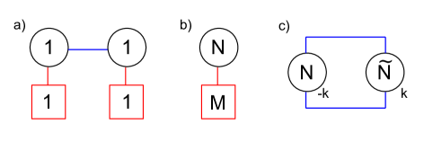
Let us give a few examples. The partition functions of the quiver SCFTs shown in figure 7 are given respectively by

Zasubscript𝑍𝑎\displaystyle Z_{a} =𝑑σ𝑑σ~e2πiησe2πiη~σ~ch(σm)ch(σσ~)ch(σ~m~)absentdifferential-d𝜎differential-d~𝜎superscript𝑒2𝜋𝑖𝜂𝜎superscript𝑒2𝜋𝑖~𝜂~𝜎ch𝜎𝑚ch𝜎~𝜎ch~𝜎~𝑚\displaystyle=\int d\sigma d\widetilde{\sigma}\ \frac{e^{2\pi i\eta\sigma}\ e^{2\pi i\widetilde{\eta}\widetilde{\sigma}}}{\textrm{ch}(\sigma-m)\,\textrm{ch}(\sigma-\widetilde{\sigma})\,\textrm{ch}(\widetilde{\sigma}-\widetilde{m})} (3.6)
Zbsubscript𝑍𝑏\displaystyle Z_{b} =dNσN!e2πiηjNσji<jNsh(σij)2a,jM,Nch(σjma)absentsuperscript𝑑𝑁𝜎𝑁superscript𝑒2𝜋𝑖𝜂superscriptsubscript𝑗𝑁subscript𝜎𝑗superscriptsubscriptproduct𝑖𝑗𝑁shsuperscriptsubscript𝜎𝑖𝑗2superscriptsubscriptproduct𝑎𝑗𝑀𝑁chsubscript𝜎𝑗subscript𝑚𝑎\displaystyle=\int\frac{d^{N}\sigma}{N!}\ e^{2\pi i\eta\sum_{j}^{N}\sigma_{j}}\frac{\prod_{i<j}^{N}\textrm{sh}(\sigma_{ij})^{2}}{\prod_{a,j}^{M,N}\textrm{ch}(\sigma_{j}-m_{a})} (3.7)
Zcsubscript𝑍𝑐\displaystyle Z_{c} =dNσN!dN~σN~!eπikjNσj2eπikjN~σ~j2e2πiηjNσje2πiη~jN~σ~ji<jNsh(σij)2i<jN~sh(σ~ij)2[i,jN,N~ch(σiσ~j)]2,absentsuperscript𝑑𝑁𝜎𝑁superscript𝑑~𝑁𝜎~𝑁superscript𝑒𝜋𝑖𝑘superscriptsubscript𝑗𝑁superscriptsubscript𝜎𝑗2superscript𝑒𝜋𝑖𝑘superscriptsubscript𝑗~𝑁superscriptsubscript~𝜎𝑗2superscript𝑒2𝜋𝑖𝜂superscriptsubscript𝑗𝑁subscript𝜎𝑗superscript𝑒2𝜋𝑖~𝜂superscriptsubscript𝑗~𝑁subscript~𝜎𝑗superscriptsubscriptproduct𝑖𝑗𝑁shsuperscriptsubscript𝜎𝑖𝑗2superscriptsubscriptproduct𝑖𝑗~𝑁shsuperscriptsubscript~𝜎𝑖𝑗2superscriptdelimited-[]superscriptsubscriptproduct𝑖𝑗𝑁~𝑁chsubscript𝜎𝑖subscript~𝜎𝑗2\displaystyle=\int\frac{d^{N}\sigma}{N!}\frac{d^{\widetilde{N}}\sigma}{\widetilde{N}!}\ e^{-\pi ik\sum_{j}^{N}\sigma_{j}^{2}}\,e^{\pi ik\sum_{j}^{\widetilde{N}}\widetilde{\sigma}_{j}^{2}}\,e^{2\pi i\eta\sum_{j}^{N}\sigma_{j}}\,e^{2\pi i\widetilde{\eta}\sum_{j}^{\widetilde{N}}\widetilde{\sigma}_{j}}\frac{\prod_{i<j}^{N}\textrm{sh}(\sigma_{ij})^{2}\prod_{i<j}^{\widetilde{N}}\textrm{sh}(\widetilde{\sigma}_{ij})^{2}}{[\,\prod_{i,j}^{N,\widetilde{N}}\textrm{ch}(\sigma_{i}-\widetilde{\sigma}_{j})\,]^{2}}\ , (3.8)

where η,η~𝜂~𝜂\eta,\widetilde{\eta} are real FI parameters, m,m~,ma𝑚~𝑚subscript𝑚𝑎m,\widetilde{m},m_{a} are real mass parameters and k,k𝑘𝑘k,-k are Chern-Simons levels.

The partition function of the T(SU(N))𝑇𝑆𝑈𝑁T(SU(N)) theory with fundamental hypermultiplet masses masubscript𝑚𝑎m_{a} and FI parameters ηpsubscript𝜂𝑝\eta_{p} is given by

ZT(SU(N))subscript𝑍𝑇𝑆𝑈𝑁\displaystyle Z_{T(SU(N))} (3.9)
=p=1N1(dpσ(p)p!i<jpsh(σij(p))2)p=1N1e2πiηpjpσj(p)p=1N2i,jp,p+1ch[σi(p)σj(p+1)]1a,jN,N1ch[σj(N1)ma]absentsuperscriptsubscriptproduct𝑝1𝑁1superscript𝑑𝑝superscript𝜎𝑝𝑝superscriptsubscriptproduct𝑖𝑗𝑝shsuperscriptsubscriptsuperscript𝜎𝑝𝑖𝑗2superscriptsubscriptproduct𝑝1𝑁1superscript𝑒2𝜋𝑖subscript𝜂𝑝superscriptsubscript𝑗𝑝subscriptsuperscript𝜎𝑝𝑗superscriptsubscriptproduct𝑝1𝑁2superscriptsubscriptproduct𝑖𝑗𝑝𝑝1chdelimited-[]subscriptsuperscript𝜎𝑝𝑖subscriptsuperscript𝜎𝑝1𝑗1superscriptsubscriptproduct𝑎𝑗𝑁𝑁1chdelimited-[]subscriptsuperscript𝜎𝑁1𝑗subscript𝑚𝑎\displaystyle=\int\prod_{p=1}^{N-1}\left(\frac{d^{p}\sigma^{(p)}}{p!}\ \prod_{i<j}^{p}\textrm{sh}\left(\sigma^{(p)}_{ij}\right)^{2}\right)\frac{\prod_{p=1}^{N-1}e^{2\pi i\,\eta_{p}\sum_{j}^{p}\sigma^{(p)}_{j}}}{\prod_{p=1}^{N-2}\prod_{i,j}^{p,p+1}\textrm{ch}[\sigma^{(p)}_{i}-\sigma^{(p+1)}_{j}]}\ \frac{1}{\prod_{a,j}^{N,N-1}\textrm{ch}[\sigma^{(N-1)}_{j}-m_{a}]}

The partition function for the theory T(U(N))𝑇𝑈𝑁T(U(N)) is the same with the addition of a FI coupling for the flavor U(N)F𝑈subscript𝑁𝐹U(N)_{F} global symmetry (background BF term):

ZT(U(N))subscript𝑍𝑇𝑈𝑁\displaystyle Z_{T(U(N))} =e2πitNjNmjZT(SU(N)),absentsuperscript𝑒2𝜋𝑖subscript𝑡𝑁superscriptsubscript𝑗𝑁subscript𝑚𝑗subscript𝑍𝑇𝑆𝑈𝑁\displaystyle=e^{2\pi i\,t_{N}\sum_{j}^{N}m_{j}}\ Z_{T(SU(N))}\ , (3.10)

with tNsubscript𝑡𝑁t_{N} the FI parameter. The evaluation of this matrix model was carried out in [35, 26] and gives

ZT(U(N))superscript𝑍𝑇𝑈𝑁\displaystyle Z^{T(U(N))} =(i)N(N1)2w𝒮N(1)we2iπjNtjmw(j)j<kNsh(tjtk)sh(mjmk)absentsuperscript𝑖𝑁𝑁12subscript𝑤subscript𝒮𝑁superscript1𝑤superscript𝑒2𝑖𝜋superscriptsubscript𝑗𝑁subscript𝑡𝑗subscript𝑚𝑤𝑗superscriptsubscriptproduct𝑗𝑘𝑁shsubscript𝑡𝑗subscript𝑡𝑘shsubscript𝑚𝑗subscript𝑚𝑘\displaystyle=(-i)^{\frac{N(N-1)}{2}}\frac{\sum_{w\in\mathcal{S}_{N}}(-1)^{w}\,e^{2i\pi\sum_{j}^{N}t_{j}m_{w(j)}}}{\prod_{j<k}^{N}\textrm{sh}(t_{j}-t_{k})\textrm{sh}(m_{j}-m_{k})} (3.11)

with 𝒮Nsubscript𝒮𝑁\mathcal{S}_{N} the group of permutations of N𝑁N elements and the tjsubscript𝑡𝑗t_{j} defined by the relations ηj=tjtj+1subscript𝜂𝑗subscript𝑡𝑗subscript𝑡𝑗1\eta_{j}=t_{j}-t_{j+1}, 1jN11𝑗𝑁11\leq j\leq N-1. ZT(U(N))superscript𝑍𝑇𝑈𝑁Z^{T(U(N))} is invariant under the exchange of the mass and FI parameters mjtjsubscript𝑚𝑗subscript𝑡𝑗m_{j}\leftrightarrow t_{j}, as it is expected from mirror symmetry.

3.2 Repackaging of matrix models

The partition function’s matrix model of a given quiver theory can be recast into a sequence of elementary matrix factors of two types, that are naturally associated to the two types of 5branes entering into the brane realization of the quiver. This sequence of elementary matrix factors reproduces the sequence of 5-branes, or dots, of the brane realization, or graph. We will treat the cases Yang-Mills and Chern-Simons quivers that involve NS5, D5 and (1,k)1𝑘(1,k)-5branes. The (p,q)𝑝𝑞(p,q)-5branes matrix factors will appear later.


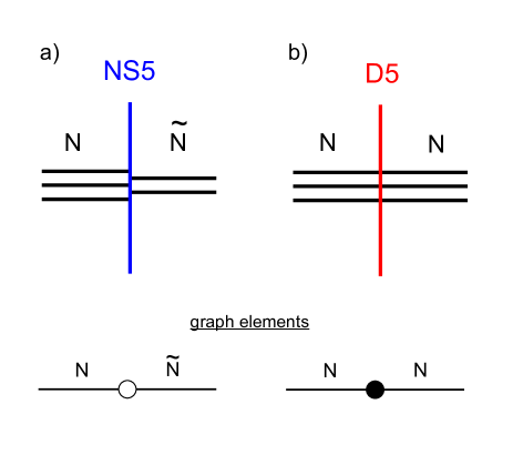
Let us start with Yang-Mills quivers. The brane realization and associated graph can be seen as a sequence made of two elementary 5-brane building blocks: one for the NS5-brane and one for the D5-brane as shown in figure 8.
Refer to caption
Figure 8: 5branes building blocks : a) NS5-brane. b) D5-brane. Below: corresponding graph elements in the graph description.

Each 5-brane block can be associated with a matrix factor depending on two sets on eigenvalues {σj,σ~j}subscript𝜎𝑗subscript~𝜎𝑗\{\sigma_{j},\widetilde{\sigma}_{j}\}, which are associated to the D3-branes ending on the left and on the right of the 5-brane respectively. The matrix model computing the partition function of the quiver theory is obtained by assembling the matrix factors of 5-branes blocks in a sequence reproducing the sequence of blocks of the brane realization, then identifying the eigenvalues of adjacent blocks (those corresponding to the same D3-segment) and finally integrating over all eigenvalues.

The NS5 matrix factor is given by

[10]σσ~subscriptdelimited-[]10𝜎~𝜎\displaystyle{\left[\begin{array}[]{c}1\\ 0\end{array}\right]}_{\sigma\,\widetilde{\sigma}} =1(N!N~!)1/2e2iπt(jNσj2jN~σ~j2)i<jNshσiji<jN~shσ~iji,jN,N~ch(σiσ~j).absent1superscript𝑁~𝑁12superscript𝑒2𝑖𝜋𝑡superscriptsubscript𝑗𝑁superscriptsubscript𝜎𝑗2superscriptsubscript𝑗~𝑁superscriptsubscript~𝜎𝑗2superscriptsubscriptproduct𝑖𝑗𝑁shsubscript𝜎𝑖𝑗superscriptsubscriptproduct𝑖𝑗~𝑁shsubscript~𝜎𝑖𝑗superscriptsubscriptproduct𝑖𝑗𝑁~𝑁chsubscript𝜎𝑖subscript~𝜎𝑗\displaystyle=\frac{1}{(N!\widetilde{N}!)^{1/2}}\,e^{-2i\pi\,t\left(\sum_{j}^{N}\sigma_{j}^{2}-\sum_{j}^{\widetilde{N}}\widetilde{\sigma}_{j}^{2}\right)}\frac{\prod_{i<j}^{N}\textrm{sh}\,\sigma_{ij}\ \prod_{i<j}^{\widetilde{N}}\textrm{sh}\,\widetilde{\sigma}_{ij}}{\prod_{i,j}^{N,\widetilde{N}}\textrm{ch}(\sigma_{i}-\widetilde{\sigma}_{j})}\ . (3.14)

It contains a bifundamental hypermultiplet matrix factor, “half” the matrix factors of the σ𝜎\sigma and σ~~𝜎\widetilde{\sigma} vector multiplets and “half” the matrix factors of the σ𝜎\sigma and σ~~𝜎\widetilde{\sigma} FI terms. In the brane picture t𝑡t is realted to the position of the NS5-brane in transverse space and it contributes to the FI terms of the two adjacent gauge nodes through the relations ηj=tjtj+1subscript𝜂𝑗subscript𝑡𝑗subscript𝑡𝑗1\eta_{j}=t_{j}-t_{j+1}, with ηjsubscript𝜂𝑗\eta_{j} the FI parameter of the j𝑗jth node and tjsubscript𝑡𝑗t_{j} the parameter of the j𝑗jth NS5-brane. The factor (N!N~!)1/2superscript𝑁~𝑁12(N!\widetilde{N}!)^{-1/2} are “half” the Weyl order of the left U(N)𝑈𝑁U(N) and right U(N~)𝑈~𝑁U(\widetilde{N}) groups.

The D5 matrix factor is given by

[01]σσ~subscriptdelimited-[]01𝜎~𝜎\displaystyle{\left[\begin{array}[]{c}0\\ 1\end{array}\right]}_{\sigma\,\widetilde{\sigma}} =1jNch(σjm)1N!w𝒮N(1)wjNδ(σjσ~w(j)),absent1superscriptsubscriptproduct𝑗𝑁chsubscript𝜎𝑗𝑚1𝑁subscript𝑤subscript𝒮𝑁superscript1𝑤superscriptsubscriptproduct𝑗𝑁𝛿subscript𝜎𝑗subscript~𝜎𝑤𝑗\displaystyle=\frac{1}{\prod_{j}^{N}\textrm{ch}(\sigma_{j}-m)}\ \frac{1}{N!}\sum_{w\in\mathcal{S}_{N}}(-1)^{w}\prod_{j}^{N}\delta(\sigma_{j}-\widetilde{\sigma}_{w(j)}), (3.17)

where 𝒮Nsubscript𝒮𝑁\mathcal{S}_{N} is the set of permutations of N𝑁N elements. The D5-factor contains the contribution of a fundamental hypermultiplet of mass m𝑚m. The σ𝜎\sigma and σ~~𝜎\widetilde{\sigma} eigenvalues are associated to the N𝑁N D3-segments ending on the left and on the right of the D5-brane and are identified, as they should, with the δ𝛿\delta functions. The averaging over permutations w𝒮N𝑤subscript𝒮𝑁w\in\mathcal{S}_{N} ensures the anti-symmetrization of the factor with respect to permutations of the σ𝜎\sigma or σ~~𝜎\widetilde{\sigma} eigenvalues, without affecting the matrix model. This anti-symmetrization will be naturally present in all 5-brane factors. In the brane picture m𝑚m is here again related to the position of the D5-brane in transverse space.


The (1,k)1𝑘(1,k)-5brane matrix factor is given by

[1k]σσ~subscriptdelimited-[]1𝑘𝜎~𝜎\displaystyle{\left[\begin{array}[]{c}1\\ k\end{array}\right]}_{\sigma\,\widetilde{\sigma}} =1(N!N~!)1/2e2iπt(jNσjjN~σ~j)eπik(jNσj2jN~σ~j2)i<jNshσiji<jN~shσ~iji,jN,N~ch(σiσ~j).absent1superscript𝑁~𝑁12superscript𝑒2𝑖𝜋𝑡superscriptsubscript𝑗𝑁subscript𝜎𝑗superscriptsubscript𝑗~𝑁subscript~𝜎𝑗superscript𝑒𝜋𝑖𝑘superscriptsubscript𝑗𝑁superscriptsubscript𝜎𝑗2superscriptsubscript𝑗~𝑁superscriptsubscript~𝜎𝑗2superscriptsubscriptproduct𝑖𝑗𝑁shsubscript𝜎𝑖𝑗superscriptsubscriptproduct𝑖𝑗~𝑁shsubscript~𝜎𝑖𝑗superscriptsubscriptproduct𝑖𝑗𝑁~𝑁chsubscript𝜎𝑖subscript~𝜎𝑗\displaystyle=\frac{1}{(N!\widetilde{N}!)^{1/2}}\,e^{-2i\pi\,t\left(\sum_{j}^{N}\sigma_{j}-\sum_{j}^{\widetilde{N}}\widetilde{\sigma}_{j}\right)}\ e^{\pi i\,k\left(\sum_{j}^{N}\sigma_{j}^{2}-\sum_{j}^{\widetilde{N}}\widetilde{\sigma}_{j}^{2}\right)}\ \frac{\prod_{i<j}^{N}\textrm{sh}\,\sigma_{ij}\ \prod_{i<j}^{\widetilde{N}}\textrm{sh}\,\widetilde{\sigma}_{ij}}{\prod_{i,j}^{N,\widetilde{N}}\textrm{ch}(\sigma_{i}-\widetilde{\sigma}_{j})}\ . (3.20)

In the brane picture t𝑡t is the position of the 5-brane in transverse space and it contributes to the FI terms of the left and right gauge nodes as in the NS5-brane case, which corresponds to k=0𝑘0k=0. As for the NS5-brane this factor contains the contribution of a bifundamental hypermultiplet and “half” the contributions of the vector multiplet of the two nodes on the sides of the (1,k)1𝑘(1,k)-5brane. Moreover this factor includes the contribution from the Chern-Simons term induced by the 5-brane, with levels ±kplus-or-minus𝑘\pm k in the two nodes.


To express conveniently matrix models, we define a “matrix-like” product:

([p1q1][p2q2](N))σσ~\displaystyle\left({\left[\begin{array}[]{c}p_{1}\\ q_{1}\end{array}\right]}{}_{(N)}{\left[\begin{array}[]{c}p_{2}\\ q_{2}\end{array}\right]}\right)_{\sigma\,\widetilde{\sigma}} =dNσ[p1q1]σσ[p2q2]σσ~.absentsuperscript𝑑𝑁superscript𝜎subscriptdelimited-[]subscript𝑝1subscript𝑞1𝜎superscript𝜎subscriptdelimited-[]subscript𝑝2subscript𝑞2superscript𝜎~𝜎\displaystyle=\int d^{N}\sigma^{\prime}\ {\left[\begin{array}[]{c}p_{1}\\ q_{1}\end{array}\right]}_{\sigma\,\sigma^{\prime}}{\left[\begin{array}[]{c}p_{2}\\ q_{2}\end{array}\right]}_{\sigma^{\prime}\,\widetilde{\sigma}}\ . (3.29)

This product 777We may sometimes use the even shorter notation [p1q1][p2q2]σσ~delimited-[]subscript𝑝1subscript𝑞1subscriptdelimited-[]subscript𝑝2subscript𝑞2𝜎~𝜎{\left[\begin{array}[]{c}p_{1}\\ q_{1}\end{array}\right]}{}{\left[\begin{array}[]{c}p_{2}\\ q_{2}\end{array}\right]}_{\sigma\,\widetilde{\sigma}}for such a product. is associative, but not commutative. Here (pi,qi)subscript𝑝𝑖subscript𝑞𝑖(p_{i},q_{i}) can be (0,1)01(0,1), (1,0)10(1,0) or (1,k)1𝑘(1,k), denoting a D5, NS5 or (1,k)1𝑘(1,k)-5brane factor. This “matrix-like” product will extend naturally to other matrix factors that we define later in section 3.3 (general (pi,qi)subscript𝑝𝑖subscript𝑞𝑖(p_{i},q_{i}) 5-brane factors and duality-wall factors). We also define a “trace” for a factor depending on two sets of N𝑁N eigenvalues Fσσ~subscript𝐹𝜎~𝜎F_{\sigma\,\widetilde{\sigma}} (“square matrix”):

TrF(N)Trsubscript𝐹𝑁\displaystyle\textrm{Tr}\,F_{(N)} =dNσFσσ.absentsuperscript𝑑𝑁𝜎subscript𝐹𝜎𝜎\displaystyle=\int d^{N}\sigma\ F_{\sigma\,\sigma}\ . (3.30)

This repackaging of the matrix model into elementary 5brane factors allows us to express the partition function’s matrix model in a compact way, as a sequence of 5brane factors. The partition function of a Yang-Mills linear quiver SCFT is expressed as888The sequence of factors here is just an example. In general it is given by its quiver data.

ZYMsubscript𝑍YM\displaystyle Z_{\rm YM} =[10][01](N1)[01](N1)[10](N1)[01](N2)[10](N2)(N3)[10](NP^1),\displaystyle={\left[\begin{array}[]{c}1\\ 0\end{array}\right]}{}_{(N_{1})}{\left[\begin{array}[]{c}0\\ 1\end{array}\right]}{}_{(N_{1})}{\left[\begin{array}[]{c}0\\ 1\end{array}\right]}{}_{(N_{1})}{\left[\begin{array}[]{c}1\\ 0\end{array}\right]}{}_{(N_{2})}{\left[\begin{array}[]{c}0\\ 1\end{array}\right]}{}_{(N_{2})}{\left[\begin{array}[]{c}1\\ 0\end{array}\right]}{}_{(N_{3})}\ \cdots\ {}_{(N_{\widehat{P}-1})}{\left[\begin{array}[]{c}1\\ 0\end{array}\right]}\ , (3.45)

where the first NS5-factor has no left-eigenvalues (no D3-segments on the left of the NS5-brane) and the last NS5-factor has no right-eigenvalues (no D3-segments on the right of the NS5-brane). The sequence of factors reproduces the sequence of NS5 and D5-branes of the quiver brane picture, or equivalently the sequence of white and black dots of the quiver’s graph, shown in figure 3.
For Yang-Mills circular quivers the partition function is expressed as

ZYMsubscript𝑍YM\displaystyle Z_{\rm YM} =Tr[10][01](N1)[01](N1)[10](N1)[01](N2)[10](N2)(N3)[10](NP^1).(NP^)\displaystyle=\textrm{Tr}\ {\left[\begin{array}[]{c}1\\ 0\end{array}\right]}{}_{(N_{1})}{\left[\begin{array}[]{c}0\\ 1\end{array}\right]}{}_{(N_{1})}{\left[\begin{array}[]{c}0\\ 1\end{array}\right]}{}_{(N_{1})}{\left[\begin{array}[]{c}1\\ 0\end{array}\right]}{}_{(N_{2})}{\left[\begin{array}[]{c}0\\ 1\end{array}\right]}{}_{(N_{2})}{\left[\begin{array}[]{c}1\\ 0\end{array}\right]}{}_{(N_{3})}\ \cdots\ {}_{(N_{\widehat{P}-1})}{\left[\begin{array}[]{c}1\\ 0\end{array}\right]}{}_{(N_{\widehat{P}})}\ . (3.60)

Again the sequence of factors reproduces the sequence of NS5 and D5-branes.
Let us give a few examples. The partition function of the T(SU(2))𝑇𝑆𝑈2T(SU(2)) theory is given by

ZT(SU(2))=[10][01](1)[01](1)[10](1),\displaystyle Z_{T(SU(2))}={\left[\begin{array}[]{c}1\\ 0\end{array}\right]}{}_{(1)}{\left[\begin{array}[]{c}0\\ 1\end{array}\right]}{}_{(1)}{\left[\begin{array}[]{c}0\\ 1\end{array}\right]}{}_{(1)}{\left[\begin{array}[]{c}1\\ 0\end{array}\right]}\ , (3.69)

the partition function of the U(2)𝑈2U(2) theory with four fundamental hypermultiplets is given by:

Z=[10][01](2)[01](2)[01](2)[01](2)[10](2),\displaystyle Z={\left[\begin{array}[]{c}1\\ 0\end{array}\right]}{}_{(2)}{\left[\begin{array}[]{c}0\\ 1\end{array}\right]}{}_{(2)}{\left[\begin{array}[]{c}0\\ 1\end{array}\right]}{}_{(2)}{\left[\begin{array}[]{c}0\\ 1\end{array}\right]}{}_{(2)}{\left[\begin{array}[]{c}0\\ 1\end{array}\right]}{}_{(2)}{\left[\begin{array}[]{c}1\\ 0\end{array}\right]}\ , (3.82)

and the partition function of the U(3)×U(4)𝑈3𝑈4U(3)\times U(4) circular quiver theory with two fundamental hypermultiplets for the U(4)𝑈4U(4) node is given by:

Z=Tr[10][01](4)[01](4)[10](4).(3)\displaystyle Z=\textrm{Tr}\ {\left[\begin{array}[]{c}1\\ 0\end{array}\right]}{}_{(4)}{\left[\begin{array}[]{c}0\\ 1\end{array}\right]}{}_{(4)}{\left[\begin{array}[]{c}0\\ 1\end{array}\right]}{}_{(4)}{\left[\begin{array}[]{c}1\\ 0\end{array}\right]}{}_{(3)}\ . (3.91)

The corresponding graphs are shown in figure 9.

Refer to caption
Figure 9: a) Graph of T(SU(2))𝑇𝑆𝑈2T(SU(2)). b) Graph of T(22)(1111)subscriptsuperscript𝑇111122T^{(1111)}_{(22)}. c) Graph of U(3)×U(4)𝑈3𝑈4U(3)\times U(4) circular quiver with two U(4)𝑈4U(4) fundamental hypermultiplets.

For Chern-Simons quivers, realized by a sequence of NS5-branes and (1,k)1𝑘(1,k)-5branes, the partition function is similarly expressed in the linear case by:

ZCSsubscript𝑍CS\displaystyle Z_{\rm CS} =[10][1k](N1)[1k](N1)[10](N1)[1k](N2)[10](N2)(N3)[10](NP^1),\displaystyle={\left[\begin{array}[]{c}1\\ 0\end{array}\right]}{}_{(N_{1})}{\left[\begin{array}[]{c}1\\ k\end{array}\right]}{}_{(N_{1})}{\left[\begin{array}[]{c}1\\ k\end{array}\right]}{}_{(N_{1})}{\left[\begin{array}[]{c}1\\ 0\end{array}\right]}{}_{(N_{2})}{\left[\begin{array}[]{c}1\\ k\end{array}\right]}{}_{(N_{2})}{\left[\begin{array}[]{c}1\\ 0\end{array}\right]}{}_{(N_{3})}\ \cdots\ {}_{(N_{\widehat{P}-1})}{\left[\begin{array}[]{c}1\\ 0\end{array}\right]}\ , (3.106)

and for circular quivers:

ZCSsubscript𝑍CS\displaystyle Z_{\rm CS} =Tr[10][1k](N1)[1k](N1)[10](N1)[1k](N2)[10](N2)(N3)[10](NP^1).(NP^)\displaystyle=\textrm{Tr}\ {\left[\begin{array}[]{c}1\\ 0\end{array}\right]}{}_{(N_{1})}{\left[\begin{array}[]{c}1\\ k\end{array}\right]}{}_{(N_{1})}{\left[\begin{array}[]{c}1\\ k\end{array}\right]}{}_{(N_{1})}{\left[\begin{array}[]{c}1\\ 0\end{array}\right]}{}_{(N_{2})}{\left[\begin{array}[]{c}1\\ k\end{array}\right]}{}_{(N_{2})}{\left[\begin{array}[]{c}1\\ 0\end{array}\right]}{}_{(N_{3})}\ \cdots\ {}_{(N_{\widehat{P}-1})}{\left[\begin{array}[]{c}1\\ 0\end{array}\right]}{}_{(N_{\widehat{P}})}\ . (3.121)

Again the sequence of 5brane blocks in Z𝑍Z reproduces the sequence of 5branes, or dots, in the brane realization, or graph.

For instance the partition function of the linear quiver U(1)k×U(1)0×U(1)k𝑈subscript1𝑘𝑈subscript10𝑈subscript1𝑘U(1)_{k}\times U(1)_{0}\times U(1)_{-k} is given by

Z=[10][1k](1)[1k](1)[10](1),\displaystyle Z={\left[\begin{array}[]{c}1\\ 0\end{array}\right]}{}_{(1)}{\left[\begin{array}[]{c}1\\ k\end{array}\right]}{}_{(1)}{\left[\begin{array}[]{c}1\\ k\end{array}\right]}{}_{(1)}{\left[\begin{array}[]{c}1\\ 0\end{array}\right]}\ , (3.130)

while the partition function of the circular quiver U(4)k×U(6)k×U(3)0𝑈subscript4𝑘𝑈subscript6𝑘𝑈subscript30U(4)_{k}\times U(6)_{-k}\times U(3)_{0} is given by

Z=Tr[10][1k](4)[10](6).(3)\displaystyle Z=\textrm{Tr}\ {\left[\begin{array}[]{c}1\\ 0\end{array}\right]}{}_{(4)}{\left[\begin{array}[]{c}1\\ k\end{array}\right]}{}_{(6)}{\left[\begin{array}[]{c}1\\ 0\end{array}\right]}{}_{(3)}\ . (3.137)

The corresponding graphs are shown in figure 10.

Refer to caption
Figure 10: a) Graph of U(1)k×U(1)0×U(1)k𝑈subscript1𝑘𝑈subscript10𝑈subscript1𝑘U(1)_{k}\times U(1)_{0}\times U(1)_{-k} linear CS quiver theory. b) Graph of U(4)k×U(6)k×U(3)0𝑈subscript4𝑘𝑈subscript6𝑘𝑈subscript30U(4)_{k}\times U(6)_{-k}\times U(3)_{0} circular CS quiver theory.

3.3 Local SL(2,\mathbb{Z}) action on matrix models

The quiver SCFTs realized on brane configurations must inherit SL(2,)𝑆𝐿2SL(2,\mathbb{Z}) dualities, from the SL(2,)𝑆𝐿2SL(2,\mathbb{Z}) symmetry of type IIB string theory. For instance the standard mirror symmetry, discussed in [1], is known to be related to the type IIB S𝑆S-duality.

In the case of standard mirror symmetry, dual pairs of quiver theories are found by identifying the brane realization of one theory with the S𝑆S-dual of the brane realization of the other theory [3, 2]. One theory is realized by a sequence of NS5 and D5-branes, while the mirror-dual theory is realized with the same sequence of 5branes, with NS5 and D5-branes exchanged (or NS5 \rightarrow D5, D5 NS5¯absent¯NS5\rightarrow\,\overline{\rm NS5}, see below).

More dualities can be found by identifying the brane realizations of quiver theories through general SL(2,)𝑆𝐿2SL(2,\mathbb{Z}) transformations of IIB string theory. We will give evidence for these more general dualities by matching the partition function of dual SCFTs. The dualities will actually extend to “local” SL(2,)𝑆𝐿2SL(2,\mathbb{Z}) dualities, that were already discussed in [25] and implicitly studied in [23].


Let us first remind and generalize the picture developed in [25] of SL(2,)𝑆𝐿2SL(2,\mathbb{Z}) action on the 5-brane factors of the matrix model.
The SL(2,)𝑆𝐿2SL(2,\mathbb{Z}) action on the brane realization of the 3d theories is easily understood. MSL(2,)𝑀𝑆𝐿2M\in SL(2,\mathbb{Z}) leaves the D3 branes invariant and transforms a (p,q)𝑝𝑞(p,q) 5brane into a (p,q)superscript𝑝superscript𝑞(p^{\prime},q^{\prime}) 5brane with

M𝑀\displaystyle M =(abcd),(pq)=M(pq)=(ap+bqcp+dq),formulae-sequenceabsent𝑎𝑏𝑐𝑑binomialsuperscript𝑝superscript𝑞𝑀binomial𝑝𝑞binomial𝑎𝑝𝑏𝑞𝑐𝑝𝑑𝑞\displaystyle={\left(\begin{array}[]{cc}a&b\\ c&d\end{array}\right)}\ ,\quad\binom{p^{\prime}}{q^{\prime}}=M\ \binom{p}{q}=\binom{ap+bq}{cp+dq}\ , (3.140)

where adbc=1𝑎𝑑𝑏𝑐1ad-bc=1 and pq=1𝑝𝑞1p\wedge q=1. The group SL(2,)𝑆𝐿2SL(2,\mathbb{Z}) is generated by the transformations S𝑆S and T𝑇T given by

S𝑆\displaystyle S =(0110),T=(1011),formulae-sequenceabsent0110𝑇1011\displaystyle={\left(\begin{array}[]{cc}0&-1\\ 1&0\end{array}\right)}\ ,\quad T={\left(\begin{array}[]{cc}1&0\\ 1&1\end{array}\right)}\ ,

satifying S2=1superscript𝑆21S^{2}=-1 and (ST)3=1superscript𝑆𝑇31(ST)^{3}=1.

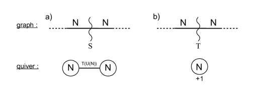
In [23] Gaiotto and Witten suggested that SL(2,)𝑆𝐿2SL(2,\mathbb{Z}) transformations can be realized locally on the brane configuration, in a region containing a single 5-brane (spanning an interval along x3superscript𝑥3x^{3} around the 5-brane). The authors of [25] reformulated their results in the following way. The local action of the transformation S𝑆S on a (p,q)𝑝𝑞(p,q)-5brane trades the (p,q)𝑝𝑞(p,q)-5brane for a (q,p)𝑞𝑝(-q,p)-5brane and creates an S𝑆S-duality wall on its right and a S1superscript𝑆1S^{-1} duality wall on its left (hyperplanes at fixed x3superscript𝑥3x^{3}). The duality walls are the boundaries of the region of local SL(2,)𝑆𝐿2SL(2,\mathbb{Z}) action and can be considered as new objects in the brane construction. From the analysis of [23] it follows that a S𝑆S-duality wall intersecting N𝑁N D3-branes induces in the quiver SCFT an interpolating T(U(N))𝑇𝑈𝑁T(U(N)) coupling between two U(N)𝑈𝑁U(N) gauge nodes (see sec. 2.3), that are associated to the D3-branes on the left and on the right of the S𝑆S-wall, as shown in figure 11. And the S1superscript𝑆1S^{-1}-wall intersecting N𝑁N D3-branes induces an interpolating T(U(N))¯¯𝑇𝑈𝑁\overline{T(U(N))} coupling between the two U(N)𝑈𝑁U(N) nodes.

Similarly the local action of T𝑇T on a (p,q)𝑝𝑞(p,q)-5brane trades the (p,q)𝑝𝑞(p,q)-5brane for a (p,p+q)𝑝𝑝𝑞(p,p+q)-5brane with a T𝑇T-duality wall on its right and a T1superscript𝑇1T^{-1}-duality wall on its left. From [23] it follows that a T𝑇T-duality wall intersecting N𝑁N D3-branes induces in the quiver SCFT a Chern-Simons term with level k=+1𝑘1k=+1 for a U(N)𝑈𝑁U(N) node, associated with the N𝑁N D3-branes crossing the T𝑇T-wall, as shown in figure 11. The T1superscript𝑇1T^{-1}-wall induces a Chern-Simons term with coupling k=1𝑘1k=-1.

The iterations of S𝑆S and T𝑇T local actions bringing a (p,q)𝑝𝑞(p,q)-5brane to a NS5-brane lead to the quiver theory description of SCFTs realized with (p,q)𝑝𝑞(p,q)-5branes, presented in section 2.3.

Refer to caption
Figure 11: Graph representations and quiver descriptions of the S𝑆S-duality wall (a) and T𝑇T-duality wall (b). The subscript +11+1 indices a Chern-Simons term at level k=1𝑘1k=1.

It is rather easy now to associate matrix factors to the S𝑆S- and T𝑇T-duality walls, as we did for the 5branes. The S𝑆S-wall with N𝑁N D3-branes on both sides must be associated to the contribution of an interpolating T(U(N))𝑇𝑈𝑁T(U(N)), plus “half” the contribution of the left and right U(N)𝑈𝑁U(N) vector multiplets and some phase eiθsuperscript𝑒𝑖𝜃e^{i\theta} to be fixed:

Sσσ~=eiθN!i<jNshσijZT(U(N))[σ,σ~]i<jNshσ~ijsubscript𝑆𝜎~𝜎superscript𝑒𝑖𝜃𝑁superscriptsubscriptproduct𝑖𝑗𝑁shsubscript𝜎𝑖𝑗subscript𝑍𝑇𝑈𝑁𝜎~𝜎superscriptsubscriptproduct𝑖𝑗𝑁shsubscript~𝜎𝑖𝑗\displaystyle S_{\sigma\widetilde{\sigma}}=\frac{e^{i\theta}}{N!}\,\prod_{i<j}^{N}\textrm{sh}\sigma_{ij}\,Z_{T(U(N))}[\sigma,\widetilde{\sigma}]\,\prod_{i<j}^{N}\textrm{sh}\widetilde{\sigma}_{ij}\ =eiθ(i)N(N1)2N!w𝒮Ne2πij=1Nσjσ~w(j)absentsuperscript𝑒𝑖𝜃superscript𝑖𝑁𝑁12𝑁subscript𝑤subscript𝒮𝑁superscript𝑒2𝜋𝑖superscriptsubscript𝑗1𝑁subscript𝜎𝑗subscript~𝜎𝑤𝑗\displaystyle=\ \frac{e^{i\theta}(-i)^{\frac{N(N-1)}{2}}}{N!}\,\sum_{w\in\mathcal{S}_{N}}e^{2\pi i\sum_{j=1}^{N}\sigma_{j}\widetilde{\sigma}_{w(j)}}
eiθSe2πij=1Nσjσ~j,superscript𝑒𝑖subscript𝜃𝑆superscript𝑒2𝜋𝑖superscriptsubscript𝑗1𝑁subscript𝜎𝑗subscript~𝜎𝑗\displaystyle\longrightarrow\quad e^{i\theta_{S}}\ e^{2\pi i\sum_{j=1}^{N}\sigma_{j}\widetilde{\sigma}_{j}}\ , (3.141)

where ZT(U(N))[σ,σ~]subscript𝑍𝑇𝑈𝑁𝜎~𝜎Z_{T(U(N))}[\sigma,\widetilde{\sigma}] denotes the partition function of T(U(N))𝑇𝑈𝑁T(U(N)) with mass parameters σjsubscript𝜎𝑗\sigma_{j} and FI parameters σ~jsubscript~𝜎𝑗\widetilde{\sigma}_{j}. These are identified with the eigenvalues of the U(N)𝑈𝑁U(N) left and right gauge nodes, as required by the diagonal gaugings 999The masses mjsubscript𝑚𝑗m_{j} of fundamental hypermultiplets are background values of the real scalar in a U(N)F𝑈subscript𝑁𝐹U(N)_{F} vector multiplet, as σjsubscript𝜎𝑗\sigma_{j} are background values for the scalar in the U(N)L𝑈subscript𝑁𝐿U(N)_{L} vector multiplet. The diagonal gauging U(N)L×U(N)FU(N)L𝑈subscript𝑁𝐿𝑈subscript𝑁𝐹𝑈subscript𝑁superscript𝐿U(N)_{L}\times U(N)_{F}\rightarrow U(N)_{L^{\prime}} amounts to identifying the eigenvalues σjsubscript𝜎𝑗\sigma_{j} with the masses mjsubscript𝑚𝑗m_{j}. Similarly the other diagonal gauging leads to the indentification of the eigenvalues σ~jsubscript~𝜎𝑗\widetilde{\sigma}_{j} with the FI parameters tjsubscript𝑡𝑗t_{j}.. The second equality is obtained after plugging in (3.11). Since the 5-branes factors, that necessarily stand on the left and on the right of the S𝑆S-wall in the graph, are anti-symmetric under permutations of the σjsubscript𝜎𝑗\sigma_{j} or σ~jsubscript~𝜎𝑗\widetilde{\sigma}_{j} eigenvalues, it is does not affect the matrix models to replace the average over permutations w𝒮N𝑤subscript𝒮𝑁w\in\mathcal{S}_{N} above by a single term e2πij=1Nσjσ~jsuperscript𝑒2𝜋𝑖superscriptsubscript𝑗1𝑁subscript𝜎𝑗subscript~𝜎𝑗e^{2\pi i\sum_{j=1}^{N}\sigma_{j}\widetilde{\sigma}_{j}}, that we can associate to the S𝑆S-duality wall. We named θSsubscript𝜃𝑆\theta_{S} the overall phase of Sσσ~subscript𝑆𝜎~𝜎S_{\sigma\widetilde{\sigma}}.

For the T𝑇T-duality wall with N𝑁N D3-branes on both sides we can associate the factor

Tσσ~=eiθTeπij=1Nσj2j=1Nδ(σjσ~j),subscript𝑇𝜎~𝜎superscript𝑒𝑖subscript𝜃𝑇superscript𝑒𝜋𝑖superscriptsubscript𝑗1𝑁superscriptsubscript𝜎𝑗2superscriptsubscriptproduct𝑗1𝑁𝛿subscript𝜎𝑗subscript~𝜎𝑗\displaystyle T_{\sigma\,\widetilde{\sigma}}=e^{i\theta_{T}}\ e^{\pi i\sum_{j=1}^{N}\sigma_{j}^{2}}\ \prod_{j=1}^{N}\delta(\sigma_{j}-\widetilde{\sigma}_{j})\ , (3.142)

corresponding to the addition of a Chern-Simons term contribution at level k=1𝑘1k=1 and the identifications of the eigenvalues of the left and right nodes σ=σ~𝜎~𝜎\sigma=\widetilde{\sigma}, so that the quiver theory has a single node for the N𝑁N D3-branes crossing the T𝑇T-wall. The phases eiθTsuperscript𝑒𝑖subscript𝜃𝑇e^{i\theta_{T}} and eiθSsuperscript𝑒𝑖subscript𝜃𝑆e^{i\theta_{S}} must be fixed for consistency with the SL(2,)𝑆𝐿2SL(2,\mathbb{Z}) group relations as explained below.

To summarize, the S𝑆S- and T𝑇T-wall elements of the graph (or brane realization) are associated with the elementary matrix factors:

Sσσ~subscript𝑆𝜎~𝜎\displaystyle S_{\sigma\,\widetilde{\sigma}} =eiθSe2πij=1Nσjσ~j,Tσσ~=eiθTeπij=1Nσj2j=1Nδ(σjσ~j).formulae-sequenceabsentsuperscript𝑒𝑖subscript𝜃𝑆superscript𝑒2𝜋𝑖superscriptsubscript𝑗1𝑁subscript𝜎𝑗subscript~𝜎𝑗subscript𝑇𝜎~𝜎superscript𝑒𝑖subscript𝜃𝑇superscript𝑒𝜋𝑖superscriptsubscript𝑗1𝑁superscriptsubscript𝜎𝑗2superscriptsubscriptproduct𝑗1𝑁𝛿subscript𝜎𝑗subscript~𝜎𝑗\displaystyle=e^{i\theta_{S}}\ e^{2\pi i\sum_{j=1}^{N}\sigma_{j}\widetilde{\sigma}_{j}}\ ,\qquad T_{\sigma\,\widetilde{\sigma}}=e^{i\theta_{T}}\ e^{\pi i\sum_{j=1}^{N}\sigma_{j}^{2}}\ \prod_{j=1}^{N}\delta(\sigma_{j}-\widetilde{\sigma}_{j})\ . (3.143)

These duality-wall factors were already proposed in [25]. Our derivation emphasizes that these factors follow from the description of GW quivers of [23].

Upon fixing e4iθS=1superscript𝑒4𝑖subscript𝜃𝑆1e^{4i\theta_{S}}=1 and e3i(θT+θS)=eπiN4superscript𝑒3𝑖subscript𝜃𝑇subscript𝜃𝑆superscript𝑒𝜋𝑖𝑁4e^{3i(\theta_{T}+\theta_{S})}=e^{\frac{\pi iN}{4}}, the matrix factors obey the SL(2,)𝑆𝐿2SL(2,\mathbb{Z}) relations (S2)σσ~=(1)σσ~subscriptsuperscript𝑆2𝜎~𝜎subscript1𝜎~𝜎(S^{2})_{\sigma\,\widetilde{\sigma}}=(-1)_{\sigma\,\widetilde{\sigma}} and (ST)σσ~3=1σσ~subscriptsuperscript𝑆𝑇3𝜎~𝜎subscript1𝜎~𝜎(ST)^{3}_{\sigma\,\widetilde{\sigma}}=1_{\sigma\,\widetilde{\sigma}} with (1)σσ~=e2iθSj=1Nδ(σj+σ~j)subscript1𝜎~𝜎superscript𝑒2𝑖subscript𝜃𝑆superscriptsubscriptproduct𝑗1𝑁𝛿subscript𝜎𝑗subscript~𝜎𝑗(-1)_{\sigma\,\widetilde{\sigma}}=e^{2i\theta_{S}}\prod_{j=1}^{N}\delta(\sigma_{j}+\widetilde{\sigma}_{j}) and 1σσ~=j=1Nδ(σjσ~j)subscript1𝜎~𝜎superscriptsubscriptproduct𝑗1𝑁𝛿subscript𝜎𝑗subscript~𝜎𝑗1_{\sigma\,\widetilde{\sigma}}=\prod_{j=1}^{N}\delta(\sigma_{j}-\widetilde{\sigma}_{j}). ±1σσ~plus-or-minussubscript1𝜎~𝜎\pm 1_{\sigma\,\widetilde{\sigma}} are the matrix factors for ±𝟏SL(2,)plus-or-minus1𝑆𝐿2\pm\mathbf{1}\in SL(2,\mathbb{Z}).


The local action of an arbitrary transformation MSL(2,)𝑀𝑆𝐿2M\in SL(2,\mathbb{Z}) can be decomposed into a sequence of S𝑆S and T𝑇T actions. The matrix factor Mσσ~subscript𝑀𝜎~𝜎M_{\sigma\,\widetilde{\sigma}} for the M𝑀M-wall is given by the product of the Sσσ~subscript𝑆𝜎~𝜎S_{\sigma\,\widetilde{\sigma}} and Tσσ~subscript𝑇𝜎~𝜎T_{\sigma\,\widetilde{\sigma}} factors, using (3.29), reproducing the sequence of S𝑆S and T𝑇T transformations. In particular this gives

Sσσ~1subscriptsuperscript𝑆1𝜎~𝜎\displaystyle S^{-1}_{\sigma\,\widetilde{\sigma}} =eiθSe2πij=1Nσjσ~j,Tσσ~1=eiθTeπij=1Nσj2j=1Nδ(σjσ~j),formulae-sequenceabsentsuperscript𝑒𝑖subscript𝜃𝑆superscript𝑒2𝜋𝑖superscriptsubscript𝑗1𝑁subscript𝜎𝑗subscript~𝜎𝑗subscriptsuperscript𝑇1𝜎~𝜎superscript𝑒𝑖subscript𝜃𝑇superscript𝑒𝜋𝑖superscriptsubscript𝑗1𝑁superscriptsubscript𝜎𝑗2superscriptsubscriptproduct𝑗1𝑁𝛿subscript𝜎𝑗subscript~𝜎𝑗\displaystyle=e^{-i\theta_{S}}\ e^{-2\pi i\sum_{j=1}^{N}\sigma_{j}\widetilde{\sigma}_{j}}\ ,\quad T^{-1}_{\sigma\,\widetilde{\sigma}}=e^{-i\theta_{T}}\ e^{-\pi i\sum_{j=1}^{N}\sigma_{j}^{2}}\ \prod_{j=1}^{N}\delta(\sigma_{j}-\widetilde{\sigma}_{j})\ , (3.144)

which are in agreement with the quiver description as interpolating T(U(N))¯¯𝑇𝑈𝑁\overline{T(U(N))} coupling for the S1superscript𝑆1S^{-1}-wall and additional Chern-Simons coupling with level k=1𝑘1k=-1 for the T1superscript𝑇1T^{-1}-wall.

To be concrete let us show explicitly the computation of the factors for the S1superscript𝑆1S^{-1}-wall and T1superscript𝑇1T^{-1}-wall coupled to U(N)𝑈𝑁U(N) nodes. We have S1=TSTSTsuperscript𝑆1𝑇𝑆𝑇𝑆𝑇S^{-1}=TSTST and T1=STSTSsuperscript𝑇1𝑆𝑇𝑆𝑇𝑆T^{-1}=STSTS, so the matrix factors are given by:101010In the computations there is a sign ambiguity in the evaluation of the integrals 𝑑σeiπkσ2=±eisgn(k)π/41|k|differential-d𝜎superscript𝑒𝑖𝜋𝑘superscript𝜎2plus-or-minussuperscript𝑒𝑖sgn𝑘𝜋41𝑘\int d\sigma e^{i\pi k\sigma^{2}}=\pm e^{-i\,{\rm sgn}(k)\pi/4}\sqrt{\frac{1}{|k|}}, for k0𝑘0k\neq 0 real. We choose 𝑑σeiπkσ2=eisgn(k)π/41|k|differential-d𝜎superscript𝑒𝑖𝜋𝑘superscript𝜎2superscript𝑒𝑖sgn𝑘𝜋41𝑘\int d\sigma e^{i\pi k\sigma^{2}}=e^{-i\,{\rm sgn}(k)\pi/4}\sqrt{\frac{1}{|k|}}, keeping in mind that the overall sign may not be uniquely defined.

Sσσ~1subscriptsuperscript𝑆1𝜎~𝜎\displaystyle S^{-1}_{\sigma\,\widetilde{\sigma}} =(TSTST)σσ~,Tσσ~1=(STSTS)σσ~formulae-sequenceabsentsubscript𝑇𝑆𝑇𝑆𝑇𝜎~𝜎subscriptsuperscript𝑇1𝜎~𝜎subscript𝑆𝑇𝑆𝑇𝑆𝜎~𝜎\displaystyle=(TSTST)_{\sigma\,\widetilde{\sigma}}\ ,\qquad T^{-1}_{\sigma\,\widetilde{\sigma}}=(STSTS)_{\sigma\,\widetilde{\sigma}}
(ST)σσ~subscript𝑆𝑇𝜎~𝜎\displaystyle(ST)_{\sigma\,\widetilde{\sigma}} =ei(θT+θS)dNσe2πij=1Nσjσjeπij=1Nσj2j=1Nδ(σjσ~j)\displaystyle=e^{i(\theta_{T}+\theta_{S})}\int d^{N}\sigma^{\prime}\ e^{2\pi i\sum_{j=1}^{N}\sigma_{j}\sigma^{\prime}_{j}}\ e^{\pi i\sum_{j=1}^{N}\sigma^{\prime}_{j}{}^{2}}\ \prod_{j=1}^{N}\delta(\sigma^{\prime}_{j}-\widetilde{\sigma}_{j})
=ei(θT+θS)e2πij=1Nσjσ~jeπij=1Nσ~j2\displaystyle=\ e^{i(\theta_{T}+\theta_{S})}\ e^{2\pi i\sum_{j=1}^{N}\sigma_{j}\widetilde{\sigma}_{j}}\ e^{\pi i\sum_{j=1}^{N}\widetilde{\sigma}_{j}{}^{2}}
((ST)2)σσ~subscriptsuperscript𝑆𝑇2𝜎~𝜎\displaystyle((ST)^{2})_{\sigma\,\widetilde{\sigma}} =e2i(θT+θS)dNσe2πij=1Nσjσjeπij=1Nσj2e2πij=1Nσjσ~jeπij=1Nσ~j2\displaystyle=e^{2i(\theta_{T}+\theta_{S})}\int d^{N}\sigma^{\prime}\ e^{2\pi i\sum_{j=1}^{N}\sigma_{j}\sigma^{\prime}_{j}}\ e^{\pi i\sum_{j=1}^{N}\sigma^{\prime}_{j}{}^{2}}e^{2\pi i\sum_{j=1}^{N}\sigma^{\prime}_{j}\widetilde{\sigma}_{j}}\ e^{\pi i\sum_{j=1}^{N}\widetilde{\sigma}_{j}{}^{2}}
=e2i(θT+θS)πiN4eπij=1Nσj2e2πij=1Nσjσ~j\displaystyle=e^{2i(\theta_{T}+\theta_{S})-\frac{\pi iN}{4}}\ e^{-\pi i\sum_{j=1}^{N}\sigma_{j}{}^{2}}e^{-2\pi i\sum_{j=1}^{N}\sigma_{j}\widetilde{\sigma}_{j}}
Sσσ~1subscriptsuperscript𝑆1𝜎~𝜎\displaystyle S^{-1}_{\sigma\,\widetilde{\sigma}} =ei(3θT+2θS)πiN4dNσeπij=1Nσj2j=1Nδ(σjσj)eπij=1Nσj2e2πij=1Nσjσ~j\displaystyle=e^{i(3\theta_{T}+2\theta_{S})-\frac{\pi iN}{4}}\int d^{N}\sigma^{\prime}\,e^{\pi i\sum_{j=1}^{N}\sigma_{j}{}^{2}}\,\prod_{j=1}^{N}\delta(\sigma_{j}-\sigma^{\prime}_{j})\ e^{-\pi i\sum_{j=1}^{N}\sigma^{\prime}_{j}{}^{2}}e^{-2\pi i\sum_{j=1}^{N}\sigma^{\prime}_{j}\widetilde{\sigma}_{j}}
=eiθSe2πij=1Nσjσ~jabsentsuperscript𝑒𝑖subscript𝜃𝑆superscript𝑒2𝜋𝑖superscriptsubscript𝑗1𝑁subscript𝜎𝑗subscript~𝜎𝑗\displaystyle=\ e^{-i\theta_{S}}\,e^{-2\pi i\sum_{j=1}^{N}\sigma_{j}\widetilde{\sigma}_{j}}
Tσσ~1subscriptsuperscript𝑇1𝜎~𝜎\displaystyle T^{-1}_{\sigma\,\widetilde{\sigma}} =ei(2θT+3θS)πiN4dNσeπij=1Nσj2e2πij=1Nσjσje2πij=1Nσjσ~j\displaystyle=\ e^{i(2\theta_{T}+3\theta_{S})-\frac{\pi iN}{4}}\int d^{N}\sigma^{\prime}\ e^{-\pi i\sum_{j=1}^{N}\sigma_{j}{}^{2}}e^{-2\pi i\sum_{j=1}^{N}\sigma_{j}\sigma^{\prime}_{j}}e^{2\pi i\sum_{j=1}^{N}\sigma^{\prime}_{j}\widetilde{\sigma}_{j}}
=eiθTeπij=1Nσj2j=1Nδ(σjσ~j).\displaystyle=\ e^{-i\theta_{T}}e^{-\pi i\sum_{j=1}^{N}\sigma_{j}{}^{2}}\prod_{j=1}^{N}\delta(\sigma_{j}-\widetilde{\sigma}_{j})\ .

From now on we will assume the particular values:

θS=0,θT=πN12,\displaystyle\theta_{S}=0\quad,\quad\theta_{T}=\frac{\pi N}{12}\ , (3.145)

which are compatible with the conditions e4iθS=1superscript𝑒4𝑖subscript𝜃𝑆1e^{4i\theta_{S}}=1 and e3i(θT+θS)=eπiN4superscript𝑒3𝑖subscript𝜃𝑇subscript𝜃𝑆superscript𝑒𝜋𝑖𝑁4e^{3i(\theta_{T}+\theta_{S})}=e^{\frac{\pi iN}{4}}.

The local SL(2,)𝑆𝐿2SL(2,\mathbb{Z}) actions on the brane configurations imply dualities between the 3d gauge theories that they realize. At the level of the matrix models of the 3d gauge theories, these local SL(2,)𝑆𝐿2SL(2,\mathbb{Z}) dualities should be expressed by the relation:

[pq]σσ~=?(M1[pq]M)σσ~,witht=t,formulae-sequencesuperscript?subscriptdelimited-[]𝑝𝑞𝜎~𝜎subscriptsuperscript𝑀1delimited-[]superscript𝑝superscript𝑞𝑀𝜎~𝜎with𝑡superscript𝑡\displaystyle{\left[\begin{array}[]{c}p\\ q\end{array}\right]}_{\sigma\,\widetilde{\sigma}}\stackrel{{\scriptstyle?}}{{=}}\ \left(M^{-1}{\left[\begin{array}[]{c}p^{\prime}\\ q^{\prime}\end{array}\right]}M\right)_{\sigma\,\widetilde{\sigma}}\ ,\ {\rm with}\ t=t^{\prime}\ , (3.150)

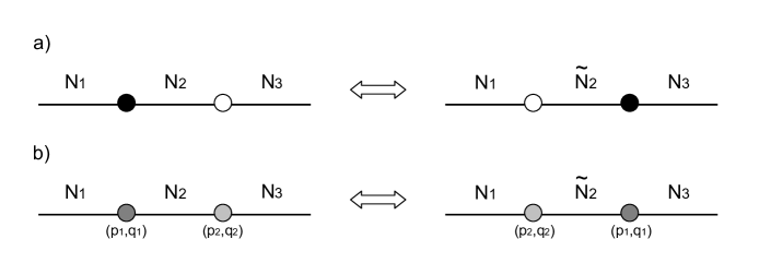
with MSL(2,)𝑀𝑆𝐿2M\in SL(2,\mathbb{Z}) and (p,q)superscript𝑝superscript𝑞(p^{\prime},q^{\prime}) given by (3.140) and arbitrary numbers N,N~𝑁~𝑁N,\widetilde{N} of eigenvalues {σj},{σ~j}subscript𝜎𝑗subscript~𝜎𝑗\{\sigma_{j}\},\{\widetilde{\sigma}_{j}\}. t𝑡t and tsuperscript𝑡t^{\prime} denote the deformation parameters of the (p,q)𝑝𝑞(p,q)- and (p,q)superscript𝑝superscript𝑞(p^{\prime},q^{\prime})-5branes respectively. Figure 12 displays the graphs of the two theories related by a local M𝑀M-duality. We have used the symbol =?superscript?\stackrel{{\scriptstyle?}}{{=}} to emphasize that we have not proven this relation. Indeed we will show that the relation holds only up to a phase.

Refer to caption
Figure 12: a) Part of a graph with a (p,q)superscript𝑝superscript𝑞(p^{\prime},q^{\prime})-5brane. b) Graph after the local M𝑀M-duality. The curly lines denote the presence of duality walls.

Checking the relation (3.150) for (p,q),(p,q){(1,0),(0,1),(1,k)}𝑝𝑞superscript𝑝superscript𝑞10011𝑘(p,q),(p^{\prime},q^{\prime})\in\{(1,0),(0,1),(1,k)\} constitutes a non-trivial test of the local SL(2,)𝑆𝐿2SL(2,\mathbb{Z}) dualities. For other (p,q)𝑝𝑞(p,q), (3.150) can be used to derive a matrix factor for an arbitrary (p,q)𝑝𝑞(p,q)-5brane with pq=1𝑝𝑞1p\wedge q=1.

3.3.1 (p,q)𝑝𝑞(p,q)-5brane matrix factor

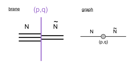
With p,q𝑝𝑞p,q being two integers such that p0𝑝0p\neq 0 and pq=1𝑝𝑞1p\wedge q=1, we propose the matrix model factor for a (p,q)𝑝𝑞(p,q) 5-brane (figure 13):

[pq]σσ~subscriptdelimited-[]𝑝𝑞𝜎~𝜎\displaystyle{\left[\begin{array}[]{c}p\\ q\end{array}\right]}_{\sigma\,\widetilde{\sigma}} =|p|μ(N!N~!)1/2e2πitp(jNσjjN~σ~j)eπiqp(jNσj2jN~σ~j2)i<jNsh[p1σij]i<jN~sh[p1σ~ij]i,jN,N~ch[p1(σiσ~j)],absentsuperscript𝑝𝜇superscript𝑁~𝑁12superscript𝑒2𝜋𝑖𝑡𝑝superscriptsubscript𝑗𝑁subscript𝜎𝑗superscriptsubscript𝑗~𝑁subscript~𝜎𝑗superscript𝑒𝜋𝑖𝑞𝑝superscriptsubscript𝑗𝑁superscriptsubscript𝜎𝑗2superscriptsubscript𝑗~𝑁superscriptsubscript~𝜎𝑗2superscriptsubscriptproduct𝑖𝑗𝑁shdelimited-[]superscript𝑝1subscript𝜎𝑖𝑗superscriptsubscriptproduct𝑖𝑗~𝑁shdelimited-[]superscript𝑝1subscript~𝜎𝑖𝑗superscriptsubscriptproduct𝑖𝑗𝑁~𝑁chdelimited-[]superscript𝑝1subscript𝜎𝑖subscript~𝜎𝑗\displaystyle=\frac{|p|^{-\mu}}{(N!\widetilde{N}!)^{1/2}}e^{-2\pi i\frac{t}{p}\left(\sum_{j}^{N}\sigma_{j}-\sum_{j}^{\widetilde{N}}\widetilde{\sigma}_{j}\right)}\ e^{\pi i\,\frac{q}{p}\left(\sum_{j}^{N}\sigma_{j}^{2}-\sum_{j}^{\widetilde{N}}\widetilde{\sigma}_{j}^{2}\right)}\ \frac{\prod_{i<j}^{N}\textrm{sh}[\,p^{-1}\sigma_{ij}]\ \prod_{i<j}^{\widetilde{N}}\textrm{sh}[\,p^{-1}\widetilde{\sigma}_{ij}]}{\prod_{i,j}^{N,\widetilde{N}}\textrm{ch}[\,p^{-1}(\sigma_{i}-\widetilde{\sigma}_{j})]}\ , (3.153)

where μ=N+N~2𝜇𝑁~𝑁2\mu=\frac{N+\widetilde{N}}{2}. In analogy with the previous 5-brane factors, t𝑡t should be associated to the position of the 5-brane in transverse space. This factor is compatible with the cases of NS5-brane and (1,k)1𝑘(1,k)-5brane factors (3.14) (3.20). It generalizes the proposal of [25] to the cases of unequal numbers of D3-segments ending on the left and right of the (p,q)𝑝𝑞(p,q)-5brane, NN~𝑁~𝑁N\neq\widetilde{N} and by the addition of the parameter t𝑡t dependence.

Refer to caption
Figure 13: (p,q)𝑝𝑞(p,q)-5brane building block and corresponding graph element in the graph description.

We have to show that this factor obeys the relation (3.150) and it is enough to consider the cases M=S𝑀𝑆M=S and M=T𝑀𝑇M=T and prove the inverted relations:

[qp]σσ~=?(S[pq]S1)σσ~,[pp+q]σσ~=?(T[pq]T1)σσ~,formulae-sequencesuperscript?subscriptdelimited-[]𝑞𝑝𝜎~𝜎subscript𝑆delimited-[]𝑝𝑞superscript𝑆1𝜎~𝜎superscript?subscriptdelimited-[]𝑝𝑝𝑞𝜎~𝜎subscript𝑇delimited-[]𝑝𝑞superscript𝑇1𝜎~𝜎\displaystyle{\left[\begin{array}[]{c}-q\\ p\end{array}\right]}_{\sigma\,\widetilde{\sigma}}\stackrel{{\scriptstyle?}}{{=}}\left(S{\left[\begin{array}[]{c}p\\ q\end{array}\right]}S^{-1}\right)_{\sigma\,\widetilde{\sigma}}\ ,\qquad{\left[\begin{array}[]{c}p\\ p+q\end{array}\right]}_{\sigma\,\widetilde{\sigma}}\stackrel{{\scriptstyle?}}{{=}}\left(T{\left[\begin{array}[]{c}p\\ q\end{array}\right]}T^{-1}\right)_{\sigma\,\widetilde{\sigma}}\ , (3.162)

Consider the sets of N𝑁N eigenvalues {σj}subscript𝜎𝑗\{\sigma_{j}\} and N~~𝑁\widetilde{N} eigenvalues {σ~j}subscript~𝜎𝑗\{\widetilde{\sigma}_{j}\} and a couple of coprime integers (p,q)𝑝𝑞(p,q) with p0𝑝0p\neq 0. For M=T𝑀𝑇M=T, we have

(T[pq]T1)σσ~=dNσdN~σ~eπiN12eπij=1Nσj2j=1Nδ(σjσj)subscript𝑇delimited-[]𝑝𝑞superscript𝑇1𝜎~𝜎superscript𝑑𝑁superscript𝜎superscript𝑑~𝑁superscript~𝜎superscript𝑒𝜋𝑖𝑁12superscript𝑒𝜋𝑖superscriptsubscript𝑗1𝑁superscriptsubscript𝜎𝑗2superscriptsubscriptproduct𝑗1𝑁𝛿subscript𝜎𝑗subscriptsuperscript𝜎𝑗\displaystyle\left(T{\left[\begin{array}[]{c}p\\ q\end{array}\right]}T^{-1}\right)_{\sigma\,\widetilde{\sigma}}=\int d^{N}\sigma^{\prime}d^{\widetilde{N}}\widetilde{\sigma}^{\prime}\ e^{\frac{\pi iN}{12}}\ e^{\pi i\sum_{j=1}^{N}\sigma_{j}^{2}}\ \prod_{j=1}^{N}\delta(\sigma_{j}-\sigma^{\prime}_{j}) (3.165)
.|p|μN!e2iπtp(jNσjjN~σ~j)eπiqp(jNσj2jN~σ~j)2i<jNsh[p1σij]i<jN~sh[p1σ~ij]i,jN,N~ch[p1(σiσ~j)]\displaystyle\qquad\ .\frac{|p|^{-\mu}}{N!}e^{-2i\pi\frac{t}{p}\left(\sum_{j}^{N}\sigma^{\prime}_{j}-\sum_{j}^{\widetilde{N}}\widetilde{\sigma}^{\prime}_{j}\right)}\ e^{\pi i\,\frac{q}{p}\left(\sum_{j}^{N}\sigma^{\prime}_{j}{}^{2}-\sum_{j}^{\widetilde{N}}\widetilde{\sigma}^{\prime}_{j}{}^{2}\right)}\ \frac{\prod_{i<j}^{N}\textrm{sh}[\,p^{-1}\sigma^{\prime}_{ij}]\ \prod_{i<j}^{\widetilde{N}}\textrm{sh}[\,p^{-1}\widetilde{\sigma}^{\prime}_{ij}]}{\prod_{i,j}^{N,\widetilde{N}}\textrm{ch}[\,p^{-1}(\sigma^{\prime}_{i}-\widetilde{\sigma}^{\prime}_{j})]}
.eπiN~12eπij=1N~σ~j2j=1N~δ(σ~jσ~j)\displaystyle\qquad\ .e^{-\frac{\pi i\widetilde{N}}{12}}\,e^{-\pi i\sum_{j=1}^{\widetilde{N}}\widetilde{\sigma}^{\prime}_{j}{}^{2}}\ \prod_{j=1}^{\widetilde{N}}\delta(\widetilde{\sigma}^{\prime}_{j}-\widetilde{\sigma}_{j})
=eπiΔ12|p|μN!e2iπtp(jNσjjN~σ~j)eπip+qp(jNσj2jN~σ~j)2i<jNsh[p1σij]i<jN~sh[p1σ~ij]i,jN,N~ch[p1(σiσ~j)]\displaystyle=e^{\frac{\pi i\Delta}{12}}\ \frac{|p|^{-\mu}}{N!}e^{-2i\pi\frac{t}{p}\left(\sum_{j}^{N}\sigma_{j}-\sum_{j}^{\widetilde{N}}\widetilde{\sigma}_{j}\right)}\ e^{\pi i\,\frac{p+q}{p}\left(\sum_{j}^{N}\sigma_{j}{}^{2}-\sum_{j}^{\widetilde{N}}\widetilde{\sigma}_{j}{}^{2}\right)}\ \frac{\prod_{i<j}^{N}\textrm{sh}[\,p^{-1}\sigma_{ij}]\ \prod_{i<j}^{\widetilde{N}}\textrm{sh}[\,p^{-1}\widetilde{\sigma}_{ij}]}{\prod_{i,j}^{N,\widetilde{N}}\textrm{ch}[\,p^{-1}(\sigma_{i}-\widetilde{\sigma}_{j})]}
=eπiΔ12[pp+q]σσ~,absentsuperscript𝑒𝜋𝑖Δ12subscriptdelimited-[]𝑝𝑝𝑞𝜎~𝜎\displaystyle=e^{\frac{\pi i\Delta}{12}}\ \ {\left[\begin{array}[]{c}p\\ p+q\end{array}\right]}_{\sigma\,\widetilde{\sigma}}\ , (3.168)

where μ=N+N~2𝜇𝑁~𝑁2\mu=\frac{N+\widetilde{N}}{2} and Δ=NN~Δ𝑁~𝑁\Delta=N-\widetilde{N}.

For M=S𝑀𝑆M=S the computation is given in appendix C.1. In total we obtain:

(S[pq]S1)σσ~subscript𝑆delimited-[]𝑝𝑞superscript𝑆1𝜎~𝜎\displaystyle\left(S{\left[\begin{array}[]{c}p\\ q\end{array}\right]}S^{-1}\right)_{\sigma\,\widetilde{\sigma}} =eπi12pqΔ(Δ21)eiπΔt2pq[qp]σσ~,pq0\displaystyle=\ e^{\frac{\pi i}{12\,pq}\Delta(\Delta^{2}-1)}\ e^{-\frac{i\pi\Delta t^{2}}{pq}}{\left[\begin{array}[]{c}-q\\ p\end{array}\right]}_{\sigma\,\widetilde{\sigma}}\quad,\quad pq\neq 0 (3.173)
(T[pq]T1)σσ~subscript𝑇delimited-[]𝑝𝑞superscript𝑇1𝜎~𝜎\displaystyle\left(T{\left[\begin{array}[]{c}p\\ q\end{array}\right]}T^{-1}\right)_{\sigma\,\widetilde{\sigma}} =eπiΔ12[pp+q]σσ~,p0.\displaystyle=\ e^{\frac{\pi i\Delta}{12}}\ \ {\left[\begin{array}[]{c}p\\ p+q\end{array}\right]}_{\sigma\,\widetilde{\sigma}}\hskip 71.13188pt,\quad p\neq 0\ . (3.178)

These relations have extra phases compared to the expected relations (3.162). The phases eπi12pqΔ(Δ21)superscript𝑒𝜋𝑖12𝑝𝑞ΔsuperscriptΔ21e^{\frac{\pi i}{12\,pq}\Delta(\Delta^{2}-1)} and eπiΔ12superscript𝑒𝜋𝑖Δ12e^{\frac{\pi i\Delta}{12}} are a priori irrelevant to the dynamics of the theories.111111It is possible that these phases are related to a change of frame of the Chern-Simons actions on S3superscript𝑆3S^{3} (see [6]). On the other hand the phase eiπΔt2pqsuperscript𝑒𝑖𝜋Δsuperscript𝑡2𝑝𝑞e^{-\frac{i\pi\Delta t^{2}}{pq}} can be attributed to the presence of a background Chern-Simons term for a weakly gauged U(1)𝑈1U(1) symmetry associated to the deformation parameter t𝑡t, with Chern-Simons level k=Δpq𝑘Δ𝑝𝑞k=\frac{\Delta}{pq}. It was shown in [27, 28] that the background Chern-Simons terms with integer coefficients are local counter-terms and characterize the ambiguity of the partition function. In the case at hand the Chern-Simons level ΔpqΔ𝑝𝑞\frac{\Delta}{pq} is generically fractional, but it is not clear what conclusions should be drawn from this observation, since the theories realized with (p,q)𝑝𝑞(p,q)-5branes are rather peculiar (non-Langrangian). However there are simpler cases when ΔpqΔ𝑝𝑞\frac{\Delta}{pq} is an integer. For instance when N=N~𝑁~𝑁N=\widetilde{N} or when |p|=|q|=1𝑝𝑞1|p|=|q|=1. In those cases the S𝑆S-action on the matrix factors is directly compatible with local S-duality of the brane configuration.


We are left with the untreated case when the relations involve D5-factors or D5¯¯D5\overline{\rm D5}-factors (p,q)=(0,±1)𝑝𝑞0plus-or-minus1(p,q)=(0,\pm 1). The D5-factor was given in (3.17) when N=N~𝑁~𝑁N=\widetilde{N}, but we have not specified it when NN~𝑁~𝑁N\neq\widetilde{N}, because it was not needed to describe the matrix models of quiver theories. Let us review first this simpler case. When N=N~𝑁~𝑁N=\widetilde{N}, we have directly:

(T[01]T1)σσ~subscript𝑇delimited-[]01superscript𝑇1𝜎~𝜎\displaystyle\left(T{\left[\begin{array}[]{c}0\\ 1\end{array}\right]}T^{-1}\right)_{\sigma\,\widetilde{\sigma}} =[01]σσ~,absentsubscriptdelimited-[]01𝜎~𝜎\displaystyle=\ {\left[\begin{array}[]{c}0\\ 1\end{array}\right]}_{\sigma\,\widetilde{\sigma}}\ , (3.183)

and

(S[01]S1)σσ~subscript𝑆delimited-[]01superscript𝑆1𝜎~𝜎\displaystyle\left(S{\left[\begin{array}[]{c}0\\ 1\end{array}\right]}S^{-1}\right)_{\sigma\,\widetilde{\sigma}} =dNσdNσ~e2πij=1NσjσjjNch(σjm)(w𝒮N(1)wN!jNδ(σjσ~w(j)))e2πij=1Nσ~jσ~jabsentsuperscript𝑑𝑁superscript𝜎superscript𝑑𝑁superscript~𝜎superscript𝑒2𝜋𝑖superscriptsubscript𝑗1𝑁subscript𝜎𝑗subscriptsuperscript𝜎𝑗superscriptsubscriptproduct𝑗𝑁chsubscriptsuperscript𝜎𝑗𝑚subscript𝑤subscript𝒮𝑁superscript1𝑤𝑁superscriptsubscriptproduct𝑗𝑁𝛿subscriptsuperscript𝜎𝑗subscriptsuperscript~𝜎𝑤𝑗superscript𝑒2𝜋𝑖superscriptsubscript𝑗1𝑁subscriptsuperscript~𝜎𝑗subscript~𝜎𝑗\displaystyle=\int d^{N}\sigma^{\prime}d^{N}\widetilde{\sigma}^{\prime}\,\frac{e^{2\pi i\sum_{j=1}^{N}\sigma_{j}\sigma^{\prime}_{j}}}{\prod_{j}^{N}\textrm{ch}(\sigma^{\prime}_{j}-m)}\,\left(\sum_{w\in\mathcal{S}_{N}}\frac{(-1)^{w}}{N!}\prod_{j}^{N}\delta(\sigma^{\prime}_{j}-\widetilde{\sigma}^{\prime}_{w(j)})\right)e^{-2\pi i\sum_{j=1}^{N}\widetilde{\sigma}^{\prime}_{j}\widetilde{\sigma}_{j}} (3.186)
=1N!w𝒮N(1)wdNσe2πij=1NσjσjjNch(σjm)e2πij=1Nσjσ~w(j)absent1𝑁subscript𝑤subscript𝒮𝑁superscript1𝑤superscript𝑑𝑁superscript𝜎superscript𝑒2𝜋𝑖superscriptsubscript𝑗1𝑁subscript𝜎𝑗subscriptsuperscript𝜎𝑗superscriptsubscriptproduct𝑗𝑁chsubscriptsuperscript𝜎𝑗𝑚superscript𝑒2𝜋𝑖superscriptsubscript𝑗1𝑁subscriptsuperscript𝜎𝑗subscript~𝜎𝑤𝑗\displaystyle=\frac{1}{N!}\sum_{w\in\mathcal{S}_{N}}(-1)^{w}\int d^{N}\sigma^{\prime}\ \frac{e^{2\pi i\sum_{j=1}^{N}\sigma_{j}\sigma^{\prime}_{j}}}{\prod_{j}^{N}\textrm{ch}(\sigma^{\prime}_{j}-m)}\ e^{-2\pi i\sum_{j=1}^{N}\sigma^{\prime}_{j}\widetilde{\sigma}_{w(j)}}
=e2πimjN(σjσ~j)N!w𝒮N(1)w1jNch(σjσ~w(j))absentsuperscript𝑒2𝜋𝑖𝑚superscriptsubscript𝑗𝑁subscript𝜎𝑗subscript~𝜎𝑗𝑁subscript𝑤subscript𝒮𝑁superscript1𝑤1superscriptsubscriptproduct𝑗𝑁chsubscript𝜎𝑗subscript~𝜎𝑤𝑗\displaystyle=\frac{e^{2\pi im\sum_{j}^{N}(\sigma_{j}-\widetilde{\sigma}_{j})}}{N!}\sum_{w\in\mathcal{S}_{N}}(-1)^{w}\frac{1}{\prod_{j}^{N}\textrm{ch}(\sigma_{j}-\widetilde{\sigma}_{w(j)})}
=[10]σσ~,absentsubscriptdelimited-[]10𝜎~𝜎\displaystyle={\left[\begin{array}[]{c}-1\\ 0\end{array}\right]}_{\sigma\,\widetilde{\sigma}}\ , (3.189)

where the last equality follows from the Cauchy formula (B.2). The D5¯¯D5\overline{\rm D5}-factor is defined as the D5-factor (3.17) with m𝑚m replaced by m𝑚-m, and the above relations hold with the roles of D5 and NS5 exchanged for D5¯¯D5\overline{\rm D5} and NS5¯¯NS5\overline{\rm NS5} . It will be important to test mirror symmetry on arbitrary quivers in section 4 to provide a D5-factor when NN~𝑁~𝑁N\neq\widetilde{N}, so we address this question now.

3.3.2 D5-factor with NN~𝑁~𝑁N\neq\widetilde{N}

To complete the picture it is possible to derive a D5-factor when NN~𝑁~𝑁N\neq\widetilde{N} (different numbers of D3-branes ending on the left and on the right of the D5-brane) by assuming the local S𝑆S-duality relation for arbitrary N,N~𝑁~𝑁N,\widetilde{N}:

[01]σσ~=(S[10]S1)σσ~.subscriptdelimited-[]01𝜎~𝜎subscript𝑆delimited-[]10superscript𝑆1𝜎~𝜎\displaystyle{\left[\begin{array}[]{c}0\\ 1\end{array}\right]}_{\sigma\,\widetilde{\sigma}}=\left(S{\left[\begin{array}[]{c}1\\ 0\end{array}\right]}S^{-1}\right)_{\sigma\,\widetilde{\sigma}}\ . (3.194)

Then we only need to check (3.150) for M=T𝑀𝑇M=T on this D5-factor to complete the proof that (3.150) holds for all MSL(2,)𝑀𝑆𝐿2M\in SL(2,\mathbb{Z}) and (p,q)𝑝𝑞(p,q)-factors. With Δ=NN~Δ𝑁~𝑁\Delta=N-\widetilde{N}, μ=N+N~2𝜇𝑁~𝑁2\mu=\frac{N+\widetilde{N}}{2} and N>N~𝑁~𝑁N>\widetilde{N}, the explicit D5-factor is

[01]σσ~subscriptdelimited-[]01𝜎~𝜎\displaystyle{\left[\begin{array}[]{c}0\\ 1\end{array}\right]}_{\sigma\,\widetilde{\sigma}} =(S[10]S1)σσ~absentsubscript𝑆delimited-[]10superscript𝑆1𝜎~𝜎\displaystyle=\ \left(S{\left[\begin{array}[]{c}1\\ 0\end{array}\right]}S^{-1}\right)_{\sigma\,\widetilde{\sigma}}
=dNτdN~τ~e2πijNσjτj[10]ττ~e2πijN~τ~jσ~jabsentsuperscript𝑑𝑁𝜏superscript𝑑~𝑁~𝜏superscript𝑒2𝜋𝑖superscriptsubscript𝑗𝑁subscript𝜎𝑗subscript𝜏𝑗subscriptdelimited-[]10𝜏~𝜏superscript𝑒2𝜋𝑖superscriptsubscript𝑗~𝑁subscript~𝜏𝑗subscript~𝜎𝑗\displaystyle=\int d^{N}\tau d^{\widetilde{N}}\widetilde{\tau}\ e^{2\pi i\sum_{j}^{N}\sigma_{j}\tau_{j}}\ {\left[\begin{array}[]{c}1\\ 0\end{array}\right]}_{\tau\widetilde{\tau}}\ e^{-2\pi i\sum_{j}^{\widetilde{N}}\widetilde{\tau}_{j}\widetilde{\sigma}_{j}}
=(1)ΔN~(N!N~!)1/2w𝒮N(1)wdNτdN~τ~e2πijNτj(σjm)e2πijN~τ~j(σ~jm)absentsuperscript1Δ~𝑁superscript𝑁~𝑁12subscript𝑤subscript𝒮𝑁superscript1𝑤superscript𝑑𝑁𝜏superscript𝑑~𝑁~𝜏superscript𝑒2𝜋𝑖superscriptsubscript𝑗𝑁subscript𝜏𝑗subscript𝜎𝑗𝑚superscript𝑒2𝜋𝑖superscriptsubscript𝑗~𝑁subscript~𝜏𝑗subscript~𝜎𝑗𝑚\displaystyle=\frac{(-1)^{\Delta\widetilde{N}}}{(N!\widetilde{N}!)^{1/2}}\sum_{w\in\mathcal{S}_{N}}(-1)^{w}\int d^{N}\tau d^{\widetilde{N}}\widetilde{\tau}\ e^{2\pi i\sum_{j}^{N}\tau_{j}(\sigma_{j}-m)}\ e^{-2\pi i\sum_{j}^{\widetilde{N}}\widetilde{\tau}_{j}(\widetilde{\sigma}_{j}-m)}
.j=1N~eπΔ(τw(j)τ~j)ch(τw(j)τ~j)j=N~+1Ne2πτw(j)(μ+12j)\displaystyle\hskip 113.81102pt.\prod_{j=1}^{\widetilde{N}}\frac{e^{-\pi\Delta(\tau_{w(j)}-\widetilde{\tau}_{j})}}{\textrm{ch}(\tau_{w(j)}-\widetilde{\tau}_{j})}\prod_{j=\widetilde{N}+1}^{N}e^{2\pi\tau_{w(j)}\left(\mu+\frac{1}{2}-j\right)}

where we used the generalized Cauchy formula (B.3) to replace the NS5 factor. m𝑚m is the 5-brane deformation parameter. The result factorizes into a product of N~~𝑁\widetilde{N} single integrals over the τ~jsubscript~𝜏𝑗\widetilde{\tau}_{j}. These integrals are not convergent, however it is possible to evaluate them as the analytical continuation to complex y𝑦y of the standard integral 𝑑xe2πixychx=1chydifferential-d𝑥superscript𝑒2𝜋𝑖𝑥𝑦ch𝑥1ch𝑦\int dx\,\frac{e^{2\pi i\,x\,y}}{\textrm{ch}\,x}=\frac{1}{\textrm{ch}\,y}.121212A more rigorous approach is to consider expanding the integrand as eπΔxjch(xj)=eπ(Δ1)xjeπ(Δ3)xj++(1)Δ/2ch(xj)superscript𝑒𝜋Δsubscript𝑥𝑗chsubscript𝑥𝑗superscript𝑒𝜋Δ1subscript𝑥𝑗superscript𝑒𝜋Δ3subscript𝑥𝑗superscript1Δ2chsubscript𝑥𝑗\frac{e^{-\pi\Delta x_{j}}}{\textrm{ch}(x_{j})}=e^{\pi(\Delta-1)x_{j}}-e^{\pi(\Delta-3)x_{j}}+\cdots+\frac{(-1)^{\Delta/2}}{\textrm{ch}(x_{j})} for Δ2Δ2\Delta\in 2\mathbb{Z}, or eπΔxjch(xj)=eπ(Δ1)xjeπ(Δ3)xj++(1)(Δ1)/22(1+th(xj))superscript𝑒𝜋Δsubscript𝑥𝑗chsubscript𝑥𝑗superscript𝑒𝜋Δ1subscript𝑥𝑗superscript𝑒𝜋Δ3subscript𝑥𝑗superscript1Δ1221thsubscript𝑥𝑗\frac{e^{-\pi\Delta x_{j}}}{\textrm{ch}(x_{j})}=e^{\pi(\Delta-1)x_{j}}-e^{\pi(\Delta-3)x_{j}}+\cdots+\frac{(-1)^{(\Delta-1)/2}}{2}(1+\textrm{th}(x_{j})) for Δ2+1Δ21\Delta\in 2\mathbb{Z}+1, where xj=τw(j)τ~jsubscript𝑥𝑗subscript𝜏𝑤𝑗subscript~𝜏𝑗x_{j}=\tau_{w(j)}-\widetilde{\tau}_{j}, and then notice that all contributions vanish because of the τjsubscript𝜏𝑗\tau_{j} anti-symmetrization, except the contribution from (1)Δ/2ch(xj)superscript1Δ2chsubscript𝑥𝑗\frac{(-1)^{\Delta/2}}{\textrm{ch}(x_{j})} or (1)(Δ1)/22th(xj)superscript1Δ122thsubscript𝑥𝑗\frac{(-1)^{(\Delta-1)/2}}{2}\textrm{th}(x_{j}). The integrals over these factors are convergent and give the same result as the analytical continuation proposed in the text.

=(1)ΔN~(N!N~!)1/2w𝒮N(1)wdNτe2πijNτj(σjm)j=1N~e2πi(mσ~j)τw(j)ch(mσ~jiΔ2)j=N~+1Ne2πτw(j)(μ+12j)absentsuperscript1Δ~𝑁superscript𝑁~𝑁12subscript𝑤superscript𝒮𝑁superscript1𝑤superscript𝑑𝑁𝜏superscript𝑒2𝜋𝑖superscriptsubscript𝑗𝑁subscript𝜏𝑗subscript𝜎𝑗𝑚superscriptsubscriptproduct𝑗1~𝑁superscript𝑒2𝜋𝑖𝑚subscript~𝜎𝑗subscript𝜏𝑤𝑗ch𝑚subscript~𝜎𝑗𝑖Δ2superscriptsubscriptproduct𝑗~𝑁1𝑁superscript𝑒2𝜋subscript𝜏𝑤𝑗𝜇12𝑗\displaystyle=\frac{(-1)^{\Delta\widetilde{N}}}{(N!\widetilde{N}!)^{1/2}}\sum_{w\in\mathcal{S}^{N}}(-1)^{w}\int d^{N}\tau\ e^{2\pi i\sum_{j}^{N}\tau_{j}(\sigma_{j}-m)}\ \prod_{j=1}^{\widetilde{N}}\frac{e^{2\pi i(m-\widetilde{\sigma}_{j})\tau_{w(j)}}}{\textrm{ch}(m-\widetilde{\sigma}_{j}-i\frac{\Delta}{2})}\ \prod_{j=\widetilde{N}+1}^{N}e^{2\pi\tau_{w(j)}\left(\mu+\frac{1}{2}-j\right)}
=(1)ΔN~(N!N~!)1/2j=1N~ch(σ~jm+iΔ2)w𝒮N(1)wdNτj=1N~e2πiτj(σw(j)σ~j)j=N~+1Ne2πiτj(σw(j)mi(μ+12j))absentsuperscript1Δ~𝑁superscript𝑁~𝑁12superscriptsubscriptproduct𝑗1~𝑁chsubscript~𝜎𝑗𝑚𝑖Δ2subscript𝑤superscript𝒮𝑁superscript1𝑤superscript𝑑𝑁𝜏superscriptsubscriptproduct𝑗1~𝑁superscript𝑒2𝜋𝑖subscript𝜏𝑗subscript𝜎𝑤𝑗subscript~𝜎𝑗superscriptsubscriptproduct𝑗~𝑁1𝑁superscript𝑒2𝜋𝑖subscript𝜏𝑗subscript𝜎𝑤𝑗𝑚𝑖𝜇12𝑗\displaystyle=\frac{(-1)^{\Delta\widetilde{N}}\,(N!\widetilde{N}!)^{-1/2}}{\prod_{j=1}^{\widetilde{N}}\textrm{ch}(\widetilde{\sigma}_{j}-m+i\frac{\Delta}{2})}\sum_{w\in\mathcal{S}^{N}}(-1)^{w}\int d^{N}\tau\ \prod_{j=1}^{\widetilde{N}}e^{2\pi i\tau_{j}(\sigma_{w(j)}-\widetilde{\sigma}_{j})}\prod_{j=\widetilde{N}+1}^{N}e^{2\pi i\tau_{j}\left(\sigma_{w(j)}-m-i\left(\mu+\frac{1}{2}-j\right)\right)}

where we have relabelled τw(j)τjsubscript𝜏𝑤𝑗subscript𝜏𝑗\tau_{w(j)}\rightarrow\tau_{j} in each integral. We are left with the integrations over the τjsubscript𝜏𝑗\tau_{j} which correspond to usual δ𝛿\delta functions and special δ𝛿\delta functions of a complex variable that we denote δ^(.)\hat{\delta}(.).

=(N!N~!)1/2j=1N~ch(σ~jmiΔ2)w𝒮N(1)wj=1N~δ(σw(j)σ~j)j=N~+1Nδ^[σw(j)mjN~(Δ)]absentsuperscript𝑁~𝑁12superscriptsubscriptproduct𝑗1~𝑁chsubscript~𝜎𝑗𝑚𝑖Δ2subscript𝑤superscript𝒮𝑁superscript1𝑤superscriptsubscriptproduct𝑗1~𝑁𝛿subscript𝜎𝑤𝑗subscript~𝜎𝑗superscriptsubscriptproduct𝑗~𝑁1𝑁^𝛿delimited-[]subscript𝜎𝑤𝑗subscriptsuperscript𝑚Δ𝑗~𝑁\displaystyle=\frac{(N!\widetilde{N}!)^{-1/2}}{\prod_{j=1}^{\widetilde{N}}\textrm{ch}\left(\widetilde{\sigma}_{j}-m-i\frac{\Delta}{2}\right)}\ \sum_{w\in\mathcal{S}^{N}}(-1)^{w}\prod_{j=1}^{\widetilde{N}}\delta(\sigma_{w(j)}-\widetilde{\sigma}_{j})\ \prod_{j=\widetilde{N}+1}^{N}\hat{\delta}[\sigma_{w(j)}-m^{(\Delta)}_{j-\widetilde{N}}]

with mj(Δ)=m+i(Δ+12j)subscriptsuperscript𝑚Δ𝑗𝑚𝑖Δ12𝑗m^{(\Delta)}_{j}=m+i\left(\frac{\Delta+1}{2}-j\right) for j=1,,Δ𝑗1Δj=1,\cdots,\Delta and we have used ch(x+in)=(1)nchxch𝑥𝑖𝑛superscript1𝑛ch𝑥\textrm{ch}(x+in)=(-1)^{n}\textrm{ch}\,x, for n𝑛n\in\mathbb{Z}. The δ^^𝛿\hat{\delta} must be defined as a special distribution that generalizes the usual δ𝛿\delta distribution for the class of integrals that we treat. 131313When dealing with divergent matrix integrals, a standard recipe is to rely on analytic continuation of the integrals [36] with respect to some parameters of the integrand. In our case such an analytical continuation is not possible because the the function to be analytically continued is the Dirac delta function. This is why we do not speak about analytic continuation, but about ”generalization” of the delta function. It might be surprising that we have to define such an exotic object, however one should remember that this defines a matrix factor for a D5-brane with NN~𝑁~𝑁N\neq\widetilde{N}, which is not a natural factor arising in the matrix model of a gauge theory. When gluing together all the factors of a ”good” matrix model, one should be able to integrate out the D5-factors and remain with a standard converging matrix model. Formally it should correspond to:

δ^(y)=𝑑xe2πiyx,^𝛿𝑦subscriptdifferential-d𝑥superscript𝑒2𝜋𝑖𝑦𝑥\displaystyle\hat{\delta}(y)=\int_{\mathbb{R}}dx\ e^{2\pi iyx}\ , (3.195)

for y𝑦y\in\mathbb{C}. A heuristic computation presented in appendix A lead us to the following definition. For z0subscript𝑧0z_{0}\in\mathbb{Z}, δ^z0δ^(.z0)\hat{\delta}_{z_{0}}\equiv\hat{\delta}(\,.\,-z_{0}) is defined by its action on a meromorphic function f𝑓f with simple poles (away from z0subscript𝑧0z_{0}):

𝑑xδ^(xz0)f(x)subscriptdifferential-d𝑥^𝛿𝑥subscript𝑧0𝑓𝑥\displaystyle\int_{\mathbb{R}}dx\ \hat{\delta}(x-z_{0})f(x) =f(z0)+ 2πiϵ(z0)jδ^(ujz0)f^(uj)absent𝑓subscript𝑧02𝜋𝑖italic-ϵsubscript𝑧0subscript𝑗^𝛿subscript𝑢𝑗subscript𝑧0^𝑓subscript𝑢𝑗\displaystyle=f(z_{0})\ +\ 2\pi i\epsilon(z_{0})\sum_{j}\hat{\delta}(u_{j}-z_{0})\hat{f}(u_{j}) (3.196)

where ϵ(z0)=italic-ϵsubscript𝑧0absent\epsilon(z_{0})=\ sgn(Im(z0))Imsubscript𝑧0({\rm Im}(z_{0})), ujsubscript𝑢𝑗u_{j} are the poles of f𝑓f in the region 0Im(u)Im(z0)0Im𝑢Imsubscript𝑧00\leq{\rm Im}(u)\leq{\rm Im}(z_{0}) (or Im(z0)Im(u)0Imsubscript𝑧0Im𝑢0{\rm Im}(z_{0})\leq{\rm Im}(u)\leq 0). When 0<|Im(uj)|<|Im(z0)|0Imsubscript𝑢𝑗Imsubscript𝑧00<|{\rm Im}(u_{j})|<|{\rm Im}(z_{0})|, f^(uj)^𝑓subscript𝑢𝑗\hat{f}(u_{j}) is the residue at the pole ujsubscript𝑢𝑗u_{j}, when Im(uj)=0Imsubscript𝑢𝑗0{\rm Im}(u_{j})=0 or Im(uj)=Im(z0)Imsubscript𝑢𝑗Imsubscript𝑧0{\rm Im}(u_{j})={\rm Im}(z_{0}), f^(uj)^𝑓subscript𝑢𝑗\hat{f}(u_{j}) is half the residue at the pole ujsubscript𝑢𝑗u_{j}. We give details about these exotic δ^^𝛿\hat{\delta} in appendix A.

To conclude we have obtained a generalized D5-factor:

[01]σσ~=(N!N~!)1/2j=1N~ch(σ~jmiΔ2)w𝒮N(1)wj=1N~δ(σw(j)σ~j)j=N~+1Nδ^[σw(j)mjN~(Δ)]subscriptdelimited-[]01𝜎~𝜎superscript𝑁~𝑁12superscriptsubscriptproduct𝑗1~𝑁chsubscript~𝜎𝑗𝑚𝑖Δ2subscript𝑤superscript𝒮𝑁superscript1𝑤superscriptsubscriptproduct𝑗1~𝑁𝛿subscript𝜎𝑤𝑗subscript~𝜎𝑗superscriptsubscriptproduct𝑗~𝑁1𝑁^𝛿delimited-[]subscript𝜎𝑤𝑗subscriptsuperscript𝑚Δ𝑗~𝑁\displaystyle{\left[\begin{array}[]{c}0\\ 1\end{array}\right]}_{\sigma\,\widetilde{\sigma}}=\frac{(N!\widetilde{N}!)^{-1/2}}{\prod_{j=1}^{\widetilde{N}}\textrm{ch}\left(\widetilde{\sigma}_{j}-m-i\frac{\Delta}{2}\right)}\ \sum_{w\in\mathcal{S}^{N}}(-1)^{w}\prod_{j=1}^{\widetilde{N}}\delta(\sigma_{w(j)}-\widetilde{\sigma}_{j})\ \prod_{j=\widetilde{N}+1}^{N}\hat{\delta}\big{[}\sigma_{w(j)}-m^{(\Delta)}_{j-\widetilde{N}}\big{]} (3.199) withmj(Δ)=m+iΔ2j+12,forNN~formulae-sequencewithsubscriptsuperscript𝑚Δ𝑗𝑚𝑖Δ2𝑗12for𝑁~𝑁\displaystyle\quad\textrm{with}\quad m^{(\Delta)}_{j}=m+i\,\frac{\Delta-2j+1}{2}\ ,\quad{\rm for}\quad N\geq\widetilde{N} (3.200)

For N=N~𝑁~𝑁N=\widetilde{N} it reduces to (3.17) with mass parameter m𝑚m. When N<N~𝑁~𝑁N<\widetilde{N} the D5-factor is given by the above formula with NN~𝑁~𝑁N\leftrightarrow\widetilde{N}, σσ~𝜎~𝜎\sigma\leftrightarrow-\widetilde{\sigma} and mm𝑚𝑚m\rightarrow-m. This yields

[01]σσ~=(N!N~!)1/2j=1Nch(σ~jm+iΔ~2)w𝒮N~(1)wj=1Nδ(σ~w(j)σj)j=N+1N~δ^(σ~w(j)mjN(Δ~)),subscriptdelimited-[]01𝜎~𝜎superscript𝑁~𝑁12superscriptsubscriptproduct𝑗1𝑁chsubscript~𝜎𝑗𝑚𝑖~Δ2subscript𝑤superscript𝒮~𝑁superscript1𝑤superscriptsubscriptproduct𝑗1𝑁𝛿subscript~𝜎𝑤𝑗subscript𝜎𝑗superscriptsubscriptproduct𝑗𝑁1~𝑁^𝛿subscript~𝜎𝑤𝑗subscriptsuperscript𝑚~Δ𝑗𝑁\displaystyle{\left[\begin{array}[]{c}0\\ 1\end{array}\right]}_{\sigma\,\widetilde{\sigma}}=\frac{(N!\widetilde{N}!)^{-1/2}}{\prod_{j=1}^{N}\textrm{ch}\left(\widetilde{\sigma}_{j}-m+i\frac{\widetilde{\Delta}}{2}\right)}\ \sum_{w\in\mathcal{S}^{\widetilde{N}}}(-1)^{w}\prod_{j=1}^{N}\delta(\widetilde{\sigma}_{w(j)}-\sigma_{j})\ \prod_{j=N+1}^{\widetilde{N}}\hat{\delta}(\widetilde{\sigma}_{w(j)}-m^{(\widetilde{\Delta})\ast}_{j-N})\ , (3.203)

with Δ~=N~N~Δ~𝑁𝑁\widetilde{\Delta}=\widetilde{N}-N and \ast denotes complex conjugation.


Let us see what becomes of the relations (3.162) for the D5-factor.

(S[01]S1)σσ~subscript𝑆delimited-[]01superscript𝑆1𝜎~𝜎\displaystyle\left(S{\left[\begin{array}[]{c}0\\ 1\end{array}\right]}S^{-1}\right)_{\sigma\,\widetilde{\sigma}} =(S2[10]S2)σσ~=((1)[10](1))σσ~=[10]σσ~.absentsubscriptsuperscript𝑆2delimited-[]10superscript𝑆2𝜎~𝜎subscript1delimited-[]101𝜎~𝜎subscriptdelimited-[]10𝜎~𝜎\displaystyle=\left(S^{2}{\left[\begin{array}[]{c}1\\ 0\end{array}\right]}S^{-2}\right)_{\sigma\,\widetilde{\sigma}}=\left((-1){\left[\begin{array}[]{c}1\\ 0\end{array}\right]}(-1)\right)_{\sigma\,\widetilde{\sigma}}={\left[\begin{array}[]{c}-1\\ 0\end{array}\right]}_{\sigma\,\widetilde{\sigma}}\ . (3.212)

This equality can also be checked directly using the D5-factor we have derived. Then for NN~𝑁~𝑁N\geq\widetilde{N},

(T[01]T1)σσ~=eπiΔ12dNτdN~τ~eπij=1Nσj2j=1Nδ(σjτj)[01]ττ~eπij=1N~τ~j2j=1N~δ(τ~jσ~j)subscript𝑇delimited-[]01superscript𝑇1𝜎~𝜎superscript𝑒𝜋𝑖Δ12superscript𝑑𝑁𝜏superscript𝑑~𝑁~𝜏superscript𝑒𝜋𝑖superscriptsubscript𝑗1𝑁superscriptsubscript𝜎𝑗2superscriptsubscriptproduct𝑗1𝑁𝛿subscript𝜎𝑗subscript𝜏𝑗subscriptdelimited-[]01𝜏~𝜏superscript𝑒𝜋𝑖superscriptsubscript𝑗1~𝑁superscriptsubscript~𝜏𝑗2superscriptsubscriptproduct𝑗1~𝑁𝛿subscript~𝜏𝑗subscript~𝜎𝑗\displaystyle\left(T{\left[\begin{array}[]{c}0\\ 1\end{array}\right]}T^{-1}\right)_{\sigma\,\widetilde{\sigma}}=\ e^{\frac{\pi i\Delta}{12}}\int d^{N}\tau d^{\widetilde{N}}\widetilde{\tau}\ e^{\pi i\sum_{j=1}^{N}\sigma_{j}^{2}}\ \prod_{j=1}^{N}\delta(\sigma_{j}-\tau_{j})\ {\left[\begin{array}[]{c}0\\ 1\end{array}\right]}_{\tau\,\widetilde{\tau}}\ e^{-\pi i\sum_{j=1}^{\widetilde{N}}\widetilde{\tau}_{j}^{2}}\ \prod_{j=1}^{\widetilde{N}}\delta(\widetilde{\tau}_{j}-\widetilde{\sigma}_{j}) (3.217)
=eπiΔ12eπij=1Nσj2[01]σσ~eπij=1N~σ~j2absentsuperscript𝑒𝜋𝑖Δ12superscript𝑒𝜋𝑖superscriptsubscript𝑗1𝑁superscriptsubscript𝜎𝑗2subscriptdelimited-[]01𝜎~𝜎superscript𝑒𝜋𝑖superscriptsubscript𝑗1~𝑁superscriptsubscript~𝜎𝑗2\displaystyle=\ e^{\frac{\pi i\Delta}{12}}\ e^{\pi i\sum_{j=1}^{N}\sigma_{j}^{2}}\ {\left[\begin{array}[]{c}0\\ 1\end{array}\right]}_{\sigma\,\widetilde{\sigma}}\ e^{-\pi i\sum_{j=1}^{\widetilde{N}}\widetilde{\sigma}_{j}^{2}} (3.220)
=eπiΔ12(N!N~!)1/2j=1N~ch(σ~jmiΔ2)w𝒮N(1)wj=1N~δ(σw(j)σ~j)j=N~+1Nδ^[σw(j)mjN~(Δ)]eπijΔ(mj(Δ))2absentsuperscript𝑒𝜋𝑖Δ12superscript𝑁~𝑁12superscriptsubscriptproduct𝑗1~𝑁chsubscript~𝜎𝑗𝑚𝑖Δ2subscript𝑤superscript𝒮𝑁superscript1𝑤superscriptsubscriptproduct𝑗1~𝑁𝛿subscript𝜎𝑤𝑗subscript~𝜎𝑗superscriptsubscriptproduct𝑗~𝑁1𝑁^𝛿delimited-[]subscript𝜎𝑤𝑗subscriptsuperscript𝑚Δ𝑗~𝑁superscript𝑒𝜋𝑖superscriptsubscript𝑗Δsuperscriptsubscriptsuperscript𝑚Δ𝑗2\displaystyle=\frac{e^{\frac{\pi i\Delta}{12}}\,(N!\widetilde{N}!)^{-1/2}}{\prod_{j=1}^{\widetilde{N}}\textrm{ch}\left(\widetilde{\sigma}_{j}-m-i\frac{\Delta}{2}\right)}\ \sum_{w\in\mathcal{S}^{N}}(-1)^{w}\prod_{j=1}^{\widetilde{N}}\delta(\sigma_{w(j)}-\widetilde{\sigma}_{j})\ \prod_{j=\widetilde{N}+1}^{N}\hat{\delta}\big{[}\sigma_{w(j)}-m^{(\Delta)}_{j-\widetilde{N}}\big{]}\ e^{\pi i\sum_{j}^{\Delta}(m^{(\Delta)}_{j}{})^{2}}
=eπiΔ12eπi12Δ(Δ21)eπiΔm2[01]σσ~,absentsuperscript𝑒𝜋𝑖Δ12superscript𝑒𝜋𝑖12ΔsuperscriptΔ21superscript𝑒𝜋𝑖Δsuperscript𝑚2subscriptdelimited-[]01𝜎~𝜎\displaystyle=e^{\frac{\pi i\Delta}{12}}\,e^{\frac{\pi i}{12}\Delta(\Delta^{2}-1)}\,e^{\pi i\Delta m^{2}}\ {\left[\begin{array}[]{c}0\\ 1\end{array}\right]}_{\sigma\,\widetilde{\sigma}}\ , (3.223)

at the third line we have used the property (A.3). The relations (3.178) are then completed with:

(S[10]S1)σσ~subscript𝑆delimited-[]10superscript𝑆1𝜎~𝜎\displaystyle\left(S{\left[\begin{array}[]{c}1\\ 0\end{array}\right]}S^{-1}\right)_{\sigma\,\widetilde{\sigma}} =[01]σσ~,(S[01]S1)σσ~=[10]σσ~\displaystyle=\ {\left[\begin{array}[]{c}0\\ 1\end{array}\right]}_{\sigma\,\widetilde{\sigma}}\quad,\quad\left(S{\left[\begin{array}[]{c}0\\ 1\end{array}\right]}S^{-1}\right)_{\sigma\,\widetilde{\sigma}}=\ {\left[\begin{array}[]{c}-1\\ 0\end{array}\right]}_{\sigma\,\widetilde{\sigma}} (3.232)
(T[01]T1)σσ~subscript𝑇delimited-[]01superscript𝑇1𝜎~𝜎\displaystyle\left(T{\left[\begin{array}[]{c}0\\ 1\end{array}\right]}T^{-1}\right)_{\sigma\,\widetilde{\sigma}} =eπi12Δ3eπiΔm2[01]σσ~.absentsuperscript𝑒𝜋𝑖12superscriptΔ3superscript𝑒𝜋𝑖Δsuperscript𝑚2subscriptdelimited-[]01𝜎~𝜎\displaystyle=\ e^{\frac{\pi i}{12}\Delta^{3}}\ e^{\pi i\Delta m^{2}}\ {\left[\begin{array}[]{c}0\\ 1\end{array}\right]}_{\sigma\,\widetilde{\sigma}}\ . (3.237)

The phase eπiΔm2superscript𝑒𝜋𝑖Δsuperscript𝑚2e^{\pi i\Delta m^{2}} accounts for a background Chern-Simons term with integer level ΔΔ\Delta, which does not affect the physics of the theory [27, 28].
The dualities we will test involve theories realized with D5-, NS5- and (1,±1)1plus-or-minus1(1,\pm 1)-5branes and thus the additional phases will contain only unphysical integer level background CS terms.

3.4 Tests of SL(2,\mathbb{Z}) dualities

In this section we show how the machinery of local SL(2,)𝑆𝐿2SL(2,\mathbb{Z}) transformations produces a powerful test of SL(2,)𝑆𝐿2SL(2,\mathbb{Z}) dualities, by matching the exact partition functions on S3superscript𝑆3S^{3} of dual SCFTs.

Let us first re-derive the test of mirror symmetry for Yang-Mills circular quivers with nodes of equal rank presented in [7]. Consider a circular quiver theory A𝐴A with nodes of equal ranks. It has a gauge group GA=j=1P^U(N)subscript𝐺𝐴superscriptsubscriptproduct𝑗1^𝑃𝑈𝑁G_{A}=\prod_{j=1}^{\widehat{P}}U(N) with bifundamental hypermultiplets and Mjsubscript𝑀𝑗M_{j} fundamental hypermultiplets in the j𝑗jth node. Its brane realization involves N𝑁N D3-branes on a circle crossing a sequence of NS5 and D5-branes. The mirror-dual theory B is realized by the S-dual brane configuration changing the NS5 into D5-branes and the D5 into NS5¯¯NS5\overline{\rm NS5}-branes. Theory B is also a Yang-Mills circular quiver, with gauge group GB=j=1PU(N)subscript𝐺𝐵superscriptsubscriptproduct𝑗1𝑃𝑈𝑁G_{B}=\prod_{j=1}^{P}U(N) and M~jsubscript~𝑀𝑗\widetilde{M}_{j} fundamental hypermultiplets in the j𝑗jth node. The relations between the A and B quivers data can be read from the brane configurations. The partition function of theory A is given by its sequence of NS5 and D5 factors:

ZAsubscript𝑍𝐴\displaystyle Z_{A} =Tr[10][01](N)[01](N)[10](N)(N)[01](N)(N)\displaystyle=\textrm{Tr}\ {\left[\begin{array}[]{c}1\\ 0\end{array}\right]}{}_{(N)}{\left[\begin{array}[]{c}0\\ 1\end{array}\right]}{}_{(N)}{\left[\begin{array}[]{c}0\\ 1\end{array}\right]}{}_{(N)}{\left[\begin{array}[]{c}1\\ 0\end{array}\right]}{}_{(N)}\cdots{}_{(N)}{\left[\begin{array}[]{c}0\\ 1\end{array}\right]}{}_{(N)} (3.248)
=Tr[10][01][01][10][01].absentTrdelimited-[]10delimited-[]01delimited-[]01delimited-[]10delimited-[]01\displaystyle=\textrm{Tr}\ {\left[\begin{array}[]{c}1\\ 0\end{array}\right]}{\left[\begin{array}[]{c}0\\ 1\end{array}\right]}{\left[\begin{array}[]{c}0\\ 1\end{array}\right]}{\left[\begin{array}[]{c}1\\ 0\end{array}\right]}\cdots{\left[\begin{array}[]{c}0\\ 1\end{array}\right]}\ . (3.259)

Each 5-brane factor can be replaced by its local S𝑆S-dual using (3.150):

ZAsubscript𝑍𝐴\displaystyle Z_{A} =TrS1[01]SS1[10]SS1[10]SS1[01]SS1[10]SabsentTrsuperscript𝑆1delimited-[]01𝑆superscript𝑆1delimited-[]10𝑆superscript𝑆1delimited-[]10𝑆superscript𝑆1delimited-[]01𝑆superscript𝑆1delimited-[]10𝑆\displaystyle=\textrm{Tr}\ S^{-1}{\left[\begin{array}[]{c}0\\ 1\end{array}\right]}S\,S^{-1}{\left[\begin{array}[]{c}-1\\ 0\end{array}\right]}S\,S^{-1}{\left[\begin{array}[]{c}-1\\ 0\end{array}\right]}S\,S^{-1}{\left[\begin{array}[]{c}0\\ 1\end{array}\right]}S\,\cdots\,S^{-1}{\left[\begin{array}[]{c}-1\\ 0\end{array}\right]}S (3.270)
=Tr[01][10][10][01][10]absentTrdelimited-[]01delimited-[]10delimited-[]10delimited-[]01delimited-[]10\displaystyle=\textrm{Tr}\ {\left[\begin{array}[]{c}0\\ 1\end{array}\right]}\,{\left[\begin{array}[]{c}-1\\ 0\end{array}\right]}\,{\left[\begin{array}[]{c}-1\\ 0\end{array}\right]}\,{\left[\begin{array}[]{c}0\\ 1\end{array}\right]}\,\cdots\,{\left[\begin{array}[]{c}-1\\ 0\end{array}\right]} (3.281)
=ZB,absentsubscript𝑍𝐵\displaystyle=Z_{B}\ , (3.282)

where the second equality follows from (SS1)σσ~=1σσ~subscript𝑆superscript𝑆1𝜎~𝜎subscript1𝜎~𝜎(S\,S^{-1})_{\sigma\widetilde{\sigma}}=1_{\sigma\widetilde{\sigma}}. The matrix model obtained after these simple manipulations is the matrix model for the partition function ZBsubscript𝑍𝐵Z_{B} of the S𝑆S-dual theory B𝐵B. The parameter tjsubscript𝑡𝑗t_{j} of the j𝑗j-th 5brane in the sequence of ZAsubscript𝑍𝐴Z_{A} is mapped to the parameter t^jsubscript^𝑡𝑗\hat{t}_{j} of the j𝑗j-th 5brane in the sequence of ZBsubscript𝑍𝐵Z_{B}. This means that the mass parameters misubscript𝑚𝑖m_{i} and tjsubscript𝑡𝑗t_{j}, associated to D5- and NS5-branes, are exchanged with the parameters t^isubscript^𝑡𝑖\hat{t}_{i} and m^jsubscript^𝑚𝑗\hat{m}_{j} of the mirror theory, associated with NS5¯¯NS5\overline{\rm NS5} and D5-branes. For these quiver theories, S𝑆S-duality coincides with mirror symmetry. Theories A and B in figure 14 are an example of YM mirror theories.
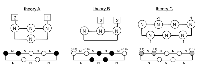
Refer to caption
Figure 14: Triplet of SL(2,)𝑆𝐿2SL(2,\mathbb{Z}) dual theories. Theories A and B are Yang-Mills quiver SCFTs, while theory C is a Chern-Simons quiver SCFT. Theory B is the S𝑆S-dual of theory A, it coincides with the mirror dual of theory A. Theory C is the TTsuperscript𝑇𝑇T^{T}-dual of theory A, where TTsuperscript𝑇𝑇T^{T} is the transposed of the matrix T𝑇T. The subscript (1,0)10(-1,0) above the white dots indicates a NS5¯¯NS5\overline{\rm NS5} brane.

In [4], mirror symmetry is associated to a S𝑆S-duality transformation, together with a rotation that brings xjsuperscript𝑥𝑗x^{j} into xj+3superscript𝑥𝑗3-x^{j+3} and xj+3superscript𝑥𝑗3x^{j+3} into xjsuperscript𝑥𝑗x^{j} for j=4,5,6𝑗456j=4,5,6, changing the NS5¯¯NS5\overline{\rm NS5} into NS5-branes. At the level of the matrix model, this extra rotation can be implemented by reversing the sequence of 5-brane factors and reversing the NS5-charge of the factors (p,q)(p,q)𝑝𝑞𝑝𝑞(p,q)\rightarrow(-p,q). This operation does not change the matrix model, since it is equivalent to a simple relabelling of the nodes from right to left. In the “matrix language” it would be the equivalent of the property Tr(M1Mk)=Tr(MkTM1T)Trsubscript𝑀1subscript𝑀𝑘Trsuperscriptsubscript𝑀𝑘Tsuperscriptsubscript𝑀1T\textrm{Tr}(M_{1}...M_{k})=\textrm{Tr}(M_{k}^{\rm T}...M_{1}^{\rm T}) with the “transposition” implementing the NS5-charge conjugation. We obtain:

ZBsubscript𝑍𝐵\displaystyle Z_{B} =Tr[01][10][10][01][10]absentTrdelimited-[]01delimited-[]10delimited-[]10delimited-[]01delimited-[]10\displaystyle=\textrm{Tr}\ {\left[\begin{array}[]{c}0\\ 1\end{array}\right]}\,{\left[\begin{array}[]{c}-1\\ 0\end{array}\right]}\,{\left[\begin{array}[]{c}-1\\ 0\end{array}\right]}\,{\left[\begin{array}[]{c}0\\ 1\end{array}\right]}\,\cdots\,{\left[\begin{array}[]{c}-1\\ 0\end{array}\right]} (3.293)
=Tr[10][01][10][10][01].absentTrdelimited-[]10delimited-[]01delimited-[]10delimited-[]10delimited-[]01\displaystyle=\textrm{Tr}\ {\left[\begin{array}[]{c}1\\ 0\end{array}\right]}\,\cdots\,{\left[\begin{array}[]{c}0\\ 1\end{array}\right]}\,{\left[\begin{array}[]{c}1\\ 0\end{array}\right]}\,{\left[\begin{array}[]{c}1\\ 0\end{array}\right]}\,{\left[\begin{array}[]{c}0\\ 1\end{array}\right]}\ . (3.304)

This completes the usual mirror symmetry transformation.

This simple S𝑆S-transformation of blocks allowed us to match the partition functions of S𝑆S-dual pairs of Yang-Mills 𝒩=4𝒩4\mathcal{N}=4 SCFTs for all the circular quivers with nodes of equal rank. The same manipulation would work for any pair of theories A and B, whose brane realizations are related by a transformation MSL(2,)𝑀𝑆𝐿2M\in SL(2,\mathbb{Z}). A theory A realized by a sequence of (p1,q1)subscript𝑝1subscript𝑞1(p_{1},q_{1})- and (p2,q2)subscript𝑝2subscript𝑞2(p_{2},q_{2})-5branes has a partition function given generically by

ZAsubscript𝑍𝐴\displaystyle Z_{A} =Tr[p1q1][p2q2](N1)[p2q2](N2)[p1q1](N3)(N4)[p2q2](NQ1)(NQ)\displaystyle=\textrm{Tr}\ {\left[\begin{array}[]{c}p_{1}\\ q_{1}\end{array}\right]}{}_{(N_{1})}{\left[\begin{array}[]{c}p_{2}\\ q_{2}\end{array}\right]}{}_{(N_{2})}{\left[\begin{array}[]{c}p_{2}\\ q_{2}\end{array}\right]}{}_{(N_{3})}{\left[\begin{array}[]{c}p_{1}\\ q_{1}\end{array}\right]}{}_{(N_{4})}\cdots{}_{(N_{Q-1})}{\left[\begin{array}[]{c}p_{2}\\ q_{2}\end{array}\right]}{}_{(N_{Q})} (3.315)
=eπiφABTrM1[p1q1]MM1[p2q2]MM1[p2q2]MM1[p1q1]MM1[p2q2]Mabsentsuperscript𝑒𝜋𝑖subscript𝜑𝐴𝐵Trsuperscript𝑀1delimited-[]subscriptsuperscript𝑝1subscriptsuperscript𝑞1𝑀superscript𝑀1delimited-[]subscriptsuperscript𝑝2subscriptsuperscript𝑞2𝑀superscript𝑀1delimited-[]subscriptsuperscript𝑝2subscriptsuperscript𝑞2𝑀superscript𝑀1delimited-[]subscriptsuperscript𝑝1subscriptsuperscript𝑞1𝑀superscript𝑀1delimited-[]subscriptsuperscript𝑝2subscriptsuperscript𝑞2𝑀\displaystyle=e^{\pi i\,\varphi_{AB}}\ \textrm{Tr}\ M^{-1}{\left[\begin{array}[]{c}p^{\prime}_{1}\\ q^{\prime}_{1}\end{array}\right]}M\,M^{-1}{\left[\begin{array}[]{c}p^{\prime}_{2}\\ q^{\prime}_{2}\end{array}\right]}M\,M^{-1}{\left[\begin{array}[]{c}p^{\prime}_{2}\\ q^{\prime}_{2}\end{array}\right]}M\,M^{-1}{\left[\begin{array}[]{c}p^{\prime}_{1}\\ q^{\prime}_{1}\end{array}\right]}M\,\cdots\,M^{-1}{\left[\begin{array}[]{c}p^{\prime}_{2}\\ q^{\prime}_{2}\end{array}\right]}M (3.326)
=eπiφABTr[p1q1][p2q2](N1)[p2q2](N2)[p1q1](N3)(N4)[p2q2](NQ1)(NQ)\displaystyle=e^{\pi i\,\varphi_{AB}}\ \textrm{Tr}\ {\left[\begin{array}[]{c}p^{\prime}_{1}\\ q^{\prime}_{1}\end{array}\right]}{}_{(N_{1})}{\left[\begin{array}[]{c}p^{\prime}_{2}\\ q^{\prime}_{2}\end{array}\right]}{}_{(N_{2})}{\left[\begin{array}[]{c}p^{\prime}_{2}\\ q^{\prime}_{2}\end{array}\right]}{}_{(N_{3})}{\left[\begin{array}[]{c}p^{\prime}_{1}\\ q^{\prime}_{1}\end{array}\right]}{}_{(N_{4})}\cdots{}_{(N_{Q-1})}{\left[\begin{array}[]{c}p^{\prime}_{2}\\ q^{\prime}_{2}\end{array}\right]}{}_{(N_{Q})} (3.337)
=eπiφABZBabsentsuperscript𝑒𝜋𝑖subscript𝜑𝐴𝐵subscript𝑍𝐵\displaystyle=e^{\pi i\,\varphi_{AB}}\ Z_{B} (3.338)

where MSL(2,)𝑀𝑆𝐿2M\in SL(2,\mathbb{Z}) and the dual theory B is realized by the same sequence of 5branes as theory A, but with (pi,qi)=M(pi,qi)subscriptsuperscript𝑝𝑖subscriptsuperscript𝑞𝑖𝑀subscript𝑝𝑖subscript𝑞𝑖(p^{\prime}_{i},q^{\prime}_{i})=M(p_{i},q_{i}). The two partition functions are not equal but only equal up to a pure phase eπiφABsuperscript𝑒𝜋𝑖subscript𝜑𝐴𝐵e^{\pi i\,\varphi_{AB}} that follows from the relations (3.178), (3.237). This extra phase is irrelevant as long as it can be understood as a background Chern-Simons term with integer level (see discussion above). This happens for instance when the gauge nodes have equal ranks N1=N2==NQsubscript𝑁1subscript𝑁2subscript𝑁𝑄N_{1}=N_{2}=\cdots=N_{Q}, in which case the phase vanishes.

This simple computation constitutes a non-trivial test of the global M𝑀M-duality symmetry between quiver theories A and B. Although we have tested successfully general SL(2,)𝑆𝐿2SL(2,\mathbb{Z}) dualities, all the dualities that involve Gaiotto-Witten quivers (2.3), realized with (p,q)𝑝𝑞(p,q)-5branes with |p|>1𝑝1|p|>1 are empty, because the GW quiver SCFTs are already described by using (local) SL(2,)𝑆𝐿2SL(2,\mathbb{Z}) duality. The theories for which we have an independent description are those involving D5-, NS5- and (1,k)1𝑘(1,k)-5branes, corresponding to YM or CS quiver SCFTs. Non-trivial SL(2,)𝑆𝐿2SL(2,\mathbb{Z}) dualities acting in this subclass of SCFTs can be found for dual theories realized with D5-, NS5- and (1,±1)1plus-or-minus1(1,\pm 1)-5branes. An example of a triplet A,B,C𝐴𝐵𝐶A,B,C of dual SCFTs is described in figure 14. Theory A and B are mirror dual YM quiver SCFTs and theory C is a dual CS quiver SCFT, obtained by acting with the SL(2,)𝑆𝐿2SL(2,\mathbb{Z}) transformation TTsuperscript𝑇TT^{\rm T} that changes D5-branes into (1,1)11(1,1)-5branes.


Let us detail another example, where a Yang-Mills SCFT is mapped to a pure Chern-Simons SCFT (non-vanishing CS levels at all nodes):

  • theory A :  Yang-Mills quiver with gauge group GA=j=1P^U(Nj)subscript𝐺𝐴superscriptsubscriptproduct𝑗1^𝑃𝑈subscript𝑁𝑗G_{A}=\prod_{j=1}^{\widehat{P}}U(N_{j}) with bifundamental hypermultiplets and one fundamental hypermultiplet in each node. The brane sequence has P^^𝑃\widehat{P} NS5-branes and P^^𝑃\widehat{P} D5-branes alternating. The deformation parameters of the theory are the fundamental hypermultiplet masses mjsubscript𝑚𝑗m_{j} and the FI parameters tjtj+1subscript𝑡𝑗subscript𝑡𝑗1t_{j}-t_{j+1} for the j𝑗jth node.

  • theory B : Chern-Simons quiver with gauge group GB=j=1P^[U(Nj)1×U(Nj)1]subscript𝐺𝐵superscriptsubscriptproduct𝑗1^𝑃delimited-[]𝑈subscriptsubscript𝑁𝑗1𝑈subscriptsubscript𝑁𝑗1G_{B}=\prod_{j=1}^{\widehat{P}}\big{[}U(N_{j})_{-1}\times U(N_{j})_{1}\big{]} with bifundamental hypermultiplets and Chern-Simons level +11+1 and 11-1 alternating from one node to its neighbours. The brane sequence has P^^𝑃\widehat{P} NS5-branes and P^^𝑃\widehat{P} (1,1)11(1,1)-5branes alternating. The deformation parameters of the theory are the FI parameters t~jt~j+1subscript~𝑡𝑗subscript~𝑡𝑗1\widetilde{t}_{j}-\widetilde{t}_{j+1} for the j𝑗jth node.

Theory B is the TTsuperscript𝑇TT^{\rm T}-dual of theory A, with TT=(1101)=TSTsuperscript𝑇T1101𝑇𝑆𝑇T^{\rm T}={\left(\begin{array}[]{cc}1&1\\ 0&1\end{array}\right)}=-TST, transforming D5-branes into (1,1)11(1,1)-5branes, while leaving the NS5-branes invariant. The map between deformation parameters is given by t~2j=mjsubscript~𝑡2𝑗subscript𝑚𝑗\widetilde{t}_{2j}=m_{j}, t~2j1=tjsubscript~𝑡2𝑗1subscript𝑡𝑗\widetilde{t}_{2j-1}=t_{j} for j=1,,N𝑗1𝑁j=1,\cdots,N. An illustration in given in figure 15
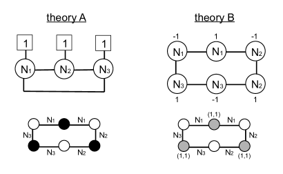
Refer to caption
Figure 15: Pure Chern-Simons theory B is the TTsuperscript𝑇TT^{\rm T}-dual of Yang-Mills theory A.

It should be noticed however that SL(2,)𝑆𝐿2SL(2,\mathbb{Z}) dualities are not sufficient to test mirror symmetry for quivers with nodes of varying ranks. Acting with S𝑆S-duality on a generic YM quiver SCFT, one obtains a brane realization involving D5-branes with different numbers of D3-branes ending on their left and on their right. These brane configurations do not have a simple gauge theory description. To arrive at the mirror dual brane configuration, one has to move the D5-branes along the x3superscript𝑥3x^{3} direction, crossing NS5-branes and making the number of D3-branes vary, until a configuration corresponding to a YM quiver is reached. To be able to check mirror symmetry, it is necessary to understand how the 5-brane moves and the D3-brane creation effect is reproduced in matrix models. We turn now to this question.

4 Mirror symmetry and other dualities involving HW moves

To be able to test mirror symmetry we need to combine the S𝑆S-duality transformation of the matrix models with another type of transformation that corresponds to interchanging the positions of 5-branes in the brane realization. For instance consider the case of the self-mirror T(SU(2))𝑇𝑆𝑈2T(SU(2)) theory, which is 𝒩=4𝒩4\mathcal{N}=4 SQED with two fundamental hypermultiplets. Its brane realization involves a single D3-brane stretched between two NS5-branes and intersecting two D5-branes (figure 16). After S𝑆S-duality the NS5-branes have become D5-branes and the D5-branes have been turned into NS5¯¯NS5\overline{\rm NS5}-branes. However we do not know which SCFT is realized by such a brane configuration. To reach a brane configuration that we understand, one has to move the D5-branes in between the two NS5¯¯NS5\overline{\rm NS5}-branes (figure 16) to recover a brane configuration realizing again T(SU(2))𝑇𝑆𝑈2T(SU(2)). When two 5-branes of different types pass through each other, the number of D3-branes stretched between vary. This is known has the Hanany-Witten effect and it is not supposed to affect the IR theory living on the D3-branes. This is why one can use these 5-brane moves to reach the desired brane configuration, as in the case of the self-mirror T(SU(2))𝑇𝑆𝑈2T(SU(2)).

Refer to caption
Figure 16: On the left is the graph of the T(SU(2))𝑇𝑆𝑈2T(SU(2)) theory, then the the graph resulting from the action of S𝑆S-duality and below is the graph obtained after moving the external D5-branes (black dots) in-between the two NS5-branes (white dots), recovering the graph of T(SU(2))𝑇𝑆𝑈2T(SU(2)), which is a self mirror theory

In this section we show that the 5-brane moves, with brane creation effect, are reproduced by identities in the matrix model, allowing us to prove the equality of partition functions for mirror dual theories with nodes of arbitrary ranks. Moreover these HW-identities can also be used to test various dualities between CS quiver SCFTs involving 5-brane moves. Combined with SL(2,)𝑆𝐿2SL(2,\mathbb{Z}) dualities, they generate a rich web of dualities for 𝒩=4𝒩4\mathcal{N}=4 quiver SCFTs.

4.1 Hanany-Witten moves

Hanany-Witten 5-brane moves refer to the situation when a D5-brane and a NS5-brane pass through each other by moving along the x3superscript𝑥3x^{3} direction. The conservation of 3-form fluxes on the 5-brane worldvolumes implies the creation of a D3-brane stretched between them [4]. In the meantime the D3-branes that were initially stretched between the D5- and NS5-branes have their orientation reversed an become anti-D3-branes, annihilating with other D3-branes. In total we arrive at the following rule: if the initial configuration has a D5-brane with N1subscript𝑁1N_{1} D3-branes ending on its left, a NS5-brane with N3subscript𝑁3N_{3} D3-branes ending on its right and N2subscript𝑁2N_{2} D3-branes are stretched between the two 5-branes, then after the HW move the positions of the 5-branes are exchanged and the number of D3-branes stretched between the two has changed to N~2=N1+N3N2+1subscript~𝑁2subscript𝑁1subscript𝑁3subscript𝑁21\widetilde{N}_{2}=N_{1}+N_{3}-N_{2}+1. This is summarized in the graphs of figure 17-a. The HW 5-brane move has a generalization when one considers the exchange of a (p1,q1)subscript𝑝1subscript𝑞1(p_{1},q_{1})-5brane and a (p2,q2)subscript𝑝2subscript𝑞2(p_{2},q_{2})-5brane, with D=|p1q2p2q1|>0𝐷subscript𝑝1subscript𝑞2subscript𝑝2subscript𝑞10D=|p_{1}q_{2}-p_{2}q_{1}|>0, in which case D𝐷D new D3-branes are created and the final number of D3-branes stretched between the two 5-branes is N~2=N1+N3N2+Dsubscript~𝑁2subscript𝑁1subscript𝑁3subscript𝑁2𝐷\widetilde{N}_{2}=N_{1}+N_{3}-N_{2}+D [33] (see figure 17-b). Note the we do not consider the exchange of 5-branes of the same type, which would have D=0𝐷0D=0, and for which the argument developed in [4] does not apply. These “forbidden” 5-brane moves are related to 𝒩=4𝒩4\mathcal{N}=4 Seiberg-like dualities and involve subtleties that we hope to address in the future.

It is important to notice that the number N2subscript𝑁2N_{2} of D3-branes stretched between a D5-brane and a NS5-brane obeys the constraint N2N1+N3+1subscript𝑁2subscript𝑁1subscript𝑁31N_{2}\leq N_{1}+N_{3}+1 to ensure unbroken supersymmetry. This follows from the “s-rule” ([4, 37]) that says that supersymmetry is broken if more than one D3-branes are stretched between a D5-brane and a NS5-brane. The counterpart for (p1,q1)subscript𝑝1subscript𝑞1(p_{1},q_{1})- and (p2,q2)subscript𝑝2subscript𝑞2(p_{2},q_{2})-5branes is that there must not be more than D𝐷D D3-branes stretched bewteen the two 5branes, leading to N2N1+N3+Dsubscript𝑁2subscript𝑁1subscript𝑁3𝐷N_{2}\leq N_{1}+N_{3}+D. This ensures N~20subscript~𝑁20\widetilde{N}_{2}\geq 0.

Refer to caption
Figure 17: Parts of graphs of two theories related by a Hanany-Witten move. a) A D5-brane (black dot) and a NS5-brane (white dot) are exchanged and the rank of the middle link is changed from N2subscript𝑁2N_{2} to N~2=N1+N3N2+1subscript~𝑁2subscript𝑁1subscript𝑁3subscript𝑁21\widetilde{N}_{2}=N_{1}+N_{3}-N_{2}+1. b) Generic (p1,q1)subscript𝑝1subscript𝑞1(p_{1},q_{1})- and (p2,q2)subscript𝑝2subscript𝑞2(p_{2},q_{2})-5branes are exchanged, with D=|p1q2p2q1|>0𝐷subscript𝑝1subscript𝑞2subscript𝑝2subscript𝑞10D=|p_{1}q_{2}-p_{2}q_{1}|>0. In this case N~2=N1+N3N2+Dsubscript~𝑁2subscript𝑁1subscript𝑁3subscript𝑁2𝐷\widetilde{N}_{2}=N_{1}+N_{3}-N_{2}+D.

The claim of [38] is that the two brane configurations represented by the graphs in figure 17 flow to equivalent IR theories. For the matrix models this imply the following identity for (p1,q1)subscript𝑝1subscript𝑞1(p_{1},q_{1})- and (p2,q2)subscript𝑝2subscript𝑞2(p_{2},q_{2})-5brane factors:

([p1q1][p2q2](N2))σσ~\displaystyle\left({\left[\begin{array}[]{c}p_{1}\\ q_{1}\end{array}\right]}{}_{(N_{2})}{\left[\begin{array}[]{c}p_{2}\\ q_{2}\end{array}\right]}\right)_{\sigma\widetilde{\sigma}} =?([p2q2][p1q1](N~2))σσ~.\displaystyle\stackrel{{\scriptstyle?}}{{=}}\left({\left[\begin{array}[]{c}p_{2}\\ q_{2}\end{array}\right]}{}_{(\widetilde{N}_{2})}{\left[\begin{array}[]{c}p_{1}\\ q_{1}\end{array}\right]}\right)_{\sigma\widetilde{\sigma}}\ . (4.9)

This identity would ensure that the SCFT realized with the (p1,q1)subscript𝑝1subscript𝑞1(p_{1},q_{1})- and (p2,q2)subscript𝑝2subscript𝑞2(p_{2},q_{2})-5branes has the same partition function has the theory realized with the same brane configuration, but with these two 5-branes exchanged. Again we used the symbol =?superscript?\stackrel{{\scriptstyle?}}{{=}} to point out that we have not proven this relation yet and that it will be modified ultimately by the addition of some phase.

The identity (4.9) is difficult to prove, however we can use the local SL(2,)𝑆𝐿2SL(2,\mathbb{Z}) action on matrix models to trade the (p1,q1)subscript𝑝1subscript𝑞1(p_{1},q_{1})-5brane factor and (p2,q2)subscript𝑝2subscript𝑞2(p_{2},q_{2})-5brane factor for a D5-brane factor and a generic (p,q)𝑝𝑞(p,q)-5brane factor with p0𝑝0p\neq 0. The identity to prove is reduced to

([01][pq](N2))σσ~\displaystyle\left({\left[\begin{array}[]{c}0\\ 1\end{array}\right]}{}_{(N_{2})}{\left[\begin{array}[]{c}p\\ q\end{array}\right]}\right)_{\sigma\widetilde{\sigma}} =?([pq][01](N~2))σσ~,\displaystyle\stackrel{{\scriptstyle?}}{{=}}\left({\left[\begin{array}[]{c}p\\ q\end{array}\right]}{}_{(\widetilde{N}_{2})}{\left[\begin{array}[]{c}0\\ 1\end{array}\right]}\right)_{\sigma\widetilde{\sigma}}\ , (4.18)

with N~2=N1+N3N2+|p|subscript~𝑁2subscript𝑁1subscript𝑁3subscript𝑁2𝑝\widetilde{N}_{2}=N_{1}+N_{3}-N_{2}+|p|. Deriving this identity involves various tricks and manipulations that we present in appendix C.2. The computation relies on properties of the special δ^^𝛿\hat{\delta} distributions that enter into the D5-brane matrix factor(3.203) and requires several mathematical identities given in appendix B. Moreover it is necessary to deal with various cases corresponding to different ordering of N1,N2,N3,N1+p,N3+psubscript𝑁1subscript𝑁2subscript𝑁3subscript𝑁1𝑝subscript𝑁3𝑝N_{1},N_{2},N_{3},N_{1}+p,N_{3}+p. In appendix C.2, we discuss only the case N1+pN2N3subscript𝑁1𝑝subscript𝑁2subscript𝑁3N_{1}+p\leq N_{2}\leq N_{3}, which contains the tricks necessary to deal with the other cases. There are however cases for which we were not able to finish the computations due to some additional complications appearing, corresponding to 0<N2<|p|0subscript𝑁2𝑝0<N_{2}<|p| and N1+N3<N2<N1+N3+|p|subscript𝑁1subscript𝑁3brasubscript𝑁2brasubscript𝑁1limit-fromsubscript𝑁3𝑝N_{1}+N_{3}<N_{2}<N_{1}+N_{3}+|p| 141414We believe however that the identities hold also for these cases.. In the dualities that we discuss in this work, we only consider p=±1𝑝plus-or-minus1p=\pm 1 for which these cases do not exist.

Our final result is (C.67) 151515In our computation we have not taken care of overall factors of i𝑖i, so our result is only valid up to factors of i𝑖i. This can be justified by the fact that the partition function is generally complex and that it is not clear wether the initial matrix model summarized in 3.1 contains the correct factors of i𝑖i or not (see [6] for a related discussion).

([01][pq](N2))σσ~\displaystyle\left({\left[\begin{array}[]{c}0\\ 1\end{array}\right]}{}_{(N_{2})}{\left[\begin{array}[]{c}p\\ q\end{array}\right]}\right)_{\sigma\widetilde{\sigma}} =e2πitme±πiqm2eπi12qpΦ([pq][01](N~2))σσ~,\displaystyle=\ e^{\mp 2\pi itm}\ e^{\pm\pi iqm^{2}}\ e^{\frac{\pi i}{12}\frac{q}{p}\Phi}\ \left({\left[\begin{array}[]{c}p\\ q\end{array}\right]}{}_{(\widetilde{N}_{2})}{\left[\begin{array}[]{c}0\\ 1\end{array}\right]}\right)_{\sigma\widetilde{\sigma}}\ , (4.27)

where ±plus-or-minus\pm is the sign of p𝑝p (and minus-or-plus\mp its opposite) and Φ=|Δ21|(Δ2121)|Δ32~|(Δ32~21)ΦsubscriptΔ21superscriptsubscriptΔ2121subscriptΔ3~2superscriptsubscriptΔ3~221\Phi=|\Delta_{21}|(\Delta_{21}^{2}-1)-|\Delta_{3\widetilde{2}}|(\Delta_{3\widetilde{2}}^{2}-1), with Δ21=N2N1subscriptΔ21subscript𝑁2subscript𝑁1\Delta_{21}=N_{2}-N_{1} and Δ32~=N3N~2subscriptΔ3~2subscript𝑁3subscript~𝑁2\Delta_{3\widetilde{2}}=N_{3}-\widetilde{N}_{2}. The extra phase in the relation (4.27) contains matrix factors for a background CS term with level ±qplus-or-minus𝑞\pm q for the U(1)𝑈1U(1) global symmetry associated to m𝑚m and a background BF coupling between the two U(1)𝑈1U(1) global symmetries associated to m𝑚m and t𝑡t, which can be viewed as a mixed CS coupling with level 1minus-or-plus1\mp 1. The CS levels are integers, implying that such background terms do not affect the physics of the theory [28].

We are now in a position to argue for the equality of the partition functions, up to irrelevant phases, of mirror dual theories for YM quiver SCFTs with nodes of arbitrary ranks.

4.2 Mirror symmetry

Mirror symmetry is a duality that relates pairs of 𝒩=4𝒩4\mathcal{N}=4 Yang-Mills quiver SCFTs, satisfying the “good” conditions of [23], namely at each node Mj+Nj+1+Nj12Njsubscript𝑀𝑗subscript𝑁𝑗1subscript𝑁𝑗12subscript𝑁𝑗M_{j}+N_{j+1}+N_{j-1}\geq 2N_{j}, where Mjsubscript𝑀𝑗M_{j} is the number of fundamental hypermultiplets of the node U(Nj)𝑈subscript𝑁𝑗U(N_{j}). The mirror dual of a YM quiver theory A is found by first considering the brane configuration realizing A, with D5 and NS5-branes, then taking the S𝑆S-dual of this brane configuration and implementing HW moves until the D5-branes have the same number of D3-branes on each side. One obtains the brane configuration realizing a YM quiver theory B, which is the mirror dual of the theory A. For this algorithm to work, it is necessary that, after some HW moves, each D5-brane arrives at a position where it has zero net number of D3-branes ending on it, where by net number we mean the number of D3-branes ending on its right, minus the number of D3-branes ending on its left. Although it is not completely straightforward, this is ensured by the conditions Mj+Nj+1+Nj12Njsubscript𝑀𝑗subscript𝑁𝑗1subscript𝑁𝑗12subscript𝑁𝑗M_{j}+N_{j+1}+N_{j-1}\geq 2N_{j} that define a “good” quiver. Note also that the mirror theory B is also a “good” quiver theory.

The partition functions of mirror dual theories A and B can be mapped using the tools we have developed. The partition function ZAsubscript𝑍𝐴Z_{A} of the theory A is given by the sequence of 5-brane factors mimicking its brane realization, for instance:

ZAsubscript𝑍𝐴\displaystyle Z_{A} =Tr[10][01](N1)[01](N1)[10](N1)[01](N2)[10](N2)(N3)[01](NP^).(NP^)\displaystyle=\textrm{Tr}\ {\left[\begin{array}[]{c}1\\ 0\end{array}\right]}{}_{(N_{1})}{\left[\begin{array}[]{c}0\\ 1\end{array}\right]}{}_{(N_{1})}{\left[\begin{array}[]{c}0\\ 1\end{array}\right]}{}_{(N_{1})}{\left[\begin{array}[]{c}1\\ 0\end{array}\right]}{}_{(N_{2})}{\left[\begin{array}[]{c}0\\ 1\end{array}\right]}{}_{(N_{2})}{\left[\begin{array}[]{c}1\\ 0\end{array}\right]}{}_{(N_{3})}\cdots{}_{(N_{\widehat{P}})}{\left[\begin{array}[]{c}0\\ 1\end{array}\right]}{}_{(N_{\widehat{P}})}\ . (4.42)

Each 5-brane factor can be replaced by its local S𝑆S-dual using (3.237):

ZAsubscript𝑍𝐴\displaystyle Z_{A} =TrS1[01]SS1[10]SS1[10]SS1[01]SS1[10]SS1[10]SabsentTrsuperscript𝑆1delimited-[]01𝑆superscript𝑆1delimited-[]10𝑆superscript𝑆1delimited-[]10𝑆superscript𝑆1delimited-[]01𝑆superscript𝑆1delimited-[]10𝑆superscript𝑆1delimited-[]10𝑆\displaystyle=\textrm{Tr}\ S^{-1}{\left[\begin{array}[]{c}0\\ 1\end{array}\right]}S\,S^{-1}{\left[\begin{array}[]{c}-1\\ 0\end{array}\right]}S\,S^{-1}{\left[\begin{array}[]{c}-1\\ 0\end{array}\right]}S\,S^{-1}{\left[\begin{array}[]{c}0\\ 1\end{array}\right]}S\,S^{-1}{\left[\begin{array}[]{c}-1\\ 0\end{array}\right]}S\,\cdots\,S^{-1}{\left[\begin{array}[]{c}-1\\ 0\end{array}\right]}S (4.55)
=Tr[01][10](N1)[10](N1)[01](N1)[10](N2)[01](N2)(N3)[10](NP^),(NP^)\displaystyle=\textrm{Tr}\ {\left[\begin{array}[]{c}0\\ 1\end{array}\right]}{}_{(N_{1})}{\left[\begin{array}[]{c}-1\\ 0\end{array}\right]}{}_{(N_{1})}{\left[\begin{array}[]{c}-1\\ 0\end{array}\right]}{}_{(N_{1})}{\left[\begin{array}[]{c}0\\ 1\end{array}\right]}{}_{(N_{2})}{\left[\begin{array}[]{c}-1\\ 0\end{array}\right]}{}_{(N_{2})}{\left[\begin{array}[]{c}0\\ 1\end{array}\right]}{}_{(N_{3})}\cdots{}_{(N_{\widehat{P}})}{\left[\begin{array}[]{c}-1\\ 0\end{array}\right]}{}_{(N_{\widehat{P}})}\ , (4.70)

At this stage the matrix model is given by the sequence of D5 and NS5¯¯NS5\overline{\rm NS5} factors, but the associated brane configuration has D5-branes with different numbers of D3-branes on each side (except when all Nisubscript𝑁𝑖N_{i} are equal). Then we can use the identity (4.27) to exchange D5- and NS5¯¯NS5\overline{\rm NS5} factors. For instance if N1>NP^(N0)subscript𝑁1annotatedsubscript𝑁^𝑃absentsubscript𝑁0N_{1}>N_{\hat{P}}\,(\equiv N_{0}), we have to exchange the two first factors:

ZAsubscript𝑍𝐴\displaystyle Z_{A} =eiφTr[10][01](N~1)[10](N1)[01](N1)(N2)[10](NP^),(NP^)\displaystyle=\ e^{i\varphi}\ \textrm{Tr}\ {\left[\begin{array}[]{c}-1\\ 0\end{array}\right]}{}_{(\widetilde{N}_{1})}{\left[\begin{array}[]{c}0\\ 1\end{array}\right]}{}_{(N_{1})}{\left[\begin{array}[]{c}-1\\ 0\end{array}\right]}{}_{(N_{1})}{\left[\begin{array}[]{c}0\\ 1\end{array}\right]}{}_{(N_{2})}\cdots{}_{(N_{\widehat{P}})}{\left[\begin{array}[]{c}-1\\ 0\end{array}\right]}{}_{(N_{\widehat{P}})}\ , (4.82)

where N~1=N1+NP^N1+1=NP^+1subscript~𝑁1subscript𝑁1subscript𝑁^𝑃subscript𝑁11subscript𝑁^𝑃1\widetilde{N}_{1}=N_{1}+N_{\hat{P}}-N_{1}+1=N_{\hat{P}}+1 and eiφsuperscript𝑒𝑖𝜑e^{i\varphi} is a phase depending on the background parameters. Note that the net number of D3-branes ending on the D5-brane has decreased by one unit. If N~1<N1subscript~𝑁1subscript𝑁1\widetilde{N}_{1}<N_{1}, we have to continue moving the same D5-factor to the right of the chain of factors by permuting with NS5¯¯NS5\overline{\rm NS5} factors, until the net number of D3-branes ending on it is zero (it decreases by one unit at each permutation). The fact that there are enough NS5¯¯NS5\overline{\rm NS5} factors is ensured by the conditions defining a “good” quiver. The same algorithm must be applied to all D5-factors, so that in the end they all have zero net number of D3-branes ending on them.

ZAsubscript𝑍𝐴\displaystyle Z_{A} =eiφABTr[10](N~1)=(NP^)eiϕABZB.\displaystyle=e^{i\varphi_{AB}}\ \textrm{Tr}\ {\left[\begin{array}[]{c}-1\\ 0\end{array}\right]}{}_{(\widetilde{N}_{1})}\ \cdots\ {}_{(N_{\widehat{P}})}\ =\ e^{i\phi_{AB}}\ Z_{B}\ . (4.86)

The final sequence of D5 and NS5¯¯NS5\overline{\rm NS5} factors is obviously very different from the initial sequence associated to the theory A, instead it corresponds precisely to the sequence associated to the brane configuration of theory B. This is because the permutations of 5-brane factors reproduce exactly the HW 5-brane moves that are needed to go to the brane configuration realizing the mirror theory B.

As discussed in section 3.4, it is common to complete the transformation of the brane configuration by a “rotation” that changes the NS5¯¯NS5\overline{\rm NS5}-branes into NS5-branes. At the level of the matrix model, this corresponds to reversing the sequence of 5-brane factors and trading the NS5¯¯NS5\overline{\rm NS5} factors for NS5-factors. This is actually a simple relabelling of the eigenvalues (from right to left) that does not affect the matrix model.

In the end we find that the partition functions ZAsubscript𝑍𝐴Z_{A} and ZBsubscript𝑍𝐵Z_{B} differ only by a phase eiφABsuperscript𝑒𝑖subscript𝜑𝐴𝐵e^{i\varphi_{AB}}, corresponding to unphysical background CS terms. If {mi,tj}subscript𝑚𝑖subscript𝑡𝑗\{m_{i},t_{j}\}, 1iP1𝑖𝑃1\leq i\leq P, 1jP^1𝑗^𝑃1\leq j\leq\hat{P}, are the mass and FI deformation parameters of theory A, then deformation parameters of theory B are the FI parameters t^i=misubscript^𝑡𝑖subscript𝑚𝑖\hat{t}_{i}=m_{i} and the mass parameters m^j=tjsubscript^𝑚𝑗subscript𝑡𝑗\hat{m}_{j}=t_{j}.

The map between the exact partition functions of the SCFTs A and B, with FI and mass deformation terms, provides a important new test of mirror symmetry for all non-abelian circular and linear161616The test for linear quivers corresponds to having NP^=0subscript𝑁^𝑃0N_{\widehat{P}}=0 in the above argument. YM quiver SCFTs.

4.3 Level-rank and YM-CS dualities

The identity (4.27) can be used to test other dualities that involve 5-brane moves. Such dualities have already been described for a few abelian SCFTs in [17]. Instead of trying to describe all possible dualities, we will concentrate on specific interesting cases corresponding to 𝒩=4𝒩4\mathcal{N}=4 level-rank dualities for CS quiver theories and dualities mapping YM quiver SCFTs and pure Chern-Simons SCFTs.

CS quiver theories are realized with brane configurations corresponding sequences of NS5-branes and (1,k)1𝑘(1,k)-5branes (see section 2.2). Permuting a NS5-brane and a (1,k)1𝑘(1,k)-5brane, adjacent in a brane sequence, leads to the brane configuration of a dual CS quiver theory, as illustrated in figure 18. The 5-brane exchange affects three consecutive gauge nodes of the quiver, in particular the central node is changed from U(N2)k𝑈subscriptsubscript𝑁2𝑘U(N_{2})_{k} to U(N~2)k𝑈subscriptsubscript~𝑁2𝑘U(\widetilde{N}_{2})_{-k} with N~2=N1+N3N2+|k|subscript~𝑁2subscript𝑁1subscript𝑁3subscript𝑁2𝑘\widetilde{N}_{2}=N_{1}+N_{3}-N_{2}+|k|. This can be seen as a generalization to 𝒩=4𝒩4\mathcal{N}=4 quiver SCFTs of the Giveon-Kutasov duality for 𝒩=2𝒩2\mathcal{N}=2 SCFTs [39] (tests of the Giveon-Kutasov duality using exact partition functions were presented in [40]), which is already a generalization of the level-rank duality of simple Chern-Simons theory without matter.
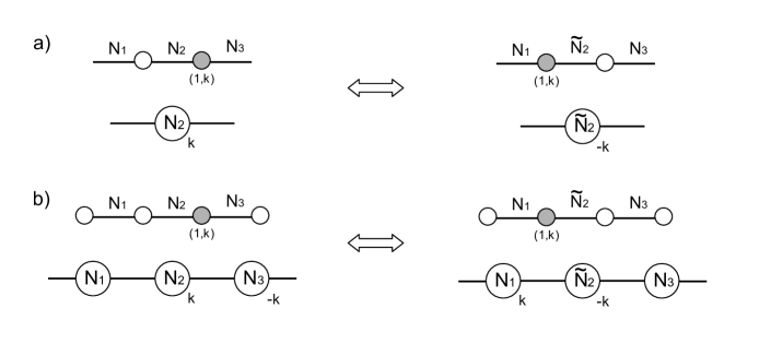
Refer to caption
Figure 18: a) A HW-move in CS quiver theories. The rank and CS level of the central node are changed for N~2=N1+N3N2+|k|subscript~𝑁2subscript𝑁1subscript𝑁3subscript𝑁2𝑘\widetilde{N}_{2}=N_{1}+N_{3}-N_{2}+|k| and k𝑘-k. b) Example of dual theories obtained from a single HW move. Only the element of the quivers changing under the duality are shown, the rest of the quiver is identical for the two theories.

The equality of matrix models of the two dual theories, up to a phase, is ensured by the HW relation:

[10](N1)[1k](N2)(N3)\displaystyle{}_{(N_{1})}{\left[\begin{array}[]{c}1\\ 0\end{array}\right]}{}_{(N_{2})}{\left[\begin{array}[]{c}1\\ k\end{array}\right]}{}_{(N_{3})} =eπi(ts)2[1k](N1)[10](N~2),(N3)\displaystyle=\ e^{-\pi i\,(t-s)^{2}}\ {}_{(N_{1})}{\left[\begin{array}[]{c}1\\ k\end{array}\right]}{}_{(\widetilde{N}_{2})}{\left[\begin{array}[]{c}1\\ 0\end{array}\right]}{}_{(N_{3})}\ , (4.96)

which is obtained using (3.178), (3.237) and  (4.27) in the following way: 171717we omit here the phases of the form eiπ12()superscript𝑒𝑖𝜋12e^{\frac{i\pi}{12}(...)} that are independent of the parameters of the theory and play no role in the derivation of the dualities.

[10](N1)[1k](N2)(N3)\displaystyle{}_{(N_{1})}{\left[\begin{array}[]{c}1\\ 0\end{array}\right]}{}_{(N_{2})}{\left[\begin{array}[]{c}1\\ k\end{array}\right]}{}_{(N_{3})} =eπikΔ23s2S1[01][k1](N2)S\displaystyle=\ e^{\frac{\pi i}{k}\Delta_{23}\,s^{2}}\ S^{-1}{\left[\begin{array}[]{c}0\\ 1\end{array}\right]}{}_{(N_{2})}{\left[\begin{array}[]{c}-k\\ 1\end{array}\right]}S
=eπikΔ23s2e2πitseπit2S1[k1][01](N~2)S\displaystyle=\ e^{\frac{\pi i}{k}\Delta_{23}\,s^{2}}\ e^{2\pi i\,ts}\ e^{-\pi i\,t^{2}}\ S^{-1}{\left[\begin{array}[]{c}-k\\ 1\end{array}\right]}{}_{(\widetilde{N}_{2})}{\left[\begin{array}[]{c}0\\ 1\end{array}\right]}S
=eπis2e2πitseπit2[1k](N1)[10](N~2),(N3)\displaystyle=\ e^{-\pi i\,s^{2}}\ e^{2\pi i\,ts}\ e^{-\pi i\,t^{2}}\ {}_{(N_{1})}{\left[\begin{array}[]{c}1\\ k\end{array}\right]}{}_{(\widetilde{N}_{2})}{\left[\begin{array}[]{c}1\\ 0\end{array}\right]}{}_{(N_{3})}\ ,

where t𝑡t and s𝑠s are the deformation parameters associated to the NS5 and (1,k)1𝑘(1,k)-5brane respectively and we have used Δ23Δ12~=ksubscriptΔ23subscriptΔ1~2𝑘\Delta_{23}-\Delta_{1\widetilde{2}}=k. Note that again the extra phase in (4.96) appears as a background CS term with integer level, that does not affect our conclusions regarding dualities. The map between parameters of the dual theories indicates that the FI parameter of the middle node is reversed η2=tsη~2=st=η2subscript𝜂2𝑡𝑠subscript~𝜂2𝑠𝑡subscript𝜂2\eta_{2}=t-s\ \rightarrow\widetilde{\eta}_{2}=s-t=-\eta_{2}. The FI parameters of the two exterior nodes U(N1)𝑈subscript𝑁1U(N_{1}) and U(N3)𝑈subscript𝑁3U(N_{3}) are also affected.

This simple 5-brane permutation can be repeated for all couple of adjacent NS5 and (1,k)1𝑘(1,k)-5brane, leading to a web of dualities between CS quiver SCFTs. The identity (4.96) proves that the exact partition functions of the theories related by these HW-moves are equal, up to an irrelevant phases.


The dualities following from HW 5brane moves can be combined with the SL(2,)𝑆𝐿2SL(2,\mathbb{Z}) dualities to generate interesting dualities. Mirror symmetry between YM SCFTs is one example of such combined dualities. Another interesting case would be a duality mapping Yang-Mills SCFTs to pure Chern-Simons SCFTs, where by pure Chern-Simons we mean that all nodes of the CS quiver have non-vanishing CS levels. The Chern-Simons theories have superconformal Lagrangians and would be understood as an explicit description of the infrared fixed points of the “dual” Yang-Mills quiver theories.

We have already seen in section 3.4 that YM theories have CS duals related through TTsuperscript𝑇TT^{\rm T}-duality, which changes D5-branes into (1,1)11(1,1)-5-branes. However, the CS duals have generically U(N)0𝑈subscript𝑁0U(N)_{0} auxiliary nodes. To obtain a pure CS dual theory we can try to use HW-moves. The necessary and sufficient condition to obtain a pure CS dual theory is that the number of D5-branes and NS5-branes in the brane realization of the initial YM theory are equal for circular quivers, or differ by at most one for linear quivers. In this case, the (1,1)11(1,1)-5branes of the TTsuperscript𝑇TT^{\rm T}-dual CS theory can be moved along the x3superscript𝑥3x^{3} direction to reach a sequence of alternating NS5 and (1,1)11(1,1)-5branes. The corresponding SCFT is then a pure CS theory with alternating Chern-Simons levels ±1plus-or-minus1\pm 1.

The T(SU(N))𝑇𝑆𝑈𝑁T(SU(N)) theories belong to this class of YM theories with pure CS duals. Let us see how the duality works by transforming the partition function of T(SU(4))𝑇𝑆𝑈4T(SU(4)) to its Chern-Simons dual. The partition function of T(SU(4))𝑇𝑆𝑈4T(SU(4)) with deformation parameters t1,2,3,4,m1,2,3,4subscript𝑡1234subscript𝑚1234t_{1,2,3,4},m_{1,2,3,4} is given by the sequence of 5brane factors:

ZT(SU(4))superscript𝑍𝑇𝑆𝑈4\displaystyle Z^{T(SU(4))} =[10][10](1)[10](2)[01](3)[01](3)[01](3)[01](3)[10](3).\displaystyle={\left[\begin{array}[]{c}1\\ 0\end{array}\right]}{}_{(1)}{\left[\begin{array}[]{c}1\\ 0\end{array}\right]}{}_{(2)}{\left[\begin{array}[]{c}1\\ 0\end{array}\right]}{}_{(3)}{\left[\begin{array}[]{c}0\\ 1\end{array}\right]}{}_{(3)}{\left[\begin{array}[]{c}0\\ 1\end{array}\right]}{}_{(3)}{\left[\begin{array}[]{c}0\\ 1\end{array}\right]}{}_{(3)}{\left[\begin{array}[]{c}0\\ 1\end{array}\right]}{}_{(3)}{\left[\begin{array}[]{c}1\\ 0\end{array}\right]}\ . (4.113)

After acting (locally on each 5-brane factor) with TTsuperscript𝑇TT^{\rm T}-duality, the matrix model becomes

ZT(SU(4))superscript𝑍𝑇𝑆𝑈4\displaystyle Z^{T(SU(4))} =eπi(t12+t22+t323t42)[10][10](1)[10](2)[11](3)[11](3)[11](3)[11](3)[10](3),\displaystyle=e^{\pi i(t_{1}^{2}+t_{2}^{2}+t_{3}^{2}-3\,t_{4}^{2})}\ {\left[\begin{array}[]{c}1\\ 0\end{array}\right]}{}_{(1)}{\left[\begin{array}[]{c}1\\ 0\end{array}\right]}{}_{(2)}{\left[\begin{array}[]{c}1\\ 0\end{array}\right]}{}_{(3)}{\left[\begin{array}[]{c}1\\ 1\end{array}\right]}{}_{(3)}{\left[\begin{array}[]{c}1\\ 1\end{array}\right]}{}_{(3)}{\left[\begin{array}[]{c}1\\ 1\end{array}\right]}{}_{(3)}{\left[\begin{array}[]{c}1\\ 1\end{array}\right]}{}_{(3)}{\left[\begin{array}[]{c}1\\ 0\end{array}\right]}\ , (4.130)

where the extra phase is derived from the identities (3.237) and the decomposition TT=TSTsuperscript𝑇T𝑇𝑆𝑇T^{\rm T}=-TST. Next we use the identity (4.96) to rearrange the sequence of factors, so that NS5 and (1,1)11(1,1)-5brane factors alternate:

ZT(SU(4))superscript𝑍𝑇𝑆𝑈4\displaystyle Z^{T(SU(4))} =eπiφ[10][11](1)[10](3)[11](3)[10](4)[11](3)[10](3)[11](1)=ZCS,\displaystyle=e^{\pi i\,\varphi}\ {\left[\begin{array}[]{c}1\\ 0\end{array}\right]}{}_{(1)}{\left[\begin{array}[]{c}1\\ 1\end{array}\right]}{}_{(3)}{\left[\begin{array}[]{c}1\\ 0\end{array}\right]}{}_{(3)}{\left[\begin{array}[]{c}1\\ 1\end{array}\right]}{}_{(4)}{\left[\begin{array}[]{c}1\\ 0\end{array}\right]}{}_{(3)}{\left[\begin{array}[]{c}1\\ 1\end{array}\right]}{}_{(3)}{\left[\begin{array}[]{c}1\\ 0\end{array}\right]}{}_{(1)}{\left[\begin{array}[]{c}1\\ 1\end{array}\right]}\ =\ Z_{\rm CS}, (4.147)

with φ=t12+t22+t323t42(t2m1)2(t3m1)2(t3m2)2+(t4m4)2𝜑superscriptsubscript𝑡12superscriptsubscript𝑡22superscriptsubscript𝑡323superscriptsubscript𝑡42superscriptsubscript𝑡2subscript𝑚12superscriptsubscript𝑡3subscript𝑚12superscriptsubscript𝑡3subscript𝑚22superscriptsubscript𝑡4subscript𝑚42\varphi=t_{1}^{2}+t_{2}^{2}+t_{3}^{2}-3\,t_{4}^{2}-(t_{2}-m_{1})^{2}-(t_{3}-m_{1})^{2}-(t_{3}-m_{2})^{2}+(t_{4}-m_{4})^{2}. The final matrix model correspond to a pure Chern-Simons theory with gauge group U(1)1×U(3)1×U(3)1×U(4)1×U(3)1×U(3)1×U(1)1𝑈subscript11𝑈subscript31𝑈subscript31𝑈subscript41𝑈subscript31𝑈subscript31𝑈subscript11U(1)_{1}\times U(3)_{-1}\times U(3)_{1}\times U(4)_{-1}\times U(3)_{1}\times U(3)_{-1}\times U(1)_{1}. The transformation is summarized in figure 19.
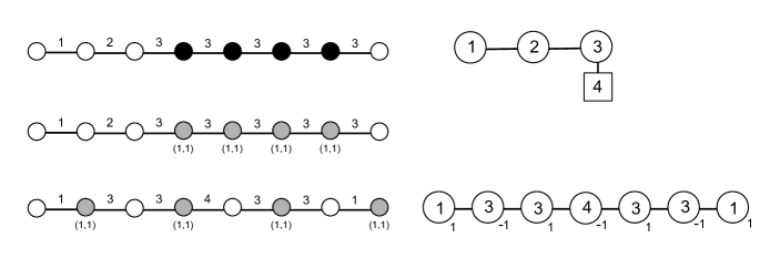
Refer to caption
Figure 19: From top to bottom: quiver and graph of T(SU(4))𝑇𝑆𝑈4T(SU(4)) theory; graph after TTsuperscript𝑇TT^{\rm T} action; graph and quiver of the pure CS dual theory, obtained after HW moves.

The necessary and sufficient condition for a YM fixed point to admit a pure CS description boils down to having a number of nodes equal to the number of fundamental hypermultiplets for circular quivers (or different by at most one for linear quivers). It must also be noticed that the pure Chern-Simons duals of Yang-Mills theories have only nodes with Chern levels ±1plus-or-minus1\pm 1 and thus are never weakly coupled, since the effective gauge coupling in Chern-Simons theory is λ=Nk𝜆𝑁𝑘\lambda=\frac{N}{k} and it can become small only in the large k𝑘k limit.

4.3.1 A check by direct computations

In the argumentation that we have developed, we were able to map partition functions of dual theories without explicitly computing the matrix models. We would like to provide some consistency check of our results by computing matrix models of simple dual theories. Let us consider the three dual abelian theories:

  • T(SU(2))𝑇𝑆𝑈2T(SU(2)), which is a Yang-Mills theory with gauge group U(1)𝑈1U(1) and two fundamental hypermultiplets. The deformation parameters are the FI parameter t1t2subscript𝑡1subscript𝑡2t_{1}-t_{2} and the real masses m1,m2subscript𝑚1subscript𝑚2m_{1},m_{2}. We denote its partition function ZAsubscript𝑍𝐴Z_{A};

  • the CS theory with gauge group U(1)1×U(1)0×U(1)1𝑈subscript11𝑈subscript10𝑈subscript11U(1)_{1}\times U(1)_{0}\times U(1)_{-1}, with FI parameters t^1t^2,t^2t^3,t^3t^4subscript^𝑡1subscript^𝑡2subscript^𝑡2subscript^𝑡3subscript^𝑡3subscript^𝑡4\hat{t}_{1}-\hat{t}_{2},\hat{t}_{2}-\hat{t}_{3},\hat{t}_{3}-\hat{t}_{4}. We denote its partition function ZBsubscript𝑍𝐵Z_{B};

  • the pure CS theory with gauge group U(1)1×U(1)1×U(1)1𝑈subscript11𝑈subscript11𝑈subscript11U(1)_{1}\times U(1)_{-1}\times U(1)_{1}, with FI parameters tˇ1tˇ2,tˇ2tˇ3,tˇ3tˇ4subscriptˇ𝑡1subscriptˇ𝑡2subscriptˇ𝑡2subscriptˇ𝑡3subscriptˇ𝑡3subscriptˇ𝑡4\check{t}_{1}-\check{t}_{2},\check{t}_{2}-\check{t}_{3},\check{t}_{3}-\check{t}_{4}. We denote its partition function ZCsubscript𝑍𝐶Z_{C}.

These abelian duals were already proposed in [17], where it was shown that their moduli spaces coincide. In addition our analysis provides the following map between parameters

t1subscript𝑡1\displaystyle t_{1} =t^1=tˇ1,m1=t^2=tˇ2,m2=t^3=tˇ4,t2=t^4=tˇ3.\displaystyle=\ \hat{t}_{1}\ =\ \check{t}_{1}\quad,\quad m_{1}=\ \hat{t}_{2}\ =\ \check{t}_{2}\quad,\quad m_{2}\ =\ \hat{t}_{3}\ =\ \check{t}_{4}\quad,\quad t_{2}=\ \hat{t}_{4}\ =\ \check{t}_{3}\ . (4.148)

The gauge quivers and corresponding graphs are presented in figure 20. The theories A and B be are related by TTsuperscript𝑇TT^{\rm T}-duality, while the theories B and C are related by a HW move or level-rank duality.

Refer to caption
Figure 20: Quivers and graphs of three abelian dual theories.

The map between partition functions obtained by acting with TTsuperscript𝑇TT^{\rm T} duality on the matrix model, using (3.178,3.237), is given by:

ZA=eiπ(t12t22)ZB=eiπ[t12t22+(t2m2)2]ZC,subscript𝑍𝐴superscript𝑒𝑖𝜋superscriptsubscript𝑡12superscriptsubscript𝑡22subscript𝑍𝐵superscript𝑒𝑖𝜋delimited-[]superscriptsubscript𝑡12superscriptsubscript𝑡22superscriptsubscript𝑡2subscript𝑚22subscript𝑍𝐶\displaystyle Z_{A}=e^{i\pi(t_{1}^{2}-t_{2}^{2})}\,Z_{B}=e^{i\pi[t_{1}^{2}-t_{2}^{2}+(t_{2}-m_{2})^{2}]}\,Z_{C}\ , (4.149)

up to overall phases independent of the deformation parameters.

The matrix model for the T(SU(2))𝑇𝑆𝑈2T(SU(2)) theory is given by:

ZAsubscript𝑍𝐴\displaystyle Z_{A} =ZT(SU(2))=𝑑σe2πi(t1t2)σch(σm1)ch(σm2)=(i)e2πi(t1t2)m1e2πi(t1t2)m2sh(t1t2)sh(m1m2),absentsuperscript𝑍𝑇𝑆𝑈2differential-d𝜎superscript𝑒2𝜋𝑖subscript𝑡1subscript𝑡2𝜎ch𝜎subscript𝑚1ch𝜎subscript𝑚2𝑖superscript𝑒2𝜋𝑖subscript𝑡1subscript𝑡2subscript𝑚1superscript𝑒2𝜋𝑖subscript𝑡1subscript𝑡2subscript𝑚2shsubscript𝑡1subscript𝑡2shsubscript𝑚1subscript𝑚2\displaystyle=\ Z^{T(SU(2))}\ =\ \int d\sigma\ \frac{e^{2\pi i(t_{1}-t_{2})\sigma}}{\textrm{ch}(\sigma-m_{1})\textrm{ch}(\sigma-m_{2})}\ =\ (-i)\,\frac{e^{2\pi i(t_{1}-t_{2})m_{1}}-e^{2\pi i(t_{1}-t_{2})m_{2}}}{\textrm{sh}(t_{1}-t_{2})\textrm{sh}(m_{1}-m_{2})}\ ,

where the integral was computed by deforming the contour to i𝑖i\,\infty and summing over residues. The partition function for the CS theory B is given by:

ZBsubscript𝑍𝐵\displaystyle Z_{B} =𝑑σ1𝑑σ2𝑑σ3eπi(σ12σ32)e2πi[(t^1t^2)σ1+(t^2t^3)σ2+(t^3t^4)σ3]ch(σ1σ2)ch(σ2σ3).absentdifferential-dsubscript𝜎1differential-dsubscript𝜎2differential-dsubscript𝜎3superscript𝑒𝜋𝑖superscriptsubscript𝜎12superscriptsubscript𝜎32superscript𝑒2𝜋𝑖delimited-[]subscript^𝑡1subscript^𝑡2subscript𝜎1subscript^𝑡2subscript^𝑡3subscript𝜎2subscript^𝑡3subscript^𝑡4subscript𝜎3chsubscript𝜎1subscript𝜎2chsubscript𝜎2subscript𝜎3\displaystyle=\ \int d\sigma_{1}d\sigma_{2}d\sigma_{3}\ e^{\pi i(\sigma_{1}^{2}-\sigma_{3}^{2})}\ \frac{e^{2\pi i[(\hat{t}_{1}-\hat{t}_{2})\sigma_{1}+(\hat{t}_{2}-\hat{t}_{3})\sigma_{2}+(\hat{t}_{3}-\hat{t}_{4})\sigma_{3}]}}{\textrm{ch}(\sigma_{1}-\sigma_{2})\textrm{ch}(\sigma_{2}-\sigma_{3})}\ .

To evaluate these integrals, we change variables σ1σ1+σ2subscript𝜎1subscript𝜎1subscript𝜎2\sigma_{1}\rightarrow\sigma_{1}+\sigma_{2}, σ3σ3+σ2subscript𝜎3subscript𝜎3subscript𝜎2\sigma_{3}\rightarrow\sigma_{3}+\sigma_{2} . Then the integration over σ2subscript𝜎2\sigma_{2} yields a delta function that can be used to integrate over σ1subscript𝜎1\sigma_{1}, leading to

ZBsubscript𝑍𝐵\displaystyle Z_{B} =eπi(t^42t^12)e2πi(t^1t^4)t^2𝑑σ3e2πi(t^3t^2)σ3ch(σ3t^1+t^4)ch(σ3)absentsuperscript𝑒𝜋𝑖superscriptsubscript^𝑡42superscriptsubscript^𝑡12superscript𝑒2𝜋𝑖subscript^𝑡1subscript^𝑡4subscript^𝑡2differential-dsubscript𝜎3superscript𝑒2𝜋𝑖subscript^𝑡3subscript^𝑡2subscript𝜎3chsubscript𝜎3subscript^𝑡1subscript^𝑡4chsubscript𝜎3\displaystyle=\ e^{\pi i(\hat{t}_{4}^{2}-\hat{t}_{1}^{2})}\ e^{2\pi i(\hat{t}_{1}-\hat{t}_{4})\hat{t}_{2}}\int d\sigma_{3}\ \frac{e^{2\pi i(\hat{t}_{3}-\hat{t}_{2})\sigma_{3}}}{\textrm{ch}(\sigma_{3}-\hat{t}_{1}+\hat{t}_{4})\textrm{ch}(\sigma_{3})}
=eπi(t^42t^12)(i)e2πi(t^1t^4)t^2e2πi(t^1t^4)t^3sh(t^1t^4)sh(t^2t^3).absentsuperscript𝑒𝜋𝑖superscriptsubscript^𝑡42superscriptsubscript^𝑡12𝑖superscript𝑒2𝜋𝑖subscript^𝑡1subscript^𝑡4subscript^𝑡2superscript𝑒2𝜋𝑖subscript^𝑡1subscript^𝑡4subscript^𝑡3shsubscript^𝑡1subscript^𝑡4shsubscript^𝑡2subscript^𝑡3\displaystyle=\ e^{\pi i(\hat{t}_{4}^{2}-\hat{t}_{1}^{2})}\ (-i)\,\frac{e^{2\pi i(\hat{t}_{1}-\hat{t}_{4})\hat{t}_{2}}-e^{2\pi i(\hat{t}_{1}-\hat{t}_{4})\hat{t}_{3}}}{\textrm{sh}(\hat{t}_{1}-\hat{t}_{4})\textrm{sh}(\hat{t}_{2}-\hat{t}_{3})}\ .

The partition function of the pure Chern-Simons theory C can be evaluated using similar ideas, giving

ZCsubscript𝑍𝐶\displaystyle Z_{C} =𝑑σ1𝑑σ2𝑑σ3eπi(σ12σ22+σ32)e2πi[(tˇ1tˇ2)σ1+(tˇ2tˇ3)σ2+(tˇ3tˇ4)σ3]ch(σ1σ2)ch(σ2σ3)absentdifferential-dsubscript𝜎1differential-dsubscript𝜎2differential-dsubscript𝜎3superscript𝑒𝜋𝑖superscriptsubscript𝜎12superscriptsubscript𝜎22superscriptsubscript𝜎32superscript𝑒2𝜋𝑖delimited-[]subscriptˇ𝑡1subscriptˇ𝑡2subscript𝜎1subscriptˇ𝑡2subscriptˇ𝑡3subscript𝜎2subscriptˇ𝑡3subscriptˇ𝑡4subscript𝜎3chsubscript𝜎1subscript𝜎2chsubscript𝜎2subscript𝜎3\displaystyle=\ \int d\sigma_{1}d\sigma_{2}d\sigma_{3}\ e^{\pi i(\sigma_{1}^{2}-\sigma_{2}^{2}+\sigma_{3}^{2})}\,\frac{e^{2\pi i[(\check{t}_{1}-\check{t}_{2})\sigma_{1}+(\check{t}_{2}-\check{t}_{3})\sigma_{2}+(\check{t}_{3}-\check{t}_{4})\sigma_{3}]}}{\textrm{ch}(\sigma_{1}-\sigma_{2})\textrm{ch}(\sigma_{2}-\sigma_{3})}
=eπi4eπi(tˇ12+tˇ422tˇ3tˇ4)(i)e2πi(tˇ1tˇ3)tˇ2e2πi(tˇ1tˇ3)tˇ4sh(tˇ1tˇ3)sh(tˇ2tˇ4).absentsuperscript𝑒𝜋𝑖4superscript𝑒𝜋𝑖superscriptsubscriptˇ𝑡12superscriptsubscriptˇ𝑡422subscriptˇ𝑡3subscriptˇ𝑡4𝑖superscript𝑒2𝜋𝑖subscriptˇ𝑡1subscriptˇ𝑡3subscriptˇ𝑡2superscript𝑒2𝜋𝑖subscriptˇ𝑡1subscriptˇ𝑡3subscriptˇ𝑡4shsubscriptˇ𝑡1subscriptˇ𝑡3shsubscriptˇ𝑡2subscriptˇ𝑡4\displaystyle\ =\ e^{-\frac{\pi i}{4}}\ e^{-\pi i(\check{t}_{1}^{2}+\check{t}_{4}^{2}-2\check{t}_{3}\check{t}_{4})}\ (-i)\,\frac{e^{2\pi i(\check{t}_{1}-\check{t}_{3})\check{t}_{2}}-e^{2\pi i(\check{t}_{1}-\check{t}_{3})\check{t}_{4}}}{\textrm{sh}(\check{t}_{1}-\check{t}_{3})\textrm{sh}(\check{t}_{2}-\check{t}_{4})}\ .

These explicit results match the relations  (4.149) with the parameter mapping (4.148), providing a direct check of the dualities.

5 Explicit partition functions

Finally we can make use of our matrix model machinery to derive some explicit evaluation of partition functions.

In [26] the authors conjectured an explicit formula for the partition function of an arbitrary YM linear quiver SCFT deformed by mass and FI terms. The formula is expressed in terms of two partitions (ρ,ρ^)𝜌^𝜌(\rho,\hat{\rho}) of a positive integer N𝑁N, that encode the linear quiver data.

An invariant way of encoding a brane configuration – and the corresponding quiver gauge theory – is by specifying the linking numbers of the five-branes. They can be defined as follows

lasubscript𝑙𝑎\displaystyle\ l_{a} =na+RaNS5(a=1,,P)absentsubscript𝑛𝑎superscriptsubscript𝑅𝑎NS5𝑎1𝑃\displaystyle=-n_{a}+R_{a}^{\rm NS5}\qquad(a=1,...,P) (5.1)
l^bsubscript^𝑙𝑏\displaystyle\hat{l}_{b} =n^b+LbD5(b=1,,P^),absentsubscript^𝑛𝑏superscriptsubscript𝐿𝑏D5𝑏1^𝑃\displaystyle=\hat{n}_{b}+L_{b}^{\rm D5}\qquad(b=1,...,\hat{P})\ , (5.2)

where nasubscript𝑛𝑎n_{a} is the number of D3 branes ending on the a𝑎ath D5 brane from the right minus the number ending from the left, n^bsubscript^𝑛𝑏\hat{n}_{b} is the same quantity for the b𝑏bth NS5 brane, RaNS5superscriptsubscript𝑅𝑎NS5R_{a}^{\rm NS5} is the number of NS5 branes lying to the right of the a𝑎ath D5 brane and LbD5superscriptsubscript𝐿𝑏D5L_{b}^{\rm D5} is the number of D5 branes lying to the left of the b𝑏bth NS5 brane. These numbers are conserved under Hanany-Witten moves [4], which correspond to moving a D5-brane across a NS5-brane with a D3-brane creation or annihilation. Since the extreme infrared limit is expected to be insensitive to these moves, it is convenient to label the infrared dynamics in terms of the linking numbers of the 5-branes.

We may move all the NS5-branes to the left and all the D5-branes to the right, noting that a new D3-brane is created every time that a D5 crosses a NS5. In the end, all the D3 branes will be suspended between a NS5 brane on the left and a D5 brane on the right (see figure 21 for an example), so that the linking numbers satisfy the sum rule a=1Pla=b=1P^l^bNsuperscriptsubscript𝑎1𝑃subscript𝑙𝑎superscriptsubscript𝑏1^𝑃subscript^𝑙𝑏𝑁\sum_{a=1}^{P}l_{a}=\sum_{b=1}^{\hat{P}}\hat{l}_{b}\equiv N, where N𝑁N is the total number of suspended D3 branes. This implies that the two sets of five-brane linking numbers define two partitions of N𝑁N. This is the repackaging of the quiver data in terms of partitions ρ,ρ^𝜌^𝜌\rho,\hat{\rho} of N𝑁N mentioned above with

ρ𝜌\displaystyle\rho =(l1,l2,,lP),l1l2lP,\displaystyle=(l_{1},l_{2},...,l_{P})\quad,\quad l_{1}\leq l_{2}\leq...\leq l_{P}\ ,
ρ^^𝜌\displaystyle\hat{\rho} =(l^1,l^2,,l^P^),l^1l^2l^P^.\displaystyle=(\hat{l}_{1},\hat{l}_{2},...,\hat{l}_{\hat{P}})\quad,\quad\hat{l}_{1}\leq\hat{l}_{2}\leq...\leq\hat{l}_{\hat{P}}\ . (5.3)

We adopt the convention that the linking numbers in the partitions are ordered non-decreasingly. 181818We point out, to try to avoid confusions, that this is the opposite choice compared to the convention of [26] where the linking numbers are ordered non-increasingly. The IR fixed point SCFT of the theory labelled by (ρ,ρ^)𝜌^𝜌(\rho,\hat{\rho}) is called Tρ^ρ(SU(N))subscriptsuperscript𝑇𝜌^𝜌𝑆𝑈𝑁T^{\rho}_{\hat{\rho}}(SU(N)).

Refer to caption
Figure 21: Pushing all D5-branes (black dots) to the right of all NS5-branes (white dots) makes it easy to read the linking numbers (indicated below each 5-brane), as the net number of D3-branes ending on each five-brane. In this example ρ=(1,1,3)𝜌113\rho=(1,1,3) and ρ^=(1,1,1,2)^𝜌1112\hat{\rho}=(1,1,1,2). The IR fixed point is T(1112)(113)(SU(5))subscriptsuperscript𝑇1131112𝑆𝑈5T^{(113)}_{(1112)}(SU(5)).

In the original configuration of figure 1 the D5-brane linking numbers are, by construction, positive and non-decreasing but this is not automatic for the linking numbers of the NS5 branes. Requiring that the NS5-brane linking numbers be non-decreasing is equivalent to the conditions for the quiver to be a “good” theory.

In the presence of mass and FI deformation terms, each D5-brane is associated to a real mass parameter masubscript𝑚𝑎m_{a} and each NS5-brane with a FI parameter tbsubscript𝑡𝑏t_{b}. It is convenient to define deformed partitions, that we call again ρ𝜌\rho and ρ^^𝜌\hat{\rho}, as

ρ𝜌\displaystyle\rho :=((l1,m1),(l2,m2),,(lP,mP))assignabsentsubscript𝑙1subscript𝑚1subscript𝑙2subscript𝑚2subscript𝑙𝑃subscript𝑚𝑃\displaystyle:=\Big{(}(l_{1},m_{1}),(l_{2},m_{2}),\ ...\ ,(l_{P},m_{P})\Big{)}
ρ^^𝜌\displaystyle\hat{\rho} :=((l^1,t1),(l^2,t2),,(l^P^,tP^)).assignabsentsubscript^𝑙1subscript𝑡1subscript^𝑙2subscript𝑡2subscript^𝑙^𝑃subscript𝑡^𝑃\displaystyle:=\Big{(}(\hat{l}_{1},t_{1}),(\hat{l}_{2},t_{2}),\ ...\ ,(\hat{l}_{\hat{P}},t_{\hat{P}})\Big{)}\ . (5.4)

With these definitions, the mirror dual of Tρ^ρ(SU(N))subscriptsuperscript𝑇𝜌^𝜌𝑆𝑈𝑁T^{\rho}_{\hat{\rho}}(SU(N)) is Tρρ^(SU(N))subscriptsuperscript𝑇^𝜌𝜌𝑆𝑈𝑁T^{\hat{\rho}}_{\rho}(SU(N)). It is implied here that the masses masubscript𝑚𝑎m_{a} label the D5-branes from right to left (which is the opposite of the convention we had adopted up to now), whereas the FI parameters tbsubscript𝑡𝑏t_{b} label the NS5-branes from left to right as before.

To express our results it is convenient to define “N𝑁N-vectors” as

M𝑀\displaystyle M =(coord(m1),coord(m2),,coord(mP))absentcoordsubscript𝑚1coordsubscript𝑚2coordsubscript𝑚𝑃\displaystyle=\big{(}\ \textrm{coord}(\vec{m}_{1})\ ,\ \textrm{coord}(\vec{m}_{2})\ ,\ ...\ ,\ \textrm{coord}(\vec{m}_{P})\ \big{)}
withma={ma+i(la+121),ma+i(la+122),,ma+i(la+12la)}withsubscript𝑚𝑎subscript𝑚𝑎𝑖subscript𝑙𝑎121subscript𝑚𝑎𝑖subscript𝑙𝑎122subscript𝑚𝑎𝑖subscript𝑙𝑎12subscript𝑙𝑎\displaystyle\textrm{with}\quad\vec{m}_{a}=\left\{\ m_{a}+i\Big{(}\frac{l_{a}+1}{2}-1\Big{)},\ m_{a}+i\Big{(}\frac{l_{a}+1}{2}-2\Big{)},\ ...\ ,\ m_{a}+i\Big{(}\frac{l_{a}+1}{2}-l_{a}\Big{)}\ \right\}
T𝑇\displaystyle T =(coord(t1),coord(t2),,coord(tP^))absentcoordsubscript𝑡1coordsubscript𝑡2coordsubscript𝑡^𝑃\displaystyle=\big{(}\ \textrm{coord}(\vec{t}_{1})\ ,\ \textrm{coord}(\vec{t}_{2})\ ,\ ...\ ,\ \textrm{coord}(\vec{t}_{\hat{P}})\ \big{)} (5.5)
withtb={tb+i(l^b+121),tb+i(l^b+122),,tb+i(l^b+12l^b)},withsubscript𝑡𝑏subscript𝑡𝑏𝑖subscript^𝑙𝑏121subscript𝑡𝑏𝑖subscript^𝑙𝑏122subscript𝑡𝑏𝑖subscript^𝑙𝑏12subscript^𝑙𝑏\displaystyle\textrm{with}\quad\vec{t}_{b}=\bigg{\{}\ t_{b}+i\Big{(}\frac{\hat{l}_{b}+1}{2}-1\Big{)},\ t_{b}+i\Big{(}\frac{\hat{l}_{b}+1}{2}-2\Big{)},\ ...\ ,\ t_{b}+i\Big{(}\frac{\hat{l}_{b}+1}{2}-\hat{l}_{b}\Big{)}\ \bigg{\}}\ ,

where coord(v)=v1,v2,v3,,vp𝑣subscript𝑣1subscript𝑣2subscript𝑣3subscript𝑣𝑝(\vec{v})=v_{1},v_{2},v_{3},...,v_{p} for a vector v𝑣\vec{v} with p𝑝p coordinates. Note that M𝑀M and T𝑇T are vectors with N𝑁N coordinates, while masubscript𝑚𝑎\vec{m}_{a} and tbsubscript𝑡𝑏\vec{t}_{b} are vectors with lasubscript𝑙𝑎l_{a} and l^bsubscript^𝑙𝑏\hat{l}_{b} coordinates respectively. For instance for the linear quiver described by the graph of figure 21, we have

ρ𝜌\displaystyle\rho =((1,m1),(1,m2),(3,m3)),ρ^=((1,t1),(1,t2),(1,t3),(2,t4))formulae-sequenceabsent1subscript𝑚11subscript𝑚23subscript𝑚3^𝜌1subscript𝑡11subscript𝑡21subscript𝑡32subscript𝑡4\displaystyle=\Big{(}(1,m_{1}),(1,m_{2}),(3,m_{3})\Big{)}\ ,\quad\hat{\rho}=\Big{(}(1,t_{1}),(1,t_{2}),(1,t_{3}),(2,t_{4})\Big{)}
M𝑀\displaystyle M =(m1,m2,m3+i,m3,m3i),T=(t1,t2,t3,t4+i2,t4i2).formulae-sequenceabsentsubscript𝑚1subscript𝑚2subscript𝑚3𝑖subscript𝑚3subscript𝑚3𝑖𝑇subscript𝑡1subscript𝑡2subscript𝑡3subscript𝑡4𝑖2subscript𝑡4𝑖2\displaystyle=\Big{(}m_{1}\ ,\ m_{2}\ ,\ m_{3}+i\ ,\ m_{3}\ ,\ m_{3}-i\Big{)}\ ,\quad T=\left(t_{1}\ ,\ t_{2}\ ,\ t_{3}\ ,\ t_{4}+\frac{i}{2}\ ,\ t_{4}-\frac{i}{2}\right)\ . (5.6)

The exact formula for the partition function of linear quivers can be proven in a simple way using the tools we have developed.
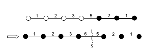
Refer to caption
Figure 22: Acting with S𝑆S-duality on the left part of the graph of figure 21, one obtains a graph with only black dots and a S𝑆S-duality wall.

Starting form an arbitrary linear quiver Tρ^ρ(SU(N))subscriptsuperscript𝑇𝜌^𝜌𝑆𝑈𝑁T^{\rho}_{\hat{\rho}}(SU(N)), one can move all the white dots to the left and all the black dots to the right and then act locally with S𝑆S-duality on the left part of the graph, transforming all the white dots into black dots, as shown in the example of figure 22. The resulting graph has only black dots and a S𝑆S-wall separating the graph into two branches. The left branch of the graph is characterized by the partition ρ^^𝜌\hat{\rho}, the right branch by the partition ρ𝜌\rho and the two branches are glued together through the S𝑆S-wall. The partition function can be read from this graph and has the following structure:

Z(ρ,ρ^)superscript𝑍𝜌^𝜌\displaystyle Z^{(\rho,\hat{\rho})} =dNσ~dNσZbranchρ^[σ~]Sσ~σZbranchρ[σ]absentsuperscript𝑑𝑁~𝜎superscript𝑑𝑁𝜎superscriptsubscript𝑍branch^𝜌delimited-[]~𝜎subscript𝑆~𝜎𝜎superscriptsubscript𝑍branch𝜌delimited-[]𝜎\displaystyle=\int d^{N}\widetilde{\sigma}d^{N}\sigma\ Z_{\rm branch}^{\hat{\rho}}[\widetilde{\sigma}]\ S_{\widetilde{\sigma}\sigma}\ Z_{\rm branch}^{\rho}[\sigma] (5.7)

where Zbranchρ[σ]superscriptsubscript𝑍branch𝜌delimited-[]𝜎Z_{\rm branch}^{\rho}[\sigma] is the partition function of a single black dots-branch, associated to the partition ρ𝜌\rho and the set of eigenvalues {σj}subscript𝜎𝑗\{\sigma_{j}\}. As in 4.2, the partition function of the original theory Zquiversubscript𝑍quiverZ_{\rm quiver} and the partition function associated with the graph with two branches Z(ρ,ρ^)superscript𝑍𝜌^𝜌Z^{(\rho,\hat{\rho})} are equal up to an unphysical phase:

Zquiversubscript𝑍quiver\displaystyle Z_{\rm quiver} =eiφZ(ρ,ρ^),absentsuperscript𝑒𝑖𝜑superscript𝑍𝜌^𝜌\displaystyle=e^{i\,\varphi}\ Z^{(\rho,\hat{\rho})}\ , (5.8)

with φ=2πabmatb𝜑2𝜋subscriptprecedes𝑎𝑏subscript𝑚𝑎subscript𝑡𝑏\varphi=-2\pi\sum_{a\prec b}m_{a}t_{b} and abprecedes𝑎𝑏a\prec b indicates that the D5-brane with parameter masubscript𝑚𝑎m_{a} is placed to the left of the NS5-brane with parameter tbsubscript𝑡𝑏t_{b} in the initial brane sequence realizing the theory.

The single branch partition function for a partition ρ=[(la,ma), 1aP]𝜌delimited-[]subscript𝑙𝑎subscript𝑚𝑎1𝑎𝑃\rho=[\,(l_{a},m_{a})\ ,\ 1\leq a\leq P\ ] of N𝑁N evaluates to:

Zbranchρ[σ]superscriptsubscript𝑍branch𝜌delimited-[]𝜎\displaystyle Z_{\rm branch}^{\rho}[\sigma] =1N!w𝒮N(1)wa=1P(1j=1La1ch(σw(j)maila2)j=1laδ^(σw(j+La1)ma,j))absent1𝑁subscript𝑤superscript𝒮𝑁superscript1𝑤superscriptsubscriptproduct𝑎1𝑃1superscriptsubscriptproduct𝑗1subscript𝐿𝑎1chsubscript𝜎𝑤𝑗subscript𝑚𝑎𝑖subscript𝑙𝑎2superscriptsubscriptproduct𝑗1subscript𝑙𝑎^𝛿subscript𝜎𝑤𝑗subscript𝐿𝑎1subscript𝑚𝑎𝑗\displaystyle=\frac{1}{\sqrt{N!}}\sum_{w\in\mathcal{S}^{N}}(-1)^{w}\prod_{a=1}^{P}\left(\frac{1}{\prod_{j=1}^{L_{a-1}}\textrm{ch}(\sigma_{w(j)}-m_{a}-i\,\frac{l_{a}}{2})}\ \prod_{j=1}^{l_{a}}\hat{\delta}\left(\sigma_{w(j+L_{a-1})}-m_{a,j}\right)\ \right) (5.9)

with Lac=1alcsubscript𝐿𝑎superscriptsubscript𝑐1𝑎subscript𝑙𝑐L_{a}\equiv\sum_{c=1}^{a}l_{c} (LP=Nsubscript𝐿𝑃𝑁L_{P}=N , L0=0subscript𝐿00L_{0}=0) and ma,j=ma+ila+12j2subscript𝑚𝑎𝑗subscript𝑚𝑎𝑖subscript𝑙𝑎12𝑗2m_{a,j}=m_{a}+i\,\frac{l_{a}+1-2j}{2}.

This result can be proved by induction. For P=1𝑃1P=1 the branch has a single black-dot and (5.9) reproduced the associated D5-factor. Then suppose (5.9) is true for a value P𝑃P and take a partition of ρ=[(ma,la), 1aP+1]superscript𝜌delimited-[]subscript𝑚𝑎subscript𝑙𝑎1𝑎𝑃1\rho^{\prime}=[\,(m_{a},l_{a})\ ,\ 1\leq a\leq P+1\ ]. ρsuperscript𝜌\rho^{\prime} is a partition of LP+1=LP+lP+1subscript𝐿𝑃1subscript𝐿𝑃subscript𝑙𝑃1L_{P+1}=L_{P}+l_{P+1}, corresponding to adding one black dot to the graph with P𝑃P dots. Using (5.9), the corresponding matrix model is:

Zbranchρ[σ]=superscriptsubscript𝑍branchsuperscript𝜌delimited-[]superscript𝜎absent\displaystyle Z_{\rm branch}^{\rho^{\prime}}[\sigma^{\prime}]= w𝒮LP+1(1)wdLPσa=1P(1j=1La1ch(σjmaila2)j=1laδ^(σj+La1ma,j))subscriptsuperscript𝑤superscript𝒮subscript𝐿𝑃1superscript1superscript𝑤superscript𝑑subscript𝐿𝑃𝜎superscriptsubscriptproduct𝑎1𝑃1superscriptsubscriptproduct𝑗1subscript𝐿𝑎1chsubscript𝜎𝑗subscript𝑚𝑎𝑖subscript𝑙𝑎2superscriptsubscriptproduct𝑗1subscript𝑙𝑎^𝛿subscript𝜎𝑗subscript𝐿𝑎1subscript𝑚𝑎𝑗\displaystyle\sum_{w^{\prime}\in\mathcal{S}^{L_{P+1}}}(-1)^{w^{\prime}}\int d^{L_{P}}\sigma\ \prod_{a=1}^{P}\left(\frac{1}{\prod_{j=1}^{L_{a-1}}\textrm{ch}(\sigma_{j}-m_{a}-i\,\frac{l_{a}}{2})}\ \prod_{j=1}^{l_{a}}\hat{\delta}\left(\sigma_{j+L_{a-1}}-m_{a,j}\right)\right)
.1LP+1!j=1LPδ(σw(j)σj)j=1LPch(σjmP+1ilP+12)j=1lP+1δ^(σw(j+LP)mP+1,j)\displaystyle\quad.\ \frac{1}{\sqrt{L_{P+1}!}}\ \frac{\prod_{j=1}^{L_{P}}\delta\left(\sigma^{\prime}_{w^{\prime}(j)}-\sigma_{j}\right)}{\prod_{j=1}^{L_{P}}\textrm{ch}(\sigma_{j}-m_{P+1}-i\,\frac{l_{P+1}}{2})}\ \prod_{j=1}^{l_{P+1}}\hat{\delta}\left(\sigma^{\prime}_{w^{\prime}(j+L_{P})}-m_{P+1,j}\right)

where we have de-antisymmetrized the matrix factor (5.9) by permuting the eigenvalues σjsubscript𝜎𝑗\sigma_{j} in the integrand, cancelling an overall 1/LP!1subscript𝐿𝑃1/L_{P}! factor. Integrating over the σjsubscript𝜎𝑗\sigma_{j} using the δ(.)\delta(.) we recover the result (5.9) at level P+1𝑃1P+1, which completes the proof.

We can turn now to the partition function (5.7) of a linear quiver with partitions ρ=[(ma,la), 1aP]𝜌delimited-[]subscript𝑚𝑎subscript𝑙𝑎1𝑎𝑃\rho=[\,(m_{a},l_{a})\ ,\ 1\leq a\leq P\ ], ρ^=[(tb,l^b), 1bP^]^𝜌delimited-[]subscript𝑡𝑏subscript^𝑙𝑏1𝑏^𝑃\hat{\rho}=[\,(t_{b},\hat{l}_{b})\ ,\ 1\leq b\leq\hat{P}\ ] of N𝑁N. De-antisymmetrizing the two branch factors by permuting the σjsubscript𝜎𝑗\sigma_{j} and σ~jsubscript~𝜎𝑗\widetilde{\sigma}_{j} in the integrand leads to:

Z(ρ,ρ^)superscript𝑍𝜌^𝜌\displaystyle Z^{(\rho,\hat{\rho})} =w𝒮N(1)wdNσ^dNσb=1P^(1j=1L^b1ch(σ^jtbil^b2)j=1l^bδ^(σ^j+L^b1tb,j))absentsubscript𝑤subscript𝒮𝑁superscript1𝑤superscript𝑑𝑁^𝜎superscript𝑑𝑁𝜎superscriptsubscriptproduct𝑏1^𝑃1superscriptsubscriptproduct𝑗1subscript^𝐿𝑏1chsubscript^𝜎𝑗subscript𝑡𝑏𝑖subscript^𝑙𝑏2superscriptsubscriptproduct𝑗1subscript^𝑙𝑏^𝛿subscript^𝜎𝑗subscript^𝐿𝑏1subscript𝑡𝑏𝑗\displaystyle=\sum_{w\in\mathcal{S}_{N}}(-1)^{w}\int d^{N}\hat{\sigma}d^{N}\sigma\ \prod_{b=1}^{\hat{P}}\left(\frac{1}{\prod_{j=1}^{\hat{L}_{b-1}}\textrm{ch}(\hat{\sigma}_{j}-t_{b}-i\,\frac{\hat{l}_{b}}{2})}\ \prod_{j=1}^{\hat{l}_{b}}\hat{\delta}\left(\hat{\sigma}_{j+\hat{L}_{b-1}}-t_{b,j}\right)\right)
.e2πijNσ^jσw(j)a=1P(1j=1La1ch(σjmaila2)j=1laδ^(σj+La1ma,j))\displaystyle\quad.\ e^{2\pi i\sum_{j}^{N}\hat{\sigma}_{j}\sigma_{w(j)}}\ \prod_{a=1}^{P}\left(\frac{1}{\prod_{j=1}^{L_{a-1}}\textrm{ch}(\sigma_{j}-m_{a}-i\,\frac{l_{a}}{2})}\ \prod_{j=1}^{l_{a}}\hat{\delta}\left(\sigma_{j+L_{a-1}}-m_{a,j}\right)\right)

The integration must now be carried out using the δ^(.)\hat{\delta}(.). The result of such integration contains generally a regular piece obtained by treating the δ^^𝛿\hat{\delta} as simple δ𝛿\delta functions plus a complicated sum of terms involving products of δ^(.)\hat{\delta}(.). However in our case we know that the matrix model evaluates to a regular finite result as it is equal to the matrix model of a good linear quiver. This means that the singular terms with δ^(.)\hat{\delta}(.) all cancel in the anti-symetrization by w𝒮Nsubscript𝑤subscript𝒮𝑁\sum_{w\in\mathcal{S}_{N}}, so we can evaluate the result by treating the δ^(.)\hat{\delta}(.) as usual δ(.)\delta(.) functions.191919We have verified this property explicitly in simple examples. This leads directly to the NTY conjectured formula:202020Our formula correct some overall factor mistake in the NTY formula.

Z(ρ,ρ^)=w𝒮N(1)we2πijNTjMw(j)Δ(T)Δ(M)superscript𝑍𝜌^𝜌subscript𝑤superscript𝒮𝑁superscript1𝑤superscript𝑒2𝜋𝑖superscriptsubscript𝑗𝑁subscript𝑇𝑗subscript𝑀𝑤𝑗Δ𝑇Δ𝑀\displaystyle Z^{(\rho,\hat{\rho})}=\frac{\sum_{w\in\mathcal{S}^{N}}(-1)^{w}e^{2\pi i\,\sum_{j}^{N}T_{j}M_{w(j)}}}{\Delta(T)\Delta(M)} (5.10) withΔ(M)=a=1Pj=1La1ch(Mjmaila2),Δ(T)=b=1P^j=1L^b1ch(Tjtbil^b2)formulae-sequencewithΔ𝑀superscriptsubscriptproduct𝑎1𝑃superscriptsubscriptproduct𝑗1subscript𝐿𝑎1chsubscript𝑀𝑗subscript𝑚𝑎𝑖subscript𝑙𝑎2Δ𝑇superscriptsubscriptproduct𝑏1^𝑃superscriptsubscriptproduct𝑗1subscript^𝐿𝑏1chsubscript𝑇𝑗subscript𝑡𝑏𝑖subscript^𝑙𝑏2\displaystyle\textrm{with}\quad\Delta(M)=\prod_{a=1}^{P}\prod_{j=1}^{L_{a-1}}\textrm{ch}\left(M_{j}-m_{a}-i\,\frac{l_{a}}{2}\right)\ ,\quad\Delta(T)=\prod_{b=1}^{\hat{P}}\prod_{j=1}^{\hat{L}_{b-1}}\textrm{ch}\left(T_{j}-t_{b}-i\,\frac{\hat{l}_{b}}{2}\right)

and M𝑀M and T𝑇T are the N𝑁N-vectors defined in (5). As pointed in [26], the result is explicitly symmetric under the exchange of the deformed partitions ρ𝜌\rho and ρ^^𝜌\hat{\rho}.

As a simple consistency check of the validity of our manipulations of matrix models, we provide in appendix C.3 an explicit computation mapping the matrix model of a separated graph (black dots on the right, white dots on the left) to the matrix model of the initial quiver theory.

6 Perspectives

We have shown how the matrix model giving the exact partition function of an 𝒩=4𝒩4\mathcal{N}=4 theory on S3superscript𝑆3S^{3} can be expressed as a sequence of elementary factors, mimicking the sequence of 5-branes of its brane realization in type IIB string theory. We have described the action of SL(2,)𝑆𝐿2SL(2,\mathbb{Z}) dualities on these 5-brane factors and shown that the partition functions of SL(2,)𝑆𝐿2SL(2,\mathbb{Z}) dual theories are equal, up to a phase, which was unphysical in all cases we studied. We found that the Hanany-Witten 5-brane move is expressed by a non-trivial identity for 5-brane blocks that we proved. This allowed us to map the partition functions of Yang-Mills mirror-dual theories for linear and circular quivers with unitary nodes of arbitrary ranks, providing a significant extension of the results of [7]. In addition our results go beyond simple mirror symmetry and provide maps between the partition functions for a large web of dualities, generated by SL(2,)𝑆𝐿2SL(2,\mathbb{Z}) actions and 5-brane moves. These involve 𝒩=4𝒩4\mathcal{N}=4 level-rank dualities and dualities relating Yang-Mills to Chern-Simons quiver theories.

There are several extensions one can think of. It would be nice to consider the cases of quivers with orthogonal and symplectic gauge nodes realized by brane configurations involving orientifold planes [10] and see if a similar story exists. At the technical level one can try to consider the partition functions on a squashed 3-sphere Sb3subscriptsuperscript𝑆3𝑏S^{3}_{b} instead of the round S3superscript𝑆3S^{3}, providing stronger tests of the dualities. An interesting question, which we did not address at all, is the question of how the moduli spaces of the SL(2,)𝑆𝐿2SL(2,\mathbb{Z}) dual theories are mapped and how they are affected or not by quantum corrections. Usual mirror symmetry is known to exchange the Coulomb and Higgs branches of dual Yang-Mills theories, the Higgs branch being classically exact (no quantum correction). It would be natural to investigate the properties of the moduli space of dual Chern-Simons theories, as was done in [17].

Acknowledgments

We thank Jaume Gomis for sharing ideas, in particular on the possible Chern-Simons description of Yang-Mills fixed points, and for many interesting discussions. We thank Nadav Drukker for comments on the manuscript. We thank the Perimeter Institute for hospitality during a visit. This work was supported by the ERC Starting Grant N. 304806, “The Gauge/Gravity Duality and Geometry in String Theory”. Research at the Perimeter Institute is supported in part by the Government of Canada through NSERC and by the Province of Ontario through MRI.

Appendix A δ^^𝛿\hat{\delta} distributions

In this paper we consider integrations of meromorphic functions with simple poles, whose integral on the real line is convergent. When a pole lies on the integration contour we choose the principal value prescription to integrate.

Formally, the function xδ^(xz0)𝑥^𝛿𝑥subscript𝑧0x\rightarrow\hat{\delta}(x-z_{0}), with x,z0formulae-sequence𝑥subscript𝑧0x\in\mathbb{R},z_{0}\in\mathbb{C}, is meant to be the Fourier transform of the function xe2πiz0x𝑥superscript𝑒2𝜋𝑖subscript𝑧0𝑥x\rightarrow e^{-2\pi iz_{0}x}, generalizing the usual Dirac distribution to complex z0subscript𝑧0z_{0}:

δ^(xz0)=dye2πiy(xz0),x,z0.\displaystyle\hat{\delta}(x-z_{0})=\int_{\mathbb{R}}dy\ e^{2\pi iy(x-z_{0})}\quad,\quad x\in\mathbb{R}\,,\,z_{0}\in\mathbb{C}\ . (A.1)

With f𝑓f a meromorphic function on \mathbb{C} with simple poles away from z0subscript𝑧0z_{0}. Concretely we define the δ^z0δ^(.z0)\hat{\delta}_{z_{0}}\equiv\hat{\delta}(\,.-z_{0}) distribution by the recursion relation:

𝑑xδ^(xz0)f(x)subscriptdifferential-d𝑥^𝛿𝑥subscript𝑧0𝑓𝑥\displaystyle\int_{\mathbb{R}}dx\ \hat{\delta}(x-z_{0})f(x) =f(z0)+ 2πiϵ(z0)jδ^(ujz0)f^(uj)absent𝑓subscript𝑧02𝜋𝑖italic-ϵsubscript𝑧0subscript𝑗^𝛿subscript𝑢𝑗subscript𝑧0^𝑓subscript𝑢𝑗\displaystyle=f(z_{0})\ +\ 2\pi i\epsilon(z_{0})\sum_{j}\hat{\delta}(u_{j}-z_{0})\hat{f}(u_{j}) (A.2)

where ϵ(z0)=italic-ϵsubscript𝑧0absent\epsilon(z_{0})=\ sgn(Im(z0)subscript𝑧0(z_{0})) and ujsubscript𝑢𝑗u_{j} are the poles of f𝑓f in the region 00absent0\leqIm(u)𝑢absent(u)\leqIm(z0)subscript𝑧0(z_{0}) for ϵ(z0)=+1italic-ϵsubscript𝑧01\epsilon(z_{0})=+1 or the region Im(z0)subscript𝑧0absent(z_{0})\leqIm(u)0𝑢0(u)\leq 0 for ϵ(z0)=1italic-ϵsubscript𝑧01\epsilon(z_{0})=-1. When 0<|0<|Im(uj)|<|(u_{j})|<|Im(z0)|(z_{0})|, f^(uj)^𝑓subscript𝑢𝑗\hat{f}(u_{j}) is the residue at the pole ujsubscript𝑢𝑗u_{j}. When Im(uj)=0subscript𝑢𝑗0(u_{j})=0 or Im(uj)=subscript𝑢𝑗absent(u_{j})=Im(z0)subscript𝑧0(z_{0}), f^(uj)^𝑓subscript𝑢𝑗\hat{f}(u_{j}) is half the residue at the pole ujsubscript𝑢𝑗u_{j}. This definition comes down to shifting the contour of the x𝑥x integration from \mathbb{R} to +i𝑖\mathbb{R}+iIm(z0)subscript𝑧0(z_{0}), picking pole residues, as can be understood from the heuristic derivation:

𝑑xδ^(xz0)subscriptdifferential-d𝑥^𝛿𝑥subscript𝑧0\displaystyle\int_{\mathbb{R}}dx\ \hat{\delta}(x-z_{0}) f(x)=𝑑x𝑑σe2πi(xz0)σf(x)=𝑑σ𝑑xe2πi(xz0)σf(x)𝑓𝑥subscriptdifferential-d𝑥subscriptdifferential-d𝜎superscript𝑒2𝜋𝑖𝑥subscript𝑧0𝜎𝑓𝑥subscriptdifferential-d𝜎subscriptdifferential-d𝑥superscript𝑒2𝜋𝑖𝑥subscript𝑧0𝜎𝑓𝑥\displaystyle f(x)\ =\ \int_{\mathbb{R}}dx\int_{\mathbb{R}}d\sigma\ e^{2\pi i(x-z_{0})\sigma}f(x)\ =\int_{\mathbb{R}}d\sigma\int_{\mathbb{R}}dx\ e^{2\pi i(x-z_{0})\sigma}f(x)
=𝑑σ(𝑑xe2πi(xRe(z0))σf(x+iIm(z0))+2πiϵ(z0)je2πi(ujz0)σf^(uj))absentsubscriptdifferential-d𝜎subscriptdifferential-d𝑥superscript𝑒2𝜋𝑖𝑥𝑅𝑒subscript𝑧0𝜎𝑓𝑥𝑖Imsubscript𝑧02𝜋𝑖italic-ϵsubscript𝑧0subscript𝑗superscript𝑒2𝜋𝑖subscript𝑢𝑗subscript𝑧0𝜎^𝑓subscript𝑢𝑗\displaystyle=\int_{\mathbb{R}}d\sigma\left(\int_{\mathbb{R}}dx\ e^{2\pi i(x-Re(z_{0}))\sigma}f(x+i{\rm Im}(z_{0}))+2\pi i\epsilon(z_{0})\sum_{j}e^{2\pi i(u_{j}-z_{0})\sigma}\hat{f}(u_{j})\right)
=f(z0)+2πiϵ(z0)jδ^(ujz0)f^(uj)absent𝑓subscript𝑧02𝜋𝑖italic-ϵsubscript𝑧0subscript𝑗^𝛿subscript𝑢𝑗subscript𝑧0^𝑓subscript𝑢𝑗\displaystyle=f(z_{0})+2\pi i\epsilon(z_{0})\sum_{j}\hat{\delta}(u_{j}-z_{0})\hat{f}(u_{j})

where at the second line we have moved the contour of integration of x𝑥x to +i𝑖\mathbb{R}+iIm(z0)subscript𝑧0(z_{0}), picking pole residues, and made a change of variable xx+i𝑥𝑥𝑖x\rightarrow x+iIm(z0)subscript𝑧0(z_{0}).

The definition (A.2) implies

δ^(xz0)g(x)=δ^(xz0)g(z0),^𝛿𝑥subscript𝑧0𝑔𝑥^𝛿𝑥subscript𝑧0𝑔subscript𝑧0\displaystyle\hat{\delta}(x-z_{0})g(x)=\hat{\delta}(x-z_{0})g(z_{0})\ , (A.3)

for any function g𝑔g without poles on the complex plane (or simply without poles in the region 00absent0\leqIm(u)𝑢absent(u)\leqIm(z0)subscript𝑧0(z_{0})). 212121This formula can be applied in an integral as 𝑑xf(x)g(x)δ^(xz0)=𝑑xf(x)g(z0)δ^(xz0)differential-d𝑥𝑓𝑥𝑔𝑥^𝛿𝑥subscript𝑧0differential-d𝑥𝑓𝑥𝑔subscript𝑧0^𝛿𝑥subscript𝑧0\int dx\,f(x)g(x)\hat{\delta}(x-z_{0})=\int dx\,f(x)g(z_{0})\hat{\delta}(x-z_{0}), as long as f𝑓f does not have a pole at z0subscript𝑧0z_{0}. It may happen that g(z0)=0𝑔subscript𝑧00g(z_{0})=0 and f𝑓f has a pole at z0subscript𝑧0z_{0}, so that the integral yields a finite result, in which case (A.3) is not valid.

When dealing with multiple integrals, the δ^^𝛿\hat{\delta} distribution can lead to shifts of contours of integration. For instance:

𝑑x𝑑x~δ^(x~xiy0)f(x)g(x~)=𝒞(y0)𝑑xf(x)gy0(x),subscriptdifferential-d𝑥subscriptdifferential-d~𝑥^𝛿~𝑥𝑥𝑖subscript𝑦0𝑓𝑥𝑔~𝑥subscript𝒞subscript𝑦0differential-d𝑥𝑓𝑥subscript𝑔subscript𝑦0𝑥\displaystyle\int_{\mathbb{R}}dx\int_{\mathbb{R}}d\widetilde{x}\ \hat{\delta}(\widetilde{x}-x-iy_{0})f(x)g(\widetilde{x})=\int_{\mathcal{C}(y_{0})}dx\ f(x)g_{y_{0}}(x)\ , (A.4)

where y0subscript𝑦0y_{0}\in\mathbb{R}, gy0(x)=g(x+iy0)subscript𝑔subscript𝑦0𝑥𝑔𝑥𝑖subscript𝑦0g_{y_{0}}(x)=g(x+iy_{0}), and the final contour of integration 𝒞(y0)𝒞subscript𝑦0\mathcal{C}(y_{0}) of x𝑥x is obtained by deforming the real line \mathbb{R} to a curve in \mathbb{C} in such a way that, for y00subscript𝑦00y_{0}\geq 0, the contour passes below the poles u𝑢u of gy0subscript𝑔subscript𝑦0g_{y_{0}} in the region y0subscript𝑦0absent-y_{0}\leqIm(u)0𝑢0(u)\leq 0, or for y00subscript𝑦00y_{0}\leq 0, the contour passes above the poles u𝑢u of gy0subscript𝑔subscript𝑦0g_{y_{0}} in the region 00absent0\leqIm(ug)y0subscript𝑢𝑔subscript𝑦0(u_{g})\leq-y_{0}, while the poles of f𝑓f stay on the same side of the contour.

Appendix B Formulas

This appendix contains some formulas we used in our compuations.

  • Weyl denominator formula

    i<jNsh(σiσj)=w𝒮N(1)we2πj=1NσjWw(j)(N)superscriptsubscriptproduct𝑖𝑗𝑁shsubscript𝜎𝑖subscript𝜎𝑗subscript𝑤superscript𝒮𝑁superscript1𝑤superscript𝑒2𝜋superscriptsubscript𝑗1𝑁subscript𝜎𝑗subscriptsuperscript𝑊𝑁𝑤𝑗\displaystyle\prod_{i<j}^{N}\textrm{sh}(\sigma_{i}-\sigma_{j})=\sum_{w\in\mathcal{S}^{N}}(-1)^{w}\ e^{2\pi\sum_{j=1}^{N}\sigma_{j}W^{(N)}_{w(j)}} (B.1)

    where W(N)superscript𝑊𝑁W^{(N)} is the Weyl vector of U(N)𝑈𝑁U(N): Wj(N)=N+12j2subscriptsuperscript𝑊𝑁𝑗𝑁12𝑗2W^{(N)}_{j}=\frac{N+1-2j}{2}, j=1,,N𝑗1𝑁j=1,\cdots,N.

  • Cauchy determinant formula

    i<jNsh(σiσj)i<jNsh(σ~iσ~j)i,jNch(σiσ~j)=w𝒮N(1)w1jNch(σw(j)σ~j).superscriptsubscriptproduct𝑖𝑗𝑁shsubscript𝜎𝑖subscript𝜎𝑗superscriptsubscriptproduct𝑖𝑗𝑁shsubscript~𝜎𝑖subscript~𝜎𝑗superscriptsubscriptproduct𝑖𝑗𝑁chsubscript𝜎𝑖subscript~𝜎𝑗subscript𝑤superscript𝒮𝑁superscript1𝑤1superscriptsubscriptproduct𝑗𝑁chsubscript𝜎𝑤𝑗subscript~𝜎𝑗\displaystyle\frac{\prod_{i<j}^{N}\textrm{sh}(\sigma_{i}-\sigma_{j})\prod_{i<j}^{N}\textrm{sh}(\widetilde{\sigma}_{i}-\widetilde{\sigma}_{j})}{\prod_{i,j}^{N}\textrm{ch}(\sigma_{i}-\widetilde{\sigma}_{j})}=\sum_{w\in\mathcal{S}^{N}}(-1)^{w}\frac{1}{\prod_{j}^{N}\textrm{ch}(\sigma_{w(j)}-\widetilde{\sigma}_{j})}\ . (B.2)

    A generalized version of this formula is, for NN~𝑁~𝑁N\geq\widetilde{N}, ΔNN~Δ𝑁~𝑁\Delta\equiv N-\widetilde{N}:

    i<jNsh(σiσj)i<jN~sh(σ~iσ~j)iNjN~ch(σiσ~j)superscriptsubscriptproduct𝑖𝑗𝑁shsubscript𝜎𝑖subscript𝜎𝑗superscriptsubscriptproduct𝑖𝑗~𝑁shsubscript~𝜎𝑖subscript~𝜎𝑗superscriptsubscriptproduct𝑖𝑁superscriptsubscriptproduct𝑗~𝑁chsubscript𝜎𝑖subscript~𝜎𝑗\displaystyle\frac{\prod_{i<j}^{N}\textrm{sh}(\sigma_{i}-\sigma_{j})\prod_{i<j}^{\widetilde{N}}\textrm{sh}(\widetilde{\sigma}_{i}-\widetilde{\sigma}_{j})}{\prod_{i}^{N}\prod_{j}^{\widetilde{N}}\textrm{ch}(\sigma_{i}-\widetilde{\sigma}_{j})}
    =(1)ΔN~w𝒮N(1)wj=1N~eπΔ(σw(j)σ~j)ch(σw(j)σ~j)j=N~+1Ne2πσw(j)(N+N~+12j)absentsuperscript1Δ~𝑁subscript𝑤superscript𝒮𝑁superscript1𝑤superscriptsubscriptproduct𝑗1~𝑁superscript𝑒𝜋Δsubscript𝜎𝑤𝑗subscript~𝜎𝑗chsubscript𝜎𝑤𝑗subscript~𝜎𝑗superscriptsubscriptproduct𝑗~𝑁1𝑁superscript𝑒2𝜋subscript𝜎𝑤𝑗𝑁~𝑁12𝑗\displaystyle\qquad=(-1)^{\Delta\widetilde{N}}\sum_{w\in\mathcal{S}^{N}}(-1)^{w}\prod_{j=1}^{\widetilde{N}}\frac{e^{-\pi\Delta(\sigma_{w(j)}-\widetilde{\sigma}_{j})}}{\textrm{ch}(\sigma_{w(j)}-\widetilde{\sigma}_{j})}\ \prod_{j=\widetilde{N}+1}^{N}e^{2\pi\sigma_{w(j)}\left(\frac{N+\widetilde{N}+1}{2}-j\right)} (B.3)

    This formula was derived from a similar formula in [41] 222222we use their formula with xj=e2πσ~jsubscript𝑥𝑗superscript𝑒2𝜋subscript~𝜎𝑗x_{j}=e^{2\pi\widetilde{\sigma}_{j}}, yj=e2πσjsubscript𝑦𝑗superscript𝑒2𝜋subscript𝜎𝑗y_{j}=e^{2\pi\sigma_{j}}.

  • Others identities, for p𝑝p\in\mathbb{N}, x𝑥x\in\mathbb{C} :

    j=1p2sinh[πp(x+ip+12ij)]={2cosh(πx),peven2sinh(πx),podd\displaystyle\prod_{j=1}^{p}2\sinh\Big{[}\frac{\pi}{p}\left(x+i\,\frac{p+1}{2}-ij\right)\Big{]}=\left\{\begin{array}[]{c}2\cosh(\pi x)\quad,\quad p\ {\rm even}\\ 2\sinh(\pi x)\quad,\quad p\ {\rm odd}\end{array}\right. (B.6)
    j=1p2cosh[πp(x+ip+12ij)]=2cosh(πx)superscriptsubscriptproduct𝑗1𝑝2𝜋𝑝𝑥𝑖𝑝12𝑖𝑗2𝜋𝑥\displaystyle\prod_{j=1}^{p}2\cosh\Big{[}\frac{\pi}{p}\left(x+i\,\frac{p+1}{2}-ij\right)\Big{]}=2\cosh(\pi x) (B.7)
    1j<kp2sinh(iπp(kj))=ip(p1)2pp2,subscriptproduct1𝑗𝑘𝑝2𝑖𝜋𝑝𝑘𝑗superscript𝑖𝑝𝑝12superscript𝑝𝑝2\displaystyle\prod_{1\leq j<k\leq p}2\sinh\left(\frac{i\pi}{p}(k-j)\right)=i^{\frac{p(p-1)}{2}}\,p^{\frac{p}{2}}\ ,

    and more generally for A,B𝐴𝐵A,B\in\mathbb{N} with p=A+B𝑝𝐴𝐵p=A+B :

    j=1A2sinh[πp(x+iA+12ij)]j=1B2cosh[πp(x+iB+12ij)]superscriptsubscriptproduct𝑗1𝐴2𝜋𝑝𝑥𝑖𝐴12𝑖𝑗superscriptsubscriptproduct𝑗1𝐵2𝜋𝑝𝑥𝑖𝐵12𝑖𝑗\displaystyle\prod_{j=1}^{A}2\sinh\Big{[}\frac{\pi}{p}\left(x+i\,\frac{A+1}{2}-ij\right)\Big{]}\prod_{j=1}^{B}2\cosh\Big{[}\frac{\pi}{p}\left(x+i\,\frac{B+1}{2}-ij\right)\Big{]}
    ={2cosh(πx),Aeven2sinh(πx),Aodd\displaystyle\qquad=\left\{\begin{array}[]{c}2\cosh(\pi x)\quad,\quad A\ {\rm even}\\ 2\sinh(\pi x)\quad,\quad A\ {\rm odd}\end{array}\right. (B.10)
    (i)A(A1)2pA21j<kA2sinh(iπp(kj))=(i)B(B1)2pB21j<kB2sinh(iπp(kj)).superscript𝑖𝐴𝐴12superscript𝑝𝐴2subscriptproduct1𝑗𝑘𝐴2𝑖𝜋𝑝𝑘𝑗superscript𝑖𝐵𝐵12superscript𝑝𝐵2subscriptproduct1𝑗𝑘𝐵2𝑖𝜋𝑝𝑘𝑗\displaystyle(-i)^{\frac{A(A-1)}{2}}p^{-\frac{A}{2}}\prod_{1\leq j<k\leq A}2\sinh\left(\frac{i\pi}{p}(k-j)\right)=(-i)^{\frac{B(B-1)}{2}}p^{-\frac{B}{2}}\prod_{1\leq j<k\leq B}2\sinh\left(\frac{i\pi}{p}(k-j)\right)\ . (B.11)

    We tested these formulas with Mathematica for small values of p𝑝p, but did not prove them in general.

Appendix C Computations

In this appendix we present computations.

C.1 Local S𝑆S-transformations

We assume Δ=NN~0Δ𝑁~𝑁0\Delta=N-\widetilde{N}\geq 0, p0𝑝0p\neq 0, q0𝑞0q\neq 0 and we remind μ=N+N~2𝜇𝑁~𝑁2\mu=\frac{N+\widetilde{N}}{2}.

(S[pq]S1)σσ~=dNτdN~τ~e2πijNσjτj[pq]ττ~e2πijN~τ~jσ~jsubscript𝑆delimited-[]𝑝𝑞superscript𝑆1𝜎~𝜎superscript𝑑𝑁𝜏superscript𝑑~𝑁~𝜏superscript𝑒2𝜋𝑖superscriptsubscript𝑗𝑁subscript𝜎𝑗subscript𝜏𝑗subscriptdelimited-[]𝑝𝑞𝜏~𝜏superscript𝑒2𝜋𝑖superscriptsubscript𝑗~𝑁subscript~𝜏𝑗subscript~𝜎𝑗\displaystyle\left(S{\left[\begin{array}[]{c}p\\ q\end{array}\right]}S^{-1}\right)_{\sigma\,\widetilde{\sigma}}=\int d^{N}\tau d^{\widetilde{N}}\widetilde{\tau}\ e^{2\pi i\sum_{j}^{N}\sigma_{j}\tau_{j}}\ {\left[\begin{array}[]{c}p\\ q\end{array}\right]}_{\tau\,\widetilde{\tau}}\ e^{-2\pi i\sum_{j}^{\widetilde{N}}\widetilde{\tau}_{j}\widetilde{\sigma}_{j}}
=|p|μN!N~!dNτdN~τ~e2πijNσjτje2πitp(jNτjjN~τ~j)absentsuperscript𝑝𝜇𝑁~𝑁superscript𝑑𝑁𝜏superscript𝑑~𝑁~𝜏superscript𝑒2𝜋𝑖superscriptsubscript𝑗𝑁subscript𝜎𝑗subscript𝜏𝑗superscript𝑒2𝜋𝑖𝑡𝑝superscriptsubscript𝑗𝑁subscript𝜏𝑗superscriptsubscript𝑗~𝑁subscript~𝜏𝑗\displaystyle=\frac{|p|^{-\mu}}{\sqrt{N!\widetilde{N}!}}\int d^{N}\tau d^{\widetilde{N}}\widetilde{\tau}\ e^{2\pi i\sum_{j}^{N}\sigma_{j}\tau_{j}}\ e^{-2\pi i\frac{t}{p}\left(\sum_{j}^{N}\tau_{j}-\sum_{j}^{\widetilde{N}}\widetilde{\tau}_{j}\right)}
.eπiqp(jNτj2jN~τ~j2)i<jNsh[p1τij]i<jN~sh[p1τ~ij]i,jN,N~ch[p1(τiτ~j)]e2πijN~τ~jσ~j\displaystyle\hskip 113.81102pt.\ e^{\pi i\,\frac{q}{p}\left(\sum_{j}^{N}\tau_{j}^{2}-\sum_{j}^{\widetilde{N}}\widetilde{\tau}_{j}^{2}\right)}\ \frac{\prod_{i<j}^{N}\textrm{sh}[\,p^{-1}\tau_{ij}]\ \prod_{i<j}^{\widetilde{N}}\textrm{sh}[\,p^{-1}\widetilde{\tau}_{ij}]}{\prod_{i,j}^{N,\widetilde{N}}\textrm{ch}[\,p^{-1}(\tau_{i}-\widetilde{\tau}_{j})]}\ e^{-2\pi i\sum_{j}^{\widetilde{N}}\widetilde{\tau}_{j}\widetilde{\sigma}_{j}}
=|p|μN!N~!dNτdN~τ~e2πijNτj(pσjt)eπipq(jNτj2jN~τ~j2)absentsuperscript𝑝𝜇𝑁~𝑁superscript𝑑𝑁𝜏superscript𝑑~𝑁~𝜏superscript𝑒2𝜋𝑖superscriptsubscript𝑗𝑁subscript𝜏𝑗𝑝subscript𝜎𝑗𝑡superscript𝑒𝜋𝑖𝑝𝑞superscriptsubscript𝑗𝑁superscriptsubscript𝜏𝑗2superscriptsubscript𝑗~𝑁superscriptsubscript~𝜏𝑗2\displaystyle=\frac{|p|^{\mu}}{\sqrt{N!\widetilde{N}!}}\int d^{N}\tau d^{\widetilde{N}}\widetilde{\tau}\ e^{2\pi i\sum_{j}^{N}\tau_{j}(p\sigma_{j}-t)}\ e^{\pi i\,pq\left(\sum_{j}^{N}\tau_{j}^{2}-\sum_{j}^{\widetilde{N}}\widetilde{\tau}_{j}^{2}\right)}
.i<jNsh(τij)i<jN~sh(τ~ij)i,jN,N~ch(τiτ~j)e2πijN~τ~j(pσ~jt)\displaystyle\hskip 113.81102pt.\ \frac{\prod_{i<j}^{N}\textrm{sh}(\tau_{ij})\ \prod_{i<j}^{\widetilde{N}}\textrm{sh}(\widetilde{\tau}_{ij})}{\prod_{i,j}^{N,\widetilde{N}}\textrm{ch}(\tau_{i}-\widetilde{\tau}_{j})}\ e^{-2\pi i\sum_{j}^{\widetilde{N}}\widetilde{\tau}_{j}(p\widetilde{\sigma}_{j}-t)}
=|p|μN!N~!(1)ΔN~w𝒮N(1)wdNτdN~τ~e2πijNτj(pσjt)eπipq(jNτj2jN~τ~j2)absentsuperscript𝑝𝜇𝑁~𝑁superscript1Δ~𝑁subscript𝑤superscript𝒮𝑁superscript1𝑤superscript𝑑𝑁𝜏superscript𝑑~𝑁~𝜏superscript𝑒2𝜋𝑖superscriptsubscript𝑗𝑁subscript𝜏𝑗𝑝subscript𝜎𝑗𝑡superscript𝑒𝜋𝑖𝑝𝑞superscriptsubscript𝑗𝑁superscriptsubscript𝜏𝑗2superscriptsubscript𝑗~𝑁superscriptsubscript~𝜏𝑗2\displaystyle=\frac{|p|^{\mu}}{\sqrt{N!\widetilde{N}!}}(-1)^{\Delta\widetilde{N}}\sum_{w\in\mathcal{S}^{N}}(-1)^{w}\int d^{N}\tau d^{\widetilde{N}}\widetilde{\tau}\ e^{2\pi i\sum_{j}^{N}\tau_{j}(p\sigma_{j}-t)}\ e^{\pi i\,pq\left(\sum_{j}^{N}\tau_{j}^{2}-\sum_{j}^{\widetilde{N}}\widetilde{\tau}_{j}^{2}\right)}
.j=1N~eΔ(τw(j)τ~j)ch(τw(j)τ~j)j=N~+1Ne2πτw(j)(μ+12j)e2πijN~τ~j(pσ~jt)\displaystyle\hskip 113.81102pt\ .\ \prod_{j=1}^{\widetilde{N}}\frac{e^{-\Delta(\tau_{w(j)}-\widetilde{\tau}_{j})}}{\textrm{ch}(\tau_{w(j)}-\widetilde{\tau}_{j})}\prod_{j=\widetilde{N}+1}^{N}e^{2\pi\tau_{w(j)}\left(\mu+\frac{1}{2}-j\right)}\ e^{-2\pi i\sum_{j}^{\widetilde{N}}\widetilde{\tau}_{j}(p\widetilde{\sigma}_{j}-t)}

where we have rescaled τj,τ~jpτj,pτ~jformulae-sequencesubscript𝜏𝑗subscript~𝜏𝑗𝑝subscript𝜏𝑗𝑝subscript~𝜏𝑗\tau_{j},\widetilde{\tau}_{j}\rightarrow p\tau_{j},p\widetilde{\tau}_{j} (3rd equality) and used the generalized Cauchy determinant formula (B.3).

In each integral we can reshuffle the eigenvalues τw(j)τjsubscript𝜏𝑤𝑗subscript𝜏𝑗\tau_{w(j)}\rightarrow\tau_{j} for j=1,,N𝑗1𝑁j=1,\cdots,N and then shift τw(j)τw(j)+τ~jsubscript𝜏𝑤𝑗subscript𝜏𝑤𝑗subscript~𝜏𝑗\tau_{w(j)}\rightarrow\tau_{w(j)}+\widetilde{\tau}_{j} for j=1,,N~𝑗1~𝑁j=1,\cdots,\widetilde{N} to obtain

=(1)ΔN~|p|μN!N~!w𝒮N(1)wdNτdN~τ~e2πijNτj(pσw(j)t)eπipqjNτj2absentsuperscript1Δ~𝑁superscript𝑝𝜇𝑁~𝑁subscript𝑤superscript𝒮𝑁superscript1𝑤superscript𝑑𝑁𝜏superscript𝑑~𝑁~𝜏superscript𝑒2𝜋𝑖superscriptsubscript𝑗𝑁subscript𝜏𝑗𝑝subscript𝜎𝑤𝑗𝑡superscript𝑒𝜋𝑖𝑝𝑞superscriptsubscript𝑗𝑁superscriptsubscript𝜏𝑗2\displaystyle=(-1)^{\Delta\widetilde{N}}\frac{|p|^{\mu}}{\sqrt{N!\widetilde{N}!}}\sum_{w\in\mathcal{S}^{N}}(-1)^{w}\int d^{N}\tau d^{\widetilde{N}}\widetilde{\tau}\ e^{2\pi i\sum_{j}^{N}\tau_{j}(p\sigma_{w(j)}-t)}\ e^{\pi i\,pq\sum_{j}^{N}\tau_{j}^{2}}
.j=1N~eΔτjch(τj)j=N~+1Ne2πτj(μ+12j)e2πipjN~τ~j(σw(j)+qτjσ~j)\displaystyle\hskip 113.81102pt\ .\ \prod_{j=1}^{\widetilde{N}}\frac{e^{-\Delta\tau_{j}}}{\textrm{ch}(\tau_{j})}\prod_{j=\widetilde{N}+1}^{N}e^{2\pi\tau_{j}\left(\mu+\frac{1}{2}-j\right)}\ e^{2\pi i\,p\sum_{j}^{\widetilde{N}}\widetilde{\tau}_{j}(\sigma_{w(j)}+q\tau_{j}-\widetilde{\sigma}_{j})}

Integrating over the τ~jsubscript~𝜏𝑗\widetilde{\tau}_{j} yields δ[p(σw(j)+qτjσ~j)]𝛿delimited-[]𝑝subscript𝜎𝑤𝑗𝑞subscript𝜏𝑗subscript~𝜎𝑗\delta[p(\sigma_{w(j)}+q\tau_{j}-\widetilde{\sigma}_{j})] that can be used to integrate over the τjsubscript𝜏𝑗\tau_{j} for j=1,,N~𝑗1~𝑁j=1,\cdots,\widetilde{N} (since pq0𝑝𝑞0pq\neq 0). We get

=(1)ΔN~|q|N~|p|Δ2N!N~!w𝒮N(1)wdΔτe2πij=N~+1Nτj(pσw(j)t)e2πiqjN~(σ~jσw(j))(pσw(j)t)absentsuperscript1Δ~𝑁superscript𝑞~𝑁superscript𝑝Δ2𝑁~𝑁subscript𝑤superscript𝒮𝑁superscript1𝑤superscript𝑑Δ𝜏superscript𝑒2𝜋𝑖superscriptsubscript𝑗~𝑁1𝑁subscript𝜏𝑗𝑝subscript𝜎𝑤𝑗𝑡superscript𝑒2𝜋𝑖𝑞superscriptsubscript𝑗~𝑁subscript~𝜎𝑗subscript𝜎𝑤𝑗𝑝subscript𝜎𝑤𝑗𝑡\displaystyle=(-1)^{\Delta\widetilde{N}}\frac{|q|^{-\widetilde{N}}|p|^{\frac{\Delta}{2}}}{\sqrt{N!\widetilde{N}!}}\sum_{w\in\mathcal{S}^{N}}(-1)^{w}\int d^{\Delta}\tau\ e^{2\pi i\sum_{j=\widetilde{N}+1}^{N}\tau_{j}(p\sigma_{w(j)}-t)}\ e^{\frac{2\pi i}{q}\sum_{j}^{\widetilde{N}}(\widetilde{\sigma}_{j}-\sigma_{w(j)})(p\sigma_{w(j)}-t)}
.eπipqjN~(σ~jσw(j))2eπipqj=N~+1Nτj2j=1N~eΔq(σ~jσw(j))ch[q1(σ~jσw(j))]j=N~+1Ne2πτj(μ+12j)\displaystyle\hskip 85.35826pt\ .\ e^{\pi i\,\frac{p}{q}\sum_{j}^{\widetilde{N}}(\widetilde{\sigma}_{j}-\sigma_{w(j)})^{2}}e^{\pi i\,pq\sum_{j=\widetilde{N}+1}^{N}\tau_{j}^{2}}\ \prod_{j=1}^{\widetilde{N}}\frac{e^{-\frac{\Delta}{q}(\widetilde{\sigma}_{j}-\sigma_{w(j)})}}{\textrm{ch}[q^{-1}(\widetilde{\sigma}_{j}-\sigma_{w(j)})]}\prod_{j=\widetilde{N}+1}^{N}e^{2\pi\tau_{j}\left(\mu+\frac{1}{2}-j\right)}
=(1)ΔN~|q|N~|p|Δ2N!N~!w𝒮N(1)weπipqjN~(σ~jσw(j))2e2πipqjN~(σ~jσw(j))(σw(j)tp)j=1N~eΔq(σ~jσw(j))ch[q1(σ~jσw(j))]absentsuperscript1Δ~𝑁superscript𝑞~𝑁superscript𝑝Δ2𝑁~𝑁subscript𝑤superscript𝒮𝑁superscript1𝑤superscript𝑒𝜋𝑖𝑝𝑞superscriptsubscript𝑗~𝑁superscriptsubscript~𝜎𝑗subscript𝜎𝑤𝑗2superscript𝑒2𝜋𝑖𝑝𝑞superscriptsubscript𝑗~𝑁subscript~𝜎𝑗subscript𝜎𝑤𝑗subscript𝜎𝑤𝑗𝑡𝑝superscriptsubscriptproduct𝑗1~𝑁superscript𝑒Δ𝑞subscript~𝜎𝑗subscript𝜎𝑤𝑗chdelimited-[]superscript𝑞1subscript~𝜎𝑗subscript𝜎𝑤𝑗\displaystyle=(-1)^{\Delta\widetilde{N}}\frac{|q|^{-\widetilde{N}}|p|^{\frac{\Delta}{2}}}{\sqrt{N!\widetilde{N}!}}\sum_{w\in\mathcal{S}^{N}}(-1)^{w}e^{\pi i\,\frac{p}{q}\sum_{j}^{\widetilde{N}}(\widetilde{\sigma}_{j}-\sigma_{w(j)})^{2}}\ e^{2\pi i\frac{p}{q}\sum_{j}^{\widetilde{N}}(\widetilde{\sigma}_{j}-\sigma_{w(j)})(\sigma_{w(j)}-\frac{t}{p})}\prod_{j=1}^{\widetilde{N}}\frac{e^{-\frac{\Delta}{q}(\widetilde{\sigma}_{j}-\sigma_{w(j)})}}{\textrm{ch}[q^{-1}(\widetilde{\sigma}_{j}-\sigma_{w(j)})]}
.j=N~+1Ndτeπipqτ2e2πiτ(pσw(j)ti(μ+12j))\displaystyle\hskip 56.9055pt.\ \prod_{j=\widetilde{N}+1}^{N}\int d\tau\ e^{\pi i\,pq\,\tau^{2}}\ e^{2\pi i\tau\left(p\sigma_{w(j)}-t-i(\mu+\frac{1}{2}-j)\right)}
=(1)ΔN~|q|N~|p|Δ2N!N~!w𝒮N(1)weπipqjN~(σ~jσw(j))2e2πipqjN~(σ~jσw(j))(σw(j)tp)j=1N~eΔq(σ~jσw(j))ch[q1(σ~jσw(j))]absentsuperscript1Δ~𝑁superscript𝑞~𝑁superscript𝑝Δ2𝑁~𝑁subscript𝑤superscript𝒮𝑁superscript1𝑤superscript𝑒𝜋𝑖𝑝𝑞superscriptsubscript𝑗~𝑁superscriptsubscript~𝜎𝑗subscript𝜎𝑤𝑗2superscript𝑒2𝜋𝑖𝑝𝑞superscriptsubscript𝑗~𝑁subscript~𝜎𝑗subscript𝜎𝑤𝑗subscript𝜎𝑤𝑗𝑡𝑝superscriptsubscriptproduct𝑗1~𝑁superscript𝑒Δ𝑞subscript~𝜎𝑗subscript𝜎𝑤𝑗chdelimited-[]superscript𝑞1subscript~𝜎𝑗subscript𝜎𝑤𝑗\displaystyle=(-1)^{\Delta\widetilde{N}}\frac{|q|^{-\widetilde{N}}|p|^{\frac{\Delta}{2}}}{\sqrt{N!\widetilde{N}!}}\sum_{w\in\mathcal{S}^{N}}(-1)^{w}e^{\pi i\,\frac{p}{q}\sum_{j}^{\widetilde{N}}(\widetilde{\sigma}_{j}-\sigma_{w(j)})^{2}}\ e^{2\pi i\frac{p}{q}\sum_{j}^{\widetilde{N}}(\widetilde{\sigma}_{j}-\sigma_{w(j)})(\sigma_{w(j)}-\frac{t}{p})}\prod_{j=1}^{\widetilde{N}}\frac{e^{-\frac{\Delta}{q}(\widetilde{\sigma}_{j}-\sigma_{w(j)})}}{\textrm{ch}[q^{-1}(\widetilde{\sigma}_{j}-\sigma_{w(j)})]}
.eπi12pqΔ(Δ21)eπipqj=N~+1N(pσw(j)t)2|pq|Δ2j=N~+1Ne2πqσw(j)(μ+12j).\displaystyle\hskip 56.9055pt.\ e^{\frac{\pi i}{12\,pq}\Delta(\Delta^{2}-1)}\,e^{-\frac{\pi i}{pq}\sum_{j=\widetilde{N}+1}^{N}(p\sigma_{w(j)}-t)^{2}}|pq|^{-\frac{\Delta}{2}}\prod_{j=\widetilde{N}+1}^{N}e^{-\frac{2\pi}{q}\sigma_{w(j)}(\mu+\frac{1}{2}-j)}\ .

It is now possible to rearrange the factors and then to use the Cauchy formula (B.3) backward to obtain

(S[pq]S1)σσ~subscript𝑆delimited-[]𝑝𝑞superscript𝑆1𝜎~𝜎\displaystyle\left(S{\left[\begin{array}[]{c}p\\ q\end{array}\right]}S^{-1}\right)_{\sigma\,\widetilde{\sigma}} =eiπΔt2pq|q|μN!N~!eπi12pqΔ(Δ21)eπipq(jNσj2jN~σ~j2)e2πitq(jNσjjN~σ~j)absentsuperscript𝑒𝑖𝜋Δsuperscript𝑡2𝑝𝑞superscript𝑞𝜇𝑁~𝑁superscript𝑒𝜋𝑖12𝑝𝑞ΔsuperscriptΔ21superscript𝑒𝜋𝑖𝑝𝑞superscriptsubscript𝑗𝑁superscriptsubscript𝜎𝑗2superscriptsubscript𝑗~𝑁superscriptsubscript~𝜎𝑗2superscript𝑒2𝜋𝑖𝑡𝑞superscriptsubscript𝑗𝑁subscript𝜎𝑗superscriptsubscript𝑗~𝑁subscript~𝜎𝑗\displaystyle=e^{-\frac{i\pi\Delta t^{2}}{pq}}\,\frac{|q|^{-\mu}}{\sqrt{N!\widetilde{N}!}}\,e^{\frac{\pi i}{12\,pq}\Delta(\Delta^{2}-1)}e^{-\pi i\frac{p}{q}\left(\sum_{j}^{N}\sigma_{j}^{2}-\sum_{j}^{\widetilde{N}}\widetilde{\sigma}_{j}^{2}\right)}e^{2\pi i\frac{t}{q}\left(\sum_{j}^{N}\sigma_{j}-\sum_{j}^{\widetilde{N}}\widetilde{\sigma}_{j}\right)} (C.3)
.i<jNsh[q1σij]i<jN~sh[q1σ~ij]i,jN,N~ch[q1(σiσ~j)]\displaystyle\qquad.\ \frac{\prod_{i<j}^{N}\textrm{sh}[-q^{-1}\sigma_{ij}]\ \prod_{i<j}^{\widetilde{N}}\textrm{sh}[-q^{-1}\widetilde{\sigma}_{ij}]}{\prod_{i,j}^{N,\widetilde{N}}\textrm{ch}[-q^{-1}(\sigma_{i}-\widetilde{\sigma}_{j})]}
=eπi12pqΔ(Δ21)eiπΔt2pq[qp]σσ~.absentsuperscript𝑒𝜋𝑖12𝑝𝑞ΔsuperscriptΔ21superscript𝑒𝑖𝜋Δsuperscript𝑡2𝑝𝑞subscriptdelimited-[]𝑞𝑝𝜎~𝜎\displaystyle=e^{\frac{\pi i}{12\,pq}\Delta(\Delta^{2}-1)}\ e^{-\frac{i\pi\Delta t^{2}}{pq}}\ {\left[\begin{array}[]{c}-q\\ p\end{array}\right]}_{\sigma\,\widetilde{\sigma}}\ . (C.6)

When N<N~𝑁~𝑁N<\widetilde{N}, the computation amounts to changing NN~𝑁~𝑁N\leftrightarrow\widetilde{N}, σσ~𝜎~𝜎\sigma\leftrightarrow-\widetilde{\sigma}, tt𝑡𝑡t\rightarrow-t and qq𝑞𝑞q\rightarrow-q. The above result is invariant under these exchanges, so it holds also for N<N~𝑁~𝑁N<\widetilde{N}.

C.2 HW-move identity

Here we give the details of the computations proving the identity (4.18).

We consider the case N1+pN2N3subscript𝑁1𝑝subscript𝑁2subscript𝑁3N_{1}+p\leq N_{2}\leq N_{3} with p>0𝑝0p>0. This implies N1+pN~2N3subscript𝑁1𝑝subscript~𝑁2subscript𝑁3N_{1}+p\leq\widetilde{N}_{2}\leq N_{3}. The part of the matrix model corresponding to the graph on the left of figure (17-a) is given by the product of the two 5-brane factors:

([01][pq](N2))σσ~\displaystyle\left({\left[\begin{array}[]{c}0\\ 1\end{array}\right]}{}_{(N_{2})}{\left[\begin{array}[]{c}p\\ q\end{array}\right]}\right)_{\sigma\widetilde{\sigma}} (C.11)
=dN2τ(N1!N3!)12jN1ch[σjm+iΔ212]j=1N1δ(τjσj)j=1Δ21δ^(τj+N1m¯j(Δ21))absentsuperscript𝑑subscript𝑁2𝜏superscriptsubscript𝑁1subscript𝑁312superscriptsubscriptproduct𝑗subscript𝑁1chdelimited-[]subscript𝜎𝑗𝑚𝑖subscriptΔ212superscriptsubscriptproduct𝑗1subscript𝑁1𝛿subscript𝜏𝑗subscript𝜎𝑗superscriptsubscriptproduct𝑗1subscriptΔ21^𝛿subscript𝜏𝑗subscript𝑁1subscriptsuperscript¯𝑚subscriptΔ21𝑗\displaystyle\ =\int d^{N_{2}}\tau\,\frac{(N_{1}!N_{3}!)^{-\frac{1}{2}}}{\prod_{j}^{N_{1}}\textrm{ch}\Big{[}\sigma_{j}-m+i\frac{\Delta_{21}}{2}\Big{]}}\ \prod_{j=1}^{N_{1}}\delta\left(\tau_{j}-\sigma_{j}\right)\ \prod_{j=1}^{\Delta_{21}}\hat{\delta}\left(\tau_{j+N_{1}}-\bar{m}^{(\Delta_{21})}_{j}\right)
.|p|μ23eπiqp(jN2τj2jN3σ~j2)e2πitp(jN2τjjN3σ~j)i<jN2sh(p1τij)i<jN3sh(p1σ~ij)i,jN2,N3ch[p1(τiσ~j)]\displaystyle\quad.\ |p|^{-\mu_{23}}\ e^{\pi i\,\frac{q}{p}\left(\sum_{j}^{N_{2}}\tau_{j}^{2}-\sum_{j}^{N_{3}}\widetilde{\sigma}_{j}^{2}\right)}\ e^{-2\pi i\frac{t}{p}(\sum_{j}^{N_{2}}\tau_{j}-\sum_{j}^{N_{3}}\widetilde{\sigma}_{j})}\ \frac{\prod_{i<j}^{N_{2}}\textrm{sh}(p^{-1}\tau_{ij})\prod_{i<j}^{N_{3}}\textrm{sh}(p^{-1}\widetilde{\sigma}_{ij})}{\prod_{i,j}^{N_{2},N_{3}}\textrm{ch}[p^{-1}(\tau_{i}-\widetilde{\sigma}_{j})]}
=w𝒮N3(1)wN1!N3!dN2τj=1N1δ(τjσj)jN1ch[σjm+iΔ212]j=1Δ21δ^(τj+N1m¯j(Δ21))eπiqp(jN2τj2jN3σ~j2)absentsubscript𝑤subscript𝒮subscript𝑁3superscript1𝑤subscript𝑁1subscript𝑁3superscript𝑑subscript𝑁2𝜏superscriptsubscriptproduct𝑗1subscript𝑁1𝛿subscript𝜏𝑗subscript𝜎𝑗superscriptsubscriptproduct𝑗subscript𝑁1chdelimited-[]subscript𝜎𝑗𝑚𝑖subscriptΔ212superscriptsubscriptproduct𝑗1subscriptΔ21^𝛿subscript𝜏𝑗subscript𝑁1subscriptsuperscript¯𝑚subscriptΔ21𝑗superscript𝑒𝜋𝑖𝑞𝑝superscriptsubscript𝑗subscript𝑁2superscriptsubscript𝜏𝑗2superscriptsubscript𝑗subscript𝑁3superscriptsubscript~𝜎𝑗2\displaystyle\ =\sum_{w\in\mathcal{S}_{N_{3}}}\frac{(-1)^{w}}{\sqrt{N_{1}!N_{3}!}}\int d^{N_{2}}\tau\,\frac{\prod_{j=1}^{N_{1}}\delta\left(\tau_{j}-\sigma_{j}\right)}{\prod_{j}^{N_{1}}\textrm{ch}\Big{[}\sigma_{j}-m+i\frac{\Delta_{21}}{2}\Big{]}}\ \prod_{j=1}^{\Delta_{21}}\hat{\delta}\left(\tau_{j+N_{1}}-\bar{m}^{(\Delta_{21})}_{j}\right)\ e^{\pi i\,\frac{q}{p}\left(\sum_{j}^{N_{2}}\tau_{j}^{2}-\sum_{j}^{N_{3}}\widetilde{\sigma}_{j}^{2}\right)}
.(1)Δ32N2|p|μ23e2πitp(jN2τjjN3σ~j)j=1N2eΔ32p(σ~w(j)τj)ch[p1(σ~w(j)τj)]N2<i<jN3e2πpσ~w(j)(μ23+12j)\displaystyle\quad.\ (-1)^{\Delta_{32}N_{2}}|p|^{-\mu_{23}}\ e^{-2\pi i\frac{t}{p}(\sum_{j}^{N_{2}}\tau_{j}-\sum_{j}^{N_{3}}\widetilde{\sigma}_{j})}\ \prod_{j=1}^{N_{2}}\frac{e^{-\frac{\Delta_{32}}{p}(\widetilde{\sigma}_{w(j)}-\tau_{j})}}{\textrm{ch}[p^{-1}(\widetilde{\sigma}_{w(j)}-\tau_{j})]}\prod_{N_{2}<i<j\leq N_{3}}e^{\frac{2\pi}{p}\widetilde{\sigma}_{w(j)}\left(\mu_{23}+\frac{1}{2}-j\right)}
=w𝒮N3(1)w(1)Δ32N2|p|μ23N1!N3!e2πitp(jN3σ~jjN1σj)eπiqp(jN1σj2jN3σ~j2)jN1ch[σjm+iΔ212]j=1N1eΔ32p(σ~w(j)σj)ch[p1(σ~w(j)σj)]absentsubscript𝑤subscript𝒮subscript𝑁3superscript1𝑤superscript1subscriptΔ32subscript𝑁2superscript𝑝subscript𝜇23subscript𝑁1subscript𝑁3superscript𝑒2𝜋𝑖𝑡𝑝superscriptsubscript𝑗subscript𝑁3subscript~𝜎𝑗superscriptsubscript𝑗subscript𝑁1subscript𝜎𝑗superscript𝑒𝜋𝑖𝑞𝑝superscriptsubscript𝑗subscript𝑁1superscriptsubscript𝜎𝑗2superscriptsubscript𝑗subscript𝑁3superscriptsubscript~𝜎𝑗2superscriptsubscriptproduct𝑗subscript𝑁1chdelimited-[]subscript𝜎𝑗𝑚𝑖subscriptΔ212superscriptsubscriptproduct𝑗1subscript𝑁1superscript𝑒subscriptΔ32𝑝subscript~𝜎𝑤𝑗subscript𝜎𝑗chdelimited-[]superscript𝑝1subscript~𝜎𝑤𝑗subscript𝜎𝑗\displaystyle\ =\sum_{w\in\mathcal{S}_{N_{3}}}(-1)^{w}\frac{(-1)^{\Delta_{32}N_{2}}|p|^{-\mu_{23}}}{\sqrt{N_{1}!N_{3}!}}\,\frac{e^{2\pi i\frac{t}{p}(\sum_{j}^{N_{3}}\widetilde{\sigma}_{j}-\sum_{j}^{N_{1}}\sigma_{j})}e^{\pi i\,\frac{q}{p}\left(\sum_{j}^{N_{1}}\sigma_{j}^{2}-\sum_{j}^{N_{3}}\widetilde{\sigma}_{j}^{2}\right)}}{\prod_{j}^{N_{1}}\textrm{ch}\Big{[}\sigma_{j}-m+i\frac{\Delta_{21}}{2}\Big{]}}\ \prod_{j=1}^{N_{1}}\frac{e^{-\frac{\Delta_{32}}{p}(\widetilde{\sigma}_{w(j)}-\sigma_{j})}}{\textrm{ch}[p^{-1}(\widetilde{\sigma}_{w(j)}-\sigma_{j})]}
.N2<i<jN3e2πpσ~w(j)(μ23+12j)j=1Δ21[dτe2πitpτeπiqpτ2eΔ32p(σ~w(j+N1)τ)ch[p1(σ~w(j+N1)τ)]δ^(τm¯j(Δ21))]\displaystyle\quad.\prod_{N_{2}<i<j\leq N_{3}}e^{\frac{2\pi}{p}\widetilde{\sigma}_{w(j)}\left(\mu_{23}+\frac{1}{2}-j\right)}\ \prod_{j=1}^{\Delta_{21}}\Big{[}\int d\tau\ e^{-2\pi i\frac{t}{p}\tau}\,e^{\pi i\frac{q}{p}\tau^{2}}\ \frac{e^{-\frac{\Delta_{32}}{p}(\widetilde{\sigma}_{w(j+N_{1})}-\tau)}}{\textrm{ch}[p^{-1}(\widetilde{\sigma}_{w(j+N_{1})}-\tau)]}\ \hat{\delta}\left(\tau-\bar{m}^{(\Delta_{21})}_{j}\right)\Big{]} (C.12)
=w𝒮N3(1)w(1)Δ32N2|p|μ23N1!N3!e2πitp(jN3σ~jjN1σj)eπiqp(jN1σj2jN3σ~j2)jN1ch[σjm+iΔ212]j=1N1eΔ32p(σ~w(j)σj)ch[p1(σ~w(j)σj)]absentsubscript𝑤subscript𝒮subscript𝑁3superscript1𝑤superscript1subscriptΔ32subscript𝑁2superscript𝑝subscript𝜇23subscript𝑁1subscript𝑁3superscript𝑒2𝜋𝑖𝑡𝑝superscriptsubscript𝑗subscript𝑁3subscript~𝜎𝑗superscriptsubscript𝑗subscript𝑁1subscript𝜎𝑗superscript𝑒𝜋𝑖𝑞𝑝superscriptsubscript𝑗subscript𝑁1superscriptsubscript𝜎𝑗2superscriptsubscript𝑗subscript𝑁3superscriptsubscript~𝜎𝑗2superscriptsubscriptproduct𝑗subscript𝑁1chdelimited-[]subscript𝜎𝑗𝑚𝑖subscriptΔ212superscriptsubscriptproduct𝑗1subscript𝑁1superscript𝑒subscriptΔ32𝑝subscript~𝜎𝑤𝑗subscript𝜎𝑗chdelimited-[]superscript𝑝1subscript~𝜎𝑤𝑗subscript𝜎𝑗\displaystyle\ =\sum_{w\in\mathcal{S}_{N_{3}}}(-1)^{w}\frac{(-1)^{\Delta_{32}N_{2}}|p|^{-\mu_{23}}}{\sqrt{N_{1}!N_{3}!}}\,\frac{e^{2\pi i\frac{t}{p}(\sum_{j}^{N_{3}}\widetilde{\sigma}_{j}-\sum_{j}^{N_{1}}\sigma_{j})}e^{\pi i\,\frac{q}{p}\left(\sum_{j}^{N_{1}}\sigma_{j}^{2}-\sum_{j}^{N_{3}}\widetilde{\sigma}_{j}^{2}\right)}}{\prod_{j}^{N_{1}}\textrm{ch}\Big{[}\sigma_{j}-m+i\frac{\Delta_{21}}{2}\Big{]}}\ \prod_{j=1}^{N_{1}}\frac{e^{-\frac{\Delta_{32}}{p}(\widetilde{\sigma}_{w(j)}-\sigma_{j})}}{\textrm{ch}[p^{-1}(\widetilde{\sigma}_{w(j)}-\sigma_{j})]}
.e2πitpΔ21meπiqpΔ21m2eπi12qpΔ21(Δ2121)N2<i<jN3e2πpσ~w(j)(μ23+12j)\displaystyle\quad.\quad e^{-2\pi i\frac{t}{p}\Delta_{21}m}\ e^{\pi i\frac{q}{p}\Delta_{21}m^{2}}\ e^{\frac{\pi i}{12}\frac{q}{p}\Delta_{21}(\Delta_{21}^{2}-1)}\prod_{N_{2}<i<j\leq N_{3}}e^{\frac{2\pi}{p}\widetilde{\sigma}_{w(j)}\left(\mu_{23}+\frac{1}{2}-j\right)}
.j=1Δ21dτeΔ32p(τσ~w(j+N1))δ^(τm¯j(Δ21))ch[p1(τσ~w(j+N1))]\displaystyle\quad.\quad\prod_{j=1}^{\Delta_{21}}\int d\tau\,e^{\frac{\Delta_{32}}{p}(\tau-\widetilde{\sigma}_{w(j+N_{1})})}\,\ \frac{\hat{\delta}\left(\tau-\bar{m}^{(\Delta_{21})}_{j}\right)}{\textrm{ch}[p^{-1}(\tau-\widetilde{\sigma}_{w(j+N_{1})})]} (C.13)

At the first line we have de-anti-symmetrized the D5-factor, using the fact that the (p,q)𝑝𝑞(p,q)-factor is already antisymmetric under permutation of the τjsubscript𝜏𝑗\tau_{j} eigenvalues. At the second line we have replaced the NS5-factor using (B.3). At the third line we have integrated over τjsubscript𝜏𝑗\tau_{j} for j=1,,N1𝑗1subscript𝑁1j=1,\cdots,N_{1}, using the delta functions. At the fourth line we have replaced e2πitpτeπiqpτ2e2πitpm¯jeπiqpm¯j2e^{-2\pi i\frac{t}{p}\tau}\,e^{\pi i\frac{q}{p}\tau^{2}}\rightarrow e^{-2\pi i\frac{t}{p}\bar{m}_{j}}\,e^{\pi i\frac{q}{p}\bar{m}_{j}{}^{2}} using the property (A.3). The next step is to evaluate the remaining Δ21subscriptΔ21\Delta_{21} integrals using (A.2).

We introduce jΔ21+12superscript𝑗subscriptΔ2112j^{\ast}\equiv\frac{\Delta_{21}+1}{2} and first assume jsuperscript𝑗j^{\ast}\in\mathbb{N} corresponding to Δ21subscriptΔ21\Delta_{21} odd. Then we translate the labels jj+j𝑗𝑗superscript𝑗j\rightarrow j+j^{\ast}, so that j=1Δ21j=j+1j1superscriptsubscriptproduct𝑗1subscriptΔ21superscriptsubscriptproduct𝑗superscript𝑗1superscript𝑗1\prod_{j=1}^{\Delta_{21}}\rightarrow\prod_{j=-j^{\ast}+1}^{j^{\ast}-1} , m¯j(Δ21)m¯j+j(Δ21)=m+ijsubscriptsuperscript¯𝑚subscriptΔ21𝑗subscriptsuperscript¯𝑚subscriptΔ21𝑗superscript𝑗𝑚𝑖𝑗\bar{m}^{(\Delta_{21})}_{j}\rightarrow\bar{m}^{(\Delta_{21})}_{j+j^{\ast}}=m+ij , σ~w(j+N1)σ~w(j+μ+1/2)τ~jsubscript~𝜎𝑤𝑗subscript𝑁1subscript~𝜎𝑤𝑗𝜇12subscript~𝜏𝑗\widetilde{\sigma}_{w(j+N_{1})}\rightarrow\widetilde{\sigma}_{w(j+\mu+1/2)}\equiv\widetilde{\tau}_{j} and we focus on a single integral :

(τ~j)subscript~𝜏𝑗\displaystyle\mathcal{I}(\widetilde{\tau}_{j}) =𝑑τeΔ32p(ττ~j)δ^(τmij)ch[p1(ττ~j)].absentdifferential-d𝜏superscript𝑒subscriptΔ32𝑝𝜏subscript~𝜏𝑗^𝛿𝜏𝑚𝑖𝑗chdelimited-[]superscript𝑝1𝜏subscript~𝜏𝑗\displaystyle=\int d\tau\ e^{\frac{\Delta_{32}}{p}(\tau-\widetilde{\tau}_{j})}\ \frac{\hat{\delta}(\tau-m-ij)}{\textrm{ch}[p^{-1}(\tau-\widetilde{\tau}_{j})]}\ . (C.14)

We also assume for the moment that p𝑝p is odd and positive, so that p2+12𝑝212\frac{p}{2}\in\mathbb{N}+\frac{1}{2}. Then for p2<j<p2𝑝2𝑗𝑝2-\frac{p}{2}<j<\frac{p}{2} the integrand has no pole in the region 0|0\leq|Im(τ)||j|(\tau)|\leq|j|, so the evaluation of the δ^^𝛿\hat{\delta} is simply

(τ~j)subscript~𝜏𝑗\displaystyle\mathcal{I}(\widetilde{\tau}_{j}) =eΔ32p(m+ijτ~j)ch[p1(τ~jmij)]absentsuperscript𝑒subscriptΔ32𝑝𝑚𝑖𝑗subscript~𝜏𝑗chdelimited-[]superscript𝑝1subscript~𝜏𝑗𝑚𝑖𝑗\displaystyle=\ \frac{e^{\frac{\Delta_{32}}{p}(m+ij-\widetilde{\tau}_{j})}}{\textrm{ch}[p^{-1}(\widetilde{\tau}_{j}-m-ij)]} (C.15)

For p2<|j|<3p2𝑝2𝑗3𝑝2\frac{p}{2}<|j|<\frac{3p}{2}, the pole at τ=τ~j±ip2𝜏plus-or-minussubscript~𝜏𝑗𝑖𝑝2\tau=\widetilde{\tau}_{j}\pm i\frac{p}{2} contributes to the evaluation of the δ^^𝛿\hat{\delta} giving

(τ~j)subscript~𝜏𝑗\displaystyle\mathcal{I}(\widetilde{\tau}_{j}) =eΔ32p(m+ijτ~j)ch[p1(τ~jmij)]+pe±iΔ322δ^[τ~jmi(jp2)]absentsuperscript𝑒subscriptΔ32𝑝𝑚𝑖𝑗subscript~𝜏𝑗chdelimited-[]superscript𝑝1subscript~𝜏𝑗𝑚𝑖𝑗𝑝superscript𝑒plus-or-minus𝑖subscriptΔ322^𝛿delimited-[]subscript~𝜏𝑗𝑚𝑖minus-or-plus𝑗𝑝2\displaystyle=\ \frac{e^{\frac{\Delta_{32}}{p}(m+ij-\widetilde{\tau}_{j})}}{\textrm{ch}[p^{-1}(\widetilde{\tau}_{j}-m-ij)]}\ +\ p\ e^{\pm i\frac{\Delta_{32}}{2}}\,\hat{\delta}\Big{[}\widetilde{\tau}_{j}-m-i\left(j\mp\frac{p}{2}\right)\Big{]} (C.16)

where minus-or-plus\mp is the sign of j𝑗-j.

More generally for (k12)p<|j|<(k+12)p𝑘12𝑝𝑗𝑘12𝑝\left(k-\frac{1}{2}\right)p<|j|<\left(k+\frac{1}{2}\right)p with k𝑘k\in\mathbb{N}, the poles τ=τ~j±i(n+12)p𝜏plus-or-minussubscript~𝜏𝑗𝑖𝑛12𝑝\tau=\widetilde{\tau}_{j}\pm i\left(n+\frac{1}{2}\right)p with n=0,1,,k1𝑛01𝑘1n=0,1,\cdots,k-1 contribute to the evaluation of the integral with the δ^^𝛿\hat{\delta} giving:

(τ~j)=eΔ32p(m+ijτ~j)ch[p1(τ~jmij)]+n=0k1p(1)ne±iΔ32(n+12)δ^[τ~jmi(jp(n+12))]subscript~𝜏𝑗superscript𝑒subscriptΔ32𝑝𝑚𝑖𝑗subscript~𝜏𝑗chdelimited-[]superscript𝑝1subscript~𝜏𝑗𝑚𝑖𝑗superscriptsubscript𝑛0𝑘1𝑝superscript1𝑛superscript𝑒plus-or-minus𝑖subscriptΔ32𝑛12^𝛿delimited-[]subscript~𝜏𝑗𝑚𝑖minus-or-plus𝑗𝑝𝑛12\displaystyle\mathcal{I}(\widetilde{\tau}_{j})\ =\ \frac{e^{\frac{\Delta_{32}}{p}(m+ij-\widetilde{\tau}_{j})}}{\textrm{ch}[p^{-1}(\widetilde{\tau}_{j}-m-ij)]}\ +\ \sum_{n=0}^{k-1}p\ (-1)^{n}\ e^{\pm i\Delta_{32}\left(n+\frac{1}{2}\right)}\,\hat{\delta}\Big{[}\widetilde{\tau}_{j}-m-i\left(j\mp p\left(n+\frac{1}{2}\right)\right)\Big{]} (C.17)

where ±plus-or-minus\pm is the sign of j𝑗j.

We have now to gather these results and consider j=j+1j1(τ~j)superscriptsubscriptproduct𝑗superscript𝑗1superscript𝑗1subscript~𝜏𝑗\prod_{j=-j^{\ast}+1}^{j^{\ast}-1}\mathcal{I}(\widetilde{\tau}_{j}), which is a product of sums. However the final result in (C.13) is anti-symmetrized over permutations of the τ~jsubscript~𝜏𝑗\widetilde{\tau}_{j}. This means that when we expand the product j=j+1j1(τ~j)superscriptsubscriptproduct𝑗superscript𝑗1superscript𝑗1subscript~𝜏𝑗\prod_{j=-j^{\ast}+1}^{j^{\ast}-1}\mathcal{I}(\widetilde{\tau}_{j}), all the terms symmetric in τ~j1,τ~j2subscript~𝜏subscript𝑗1subscript~𝜏subscript𝑗2\widetilde{\tau}_{j_{1}},\widetilde{\tau}_{j_{2}} (=invariant under τ~j1τ~j2subscript~𝜏subscript𝑗1subscript~𝜏subscript𝑗2\widetilde{\tau}_{j_{1}}\leftrightarrow\widetilde{\tau}_{j_{2}}), for any j1j2subscript𝑗1subscript𝑗2j_{1}\neq j_{2}, will not contribute to the final result and can be dropped. For 0|j|<p20𝑗𝑝20\leq|j|<\frac{p}{2}, (τ~j)subscript~𝜏𝑗\mathcal{I}(\widetilde{\tau}_{j}) contains a single term (C.15) that will contribute to the final result. For p2<|j|<3p2𝑝2𝑗3𝑝2\frac{p}{2}<|j|<\frac{3p}{2}, (τ~j)subscript~𝜏𝑗\mathcal{I}(\widetilde{\tau}_{j}) is a sum of two terms (C.16), but the first term in (C.16) can be dropped because of the anti-symmetrization with the previous terms 0|j|<p20𝑗𝑝20\leq|j|<\frac{p}{2}. Then only the second term in (C.16) with a δ^^𝛿\hat{\delta} will contribute. Similarly for (k12)p<|j|<(k+12)p𝑘12𝑝𝑗𝑘12𝑝\left(k-\frac{1}{2}\right)p<|j|<\left(k+\frac{1}{2}\right)p, (τ~j)subscript~𝜏𝑗\mathcal{I}(\widetilde{\tau}_{j}) is a sum of 1+(k1)1𝑘11+(k-1) terms (C.17), but 1+(k2)1𝑘21+(k-2) terms can be dropped because of the anti-symmetrization with the previous terms 0|j|<(k12)p0𝑗𝑘12𝑝0\leq|j|<\left(k-\frac{1}{2}\right)p. Only the term with a δ^^𝛿\hat{\delta} for n=0𝑛0n=0 in (C.17) will contribute.

In total we get

j=j+1j1(τ~j)superscriptsubscriptproduct𝑗superscript𝑗1superscript𝑗1subscript~𝜏𝑗\displaystyle\prod_{j=-j^{\ast}+1}^{j^{\ast}-1}\mathcal{I}(\widetilde{\tau}_{j}) =j=(p1)/2(p1)/2eΔ32p(m+ijτ~j)ch[p1(τ~jmij)]absentsuperscriptsubscriptproduct𝑗𝑝12𝑝12superscript𝑒subscriptΔ32𝑝𝑚𝑖𝑗subscript~𝜏𝑗chdelimited-[]superscript𝑝1subscript~𝜏𝑗𝑚𝑖𝑗\displaystyle=\prod_{j=-(p-1)/2}^{(p-1)/2}\frac{e^{\frac{\Delta_{32}}{p}(m+ij-\widetilde{\tau}_{j})}}{\textrm{ch}[p^{-1}(\widetilde{\tau}_{j}-m-ij)]}
.j=(p+1)/2j1peiΔ322δ^[τ~jmi(jp2)]j=j+1(p+1)/2peiΔ322δ^[τ~jmi(j+p2)]\displaystyle\ .\ \prod_{j=(p+1)/2}^{j^{\ast}-1}p\ e^{i\frac{\Delta_{32}}{2}}\,\hat{\delta}\Big{[}\widetilde{\tau}_{j}-m-i\left(j-\frac{p}{2}\right)\Big{]}\ \prod_{j=-j^{\ast}+1}^{-(p+1)/2}p\ e^{-i\frac{\Delta_{32}}{2}}\,\hat{\delta}\Big{[}\widetilde{\tau}_{j}-m-i\left(j+\frac{p}{2}\right)\Big{]}
+symsym\displaystyle\ +\quad{\rm sym} (C.18)

where “sym” denotes terms symmetric in τ~j1,τ~j2subscript~𝜏subscript𝑗1subscript~𝜏subscript𝑗2\widetilde{\tau}_{j_{1}},\widetilde{\tau}_{j_{2}} for some j1j2subscript𝑗1subscript𝑗2j_{1}\neq j_{2}, that drop from the computation.

The eigenvalues σ~w(j+N1)=τ~jjsubscript~𝜎𝑤𝑗subscript𝑁1subscript~𝜏𝑗superscript𝑗\widetilde{\sigma}_{w(j+N_{1})}=\widetilde{\tau}_{j-j^{\ast}} can be permuted σ~w(j)σ~w(w((j))\widetilde{\sigma}_{w(j)}\rightarrow\widetilde{\sigma}_{w(w^{\prime}((j))}, with some permutation wsuperscript𝑤w^{\prime}, to rearrange the result as:

j=1Δ21(σ~w(j+N1))superscriptsubscriptproduct𝑗1subscriptΔ21subscript~𝜎𝑤𝑗subscript𝑁1\displaystyle\prod_{j=1}^{\Delta_{21}}\mathcal{I}(\widetilde{\sigma}_{w(j+N_{1})}) =pΔ32~j=1peΔ32p(σ~w(j+N1)mj(p))ch[p1(σ~w(j+N1)mj(p))]j=1Δ32~δ^(σ~w(j+N1+p)m¯j)absentsuperscript𝑝subscriptΔ3~2superscriptsubscriptproduct𝑗1𝑝superscript𝑒subscriptΔ32𝑝subscript~𝜎𝑤𝑗subscript𝑁1subscriptsuperscript𝑚𝑝𝑗chdelimited-[]superscript𝑝1subscript~𝜎𝑤𝑗subscript𝑁1subscriptsuperscript𝑚𝑝𝑗superscriptsubscriptproduct𝑗1subscriptΔ3~2^𝛿subscript~𝜎𝑤𝑗subscript𝑁1𝑝subscript¯𝑚𝑗\displaystyle=\ p^{\Delta_{3\widetilde{2}}}\ \prod_{j=1}^{p}\frac{e^{-\frac{\Delta_{32}}{p}(\widetilde{\sigma}_{w(j+N_{1})}-m^{(p)}_{j})}}{\textrm{ch}[p^{-1}(\widetilde{\sigma}_{w(j+N_{1})}-m^{(p)}_{j})]}\ \prod_{j=1}^{\Delta_{3\widetilde{2}}}\hat{\delta}\left(\widetilde{\sigma}_{w(j+N_{1}+p)}-\bar{m}_{j}\right) (C.19)

where Δ32~=Δ21p=N3N~2subscriptΔ3~2subscriptΔ21𝑝subscript𝑁3subscript~𝑁2\Delta_{3\widetilde{2}}=\Delta_{21}-p=N_{3}-\widetilde{N}_{2}, mj(p)=m+i(p+12j)subscriptsuperscript𝑚𝑝𝑗𝑚𝑖𝑝12𝑗m^{(p)}_{j}=m+i(\frac{p+1}{2}-j) and m¯j=m¯j(Δ32~)=mi(Δ32~+12j)subscript¯𝑚𝑗subscriptsuperscript¯𝑚subscriptΔ3~2𝑗𝑚𝑖subscriptΔ3~212𝑗\bar{m}_{j}=\bar{m}^{(\Delta_{3\widetilde{2}})}_{j}=m-i(\frac{\Delta_{3\widetilde{2}}+1}{2}-j). The permutation of the σ~w(j)subscript~𝜎𝑤𝑗\widetilde{\sigma}_{w(j)} eigenvalues affects the total result (C.13) only by a sign (which is the signature of the permutation) that we will not keep track of.
Let us define σj+N1=mj(p)subscript𝜎𝑗subscript𝑁1subscriptsuperscript𝑚𝑝𝑗\sigma_{j+N_{1}}=m^{(p)}_{j}, for j=1,,p𝑗1𝑝j=1,\cdots,p, as p𝑝p “frozen eigenvalues”. Plugging (C.19) back in (C.13) and permuting again the σ~w(j)subscript~𝜎𝑤𝑗\widetilde{\sigma}_{w(j)} eigenvalues conveniently yields (up to a sign):

([01][pq](N2))σσ~\displaystyle\left({\left[\begin{array}[]{c}0\\ 1\end{array}\right]}{}_{(N_{2})}{\left[\begin{array}[]{c}p\\ q\end{array}\right]}\right)_{\sigma\widetilde{\sigma}} (C.24)
=w𝒮N3(1)wpμ12~p2N1!N3!e2πitmeπiqm2eπi12qpΦe2πitp(jN~2σ~w(j)jN1σj)eπiqp(jN1σj2jN~2σ~j2)jN1ch[σjm+iΔ212]absentsubscript𝑤subscript𝒮subscript𝑁3superscript1𝑤superscript𝑝subscript𝜇1~2𝑝2subscript𝑁1subscript𝑁3superscript𝑒2𝜋𝑖𝑡𝑚superscript𝑒𝜋𝑖𝑞superscript𝑚2superscript𝑒𝜋𝑖12𝑞𝑝Φsuperscript𝑒2𝜋𝑖𝑡𝑝superscriptsubscript𝑗subscript~𝑁2subscript~𝜎𝑤𝑗superscriptsubscript𝑗subscript𝑁1subscript𝜎𝑗superscript𝑒𝜋𝑖𝑞𝑝superscriptsubscript𝑗subscript𝑁1superscriptsubscript𝜎𝑗2superscriptsubscript𝑗subscript~𝑁2superscriptsubscript~𝜎𝑗2superscriptsubscriptproduct𝑗subscript𝑁1chdelimited-[]subscript𝜎𝑗𝑚𝑖subscriptΔ212\displaystyle\qquad=\sum_{w\in\mathcal{S}_{N_{3}}}(-1)^{w}\frac{p^{-\mu_{1\widetilde{2}}-\frac{p}{2}}}{\sqrt{N_{1}!N_{3}!}}\,e^{-2\pi itm}\,e^{\pi iqm^{2}}\,e^{\frac{\pi i}{12}\frac{q}{p}\Phi}\ \frac{e^{2\pi i\frac{t}{p}(\sum_{j}^{\widetilde{N}_{2}}\widetilde{\sigma}_{w(j)}-\sum_{j}^{N_{1}}\sigma_{j})}e^{\pi i\,\frac{q}{p}\left(\sum_{j}^{N_{1}}\sigma_{j}^{2}-\sum_{j}^{\widetilde{N}_{2}}\widetilde{\sigma}_{j}^{2}\right)}}{\prod_{j}^{N_{1}}\textrm{ch}\Big{[}\sigma_{j}-m+i\frac{\Delta_{21}}{2}\Big{]}}
.j=1N1+peΔ32p(σ~w(j)σj)ch[p1(σ~w(j)σj)]j=N1+p+1N~2e2πpσ~w(j)(μ23+12j)j=1Δ32~δ^(σ~w(j+N~2)m¯j(Δ32~)),\displaystyle\qquad\quad.\prod_{j=1}^{N_{1}+p}\frac{e^{-\frac{\Delta_{32}}{p}(\widetilde{\sigma}_{w(j)}-\sigma_{j})}}{\textrm{ch}[p^{-1}(\widetilde{\sigma}_{w(j)}-\sigma_{j})]}\ \prod_{j=N_{1}+p+1}^{\widetilde{N}_{2}}e^{\frac{2\pi}{p}\widetilde{\sigma}_{w(j)}\left(\mu_{23}+\frac{1}{2}-j\right)}\ \prod_{j=1}^{\Delta_{3\widetilde{2}}}\hat{\delta}\left(\widetilde{\sigma}_{w(j+\widetilde{N}_{2})}-\bar{m}^{(\Delta_{3\widetilde{2}})}_{j}\right)\ , (C.25)

with μ12~=N1+N~22subscript𝜇1~2subscript𝑁1subscript~𝑁22\mu_{1\widetilde{2}}=\frac{N_{1}+\widetilde{N}_{2}}{2}, Φ=Δ21(Δ2121)Δ32~(Δ32~21)ΦsubscriptΔ21superscriptsubscriptΔ2121subscriptΔ3~2superscriptsubscriptΔ3~221\Phi=\Delta_{21}(\Delta_{21}^{2}-1)-\Delta_{3\widetilde{2}}(\Delta_{3\widetilde{2}}^{2}-1) and we have used the property (A.3) again to modify some exponential terms.
Transforming w𝒮N3(1)wf[σ~w(j)]=w𝒮N31N~2!w𝒮N~2(1)w+wf[σ~w(w(j))]subscript𝑤subscript𝒮subscript𝑁3superscript1𝑤𝑓delimited-[]subscript~𝜎𝑤𝑗subscript𝑤subscript𝒮subscript𝑁31subscript~𝑁2subscriptsuperscript𝑤subscript𝒮subscript~𝑁2superscript1𝑤superscript𝑤𝑓delimited-[]subscript~𝜎𝑤superscript𝑤𝑗\sum_{w\in\mathcal{S}_{N_{3}}}(-1)^{w}f[\widetilde{\sigma}_{w(j)}]=\sum_{w\in\mathcal{S}_{N_{3}}}\frac{1}{\widetilde{N}_{2}!}\sum_{w^{\prime}\in\mathcal{S}_{\widetilde{N}_{2}}}(-1)^{w+w^{\prime}}f[\widetilde{\sigma}_{w(w^{\prime}(j))}] and using the Cauchy formula (B.3) backwards yields:

([01][pq](N2))σσ~\displaystyle\left({\left[\begin{array}[]{c}0\\ 1\end{array}\right]}{}_{(N_{2})}{\left[\begin{array}[]{c}p\\ q\end{array}\right]}\right)_{\sigma\widetilde{\sigma}} (C.30)
=w𝒮N3(1)wpμ12~p2|W|e2πitmeπiqm2eπi12qpΦe2πitp(jN~2σ~w(j)jN1σj)eπiqp(jN1σj2jN~2σ~j2)jN1ch[σjm+iΔ212]absentsubscript𝑤subscript𝒮subscript𝑁3superscript1𝑤superscript𝑝subscript𝜇1~2𝑝2𝑊superscript𝑒2𝜋𝑖𝑡𝑚superscript𝑒𝜋𝑖𝑞superscript𝑚2superscript𝑒𝜋𝑖12𝑞𝑝Φsuperscript𝑒2𝜋𝑖𝑡𝑝superscriptsubscript𝑗subscript~𝑁2subscript~𝜎𝑤𝑗superscriptsubscript𝑗subscript𝑁1subscript𝜎𝑗superscript𝑒𝜋𝑖𝑞𝑝superscriptsubscript𝑗subscript𝑁1superscriptsubscript𝜎𝑗2superscriptsubscript𝑗subscript~𝑁2superscriptsubscript~𝜎𝑗2superscriptsubscriptproduct𝑗subscript𝑁1chdelimited-[]subscript𝜎𝑗𝑚𝑖subscriptΔ212\displaystyle\qquad=\sum_{w\in\mathcal{S}_{N_{3}}}(-1)^{w}\frac{p^{-\mu_{1\widetilde{2}}-\frac{p}{2}}}{|W|}\,e^{-2\pi itm}\,e^{\pi iqm^{2}}\,e^{\frac{\pi i}{12}\frac{q}{p}\Phi}\,\frac{e^{2\pi i\frac{t}{p}(\sum_{j}^{\widetilde{N}_{2}}\widetilde{\sigma}_{w(j)}-\sum_{j}^{N_{1}}\sigma_{j})}e^{\pi i\,\frac{q}{p}\left(\sum_{j}^{N_{1}}\sigma_{j}^{2}-\sum_{j}^{\widetilde{N}_{2}}\widetilde{\sigma}_{j}^{2}\right)}}{\prod_{j}^{N_{1}}\textrm{ch}\Big{[}\sigma_{j}-m+i\frac{\Delta_{21}}{2}\Big{]}}
.i<jN1+psh(p1σij)i<jN~2sh(p1σ~w(ij))i,jN1+p,N~2ch[p1(σiσ~w(j))]j=1Δ32~δ^(σ~w(j+N~2)m¯j(Δ32~))\displaystyle\qquad\quad.\ \frac{\prod_{i<j}^{N_{1}+p}\textrm{sh}(p^{-1}\sigma_{ij})\prod_{i<j}^{\widetilde{N}_{2}}\textrm{sh}(p^{-1}\widetilde{\sigma}_{w(ij)})}{\prod_{i,j}^{N_{1}+p,\widetilde{N}_{2}}\textrm{ch}[p^{-1}(\sigma_{i}-\widetilde{\sigma}_{w(j)})]}\ \prod_{j=1}^{\Delta_{3\widetilde{2}}}\hat{\delta}\left(\widetilde{\sigma}_{w(j+\widetilde{N}_{2})}-\bar{m}^{(\Delta_{3\widetilde{2}})}_{j}\right)

where |W|N~2!N1!N3!𝑊subscript~𝑁2subscript𝑁1subscript𝑁3|W|\equiv\widetilde{N}_{2}!\sqrt{N_{1}!N_{3}!}   . Remembering that σj+N1=mi(p+12j)subscript𝜎𝑗subscript𝑁1𝑚𝑖𝑝12𝑗\sigma_{j+N_{1}}=m-i(\frac{p+1}{2}-j) and using the trigonometric formulas (B.7), the above simplifies to:

([01][pq](N2))σσ~\displaystyle\left({\left[\begin{array}[]{c}0\\ 1\end{array}\right]}{}_{(N_{2})}{\left[\begin{array}[]{c}p\\ q\end{array}\right]}\right)_{\sigma\widetilde{\sigma}} (C.36)
=w𝒮N3(1)wpμ12~|W|e2πitmeπiqm2eπi12qpΦe2πitp(jN~2σ~w(j)jN1σj)eπiqp(jN1σj2jN~2σ~j2)absentsubscript𝑤subscript𝒮subscript𝑁3superscript1𝑤superscript𝑝subscript𝜇1~2𝑊superscript𝑒2𝜋𝑖𝑡𝑚superscript𝑒𝜋𝑖𝑞superscript𝑚2superscript𝑒𝜋𝑖12𝑞𝑝Φsuperscript𝑒2𝜋𝑖𝑡𝑝superscriptsubscript𝑗subscript~𝑁2subscript~𝜎𝑤𝑗superscriptsubscript𝑗subscript𝑁1subscript𝜎𝑗superscript𝑒𝜋𝑖𝑞𝑝superscriptsubscript𝑗subscript𝑁1superscriptsubscript𝜎𝑗2superscriptsubscript𝑗subscript~𝑁2superscriptsubscript~𝜎𝑗2\displaystyle\qquad=\sum_{w\in\mathcal{S}_{N_{3}}}(-1)^{w}\frac{p^{-\mu_{1\widetilde{2}}}}{|W|}\,e^{-2\pi itm}\,e^{\pi iqm^{2}}\,e^{\frac{\pi i}{12}\frac{q}{p}\Phi}\,e^{2\pi i\frac{t}{p}\left(\sum_{j}^{\widetilde{N}_{2}}\widetilde{\sigma}_{w(j)}-\sum_{j}^{N_{1}}\sigma_{j}\right)}e^{\pi i\,\frac{q}{p}\left(\sum_{j}^{N_{1}}\sigma_{j}^{2}-\sum_{j}^{\widetilde{N}_{2}}\widetilde{\sigma}_{j}^{2}\right)}
.i<jN1sh(p1σij)i<jN~2sh(p1σ~w(ij))i,jN1,N~2ch[p1(σiσ~w(j))]j=1Δ32~δ^(σ~w(j+N~2)m¯j(Δ32~))jN~2ch(σ~w(j)m),[Δ32~even]\displaystyle\qquad\quad.\ \frac{\prod_{i<j}^{N_{1}}\textrm{sh}(p^{-1}\sigma_{ij})\prod_{i<j}^{\widetilde{N}_{2}}\textrm{sh}(p^{-1}\widetilde{\sigma}_{w(ij)})}{\prod_{i,j}^{N_{1},\widetilde{N}_{2}}\textrm{ch}[p^{-1}(\sigma_{i}-\widetilde{\sigma}_{w(j)})]}\ \frac{\prod_{j=1}^{\Delta_{3\widetilde{2}}}\hat{\delta}\left(\widetilde{\sigma}_{w(j+\widetilde{N}_{2})}-\bar{m}^{(\Delta_{3\widetilde{2}})}_{j}\right)}{\prod_{j}^{\widetilde{N}_{2}}\textrm{ch}(\widetilde{\sigma}_{w(j)}-m)}\quad,\quad\Big{[}\,\Delta_{3\widetilde{2}}\ {\rm even}\Big{]} (C.37)

up to factors of i𝑖i that we do not keep track of.

We have treated the case when Δ21subscriptΔ21\Delta_{21} and p𝑝p are both odd. When Δ21subscriptΔ21\Delta_{21} and p𝑝p are both even, the analysis proceeds similarly and yields the same result (C.37). Together these two cases correspond to Δ32~subscriptΔ3~2\Delta_{3\widetilde{2}} being even. When Δ32~subscriptΔ3~2\Delta_{3\widetilde{2}} is odd, corresponding to Δ21subscriptΔ21\Delta_{21} and p𝑝p with different parities, there is an extra complication in the evaluation of the δ^^𝛿\hat{\delta} due to the presence of half pole contributions (see app.A). However the computations can still be performed following the same steps. The “frozen eigenvalues” are σj+N1=mi(p2j)subscript𝜎𝑗subscript𝑁1𝑚𝑖𝑝2𝑗\sigma_{j+N_{1}}=m-i(\frac{p}{2}-j) in this case and the result is given, up to factors of i𝑖i, by:

([01][pq](N2))σσ~\displaystyle\left({\left[\begin{array}[]{c}0\\ 1\end{array}\right]}{}_{(N_{2})}{\left[\begin{array}[]{c}p\\ q\end{array}\right]}\right)_{\sigma\widetilde{\sigma}} (C.42)
=w𝒮N3(1)wpμ12~|W|e2πitmeπiqm2eπi12qpΦe2πitp(jN~2σ~w(j)jN1σj)eπiqp(jN1σj2jN~2σ~j2)absentsubscript𝑤subscript𝒮subscript𝑁3superscript1𝑤superscript𝑝subscript𝜇1~2𝑊superscript𝑒2𝜋𝑖𝑡𝑚superscript𝑒𝜋𝑖𝑞superscript𝑚2superscript𝑒𝜋𝑖12𝑞𝑝Φsuperscript𝑒2𝜋𝑖𝑡𝑝superscriptsubscript𝑗subscript~𝑁2subscript~𝜎𝑤𝑗superscriptsubscript𝑗subscript𝑁1subscript𝜎𝑗superscript𝑒𝜋𝑖𝑞𝑝superscriptsubscript𝑗subscript𝑁1superscriptsubscript𝜎𝑗2superscriptsubscript𝑗subscript~𝑁2superscriptsubscript~𝜎𝑗2\displaystyle\qquad=\sum_{w\in\mathcal{S}_{N_{3}}}(-1)^{w}\frac{p^{-\mu_{1\widetilde{2}}}}{|W|}\,e^{-2\pi itm}\,e^{\pi iqm^{2}}\,e^{\frac{\pi i}{12}\frac{q}{p}\Phi}\,e^{2\pi i\frac{t}{p}\left(\sum_{j}^{\widetilde{N}_{2}}\widetilde{\sigma}_{w(j)}-\sum_{j}^{N_{1}}\sigma_{j}\right)}e^{\pi i\,\frac{q}{p}\left(\sum_{j}^{N_{1}}\sigma_{j}^{2}-\sum_{j}^{\widetilde{N}_{2}}\widetilde{\sigma}_{j}^{2}\right)}
.i<jN1sh(p1σij)i<jN~2sh(p1σ~w(ij))i,jN1,N~2ch[p1(σiσ~w(j))]j=1Δ32~δ^(σ~w(j+N~2)m¯j(Δ32~))jN~2sh(σ~w(j)m),[Δ32~odd]\displaystyle\qquad\quad.\ \frac{\prod_{i<j}^{N_{1}}\textrm{sh}(p^{-1}\sigma_{ij})\prod_{i<j}^{\widetilde{N}_{2}}\textrm{sh}(p^{-1}\widetilde{\sigma}_{w(ij)})}{\prod_{i,j}^{N_{1},\widetilde{N}_{2}}\textrm{ch}[p^{-1}(\sigma_{i}-\widetilde{\sigma}_{w(j)})]}\ \frac{\prod_{j=1}^{\Delta_{3\widetilde{2}}}\hat{\delta}\left(\widetilde{\sigma}_{w(j+\widetilde{N}_{2})}-\bar{m}^{(\Delta_{3\widetilde{2}})}_{j}\right)}{\prod_{j}^{\widetilde{N}_{2}}\textrm{sh}(\widetilde{\sigma}_{w(j)}-m)}\quad,\quad\Big{[}\,\Delta_{3\widetilde{2}}\ {\rm odd}\Big{]} (C.43)

which differs from (C.37) only by the “sh” in the denominator of the last factor.


We may now consider the other combination of 5-brane factors involved in the HW identity:

([pq][01](N~2))σσ~\displaystyle\left({\left[\begin{array}[]{c}p\\ q\end{array}\right]}{}_{(\widetilde{N}_{2})}{\left[\begin{array}[]{c}0\\ 1\end{array}\right]}\right)_{\sigma\widetilde{\sigma}} (C.48)
=dN~2τ|p|μ12~|W|eπiqp(jN1σj2jN~2τj2)e2πitp(jN1σjjN~2τj)i<jN1sh(p1σij)i<jN~2sh(p1τij)i,jN1,N~2ch[p1(σiτj)]absentsuperscript𝑑subscript~𝑁2𝜏superscript𝑝subscript𝜇1~2𝑊superscript𝑒𝜋𝑖𝑞𝑝superscriptsubscript𝑗subscript𝑁1superscriptsubscript𝜎𝑗2superscriptsubscript𝑗subscript~𝑁2superscriptsubscript𝜏𝑗2superscript𝑒2𝜋𝑖𝑡𝑝superscriptsubscript𝑗subscript𝑁1subscript𝜎𝑗superscriptsubscript𝑗subscript~𝑁2subscript𝜏𝑗superscriptsubscriptproduct𝑖𝑗subscript𝑁1shsuperscript𝑝1subscript𝜎𝑖𝑗superscriptsubscriptproduct𝑖𝑗subscript~𝑁2shsuperscript𝑝1subscript𝜏𝑖𝑗superscriptsubscriptproduct𝑖𝑗subscript𝑁1subscript~𝑁2chdelimited-[]superscript𝑝1subscript𝜎𝑖subscript𝜏𝑗\displaystyle=\int d^{\widetilde{N}_{2}}\tau\,\frac{|p|^{-\mu_{1\widetilde{2}}}}{|W|}\,\ e^{\pi i\,\frac{q}{p}\left(\sum_{j}^{N_{1}}\sigma_{j}^{2}-\sum_{j}^{\widetilde{N}_{2}}\tau_{j}^{2}\right)}\ e^{-2\pi i\frac{t}{p}(\sum_{j}^{N_{1}}\sigma_{j}-\sum_{j}^{\widetilde{N}_{2}}\tau_{j})}\ \frac{\prod_{i<j}^{N_{1}}\textrm{sh}(p^{-1}\sigma_{ij})\prod_{i<j}^{\widetilde{N}_{2}}\textrm{sh}(p^{-1}\tau_{ij})}{\prod_{i,j}^{N_{1},\widetilde{N}_{2}}\textrm{ch}[p^{-1}(\sigma_{i}-\tau_{j})]}
.[w𝒮N3(1)wj=1N~2δ(σ~w(j)τj)jN~2ch[τjm+iΔ32~2]j=1Δ32~δ^(σ~w(j+N~2)m¯j(Δ32~))]\displaystyle\qquad\qquad.\Big{[}\sum_{w^{\in}\mathcal{S}_{N_{3}}}(-1)^{w}\frac{\prod_{j=1}^{\widetilde{N}_{2}}\delta\left(\widetilde{\sigma}_{w(j)}-\tau_{j}\right)}{\prod_{j}^{\widetilde{N}_{2}}\textrm{ch}\Big{[}\tau_{j}-m+i\frac{\Delta_{3\widetilde{2}}}{2}\Big{]}}\ \prod_{j=1}^{\Delta_{3\widetilde{2}}}\hat{\delta}\left(\widetilde{\sigma}_{w(j+\widetilde{N}_{2})}-\bar{m}^{(\Delta_{3\widetilde{2}})}_{j}\right)\Big{]}
=w𝒮N3(1)w|p|μ12~|W|eπiqp(jN1σj2jN~2σ~w(j)2)e2πitp(jN1σjjN~2σ~w(j))absentsubscriptsuperscript𝑤subscript𝒮subscript𝑁3superscript1𝑤superscript𝑝subscript𝜇1~2𝑊superscript𝑒𝜋𝑖𝑞𝑝superscriptsubscript𝑗subscript𝑁1superscriptsubscript𝜎𝑗2superscriptsubscript𝑗subscript~𝑁2superscriptsubscript~𝜎𝑤𝑗2superscript𝑒2𝜋𝑖𝑡𝑝superscriptsubscript𝑗subscript𝑁1subscript𝜎𝑗superscriptsubscript𝑗subscript~𝑁2subscript~𝜎𝑤𝑗\displaystyle=\sum_{w^{\in}\mathcal{S}_{N_{3}}}(-1)^{w}\,\frac{|p|^{-\mu_{1\widetilde{2}}}}{|W|}\,\ e^{\pi i\,\frac{q}{p}\left(\sum_{j}^{N_{1}}\sigma_{j}^{2}-\sum_{j}^{\widetilde{N}_{2}}\widetilde{\sigma}_{w(j)}^{2}\right)}\ e^{-2\pi i\frac{t}{p}\left(\sum_{j}^{N_{1}}\sigma_{j}-\sum_{j}^{\widetilde{N}_{2}}\widetilde{\sigma}_{w(j)}\right)}
.i<jN1sh(p1σij)i<jN~2sh(p1σ~w(ij))i,jN1,N~2ch[p1(σiσ~w(j))]j=1Δ32~δ^(σ~w(j+N~2)m¯j(Δ32~))jN~2ch[σ~w(j)m+iΔ32~2],\displaystyle\qquad\qquad.\frac{\prod_{i<j}^{N_{1}}\textrm{sh}(p^{-1}\sigma_{ij})\prod_{i<j}^{\widetilde{N}_{2}}\textrm{sh}(p^{-1}\widetilde{\sigma}_{w(ij)})}{\prod_{i,j}^{N_{1},\widetilde{N}_{2}}\textrm{ch}[p^{-1}(\sigma_{i}-\widetilde{\sigma}_{w(j)})]}\ \frac{\prod_{j=1}^{\Delta_{3\widetilde{2}}}\hat{\delta}\left(\widetilde{\sigma}_{w(j+\widetilde{N}_{2})}-\bar{m}^{(\Delta_{3\widetilde{2}})}_{j}\right)}{\prod_{j}^{\widetilde{N}_{2}}\textrm{ch}\Big{[}\widetilde{\sigma}_{w(j)}-m+i\frac{\Delta_{3\widetilde{2}}}{2}\Big{]}}\ , (C.49)

where we have simply integrated over the τjsubscript𝜏𝑗\tau_{j} with the δ𝛿\delta-functions.

From (C.37),  (C.43) and  (C.49), we observe the relation (up to factors of i𝑖i) :

([01][pq](N2))σσ~=e2πitmeπiqm2eπi12qpΦ([pq][01](N~2))σσ~.\displaystyle\left({\left[\begin{array}[]{c}0\\ 1\end{array}\right]}{}_{(N_{2})}{\left[\begin{array}[]{c}p\\ q\end{array}\right]}\right)_{\sigma\widetilde{\sigma}}=e^{-2\pi itm}\ e^{\pi iqm^{2}}\ e^{\frac{\pi i}{12}\frac{q}{p}\Phi}\ \left({\left[\begin{array}[]{c}p\\ q\end{array}\right]}{}_{(\widetilde{N}_{2})}{\left[\begin{array}[]{c}0\\ 1\end{array}\right]}\right)_{\sigma\widetilde{\sigma}}\ . (C.58)

There are various other cases to consider with different orderings between N2subscript𝑁2N_{2} and N1,N1+p,N3subscript𝑁1subscript𝑁1𝑝subscript𝑁3N_{1},N_{1}+p,N_{3}, plus cases with negative p𝑝p. In each of these cases the computations involve the same tricks as in the case described above. It is also necessary to use the more general relations (B.11). These computations are long and tedious, so we do not reproduce them here. Also we mention that we were not able to complete the computations for the extremal cases 0<N2<|p|0subscript𝑁2𝑝0<N_{2}<|p| and N1+N3<N2<N1+N3+|p|subscript𝑁1subscript𝑁3brasubscript𝑁2brasubscript𝑁1limit-fromsubscript𝑁3𝑝N_{1}+N_{3}<N_{2}<N_{1}+N_{3}+|p| due to some additional complications appearing. In practice we will only consider p=±1𝑝plus-or-minus1p=\pm 1 for which these cases do not exist.

The final result is the relation:

([01][pq](N2))σσ~=e2πitme±πiqm2eπi12qpΦ([pq][01](N~2))σσ~,\displaystyle\left({\left[\begin{array}[]{c}0\\ 1\end{array}\right]}{}_{(N_{2})}{\left[\begin{array}[]{c}p\\ q\end{array}\right]}\right)_{\sigma\widetilde{\sigma}}=e^{\mp 2\pi itm}\ e^{\pm\pi iqm^{2}}\ e^{\frac{\pi i}{12}\frac{q}{p}\Phi}\ \left({\left[\begin{array}[]{c}p\\ q\end{array}\right]}{}_{(\widetilde{N}_{2})}{\left[\begin{array}[]{c}0\\ 1\end{array}\right]}\right)_{\sigma\widetilde{\sigma}}\ , (C.67)

where ±plus-or-minus\pm is the sign of p𝑝p (and minus-or-plus\mp its opposite) and Φ=|Δ21|(Δ2121)|Δ32~|(Δ32~21)ΦsubscriptΔ21superscriptsubscriptΔ2121subscriptΔ3~2superscriptsubscriptΔ3~221\Phi=|\Delta_{21}|(\Delta_{21}^{2}-1)-|\Delta_{3\widetilde{2}}|(\Delta_{3\widetilde{2}}^{2}-1).

C.3 Matrix model of a separated graph
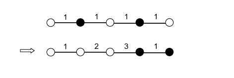
Refer to caption
Figure 23: Graph of the T(111)(12)(SU(3))subscriptsuperscript𝑇12111𝑆𝑈3T^{(12)}_{(111)}(SU(3)) quiver SCFT and its separated graph (black dots pushed to the right).

Here we show explicitly how the matrix model of the separated graph is mapped to the matrix model of the quiver theory in an explicit example. We consider the theory with U(1)×U(1)𝑈1𝑈1U(1)\times U(1) gauge group, one bifundamental hypermultiplet and one fundamental hypermultiplet in each U(1)𝑈1U(1) node. The corresponding SCFT deformed by mass and FI parameters is T(111)(12)(SU(3))subscriptsuperscript𝑇12111𝑆𝑈3T^{(12)}_{(111)}(SU(3)) and its graph is shown in figure 23. After moving the black dots to the right of the graph, one obtains the separated graph of figure 23. The matrix model associated to this graph is:

Zseparsubscript𝑍separ\displaystyle Z_{\rm separ} =dσd2σ~d3λ~dλ2.3!e2πi(t1t2)σj2ch(σσ~j)e2πi(t2t3)(σ~1+σ~2)j,k2,3ch(λkσ~j)sh(σ~12)2e2πit3(k3λ~k)j<ksh(λ~jk)absent𝑑𝜎superscript𝑑2~𝜎superscript𝑑3~𝜆𝑑𝜆2.3superscript𝑒2𝜋𝑖subscript𝑡1subscript𝑡2𝜎superscriptsubscriptproduct𝑗2ch𝜎subscript~𝜎𝑗superscript𝑒2𝜋𝑖subscript𝑡2subscript𝑡3subscript~𝜎1subscript~𝜎2superscriptsubscriptproduct𝑗𝑘23chsubscript𝜆𝑘subscript~𝜎𝑗shsuperscriptsubscript~𝜎122superscript𝑒2𝜋𝑖subscript𝑡3superscriptsubscript𝑘3subscript~𝜆𝑘subscriptproduct𝑗𝑘shsubscript~𝜆𝑗𝑘\displaystyle=\int\frac{d\sigma d^{2}\widetilde{\sigma}d^{3}\widetilde{\lambda}d\lambda}{2.3!}\,\frac{e^{2\pi i(t_{1}-t_{2})\sigma}}{\prod_{j}^{2}\textrm{ch}(\sigma-\widetilde{\sigma}_{j})}\frac{e^{2\pi i(t_{2}-t_{3})(\widetilde{\sigma}_{1}+\widetilde{\sigma}_{2})}}{\prod_{j,k}^{2,3}\textrm{ch}(\lambda_{k}-\widetilde{\sigma}_{j})}\textrm{sh}(\widetilde{\sigma}_{12})^{2}e^{2\pi it_{3}(\sum_{k}^{3}\widetilde{\lambda}_{k})}\prod_{j<k}\textrm{sh}(\widetilde{\lambda}_{jk})
.(wS3(1)wδ(λ~w(1)λ)ch(λm2+i)δ^[λ~w(2)m2+i2]δ^[λ~w(3)m2i2])δ(λm1)\displaystyle\qquad.\ \left(\sum_{w\in S_{3}}(-1)^{w}\frac{\delta(\widetilde{\lambda}_{w(1)}-\lambda)}{\textrm{ch}(\lambda-m_{2}+i)}\hat{\delta}[\widetilde{\lambda}_{w(2)}-m_{2}+\frac{i}{2}]\hat{\delta}[\widetilde{\lambda}_{w(3)}-m_{2}-\frac{i}{2}]\right)\delta(\lambda-m_{1})

After a few simplifications the matrix model can be expressed as

=e2πit3m12ch(m1m2)𝑑σd2σ~d2λ~e2πi(t1t2)σj2ch(σσ~j)e2πi(t2t3)(σ~1+σ~2)j,k2,2ch(λkσ~j)sh(σ~12)2e2πit3(λ~1+λ~2)j2ch(m1σ~j)absentsuperscript𝑒2𝜋𝑖subscript𝑡3subscript𝑚12chsubscript𝑚1subscript𝑚2differential-d𝜎superscript𝑑2~𝜎superscript𝑑2~𝜆superscript𝑒2𝜋𝑖subscript𝑡1subscript𝑡2𝜎superscriptsubscriptproduct𝑗2ch𝜎subscript~𝜎𝑗superscript𝑒2𝜋𝑖subscript𝑡2subscript𝑡3subscript~𝜎1subscript~𝜎2superscriptsubscriptproduct𝑗𝑘22chsubscript𝜆𝑘subscript~𝜎𝑗shsuperscriptsubscript~𝜎122superscript𝑒2𝜋𝑖subscript𝑡3subscript~𝜆1subscript~𝜆2superscriptsubscriptproduct𝑗2chsubscript𝑚1subscript~𝜎𝑗\displaystyle=\frac{e^{2\pi it_{3}m_{1}}}{2\textrm{ch}(m_{1}-m_{2})}\int d\sigma d^{2}\widetilde{\sigma}d^{2}\widetilde{\lambda}\,\frac{e^{2\pi i(t_{1}-t_{2})\sigma}}{\prod_{j}^{2}\textrm{ch}(\sigma-\widetilde{\sigma}_{j})}\frac{e^{2\pi i(t_{2}-t_{3})(\widetilde{\sigma}_{1}+\widetilde{\sigma}_{2})}}{\prod_{j,k}^{2,2}\textrm{ch}(\lambda_{k}-\widetilde{\sigma}_{j})}\frac{\textrm{sh}(\widetilde{\sigma}_{12})^{2}e^{2\pi it_{3}(\widetilde{\lambda}_{1}+\widetilde{\lambda}_{2})}}{\prod_{j}^{2}\textrm{ch}(m_{1}-\widetilde{\sigma}_{j})}
.sh(λ~1λ~2)sh(m1λ~1)sh(m1λ~2)δ^[λ~2m2+i2]δ^[λ~1m2i2].\displaystyle\qquad.\ \textrm{sh}(\widetilde{\lambda}_{1}-\widetilde{\lambda}_{2})\textrm{sh}(m_{1}-\widetilde{\lambda}_{1})\textrm{sh}(m_{1}-\widetilde{\lambda}_{2})\hat{\delta}[\widetilde{\lambda}_{2}-m_{2}+\frac{i}{2}]\hat{\delta}[\widetilde{\lambda}_{1}-m_{2}-\frac{i}{2}]\ .

Integrating over λ~1subscript~𝜆1\widetilde{\lambda}_{1} with the δ^^𝛿\hat{\delta} distribution yields after simplifications (contributions appear from the poles at λ~1=σj+i2subscript~𝜆1subscript𝜎𝑗𝑖2\widetilde{\lambda}_{1}=\sigma_{j}+\frac{i}{2}):

=e2πit3(m1+m2+i2)2𝑑σd2σ~𝑑λ~2e2πi(t1t2)σj2ch(σσ~j)e2πi(t2t3)(σ~1+σ~2)j2ch(λ2σ~j)sh(σ~12)2e2πit3λ~2j2ch(m1σ~j)sh(m1λ~2)absentsuperscript𝑒2𝜋𝑖subscript𝑡3subscript𝑚1subscript𝑚2𝑖22differential-d𝜎superscript𝑑2~𝜎differential-dsubscript~𝜆2superscript𝑒2𝜋𝑖subscript𝑡1subscript𝑡2𝜎superscriptsubscriptproduct𝑗2ch𝜎subscript~𝜎𝑗superscript𝑒2𝜋𝑖subscript𝑡2subscript𝑡3subscript~𝜎1subscript~𝜎2superscriptsubscriptproduct𝑗2chsubscript𝜆2subscript~𝜎𝑗shsuperscriptsubscript~𝜎122superscript𝑒2𝜋𝑖subscript𝑡3subscript~𝜆2superscriptsubscriptproduct𝑗2chsubscript𝑚1subscript~𝜎𝑗shsubscript𝑚1subscript~𝜆2\displaystyle=\frac{e^{2\pi it_{3}(m_{1}+m_{2}+\frac{i}{2})}}{2}\int d\sigma d^{2}\widetilde{\sigma}d\widetilde{\lambda}_{2}\,\frac{e^{2\pi i(t_{1}-t_{2})\sigma}}{\prod_{j}^{2}\textrm{ch}(\sigma-\widetilde{\sigma}_{j})}\frac{e^{2\pi i(t_{2}-t_{3})(\widetilde{\sigma}_{1}+\widetilde{\sigma}_{2})}}{\prod_{j}^{2}\textrm{ch}(\lambda_{2}-\widetilde{\sigma}_{j})}\frac{\textrm{sh}(\widetilde{\sigma}_{12})^{2}e^{2\pi it_{3}\widetilde{\lambda}_{2}}}{\prod_{j}^{2}\textrm{ch}(m_{1}-\widetilde{\sigma}_{j})}\textrm{sh}(m_{1}-\widetilde{\lambda}_{2})
.ch(m2λ~2)δ^[λ~2m2+i2](1sh(σ~1m2)sh(σ~2m2)+i2j=1,2(1)jδ(σ~jm2)sh(σ~12)).\displaystyle\quad.\ \textrm{ch}(m_{2}-\widetilde{\lambda}_{2})\hat{\delta}[\widetilde{\lambda}_{2}-m_{2}+\frac{i}{2}]\ \left(\frac{1}{\textrm{sh}(\widetilde{\sigma}_{1}-m_{2})\textrm{sh}(\widetilde{\sigma}_{2}-m_{2})}+\frac{i}{2}\sum_{j=1,2}(-1)^{j}\frac{\delta(\widetilde{\sigma}_{j}-m_{2})}{\textrm{sh}(\widetilde{\sigma}_{12})}\right)\ .

Then the integration over λ~2subscript~𝜆2\widetilde{\lambda}_{2} can be performed using the remaining δ^^𝛿\hat{\delta}. Four terms appear out of which two vanishes and the two others are equal. In total we obtain

=ie2πit3(m1+2m2)𝑑σd2σ~e2πi(t1t2)σj2ch(σσ~j)e2πi(t2t3)(σ~1+σ~2)sh(σ~12)ch(σ~1m1)sh(σ~1m2)δ(σ~2m2)absent𝑖superscript𝑒2𝜋𝑖subscript𝑡3subscript𝑚12subscript𝑚2differential-d𝜎superscript𝑑2~𝜎superscript𝑒2𝜋𝑖subscript𝑡1subscript𝑡2𝜎superscriptsubscriptproduct𝑗2ch𝜎subscript~𝜎𝑗superscript𝑒2𝜋𝑖subscript𝑡2subscript𝑡3subscript~𝜎1subscript~𝜎2shsubscript~𝜎12chsubscript~𝜎1subscript𝑚1shsubscript~𝜎1subscript𝑚2𝛿subscript~𝜎2subscript𝑚2\displaystyle=i\,e^{2\pi it_{3}(m_{1}+2m_{2})}\int d\sigma d^{2}\widetilde{\sigma}\,\frac{e^{2\pi i(t_{1}-t_{2})\sigma}}{\prod_{j}^{2}\textrm{ch}(\sigma-\widetilde{\sigma}_{j})}e^{2\pi i(t_{2}-t_{3})(\widetilde{\sigma}_{1}+\widetilde{\sigma}_{2})}\frac{\textrm{sh}(\widetilde{\sigma}_{12})}{\textrm{ch}(\widetilde{\sigma}_{1}-m_{1})\textrm{sh}(\widetilde{\sigma}_{1}-m_{2})}\delta(\widetilde{\sigma}_{2}-m_{2})
=ie2πi[t2m2+t3(m1+m2)]𝑑σ𝑑σ~e2πi(t1t2)σch(σm2)ch(σσ~)e2πi(t2t3)σ~ch(σ~m1)absent𝑖superscript𝑒2𝜋𝑖delimited-[]subscript𝑡2subscript𝑚2subscript𝑡3subscript𝑚1subscript𝑚2differential-d𝜎differential-d~𝜎superscript𝑒2𝜋𝑖subscript𝑡1subscript𝑡2𝜎ch𝜎subscript𝑚2ch𝜎~𝜎superscript𝑒2𝜋𝑖subscript𝑡2subscript𝑡3~𝜎ch~𝜎subscript𝑚1\displaystyle=i\,e^{2\pi i[t_{2}m_{2}+t_{3}(m_{1}+m_{2})]}\int d\sigma d\widetilde{\sigma}\,\frac{e^{2\pi i(t_{1}-t_{2})\sigma}}{\textrm{ch}(\sigma-m_{2})\textrm{ch}(\sigma-\widetilde{\sigma})}\frac{e^{2\pi i(t_{2}-t_{3})\widetilde{\sigma}}}{\textrm{ch}(\widetilde{\sigma}-m_{1})}
=ie2πi[t2m2+t3(m1+m2)]Zquiver.absent𝑖superscript𝑒2𝜋𝑖delimited-[]subscript𝑡2subscript𝑚2subscript𝑡3subscript𝑚1subscript𝑚2subscript𝑍quiver\displaystyle=i\,e^{2\pi i[t_{2}m_{2}+t_{3}(m_{1}+m_{2})]}\ Z_{\rm quiver}\ .

As expected, we recover the matrix model for the partition function of the quiver theory we started with. The extra phase is also as expected from (5.8) (as usual we ignore overall factors of i𝑖i).

References

  • [1] K. A. Intriligator and N. Seiberg, Mirror symmetry in three-dimensional gauge theories, Phys.Lett. B387 (1996) 513–519, [hep-th/9607207].
  • [2] J. de Boer, K. Hori, H. Ooguri, and Y. Oz, Mirror symmetry in three-dimensional gauge theories, quivers and D-branes, Nucl.Phys. B493 (1997) 101–147, [hep-th/9611063].
  • [3] J. de Boer, K. Hori, H. Ooguri, Y. Oz, and Z. Yin, Mirror symmetry in three-dimensional theories, SL(2,Z) and D-brane moduli spaces, Nucl.Phys. B493 (1997) 148–176, [hep-th/9612131].
  • [4] A. Hanany and E. Witten, Type IIB superstrings, BPS monopoles, and three-dimensional gauge dynamics, Nucl.Phys. B492 (1997) 152–190, [hep-th/9611230].
  • [5] A. Kapustin, B. Willett, and I. Yaakov, Exact Results for Wilson Loops in Superconformal Chern-Simons Theories with Matter, JHEP 1003 (2010) 089, [arXiv:0909.4559].
  • [6] M. Marino, Lectures on localization and matrix models in supersymmetric Chern-Simons-matter theories, J.Phys. A44 (2011) 463001, [arXiv:1104.0783].
  • [7] A. Kapustin, B. Willett, and I. Yaakov, Nonperturbative Tests of Three-Dimensional Dualities, JHEP 1010 (2010) 013, [arXiv:1003.5694].
  • [8] A. Dey, On Three-Dimensional Mirror Symmetry, JHEP 1204 (2012) 051, [arXiv:1109.0407].
  • [9] A. Dey and J. Distler, Three Dimensional Mirror Symmetry and Partition Function on S3superscript𝑆3S^{3}, arXiv:1301.1731.
  • [10] A. Dey, Mirror Symmetry in Flavored Affine D-type Quivers, arXiv:1401.6462.
  • [11] A. Hanany and N. Mekareeya, Complete Intersection Moduli Spaces in N=4 Gauge Theories in Three Dimensions, JHEP 1201 (2012) 079, [arXiv:1110.6203].
  • [12] S. Cremonesi, A. Hanany, and A. Zaffaroni, Monopole operators and Hilbert series of Coulomb branches of 3d3𝑑3d 𝒩=4𝒩4\mathcal{N}=4 gauge theories, JHEP 1401 (2014) 005, [arXiv:1309.2657].
  • [13] S. Cremonesi, A. Hanany, N. Mekareeya, and A. Zaffaroni, Coulomb branch Hilbert series and Three Dimensional Sicilian Theories, arXiv:1403.2384.
  • [14] S. Cremonesi, A. Hanany, N. Mekareeya, and A. Zaffaroni, Coulomb branch Hilbert series and Hall-Littlewood polynomials, arXiv:1403.0585.
  • [15] A. Dey, A. Hanany, P. Koroteev, and N. Mekareeya, Mirror Symmetry in Three Dimensions via Gauged Linear Quivers, arXiv:1402.0016.
  • [16] E. Witten, SL(2,Z) action on three-dimensional conformal field theories with Abelian symmetry, hep-th/0307041.
  • [17] D. L. Jafferis and X. Yin, Chern-Simons-Matter Theory and Mirror Symmetry, arXiv:0810.1243.
  • [18] D. Gaiotto and E. Witten, Janus Configurations, Chern-Simons Couplings, And The theta-Angle in N=4 Super Yang-Mills Theory, JHEP 1006 (2010) 097, [arXiv:0804.2907].
  • [19] K. Hosomichi, K.-M. Lee, S. Lee, S. Lee, and J. Park, N=4 Superconformal Chern-Simons Theories with Hyper and Twisted Hyper Multiplets, JHEP 0807 (2008) 091, [arXiv:0805.3662].
  • [20] Y. Imamura and K. Kimura, On the moduli space of elliptic Maxwell-Chern-Simons theories, Prog.Theor.Phys. 120 (2008) 509–523, [arXiv:0806.3727].
  • [21] O. Aharony, O. Bergman, D. L. Jafferis, and J. Maldacena, N=6 superconformal Chern-Simons-matter theories, M2-branes and their gravity duals, JHEP 0810 (2008) 091, [arXiv:0806.1218].
  • [22] O. Aharony, O. Bergman, and D. L. Jafferis, Fractional M2-branes, JHEP 0811 (2008) 043, [arXiv:0807.4924].
  • [23] D. Gaiotto and E. Witten, S-Duality of Boundary Conditions In N=4 Super Yang-Mills Theory, arXiv:0807.3720.
  • [24] Y. Imamura and K. Kimura, N=4 Chern-Simons theories with auxiliary vector multiplets, JHEP 0810 (2008) 040, [arXiv:0807.2144].
  • [25] D. R. Gulotta, C. P. Herzog, and S. S. Pufu, From Necklace Quivers to the F-theorem, Operator Counting, and T(U(N)), arXiv:1105.2817.
  • [26] T. Nishioka, Y. Tachikawa, and M. Yamazaki, 3d Partition Function as Overlap of Wavefunctions, JHEP 1108 (2011) 003, [arXiv:1105.4390].
  • [27] C. Closset, T. T. Dumitrescu, G. Festuccia, Z. Komargodski, and N. Seiberg, Contact Terms, Unitarity, and F-Maximization in Three-Dimensional Superconformal Theories, JHEP 1210 (2012) 053, [arXiv:1205.4142].
  • [28] C. Closset, T. T. Dumitrescu, G. Festuccia, Z. Komargodski, and N. Seiberg, Comments on Chern-Simons Contact Terms in Three Dimensions, JHEP 1209 (2012) 091, [arXiv:1206.5218].
  • [29] B. Assel, C. Bachas, J. Estes, and J. Gomis, Holographic Duals of D=3 N=4 Superconformal Field Theories, JHEP 1108 (2011) 087, [arXiv:1106.4253].
  • [30] B. Assel, C. Bachas, J. Estes, and J. Gomis, IIB Duals of D=3 N=4 Circular Quivers, JHEP 1212 (2012) 044, [arXiv:1210.2590].
  • [31] O. Aharony, A. Hanany, K. A. Intriligator, N. Seiberg, and M. Strassler, Aspects of N=2 supersymmetric gauge theories in three-dimensions, Nucl.Phys. B499 (1997) 67–99, [hep-th/9703110].
  • [32] D. Gaiotto and X. Yin, Notes on superconformal Chern-Simons-Matter theories, JHEP 0708 (2007) 056, [arXiv:0704.3740].
  • [33] T. Kitao, K. Ohta, and N. Ohta, Three-dimensional gauge dynamics from brane configurations with (p,q) - five-brane, Nucl.Phys. B539 (1999) 79–106, [hep-th/9808111].
  • [34] Y. Imamura and S. Yokoyama, N=4 Chern-Simons theories and wrapped M-branes in their gravity duals, Prog.Theor.Phys. 121 (2009) 915–940, [arXiv:0812.1331].
  • [35] S. Benvenuti and S. Pasquetti, 3D-partition functions on the sphere: exact evaluation and mirror symmetry, arXiv:1105.2551.
  • [36] F. V. de Bult, Hyperbolic hypergeometric functions, University of Amsterdam PhD thesis (2007).
  • [37] O. Bergman, A. Hanany, A. Karch, and B. Kol, Branes and supersymmetry breaking in three-dimensional gauge theories, JHEP 9910 (1999) 036, [hep-th/9908075].
  • [38] A. Hanany and D. Tong, Vortices, instantons and branes, JHEP 0307 (2003) 037, [hep-th/0306150].
  • [39] A. Giveon and D. Kutasov, Seiberg Duality in Chern-Simons Theory, Nucl.Phys. B812 (2009) 1–11, [arXiv:0808.0360].
  • [40] A. Kapustin, B. Willett, and I. Yaakov, Tests of Seiberg-like Duality in Three Dimensions, arXiv:1012.4021.
  • [41] S. Matsumoto and S. Moriyama, ABJ Fractional Brane from ABJM Wilson Loop, arXiv:1310.8051.