Magnetic and Ising quantum phase transitions in a model for isoelectronically tuned iron pnictides

Abstract

Considerations of the observed bad-metal behavior in Fe-based superconductors led to an early proposal for quantum criticality induced by isoelectronic P for As doping in iron arsenides, which has since been experimentally confirmed. We study here an effective model for the isoelectronically tuned pnictides using a large-$N$ approach. The model contains antiferromagnetic and Ising-nematic order parameters appropriate for $J_{1}$-$J_{2}$ exchange-coupled local moments on an Fe square lattice, and a damping caused by coupling to itinerant electrons. The zero-temperature magnetic and Ising transitions are concurrent and essentially continuous. The order-parameter jumps are very small, and are further reduced by the inter-plane coupling; consequently, quantum criticality occurs over a wide dynamical range. Our results reconcile recent seemingly contradictory experimental observations concerning the quantum phase transition in the P-doped iron arsenides.

Introduction.

Iron pnictide and chalcogenide materials not only show high-temperature superconductivity kamihara , but also feature rich phase diagrams. For the undoped parent iron arsenides, the ground state has collinear $(\pi,0)$ magnetic order delaCruz . Because superconductivity occurs at the border of this antiferromagnetic (AF) order, a natural question is whether quantum criticality plays a role in the phase diagram. Early on, it was proposed theoretically that tuning the parent iron arsenide by isoelectronic P-for-As doping induces quantum criticality associated with the suppression of both the $(\pi,0)$ AF order and an Ising-nematic spin order dai . This proposal was made within a strong-coupling approach, which attributes the bad-metal behavior of iron arsenides qazilbash ; hu ; degiorgi ; nakajima to correlation effects that are on the verge of localizing electrons si ; si2 ; kotliar2 along with their associated magnetic moments. The P doping increases the in-plane electronic kinetic energy (as P is smaller than As), and thus the coherent electronic spectral weight while leaving other model parameters little changed quebe ; zimmer . This weakens both the magnetic order and the associated Ising-nematic spin order dai ; abrahams .

Experimental evidence for a quantum critical point (QCP) has since emerged in the P-doped CeFeAsO cruz ; luo and P-doped BaFe₂As₂ kasahara ; nakai ; hashimoto ; analytis ; analytis2 . In the phase diagram of the P-doped BaFe₂As₂, an extended temperature and doping regime has been identified for non-Fermi liquid behavior kasahara ; nakai ; hashimoto ; analytis . An Ising-nematic order, inferred from the tetragonal-to-orthorhombic structural distortion, is suppressed around the same P-doping concentration ($x_{c}\approx 0.33$) at which the AF order disappears. While there is evidence for a QCP “hidden” inside the superconducting dome hashimoto , quantum criticality has now been observed and studied in the normal state when superconductivity is suppressed by a high field analytis ; analytis2 . We note that the bad-metal behavior persists through $x_{c}$ kasahara .

Recently, evidence for a weakly first-order nature of the transition has come from the neutron-scattering experiments in the P-doped BaFe₂As₂ DHu . It is in seeming contradiction with the accumulated experimental evidence for quantum criticality. This puzzle calls for further theoretical analyses on the underlying quantum phase transitions. More generally, the interplay between the magnetic and nematic orders exemplifies the kind of competing or coexisting orders that is of general interest to a variety of strongly correlated electron systems.

In this letter, we study the zero-temperature phase transitions in the appropriate effective Ginzburg-Landau field theory that was introduced earlier dai ; abrahams to describe the low-energy properties of a $J_{1}$-$J_{2}$ model of local moments on a square lattice coupled to coherent itinerant electrons dai ; chandra ; si ; fang ; xu . The theory contains antiferromagnetic (vector) and Ising-nematic (scalar) order parameters as well as a damping term. Since it is important to establish the nature of quantum criticality in the absence of superconductivity cruz ; analytis ; analytis2 , we will focus on the transitions in the normal state and will not consider the effect of superconductivity fernandes . Using a large-$N$ approach rancon ; sidney-coleman , we demonstrate that the AF and Ising-nematic transitions are concurrent at zero temperature both for the case of a square lattice and in the presence of interlayer coupling. Moreover, both transitions are only weakly first order in accordance with the marginal nature of the relevant coupling, with jumps in both order parameters that are very small, which implies a large dynamical range for quantum criticality. Our results provide a natural resolution to the aforementioned puzzle.

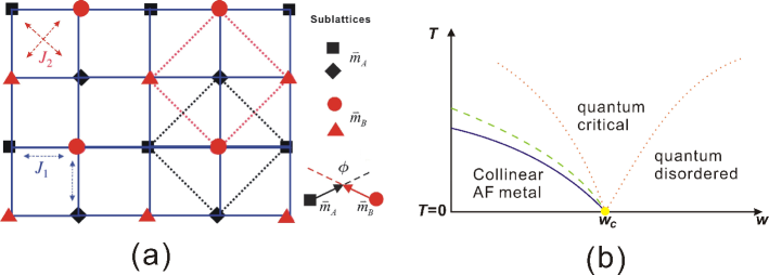
Figure 1: (a) Illustration of the $J_{1}-J_{2}$ model on a square lattice. The staggered magnetizations $\overset{\lower 5.0pt\hbox{$\smash{\scriptscriptstyle\rightharpoonup}$}}{m}_{A}$ and $\overset{\lower 5.0pt\hbox{$\smash{\scriptscriptstyle\rightharpoonup}$}}{m}_{B}$ are defined on two interpenetrating Néel square lattices; (b) Schematic phase diagram proposed for the P-doped iron arsenides dai . P-doping increases $w$, the spectral weight of the coherent itinerant electrons. The yellow dot denotes the tuning parameter $w_{c}$ for the QCP. The purple solid line and the green dashed one respectively mark the AF and structural transitions.

The model.

The proximity of a bad metal to a Mott transition can be measured by a parameter $w$, the percentage of the single-electron spectral weight in the coherent itinerant part dai ; si ; si2 ; moeller . This approach has been successful in describing the spin excitation spectrum of the iron pnictides yu ; pallab ; Diallo2010 ; Harriger2011 , and in understanding the fact that $T_{c}$ in the iron-based superconductors with purely electron Fermi pockets is at least comparably high compared with those with nested Fermi surfaces of co-existing hole and electron pockets RYu2013a ; JGuo2010 ; Fang2011 ; Xue.2012 ; SLHe2013 ; Shen.2014 ; YWang2015 . At the zeroth order in $w$, all the single-electron excitations are incoherent; integrating out the corresponding charge excitations leads to couplings $J_{1}$ and $J_{2}$ among the residual local moments:

$$H=\sum\limits_{\left\langle{i,j}\right\rangle}{J_{1}\overset{\lower 5.0pt\hbox{$\smash{\scriptscriptstyle\rightharpoonup}$}}{S}_{i}\cdot\overset{\lower 5.0pt\hbox{$\smash{\scriptscriptstyle\rightharpoonup}$}}{S}_{j}}+\sum\limits_{\left\langle{\left\langle{i,j}\right\rangle}\right\rangle}{J_{2}\overset{\lower 5.0pt\hbox{$\smash{\scriptscriptstyle\rightharpoonup}$}}{S}_{i}\cdot\overset{\lower 5.0pt\hbox{$\smash{\scriptscriptstyle\rightharpoonup}$}}{S}_{j}}$$ (1)

where $\left\langle{\cdots}\right\rangle$ and $\left\langle{\left\langle\cdots\right\rangle}\right\rangle$ respectively denote the nearest neighbor and next nearest neighbor sites; see Fig. 1(a). Both general considerations si and first-principal calculations yildirim ; ma suggest that $J_{2}>J_{1}/2$. In this regime, we consider two interpenetrating sublattices [the dotted squares in Fig. 1(a)], having independent staggered magnetizations with Néel vectors $\overset{\lower 5.0pt\hbox{$\smash{\scriptscriptstyle\rightharpoonup}$}}{m}_{A}$ and $\overset{\lower 5.0pt\hbox{$\smash{\scriptscriptstyle\rightharpoonup}$}}{m}_{B}$. While the mean-field energy is independent of the angle $\phi$ between $\overset{\lower 5.0pt\hbox{$\smash{\scriptscriptstyle\rightharpoonup}$}}{m}_{A}$ and $\overset{\lower 5.0pt\hbox{$\smash{\scriptscriptstyle\rightharpoonup}$}}{m}_{B}$, this degeneracy is broken by quantum or thermal fluctuations. It leads to the collinear order with $\phi=0$ or $\pi$ henley ; chandra . Thus $\overset{\lower 5.0pt\hbox{$\smash{\scriptscriptstyle\rightharpoonup}$}}{m}_{A}\cdot\overset{\lower 5.0pt\hbox{$\smash{\scriptscriptstyle\rightharpoonup}$}}{m}_{B}=\pm 1$ becomes an Ising variable.

At non-vanishing orders in $w$, the coherent itinerant electrons provide Landau damping. This leads to the following Ginzburg-Landau action dai ; abrahams :

$$S=S_{2}+S_{4}$$ (2)

with

$$\begin{gathered}S_{2}=\sum\limits_{\overset{\lower 3.5pt\hbox{$\smash{\scriptscriptstyle\rightharpoonup}$}}{q},i\omega_{l}}{\left\{{\chi_{0}^{-1}(\overset{\lower 5.0pt\hbox{$\smash{\scriptscriptstyle\rightharpoonup}$}}{q},i\omega_{l})\left[{\left|{\overset{\lower 5.0pt\hbox{$\smash{\scriptscriptstyle\rightharpoonup}$}}{m}_{A}(\overset{\lower 5.0pt\hbox{$\smash{\scriptscriptstyle\rightharpoonup}$}}{q},i\omega_{l})}\right|^{2}+\left|{\overset{\lower 5.0pt\hbox{$\smash{\scriptscriptstyle\rightharpoonup}$}}{m}_{B}(\overset{\lower 5.0pt\hbox{$\smash{\scriptscriptstyle\rightharpoonup}$}}{q},i\omega_{l})}\right|^{2}}\right]+2v\left({q_{x}^{2}-q_{y}^{2}}\right)\overset{\lower 5.0pt\hbox{$\smash{\scriptscriptstyle\rightharpoonup}$}}{m}_{A}(\overset{\lower 5.0pt\hbox{$\smash{\scriptscriptstyle\rightharpoonup}$}}{q},i\omega_{l})\cdot\overset{\lower 5.0pt\hbox{$\smash{\scriptscriptstyle\rightharpoonup}$}}{m}_{B}(-\overset{\lower 5.0pt\hbox{$\smash{\scriptscriptstyle\rightharpoonup}$}}{q},-i\omega_{l})}\right\}},\hfill\\ S_{4}=\int_{0}^{\beta}{d\tau\int{d\overset{\lower 5.0pt\hbox{$\smash{\scriptscriptstyle\rightharpoonup}$}}{r}\left\{{u_{1}\left({\left|{\overset{\lower 5.0pt\hbox{$\smash{\scriptscriptstyle\rightharpoonup}$}}{m}_{A}}\right|^{4}+\left|{\overset{\lower 5.0pt\hbox{$\smash{\scriptscriptstyle\rightharpoonup}$}}{m}_{B}}\right|^{4}}\right)+u_{2}\left|{\overset{\lower 5.0pt\hbox{$\smash{\scriptscriptstyle\rightharpoonup}$}}{m}_{A}}\right|^{2}\left|{\overset{\lower 5.0pt\hbox{$\smash{\scriptscriptstyle\rightharpoonup}$}}{m}_{B}}\right|^{2}-u_{I}\left({\overset{\lower 5.0pt\hbox{$\smash{\scriptscriptstyle\rightharpoonup}$}}{m}_{A}\cdot\overset{\lower 5.0pt\hbox{$\smash{\scriptscriptstyle\rightharpoonup}$}}{m}_{B}}\right)^{2}}\right\}}}.\hfill\\ \end{gathered}$$ (3)

The ${\vec{m}}_{A/B}$ are in either momentum and Matsubara frequency space ($S_{2}$) or real space and imaginary time ($S_{4}$). In $S_{2}$, the inverse susceptibility is

$$\chi_{0}^{-1}(\mathord{\buildrel{\lower 3.0pt\hbox{$\scriptscriptstyle\rightharpoonup$}}\over{q}},i\omega_{l})=r+\omega_{l}^{2}+c~{}q^{2}+\gamma\left|{\omega_{l}}\right|,$$ (4)

where $c$ is the square of the spin-wave velocity and in $S_{4}$, the coupling $u_{I}>0$ dai ; chandra . The parameter $v$ leads to the anisotropic distribution of the spin spectral weight in momentum space, which is observed in neutron scattering Diallo2010 ; Harriger2011 . It is described by the ellipticity

$$\epsilon\equiv\sqrt{(c-v)/(c+v)},$$ (5)

which goes from full isotropy $\epsilon=1$ ($v=0$) to extreme anisotropy $\epsilon=0$ ($v=c$). In addition, $\gamma$ is the (Landau) damping rate and $r=r_{0}+wA_{\bf Q}$, where $r_{0}$ is negative, reflecting ground-state order in the absence of damping, and $A_{\bf Q}>0$ is related to a quasiparticle susceptibility at ${\bf Q}=(\pi,0)$ or $(0,\pi)$ dai . The mass $r$ vanishes at $w=w_{c}$, the point of quantum phase transition. When the damping is present, the effective dimensionality of the fluctuations is $d+z=4$. From a renormalization-group (RG) perspective, because “$-u_{I}$” is negative, it is marginally relevant w.r.t the underlying QCP at $d+z=4$ dai ; qi . So unlike thermally-driven transitions or the case of a zero-temperature transition in the absence of damping (where $u_{I}$ is relevant), the marginal nature of the coupling is expected to yield only a small change to the underlying QCP; this leads to a qualitative phase diagram shown in Fig. 1(b) dai ; abrahams .

Given the aforementioned experimental observations, we shall study the phase transitions beyond qualitative RG-based considerations. Our focus is on the zero-temperature limit, and we place particular emphasis on the effect of damping. We note that the effect of damping on the transitions and dynamics at non-zero temperatures has been studied before pallab . The action $S$ is a functional of the (vector) magnetization fields ${\vec{m}}_{A/B}$ and we may derive the free-energy density from ${\cal F}=-\ln\int{\cal D}\{m\}\exp(-S(\{m\})$.

Large-$N$ approach.—

To study the phase transitions for the two-sublattice action of Eq. (3) beyond mean-field theory, we generalize the spin symmetry of the model to $O(N)$ (${\vec{m}}_{A/B}$ will have $N$ components) and study it through a $1/N$ expansion. Our goal is to investigate general properties, including issues of universality and the order of the phase transitions of the present setting, which contains two order parameters possibly competing or coexisting. We note that the well-known large-$N$ approach has proved fruitful for many problems in statistical physics rancon ; sidney-coleman .

To proceed, we rescale the quartic couplings in $S(\{m\})$ by a factor $1/N$ and in the functional integral over $e^{-S}$ for ${\cal F}$, we decompose them in terms of Hubbard-Stratonovich fields $\lambda_{A/B}$ and $\Delta_{I}.$ For details, refer to the Supplementary Material (SM) supplemental . To leading order in $1/N$, $i\lambda_{A/B}=\langle m_{A/B}^{2}\rangle\equiv m^{2}$ contribute to the renormalization of the mass (coefficient of the quadratic term in the action $S_{2}$) and $\;\Delta_{I}=\left\langle{\mathord{\buildrel{\lower 3.0pt\hbox{$\scriptscriptstyle\rightharpoonup$}}\over{m}}_{A}\cdot\mathord{\buildrel{\lower 3.0pt\hbox{$\scriptscriptstyle\rightharpoonup$}}\over{m}}_{B}}\right\rangle$ is the Ising order parameter. We carry out our analysis from the ordered side, and set $\mathord{\buildrel{\lower 3.0pt\hbox{$\scriptscriptstyle\rightharpoonup$}}\over{m}}_{A/B}=\left({\sqrt{N}\sigma_{A/B},\mathord{\buildrel{\lower 3.0pt\hbox{$\scriptscriptstyle\rightharpoonup$}}\over{\pi}}_{A/B}}\right)$ with ${\sigma_{A/B}}$ and ${\mathord{\buildrel{\lower 3.0pt\hbox{$\scriptscriptstyle\rightharpoonup$}}\over{\pi}}_{A/B}}$ as the static order and fluctuation fields of sublattices $A$ and $B$ respectively. To order $O(1/N)$ we can integrate out ${\mathord{\buildrel\lower 3.0pt\hbox{$\scriptscriptstyle\rightharpoonup$}\over{\pi}}_{A/B}}$, which yields an effective free energy density ${\cal F}(\sigma,m^{2},\Delta_{I})$ that depends parametrically on the damping strength $\gamma$, the square of the spin-wave velocity $c$, the anisotropy parameter $v$, and the quartic coupling constants $u_{I},2u_{1}+u_{2}$. From SM, Eqs. (S6,S7), we have the free energy density

$${\cal F}=\frac{\Delta_{I}^{2}}{u_{I}}-\frac{(m^{2}-r)^{2}}{2u_{1}+u_{2}}+(m^{2}\pm\Delta_{I})\sigma^{2}+g(m^{2},\Delta_{I})$$ (6)

with

$$g(m^{2},\Delta_{I}) =\frac{1}{2\beta V}\sum_{{\vec{q}},l}\ln\big{\{}(D_{0,{\vec{q}},l}^{-1}+m^{2})^{2}$$

$$-[v(q_{x}^{2}-q_{y}^{2})+\Delta_{I}]^{2}\big{\}},$$ (7)

where $D_{0,{\vec{q}},l}^{-1}=\chi^{-1}_{0,{\vec{q}},l}-r$, containing $\gamma$, see Eq. (4). The two cases $\sigma_{A}=\sigma_{B}=\sigma$ ($+$sign in Eq. (6)) and $\sigma_{A}=-\sigma_{B}=\sigma$ ($-$sign) correspond to ${\bf{Q}}=(0,\pi)$ and $(\pi,0)$) AF orders, respectively.

Then we have variational equations w.r.t $\sigma$, $m^{2}$ and $\Delta_{I}$,

$$\frac{{\partial{\cal F}}}{{\partial\sigma}}=\frac{{\partial{\cal F}}}{{\partial\Delta_{I}}}=\frac{{\partial{\cal F}}}{{\partial m^{2}}}=0$$ (8)

which in turn correspond to [see SM, Eqs. (S9-S11)] supplemental

$$\left({m^{2}-|\Delta_{I}|}\right)\sigma=0,$$ (9)

$$\frac{{\Delta_{I}}}{{u_{I}}} =\frac{{m^{2}-r}}{{2u_{1}+u_{2}}}-2\sigma^{2}-G_{+},$$ (10)

$$\frac{{\Delta_{I}}}{{u_{I}}} =-\frac{{m^{2}-r}}{{2u_{1}+u_{2}}}+G_{-}.$$ (11)

Here $G_{\pm}$ are given by

$$G_{\pm}=\frac{1}{2\beta V}\sum_{{\vec{q}},l}\frac{1}{D_{0,{\vec{q}},l}^{-1}\pm v(q_{x}^{2}-q_{y}^{2})+m^{2}\pm\Delta_{I}}.$$ (12)

Several limits provide a check on our approach. From Eqs. (10,11), setting $u_{I}=0$ will lead to $\Delta_{I}=0$; this is consistent with the Ising order being driven by the interaction $u_{I}$. In the absence of coupling to coherent itinerant fermions i.e., setting $\gamma^{2}/|\Delta_{I}|=0$ and $w=0$, we have a nonzero Ising order at zero temperature, which is what happens for the pure $J_{1}-J_{2}$ model henley ; chandra . The detailed analysis of these saddle-point equations is in SM, Eqs.  (S12-S15). It follows that the vanishing of the Ising order implies a vanishing magnetic order. The converse can also be shown explicitly by analyzing Eq. (S15) of the SM, and is numerically confirmed (see below).

Nature of the magnetic and Ising transitions at zero temperature.—

We are now in position to address the concurrent magnetic and Ising transition at $T=0$. The RG argument we described earlier suggests that there will be a jump of the order parameters across the transition, but the jump will be smaller as the damping parameter $\gamma$ increases. To see how the damping affects the transition, we first consider the parameter regime where analytical insights can be gained in our large-$N$ approach. When $\gamma$ is sufficiently large so that $x,y\ll 1$, Eq. (10) simplifies to be supplemental

$$A(\eta)=a\eta-\eta\ln\eta=\mu(w)$$ (13)

with $\eta=|\Delta_{I}|/\gamma^{2}$, and

$$\begin{gathered}a=-\frac{{8\pi^{2}\Gamma\left({a_{I}-a_{0}}\right)}}{{\epsilon+1/\epsilon}}-\ln 2-1/2,\hfill\\ \mu(w)=\frac{{8\pi^{2}a_{0}}}{{(\epsilon+1/\epsilon)\Gamma}}\frac{{r(w)}}{{c\Lambda_{c}^{2}}}+\frac{\tan^{-1}(2/\Gamma)}{{\Gamma}}-\frac{1}{4}\ln(1+\frac{4}{\Gamma^{2}}),\hfill\\ \end{gathered}$$ (17)

where $\Gamma=\frac{\gamma}{{c^{1/2}\Lambda_{c}}}$ is the normalized damping rate, while $a_{0}=\frac{{\Lambda_{c}c^{3/2}}}{{2u_{1}+u_{2}}}$ and $a_{I}=\frac{{\Lambda_{c}c^{3/2}}}{u_{I}}$ relate to the normalized interactions. As described in detail in the Supplementary Material supplemental , it follows from this equation that the transition is first order, with the jump of the order parameter decreasing as the damping rate $\Gamma$ is increased. The jump is exponentially suppressed when $\Gamma$ becomes large.

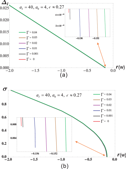
Figure 2: The evolution of the Ising order parameter $\Delta_{I}$ (a) and the collinear AF order parameter $\sigma$ (b) $vs.$ the control parameter at different damping rates ($\Gamma=\gamma/(c^{1/2}\Lambda_{c})$) at a relatively large anisotropy $\epsilon\approx 0.27$, with fixed values of the normalized interactions $a_{I}$ and $a_{0}$. Each order parameter is normalized so that its value deep in the ordered phase is $1$. The transition is very weakly first order, with jumps in the order parameters (insets) that are very small and decrease with damping: already for relatively small damping rate, the jump is on the order of $10^{-6}$ (and $10^{-3}$) for the nematic (and AF) order parameter.

To study the transition more quantitatively, we have solved the large-$N$ equations numerically. Fig. 2 shows how the Ising and magnetic order parameters change when tuning $w$, where, for comparison, we assume $r$ can still be tuned even at $\gamma=0$. The jump of the order parameters is seen to be very small, even for the case of a relatively large anisotropy: of ellipticity $\epsilon\approx 0.27$.

As explained in SM (and verified numerically: compare Fig. 2 and Fig. S2 for a case of extreme anisotropy with $\epsilon\approx 0.025$), the order-parameter jump decreases with decreasing anisotropy (i.e., increasing ellipticity $\epsilon$). Experiments in the iron arsenides observe an ellipticity of $\epsilon\approx 0.7$ pallab ; Diallo2010 , i.e. an anisotropy weaker than that shown in Fig. 2. We then expect even smaller jumps of the order parameters across the quantum phase transition.

Effect of the third-dimensional coupling.—

Iron pnictides have a finite Néel temperature, which results from an interlayer exchange coupling. In order to understand the role of this coupling on the quantum phase transition, we have studied the effective field theory in three-dimensional space. The details of the model are described in the Supplementary Material supplemental , and the results for the case with the spin-wave velocity on the third dimension being equal to the in-plane velocity at $v=0$ are shown in Figs. S3,S4. The AF and Ising transitions are still concurrent, and become genuinely continuous. Again, this is consistent with the RG considerations: given that the effective dimensionality in this case is $d+z=5$, the quartic coupling $-u_{I}$ becomes irrelevant w.r.t. the underlying QCP and will therefore not destabilize the continuous nature of the transition.

In the more general case, with a varying third-dimensional coupling, it is more difficult to solve the large-$N$ equations. However, the RG considerations imply that turning on the interlayer coupling from the purely 2D limit will further suppress the jump in the order parameters.

Discussion.—

Our results imply that the model for the isoelectronically doped iron pnictides yields quantum phase transitions of the AF and Ising-nematic orders that are concurrent, and essentially second order. In other words, while in two-dimensions the transition is eventually first-order, the jumps of the order parameters are small enough to allow a large dynamical range for quantum criticality; the smallness of the jumps is ultimately traced to the marginal nature of the relevant coupling in the effective field theory. In three dimensions, the transition is continuous. Our conclusion reconciles the recent observations of quantum criticality in the normal states of P-doped BaFe₂As₂ analytis ; analytis2 on the one hand, and the neutron-scattering determination of the weakly first order nature of the quantum transition DHu .

In addition, the extremely small jump of the order parameters across the quantum phase transition in the two-dimensional case is also important for understanding other experimental observations. It implies that quantum criticality occurs over a wide dynamical range, with two-dimensional character. The logarithmic divergence of the effective mass expected from such quantum critical fluctuations dai ; abrahams has received considerable experimental support in the P-doped BaFe₂As₂. It fits well the P-doping dependence of the effective mass as extracted from the de Haas-van Alphen (dHvA) measurements shishido , as well as that of the square root of the $T^{2}$-coefficient of the electrical resistivity analytis . Finally, initial dynamical evidence for quantum critical fluctuations in the antiferromagnetic and Ising-nematic channels has come from inelastic neutron scattering measurements in the electron-doped BaFe₂As₂ detwinned by uniaxial strain lu ; song2015 ; it would be very instructive to explore similar effects in the P-doped BaFe₂As₂.

Conclusion.—

We studied zero-temperature magnetic and Ising transitions in a model for isoelectronically tuned iron pnictides using a large-N approach. We demonstrated that the two transitions are concurrent at zero temperature. We also showed that the transition in the presence of damping are essentially continuous; jumps in the order parameters are extremely small, and are further suppressed by an inter-plane coupling. Our results imply the occurrence of quantum criticality in the isoelectronically doped iron pnictides, and reconcile several seemingly contradictory experimental observations in the P-doped iron arsenides.

I Acknowledgement

We thank J. G. Analytis, P. Dai, W. Ding, A. H. Nevidomskyy, J. H. Pixley and Z. Wang for useful discussions. The work has been supported in part by the NSF Grant No. DMR-1309531 and the Robert A. Welch Foundation Grant No. C-1411 (at Rice, J.W. and Q.S.) and by the AFOSR Grant No. FA9550-14-1-0168 (at UCSD, J.W.). Q.S.  acknowledges the support of the Alexander von Humboldt Foundation, and the hospitality of the the Karlsruhe Institute of Technology and the Institute of Physics of Chinese Academy of Sciences.

Supplemental Material – Magnetic and Ising quantum phase transitions in a model for isoelectronically tuned iron pnictides

Jinda Wu, Qimiao Si, and Elihu Abrahams

II Effective Action at Large $N$

The action, from the main text, Eqs. (2,3) is $S(\{m\})=S_{2}+S_{4}$, where

$$S_{2} = \sum\limits_{\overset{\lower 3.5pt\hbox{$\smash{\scriptscriptstyle\rightharpoonup}$}}{q},\omega_{l}}{\left\{{\chi_{0,\overset{\lower 3.5pt\hbox{$\smash{\scriptscriptstyle\rightharpoonup}$}}{q},\omega_{l}}^{-1}\left({\left|{\overset{\lower 5.0pt\hbox{$\smash{\scriptscriptstyle\rightharpoonup}$}}{m}_{A,\overset{\lower 3.5pt\hbox{$\smash{\scriptscriptstyle\rightharpoonup}$}}{q},\omega_{l}}}\right|^{2}+\left|{\overset{\lower 5.0pt\hbox{$\smash{\scriptscriptstyle\rightharpoonup}$}}{m}_{B,\overset{\lower 3.5pt\hbox{$\smash{\scriptscriptstyle\rightharpoonup}$}}{q},\omega_{l}}}\right|^{2}}\right)+2v\left({q_{x}^{2}-q_{y}^{2}}\right)\overset{\lower 5.0pt\hbox{$\smash{\scriptscriptstyle\rightharpoonup}$}}{m}_{A,\overset{\lower 3.5pt\hbox{$\smash{\scriptscriptstyle\rightharpoonup}$}}{q},\omega_{l}}\cdot\overset{\lower 5.0pt\hbox{$\smash{\scriptscriptstyle\rightharpoonup}$}}{m}_{B,-\overset{\lower 3.5pt\hbox{$\smash{\scriptscriptstyle\rightharpoonup}$}}{q},-\omega_{l}}}\right\}}$$ (S1)

$$S_{4} = \int_{0}^{\beta}{d\tau\int{d^{2}\overset{\lower 5.0pt\hbox{$\smash{\scriptscriptstyle\rightharpoonup}$}}{r}\left\{{u_{1}\left[{\left({\overset{\lower 5.0pt\hbox{$\smash{\scriptscriptstyle\rightharpoonup}$}}{m}_{A}^{2}}\right)^{2}+\left({\overset{\lower 5.0pt\hbox{$\smash{\scriptscriptstyle\rightharpoonup}$}}{m}_{B}^{2}}\right)^{2}}\right]+u_{2}\;\overset{\lower 5.0pt\hbox{$\smash{\scriptscriptstyle\rightharpoonup}$}}{m}_{A}^{2}\overset{\lower 5.0pt\hbox{$\smash{\scriptscriptstyle\rightharpoonup}$}}{m}_{B}^{2}-u_{I}\left({\overset{\lower 5.0pt\hbox{$\smash{\scriptscriptstyle\rightharpoonup}$}}{m}_{A}\cdot\overset{\lower 5.0pt\hbox{$\smash{\scriptscriptstyle\rightharpoonup}$}}{m}_{B}}\right)^{2}}\right\}}}$$ (S2)

where the ${\vec{m}}_{A/B}$ are $O(N)$ vector fields of the $A/B$ sublattices in either momentum and Matsubara frequency space ($S_{2}$) or real space and imaginary time ($S_{4}$) and $\chi_{0}^{-1}=r+\omega_{l}^{2}+c~{}q^{2}+\gamma\left|{\omega_{l}}\right|$ with $r=r_{0}+wA_{Q}$. The quartic couplings have been rescaled by a factor $1/N$ and in the functional integral for the free energy ${\cal F}=-\ln\int{\cal D}\{m\}\exp(-S(\{m\})$, they can be decoupled as follows:

$$e^{(u_{I}/N)\int{dx\left({\overset{\lower 3.5pt\hbox{$\smash{\scriptscriptstyle\rightharpoonup}$}}{m}_{A}\cdot\overset{\lower 3.5pt\hbox{$\smash{\scriptscriptstyle\rightharpoonup}$}}{m}_{B}}\right)^{2}}}=L_{1}\int{D\Delta_{I}e^{\int{dx\left({-\frac{{N\Delta_{I}^{2}}}{{u_{I}}}-2\Delta_{I}\overset{\lower 3.5pt\hbox{$\smash{\scriptscriptstyle\rightharpoonup}$}}{m}_{A}\cdot\overset{\lower 3.5pt\hbox{$\smash{\scriptscriptstyle\rightharpoonup}$}}{m}_{B}}\right)}}}$$ (S3)

and

$$e^{-r\sum\limits_{\overset{\lower 2.5pt\hbox{$\smash{\scriptscriptstyle\rightharpoonup}$}}{q},\omega_{l}}{\left({\left|{\overset{\lower 3.5pt\hbox{$\smash{\scriptscriptstyle\rightharpoonup}$}}{m}_{A,\overset{\lower 2.5pt\hbox{$\smash{\scriptscriptstyle\rightharpoonup}$}}{q},\omega_{l}}}\right|^{2}+\left|{\overset{\lower 3.5pt\hbox{$\smash{\scriptscriptstyle\rightharpoonup}$}}{m}_{B,\overset{\lower 2.5pt\hbox{$\smash{\scriptscriptstyle\rightharpoonup}$}}{q},\omega_{l}}}\right|^{2}}\right)-}\int{dx\left\{{(u_{1}/N)\left[{\left({\overset{\lower 3.5pt\hbox{$\smash{\scriptscriptstyle\rightharpoonup}$}}{m}_{A}^{2}}\right)^{2}+\left({\overset{\lower 3.5pt\hbox{$\smash{\scriptscriptstyle\rightharpoonup}$}}{m}_{B}^{2}}\right)^{2}}\right]+(u_{2}/N)\overset{\lower 3.5pt\hbox{$\smash{\scriptscriptstyle\rightharpoonup}$}}{m}_{A}^{2}\overset{\lower 3.5pt\hbox{$\smash{\scriptscriptstyle\rightharpoonup}$}}{m}_{B}^{2}}\right\}}}$$ (S4)

$$=L_{2}\int{D\lambda_{A}D\lambda_{B}e^{-i\lambda_{A}m_{A}^{2}-i\lambda_{B}m_{B}^{2}}e^{\frac{1}{2}\int{dx\left({i\lambda_{A}-r,i\lambda_{B}-r}\right)\frac{{Nu_{1}}}{{4u_{1}^{2}-u_{2}^{2}}}\left({\begin{array}[]{*{20}c}2&{-u_{2}/u_{1}}\\ {-u_{2}/u_{1}}&2\\ \end{array}}\right)\left(\begin{subarray}{l}i\lambda_{A}-r\\ i\lambda_{B}-r\end{subarray}\right)}}}$$ (S7)

with the normalized factors

$$L_{1}=\prod\limits_{x}{\sqrt{\frac{{u_{I}/N}}{\pi}}},\;L_{2}=\prod\limits_{x}{\sqrt{\frac{{\left({4u_{1}^{2}-u_{2}^{2}}\right)/N^{2}}}{{4\pi^{2}}}}},$$ (S8)

where $x=(\tau,\overset{\lower 5.0pt\hbox{$\smash{\scriptscriptstyle\rightharpoonup}$}}{r})$ with $\int{dx}\equiv\int_{0}^{\beta}{d\tau\int{d^{2}\overset{\lower 5.0pt\hbox{$\smash{\scriptscriptstyle\rightharpoonup}$}}{r}}}$. Eq. (S4), for the case with positive quartic couplings, corresponds to the standard Hubbard-Stratonovich transformation. Eq. (S3) describes the case of a negative quartic coupling and a regularization is needed Negele1998 . The LHS of Eq. (S3) will diverge after functional integrations over the ${\vec{m}}$-fields, which indicates that the functional integrals over ${\vec{m}}_{A/B}$ cannot be interchanged with the functional integral over the field $\Delta_{I}$ in the RHS of Eq. (S3). However, since in our case $u_{1}$ is larger than $u_{I}$, when we combine the functional integrals over the LHS’s of Eqs. (S3,S4), the total partition function is regular. (Another way of seeing this is that the solutions to the saddle-point equations are bounded.) As a result, when we deal with the decoupling over the quartic terms simultaneously, the functional integrals over the fields $\overset{\lower 5.0pt\hbox{$\smash{\scriptscriptstyle\rightharpoonup}$}}{m}_{A/B}$ can be interchanged with those over the conjugate fields of $\Delta_{I}$, $\lambda_{A}$ and $\lambda_{B}$. Hence, after decoupling the quartic terms we can first integrate over the fluctuations in the fields $\overset{\lower 5.0pt\hbox{$\smash{\scriptscriptstyle\rightharpoonup}$}}{m}_{A}$ and $\overset{\lower 5.0pt\hbox{$\smash{\scriptscriptstyle\rightharpoonup}$}}{m}_{B}$, leading to the standard procedure of a large-$N$ approach. To the leading order in $1/N$, we may, as usual, keep only the zeroth mode ($\omega=0$, $k=0$) of $i\lambda_{A/B}$ and $\Delta_{I}$. We then integrate over the $(N-1)$ component fluctuation fields $\overset{\lower 5.0pt\hbox{$\smash{\scriptscriptstyle\rightharpoonup}$}}{\pi}_{A/B}$ in $\overset{\lower 5.0pt\hbox{$\smash{\scriptscriptstyle\rightharpoonup}$}}{m}_{A/B}=\left({\sqrt{N}\sigma_{A/B},\overset{\lower 5.0pt\hbox{$\smash{\scriptscriptstyle\rightharpoonup}$}}{\pi}_{A/B}}\right)$, leaving us with an effective action as a function of $\lambda_{A/B},\sigma_{A/B}$ and $\Delta_{I}$. Because the sublattices $A$ and $B$ are symmetric, we have $i\lambda_{A}=\left\langle{m_{A}^{2}}\right\rangle=i\lambda_{B}=\left\langle{m_{B}^{2}}\right\rangle=m^{2}$, and $\sigma_{A}=\pm\sigma_{B}=\sigma$. Thus to the order of $O(1/N)$ we get the effective free energy:

$${\cal F}=\frac{\Delta_{I}^{2}}{u_{I}}-\frac{(m^{2}-r)^{2}}{2u_{1}+u_{2}}+(m^{2}\pm\Delta_{I})\sigma^{2}+g(m^{2},\Delta_{I})$$ (S9)

with

$$g(m^{2},\Delta_{I}) =\frac{1}{2\beta V}\sum_{{\vec{q}},l}\ln\big{\{}(D_{0,{\vec{q}},l}^{-1}+m^{2})^{2}$$

$$-[v(q_{x}^{2}-q_{y}^{2})+\Delta_{I}]^{2}\big{\}},$$ (S10)

where $D_{0,\overset{\lower 3.5pt\hbox{$\smash{\scriptscriptstyle\rightharpoonup}$}}{q},\omega_{l}}^{-1}=\chi_{0,\overset{\lower 3.5pt\hbox{$\smash{\scriptscriptstyle\rightharpoonup}$}}{q},\omega_{l}}^{-1}-r$, and we take $+$ when $\sigma_{A}=\sigma_{B}=\sigma$, and $-$ when $\sigma_{A}=-\sigma_{B}=\sigma$ in the expression of $(m^{2}\pm\Delta_{I})\sigma^{2}$.

III Saddle Point Equations and Some General Conclusions to the Order of $O(1/N)$

From Eq. (S9) we have variational equations w.r.t $\sigma$, $m^{2}$ and $\Delta_{I}$,

$$\frac{{\partial{\cal F}}}{{\partial\sigma}}=\frac{{\partial{\cal F}}}{{\partial\Delta_{I}}}=\frac{{\partial{\cal F}}}{{\partial m^{2}}}=0$$ (S11)

After re-arranging these equations we have (for convenience here we choose the branch $\sigma_{A}=\sigma_{B}=\sigma$)

$$\left({m^{2}+\Delta_{I}}\right)\sigma=0$$ (S12)

$$\frac{{\Delta_{I}}}{{u_{I}}} =\frac{{m^{2}-r}}{{2u_{1}+u_{2}}}-2\sigma^{2}-\frac{1}{{2\beta V}}\sum\limits_{\mathord{\buildrel{\lower 3.0pt\hbox{$\scriptscriptstyle\rightharpoonup$}}\over{q}},i\omega_{l}}{\frac{1}{{D_{0,\mathord{\buildrel{\lower 3.0pt\hbox{$\scriptscriptstyle\rightharpoonup$}}\over{q}},i\omega_{l}}^{-1}+v\left({q_{x}^{2}-q_{y}^{2}}\right)+m^{2}+\Delta_{I}}}}$$ (S13)

$$\frac{{\Delta_{I}}}{{u_{I}}} =-\frac{{m^{2}-r}}{{2u_{1}+u_{2}}}+\frac{1}{{2\beta V}}\sum\limits_{\mathord{\buildrel{\lower 3.0pt\hbox{$\scriptscriptstyle\rightharpoonup$}}\over{q}},i\omega_{l}}{\frac{1}{{D_{0,\mathord{\buildrel{\lower 3.0pt\hbox{$\scriptscriptstyle\rightharpoonup$}}\over{q}},i\omega_{l}}^{-1}-v\left({q_{x}^{2}-q_{y}^{2}}\right)+m^{2}-\Delta_{I}}}}.$$ (S14)

Eqs. (S13, S14) imply that, for the branch $\sigma_{A}=\sigma_{B}=\sigma$, $\Delta_{I}\leq 0$. When $\Delta_{I}=0$, after summing over Eq. (S13) and Eq. (S14) we immediately have $\sigma=0$. In other words the vanishing of $\Delta_{I}$ can not happen before $\sigma$ vanishes.

On the other hand when $\sigma=0$, Eq. (S13) and Eq. (S14) merge to one equation. After doing analytic continuation, then setting $T=0$, this combined equation becomes,

$$\frac{{2\Delta_{I}}}{{u_{I}}}=\left({\frac{1}{{2\pi}}}\right)^{3}\int_{-{\Lambda_{f}}}^{\Lambda_{f}}{d^{2}q\int_{0}^{\infty}{d\omega\left[{\frac{{\gamma\omega}}{{\left({\omega^{2}-c_{1}^{2}}\right)^{2}+\gamma^{2}\omega^{2}}}-\frac{{\gamma\omega}}{{\left({\omega^{2}-c_{0}^{2}}\right)^{2}+\gamma^{2}\omega^{2}}}}\right]}}$$ (S15)

where $\Lambda_{f}$ is the Fermi wave vector, and

$$c_{0}^{2}=\left({c+v}\right)q_{x}^{2}+\left({c-v}\right)q_{y}^{2}+m^{2}+\Delta_{I}$$ (S16)

$$c_{1}^{2}=\left({c-v}\right)q_{x}^{2}+\left({c+v}\right)q_{y}^{2}+m^{2}-\Delta_{I}.$$ (S17)

After the integrations on the right hand side (RHS) of Eq. (S15), it becomes (see the next section for the detailed calculations)

$$\frac{{2\Delta_{I}}}{{u_{I}}}=\frac{1}{{16\pi^{2}\sqrt{c^{2}-v^{2}}}}\left\{{\gamma\ln\frac{{m^{2}-\Delta_{I}}}{{m^{2}+\Delta_{I}}}+i\sqrt{4\left({m^{2}+\Delta_{I}}\right)-\gamma^{2}}\ln\frac{{\gamma-i\sqrt{4\left({m^{2}+\Delta_{I}}\right)-\gamma^{2}}}}{{\gamma+i\sqrt{4\left({m^{2}+\Delta_{I}}\right)-\gamma^{2}}}}}\right.$$

$$\;\;\;\;\;\;\;\;\;\;\;\;\;\;\;\;\;\;\;\;\;\;\;\;\;\;\;\;\;\;\;\;\;\;\;\;\;\left.{-i\sqrt{4\left({m^{2}-\Delta_{I}}\right)-\gamma^{2}}\ln\frac{{\gamma-i\sqrt{4\left({m^{2}-\Delta_{I}}\right)-\gamma^{2}}}}{{\gamma+i\sqrt{4\left({m^{2}-\Delta_{I}}\right)-\gamma^{2}}}}}\right\}$$ (S18)

The solution of Eq. (S18) is easiest to see in the limit of $m^{2}/\gamma^{2}\ll 1$, where $\Delta_{I}=0$ is the only solution that is consistent with our particular limit $\sigma=0$. This is also valid in the other limit but it is more technically involved to demonstrate. Based on these asymptotic results, we expect that, at zero temperature and to order $O(1/N)$, vanishing of the magnetic order ($\sigma=0$) implies that the Ising order also vanishes. This conclusion is also numerically confirmed.

IV Calculation of Summations in Eq. (S13,S14)

For nonvanishing magnetic order ($\sigma\neq 0$), we need to evaluate the sums in Eqs. (S13, S14),as follows:

$$\frac{1}{{2\beta V}}\sum\limits_{\overset{\lower 3.5pt\hbox{$\smash{\scriptscriptstyle\rightharpoonup}$}}{q},i\omega_{l}}{\frac{1}{{D_{0,\overset{\lower 3.5pt\hbox{$\smash{\scriptscriptstyle\rightharpoonup}$}}{q},i\omega_{l}}^{-1}+v\left({q_{x}^{2}-q_{y}^{2}}\right)+m^{2}+\Delta_{I}}}}=\frac{1}{{\left({2\pi}\right)^{3}}}\int_{-\Lambda_{f}}^{\Lambda_{f}}{d^{2}q\int_{0}^{\Gamma_{0}}{d\omega\coth\frac{\omega}{{2T}}\frac{{\gamma\omega}}{{\left({\omega^{2}-c_{0}^{2}}\right)^{2}+\gamma^{2}\omega^{2}}}}}\hfill$$ (S19)

$$\frac{1}{{2\beta V}}\sum\limits_{\overset{\lower 3.5pt\hbox{$\smash{\scriptscriptstyle\rightharpoonup}$}}{q},i\omega_{l}}{\frac{1}{{D_{0,\overset{\lower 3.5pt\hbox{$\smash{\scriptscriptstyle\rightharpoonup}$}}{q},i\omega_{l}}^{-1}+v\left({q_{x}^{2}-q_{y}^{2}}\right)+m^{2}-\Delta_{I}}}}=\frac{1}{{\left({2\pi}\right)^{3}}}\int_{-\Lambda_{f}}^{\Lambda_{f}}{d^{2}q\int_{0}^{\Gamma_{0}}{d\omega\coth\frac{\omega}{{2T}}\frac{{\gamma\omega}}{{\left({\omega^{2}-c_{1}^{2}}\right)^{2}+\gamma^{2}\omega^{2}}}}}\hfill$$ (S20)

At $T=0$ K, from Eq. (S19) we have

$$\left.{\frac{1}{{\left({2\pi}\right)^{3}}}\int_{-\Lambda_{f}}^{\Lambda_{f}}{d^{2}q\int_{0}^{\Gamma_{0}}{d\omega\coth\frac{\omega}{{2T}}\frac{{\gamma\omega}}{{\left({\omega^{2}-c_{0}^{2}}\right)^{2}+\gamma^{2}\omega^{2}}}}}}\right|_{T=0}=\frac{1}{{\left({2\pi}\right)^{3}}}\int_{-\Lambda_{f}}^{\Lambda_{f}}{d^{2}q\int_{0}^{\Gamma_{0}}{d\omega\frac{{\gamma\omega}}{{\left({\omega^{2}-c_{0}^{2}}\right)^{2}+\gamma^{2}\omega^{2}}}}}$$ (S21)

$$\approx \frac{1}{{\left({2\pi}\right)^{3}}}\int_{-\Lambda_{f}}^{\Lambda_{f}}{d^{2}q\int_{0}^{\infty}{d\omega\frac{{\gamma\omega}}{{\left({\omega^{2}-c_{0}^{2}}\right)^{2}+\gamma^{2}\omega^{2}}}}}=\frac{1}{{\left({2\pi}\right)^{3}}}\int_{-\Lambda_{f}}^{\Lambda_{f}}{d^{2}q\frac{i}{{\sqrt{4c_{0}^{2}-\gamma^{2}}}}\ln\frac{{\gamma-i\sqrt{4c_{0}^{2}-\gamma^{2}}}}{{\gamma+i\sqrt{4c_{0}^{2}-\gamma^{2}}}}}$$ (S22)

$$\approx \frac{{\gamma\ln\frac{{4(m^{2}+\Delta_{I})}}{{4c\Lambda_{c}^{2}+\gamma^{2}}}+i2\sqrt{c\Lambda_{c}}\ln\frac{{\gamma-i2\sqrt{c}\Lambda_{c}}}{{\gamma+i2\sqrt{c}\Lambda_{c}}}-i\sqrt{4(m^{2}+\Delta_{I})-\gamma^{2}}\ln\frac{{\gamma-i\sqrt{4(m^{2}+\Delta_{I})-\gamma^{2}}}}{{\gamma+i\sqrt{4(m^{2}+\Delta_{I})-\gamma^{2}}}}}}{{16\pi^{2}\sqrt{c^{2}-v^{2}}}}=G_{1}$$ (S23)

where in the last approximation we have used the approximate condition $\sqrt{c-v}\Lambda_{f}\gg\sqrt{c}\Lambda_{c}$, where the anisotropy is not extremely strong and $\Lambda_{c}$ is the low-energy cut-off wave vector for spin excitations. This condition will also be applied for all following calculations. Similarly, the integration in Eq. (S20) can be calculated as follows,

$$\left.{\frac{1}{{\left({2\pi}\right)^{3}}}\int_{-\Lambda_{f}}^{\Lambda_{f}}{d^{2}q\int_{0}^{\Gamma_{0}}{d\omega\coth\frac{\omega}{{2T}}\frac{{\gamma\omega}}{{\left({\omega^{2}-c_{1}^{2}}\right)^{2}+\gamma^{2}\omega^{2}}}}}}\right|_{T=0}=\frac{1}{{\left({2\pi}\right)^{3}}}\int_{-\Lambda_{f}}^{\Lambda_{f}}{d^{2}q\int_{0}^{\Gamma_{0}}{d\omega\frac{{\gamma\omega}}{{\left({\omega^{2}-c_{1}^{2}}\right)^{2}+\gamma^{2}\omega^{2}}}}}$$ (S24)

$$\approx \frac{1}{{\left({2\pi}\right)^{3}}}\int_{-\Lambda_{f}}^{\Lambda_{f}}{d^{2}q\int_{0}^{\infty}{d\omega\frac{{\gamma\omega}}{{\left({\omega^{2}-c_{1}^{2}}\right)^{2}+\gamma^{2}\omega^{2}}}}}=\frac{1}{{\left({2\pi}\right)^{3}}}\int_{-\Lambda_{f}}^{\Lambda_{f}}{d^{2}q\frac{i}{{\sqrt{4c_{1}^{2}-\gamma^{2}}}}\ln\frac{{\gamma-i\sqrt{4c_{1}^{2}-\gamma^{2}}}}{{\gamma+i\sqrt{4c_{1}^{2}-\gamma^{2}}}}}$$ (S25)

$$= \frac{{\gamma\ln\frac{{4(m^{2}-\Delta_{I})}}{{4c\Lambda_{c}^{2}+\gamma^{2}}}+i2\sqrt{c\Lambda_{c}}\ln\frac{{\gamma-i2\sqrt{c}\Lambda_{c}}}{{\gamma+i2\sqrt{c}\Lambda_{c}}}-i\sqrt{4(m^{2}-\Delta_{I})-\gamma^{2}}\ln\frac{{\gamma-i\sqrt{4(m^{2}-\Delta_{I})-\gamma^{2}}}}{{\gamma+i\sqrt{4(m^{2}-\Delta_{I})-\gamma^{2}}}}}}{{16\pi^{2}\sqrt{c^{2}-v^{2}}}}=G_{2}$$ (S26)

Using Eqs. (S23, S26), after some integrals, we can get an analytical expression for the free energy as a function of $\Delta_{I},m^{2},\sigma$. The central task here is to get a closed form for Eq. (S10). We can tackle the summation as follows,

$$\frac{{\partial g}}{{\partial\Delta_{I}}}=G_{1}-G_{2}\equiv g^{\prime}_{\Delta_{I}};\;\;\;\frac{{\partial g}}{{\partial m^{2}}}=G_{1}+G_{2}\equiv g^{\prime}_{{}^{m^{2}}}$$ (S27)

Then we have

$$g(\Delta_{I},m^{2})=\int_{0}^{\Delta_{I}}{g^{\prime}_{\Delta_{I}}(x,m^{2})dx}+\int_{0}^{m^{2}}{g^{\prime}_{{}^{m^{2}}}(0,y)dy}$$ (S28)

After finishing integrations in the above equation, we can get a closed form of $g(\Delta_{I},m^{2})$. Substituting the closed form back into Eq. (S9), we arrive at the expression for the full free energy given by

$$\begin{gathered}{\cal F}=\frac{{\Delta_{I}^{2}}}{{u_{I}}}-\frac{{\left({m^{2}-r}\right)^{2}}}{{2u_{1}+u_{2}}}+2\left({m^{2}-|\Delta_{I}|}\right)\sigma^{2}+\frac{{\gamma^{3}a_{c}}}{{16c\pi^{2}}}\left\{{\left({x-\frac{1}{6}}\right)\ln x+\left({y-\frac{1}{6}}\right)\ln y-\left({x+y}\right)\left[{\frac{1}{3}+\ln\left({1+4\frac{{c\Lambda_{c}^{2}}}{{\gamma^{2}}}}\right)}\right]}\right.\hfill\\ \;\;\;\;\;\left.{-\frac{1}{6}\left({1-4y}\right)^{3/2}\ln\frac{{1+\left({1-4y}\right)^{1/2}}}{{1-\left({1-4y}\right)^{1/2}}}-\frac{1}{6}\left({1-4x}\right)^{3/2}\ln\frac{{1+\left({1-4x}\right)^{1/2}}}{{1-\left({1-4x}\right)^{1/2}}}+\frac{{4\sqrt{c}\Lambda_{c}}}{\gamma}\left({x+y}\right)\tan^{-1}\frac{{2\sqrt{c}\Lambda_{c}}}{\gamma}}\right\},\hfill\\ \end{gathered}$$ (S29)

where we have introduced the notations $x=(m^{2}+\Delta_{I})/\gamma^{2}$ and $y=(m^{2}-\Delta_{I})/\gamma^{2}$ with the physical requirement $m^{2}\geq|\Delta_{I}|$, which guarantees the free energy to be real.

V Saddle Point Equations in the Ordered Regime

From Eqs. (S12,S13,S14,S23,S26), we arrive at the following forms of the saddle-point equations in the ordered regime,

$$-\left({\frac{1}{{u_{I}}}-\frac{1}{{2u_{1}+u_{2}}}}\right)\left|{\Delta_{I}}\right|=\frac{{r(w)}}{{2u_{1}+u_{2}}}+\frac{1}{{16\pi^{2}\sqrt{c^{2}-v^{2}}}}\left\{{\gamma\ln\frac{{8\left|{\Delta_{I}}\right|}}{{4c\Lambda_{c}^{2}+\gamma^{2}}}+4\sqrt{c}\Lambda_{c}\tan^{-1}\left({\frac{{2\sqrt{c}\Lambda_{c}}}{\gamma}}\right)}\right.$$

$$\left.{\;\;\;\;\;\;\;\;\;\;\;\;\;\;\;\;\;\;\;\;\;\;\;\;\;\;\;\;\;\;\;\;\;\;\;\;\;\;\;\;\;\;\;\;\;\;\;\;\;\;\;\;\;\;\;\;\;\;\;\;\;\;\;\;\;\;\;\;\;\;+\sqrt{\gamma^{2}-8\left|{\Delta_{I}}\right|}\ln\frac{{\gamma+\sqrt{\gamma^{2}-8\left|{\Delta_{I}}\right|}}}{{\gamma-\sqrt{\gamma^{2}-8\left|{\Delta_{I}}\right|}}}}\right\}$$ (S30)

and

$$2\sigma^{2}=-\frac{{2\left|{\Delta_{I}}\right|}}{{u_{I}}}+\frac{1}{{16\pi^{2}\sqrt{c^{2}-v^{2}}}}\left\{{\gamma\ln\frac{{2\left|{\Delta_{I}}\right|}}{{\gamma^{2}}}+\sqrt{\gamma^{2}-8\left|{\Delta_{I}}\right|}\ln\frac{{\gamma+\sqrt{\gamma^{2}-8\left|{\Delta_{I}}\right|}}}{{\gamma-\sqrt{\gamma^{2}-8\left|{\Delta_{I}}\right|}}}}\right\}$$ (S31)

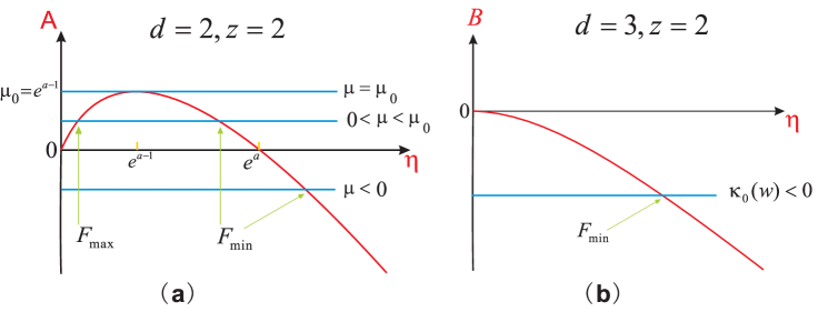
Figure S1: (a) Illustration of Eq. (S33); (b) The counterpart for the generic case of $a_{d3z2}<0$ in 3D, illustrating Eq. (S66), with $\eta=|\delta|/8.$

VI Nature of the Magnetic and Ising Transitions at Zero Temperature

We consider here the concurrent magnetic and Ising transitions at $T=0$. The RG arguments we outlined in the main text suggest that there will be a jump in the order parameters across the transitions, but the jump will be smaller as the damping parameter $\gamma$ increases. To see how damping affects the transition, we consider the parameter regime where analytical insights can be gained in our large-$N$ approach. When $\gamma$ is sufficiently large so that $x,y\ll 1$ (definitions of $x,y$ are given in the main text), it follows from the closed form of free energy [Eq. (7) in the main text] that

$$\frac{{\cal F}}{{c^{1/2}\Lambda_{c}^{3}}}=-a_{0}\left({\frac{{r(w)}}{{c\Lambda_{c}^{2}}}}\right)^{2}+\frac{{\Gamma^{3}a_{c}}}{{2\pi^{2}}}\mu(w)m_{0}^{2}+2\Gamma^{2}\left({m_{0}^{2}-\left|{\delta_{0}}\right|}\right)\sigma_{0}^{2}+\cdots$$ (S32)

where in “$\cdots$” we temporarily neglect terms at the order of $O[|\delta_{0}|^{2}\ln|\delta_{0}|]$ and $O[m_{0}^{4}\ln m_{0}^{2}]$, which will be restored when getting Eq. (S33). Also $m_{0}^{2}=m^{2}/\gamma^{2}=(x+y)/2,\;\delta_{0}=\Delta_{I}/\gamma^{2}=(x-y)/2,\;\sigma_{0}^{2}=\sigma^{2}/\left({c^{-1/2}\Lambda_{c}}\right)$. In addition $a_{c}$ and $a_{0},\;a_{,}\;\mu(w),\;\Gamma$ are respectively defined in Eq.(6) and Eq.(14) in the main text. The $a_{c}$ here is related to the ellipticity $\epsilon$ by $a_{c}=(\epsilon+1/\epsilon)/2\geq 1$; therefore, a larger $a_{c}$ means a stronger anisotropy for the system. From Eq. (S32), we see that if $r(w)$ is a large positive number, the minimum of the free energy only occurs at $\sigma_{0}=0$ and $m_{0}=0$, then $\Delta_{I}=0$, corresponding to the disordered phase of the system as expected. Eq. (S32) shows that when the system is deep inside the ordered phase with $r_{0}<0$ and $|r_{0}|\gg 1$, there is no minimum at the origin since $\mu(w)<0$. This implies that when we increase $r$ from a large negative value (deep in the ordered phase) to a certain critical point a phase transition must happen. This can be made clearer when the system stays in the ordered regime ($\sigma\neq 0$). Here in the limit $\eta\equiv|\delta_{0}|\ll 1$, to order of $(\left|{\Delta_{I}}\right|/\gamma^{2})^{2}$, we get

$$A(\eta)=a\eta-\eta\ln\eta=\mu(w)$$ (S33)

with

$$\begin{gathered}a=-\frac{{4\pi^{2}\Gamma\left({a_{I}-a_{0}}\right)}}{{a_{c}}}-\ln 2-1/2.\hfill\\ \end{gathered}$$ (S36)

We see that $a<0$ generally holds, which means the maximum of $A(\eta)$ will be $\mu_{0}=e^{a-1}$ at $\eta_{0}=e^{a-1}$. The evolution of the equation is illustrated in Fig. S1(a). When the system is in the ordered regime, i.e., $r(w)$ is a large negative number, then $\mu<0$ and there is a unique global minimum (we focus on the positive branch of the Ising order parameter). When $r(w)$ increases (via increasing $w$) to the point that $\mu=0$, there is a maximum emerging at the origin while the Ising order shrinks to $\eta_{1}=e^{a}$. After this, when $r(w)$ is further increased, the maximum emerges at the origin moves away from the origin with a cusp-type local minimum generated at the origin which can not be covered by Eqs. (S14,S33), meanwhile the Ising order shrinks further. When $r(w)$ is further increased until $\mu=\mu_{0}$, the local maximum and local minimum merge as an inflection point, and the free energy as a function of Ising order will only have a global cusp-type minimum at the origin. Therefore a first order transition happens when $e^{a-1}<\eta<e^{a}$, while tuning $w$ to $w_{c}$ such that $0<\mu(w_{c})<\mu_{0}$. From Eq. (S36) we can see larger $\Gamma$ leads to more negative $a$, since the transition happens in the regime of $e^{a-1}<\eta<e^{a}$, as a result, the first order transition would be exponentially suppressed when $\Gamma$ becomes larger, implying the transition would become essentially second order when damping becomes strong, which is consistent with RG predictions.

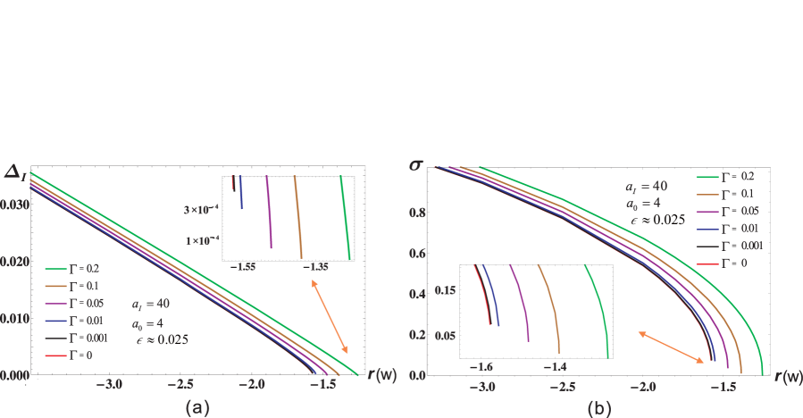
Figure S2: The evolution of Ising order (a) and antiferromagnetic order (b) as a function of the control parameter $r(w)$ at an extremely strong anisotropy $\epsilon\approx 0.025$. The jump of the order parameters becomes larger compared with the case of a moderately strong anisotropy $\epsilon\approx 0.27$ shown in Fig. 2 of the main text.

VII The Effect of Extreme Anisotropy

When the anisotropy becomes extremely large, the system effectively becomes 1D, and the effective dimensionality $d+z$ becomes 3; the quartic coupling $-u_{I}$ will become relevant (as opposed to being marginal) w.r.t. the underlying O($3$) QCP, and we expect a stronger degree of first-orderness. Indeed, as shown in Fig. S2 for an extreme value of anisotropy $\epsilon=0.025$, the magnetic order parameter jump becomes sizable.

VIII The Case of Three Spatial Dimensions

In this case, we still have the same saddle-point equation Eq. (S14), but now we take $q^{2}=q_{x}^{2}+q_{y}^{2}+q_{z}^{2}$ in ${\chi_{0,\overset{\lower 3.5pt\hbox{$\smash{\scriptscriptstyle\rightharpoonup}$}}{q},\omega_{l}}^{-1}}=r+\omega_{l}^{2}+cq^{2}+\gamma\left|{\omega_{l}}\right|$. Then at zero temperature the summation in Eq. (S14) can be calculated as follows (using Eq. (S20) and working in the regime of $\Delta_{I}=-m^{2}<0$).

$$\frac{1}{{2\beta V}}\sum\limits_{\overset{\lower 3.5pt\hbox{$\smash{\scriptscriptstyle\rightharpoonup}$}}{q},i\omega_{l}}{\frac{1}{{D_{0,\overset{\lower 3.5pt\hbox{$\smash{\scriptscriptstyle\rightharpoonup}$}}{q},i\omega_{l}}^{-1}+v\left({q_{x}^{2}-q_{y}^{2}}\right)+m^{2}-\Delta_{I}}}}=\frac{1}{{\left({2\pi}\right)^{4}}}\int_{-\Lambda_{f}}^{\Lambda_{f}}{d^{3}q\int_{0}^{\Gamma_{0}}{d\omega\frac{{\gamma\omega}}{{\left({\omega^{2}-c_{1}^{2}}\right)^{2}+\gamma^{2}\omega^{2}}}}}$$ (S37)

$$\approx \frac{1}{{8\pi^{3}}}\frac{1}{{c^{1/2}\sqrt{c^{2}-v^{2}}}}\int_{0}^{c\Lambda_{c}^{2}}{dx\frac{{i\sqrt{x}}}{{\sqrt{4x+4\left({m^{2}-\Delta_{I}}\right)-\gamma^{2}}}}\ln\frac{{\gamma-i\sqrt{4x+4\left({m^{2}-\Delta_{I}}\right)-\gamma^{2}}}}{{\gamma+i\sqrt{4x+4\left({m^{2}-\Delta_{I}}\right)-\gamma^{2}}}}}$$ (S38)

$$= \frac{1}{{64\pi^{3}}}\frac{\gamma^{2}}{{c^{1/2}\sqrt{c^{2}-v^{2}}}}\int_{0}^{\Lambda_{\gamma}}{dz\frac{{i\sqrt{z}}}{{\sqrt{z-\left({1+\delta}\right)}}}\ln\frac{{1-i\sqrt{z-\left({1+\delta}\right)}}}{{1+i\sqrt{z-\left({1+\delta}\right)}}}}$$ (S39)

$$= \frac{1}{{64\pi^{3}}}\frac{\gamma^{2}}{{c^{1/2}\sqrt{c^{2}-v^{2}}}}\left\{{\underbrace{2i\int_{\sqrt{\left|\delta\right|-1}}^{0}{dx\sqrt{x^{2}+1-\left|\delta\right|}\ln\frac{{1-ix}}{{1+ix}}}}_{I}+\underbrace{2i\int_{0}^{\sqrt{\Lambda_{\gamma}}}{dx\sqrt{x^{2}+1-\left|\delta\right|}\ln\frac{{1-ix}}{{1+ix}}}}_{II}}\right\}$$ (S40)

where $\Lambda_{\gamma}=4c\Lambda_{c}^{2}/\gamma^{2}=4/\Gamma^{2},\;\;\delta=8\Delta_{I}/\gamma^{2}$. Now let’s deal with the two integrals one by one.

$$I = 2\int_{0}^{\left({1-\left|\delta\right|}\right)^{1/2}}{dx\sqrt{1-\left|\delta\right|-x^{2}}\ln\frac{{1+x}}{{1-x}}}$$ (S41)

$$= 2\left({1-\left|\delta\right|}\right)^{1/2}\sum\limits_{n=0}^{\infty}{\frac{{(-1)^{n}}}{{\left({1-\left|\delta\right|}\right)^{n}}}\left(\begin{array}[]{l}n\\ 1/2\\ \end{array}\right)\int_{0}^{\left({1-\left|\delta\right|}\right)^{1/2}}{dxx^{2n}\ln\frac{{1+x}}{{1-x}}}}$$ (S44)

$$= 2\left({1-\left|\delta\right|}\right)^{1/2}\sum\limits_{n=0}^{\infty}{\frac{{(-1)^{n}}}{{\left({1-\left|\delta\right|}\right)^{n}}}\left(\begin{array}[]{l}n\\ 1/2\\ \end{array}\right)\left[{\frac{{\left({1-\left|\delta\right|}\right)^{n+1/2}}}{{2n+1}}\ln\frac{{1+\left({1-\left|\delta\right|}\right)^{1/2}}}{{1-\left({1-\left|\delta\right|}\right)^{1/2}}}-\int_{0}^{\left({1-\left|\delta\right|}\right)^{1/2}}{\frac{{dxx^{2n+1}}}{{2n+1}}\frac{2}{{1-x^{2}}}}}\right]}$$ (S47)

$$= 2\frac{\pi}{4}\left({1-\left|\delta\right|}\right)\ln\frac{{1+\left({1-\left|\delta\right|}\right)^{1/2}}}{{1-\left({1-\left|\delta\right|}\right)^{1/2}}}+2\left({1-\left|\delta\right|}\right)^{1/2}\sum\limits_{n=0}^{\infty}{\frac{{(-1)^{n}}}{{\left({1-\left|\delta\right|}\right)^{n}}}\left(\begin{array}[]{l}1/2\\ n\\ \end{array}\right)\left[{-\int_{0}^{\left({1-\left|\delta\right|}\right)^{1/2}}{\frac{{dxx^{2n+1}}}{{2n+1}}\frac{2}{{1-x^{2}}}}}\right]}$$ (S50)

$$= 2\frac{\pi}{4}\left({1-\left|\delta\right|}\right)\ln\frac{{1+\left({1-\left|\delta\right|}\right)^{1/2}}}{{1-\left({1-\left|\delta\right|}\right)^{1/2}}}+2\left({1-\left|\delta\right|}\right)^{1/2}\int_{0}^{\left({1-\left|\delta\right|}\right)^{1/2}}{dx\frac{{x\sqrt{1-\frac{{x^{2}}}{{1-\left|\delta\right|}}}+\sqrt{\left|\delta\right|-1}\sinh^{-1}\left({\frac{x}{{\sqrt{\left|\delta\right|-1}}}}\right)}}{{-1+x^{2}}}}$$ (S51)

$$= 2\frac{\pi}{4}\left({1-\left|\delta\right|}\right)\ln\frac{{1+\left({1-\left|\delta\right|}\right)^{1/2}}}{{1-\left({1-\left|\delta\right|}\right)^{1/2}}}+2\left[{-\left({1-\left|\delta\right|}\right)^{1/2}+\sqrt{\left|\delta\right|}\cos^{-1}\sqrt{\left|\delta\right|}}\right]$$ (S53)

$$\;\;\;\;\;\;\;\;\;\;\;\;\;\;\;\;\;\;\;\;\;\;\;\;\;\;\;\;\;\;\;\;\;\;\;\;\;\;\;\;\;\;\;\;\;\;\;\;\;\;\;\;\;+2\left({1-\left|\delta\right|}\right)^{1/2}\int_{0}^{\left({1-\left|\delta\right|}\right)^{1/2}}{dx\frac{{\sqrt{\left|\delta\right|-1}\sinh^{-1}\left({\frac{x}{{\sqrt{\left|\delta\right|-1}}}}\right)}}{{-1+x^{2}}}}$$

where $\left(\begin{array}[]{l}n\\ m\\ \end{array}\right)\equiv\frac{{\Gamma\left({n+1}\right)}}{{\Gamma\left({m+1}\right)\Gamma\left({n-m+1}\right)}}$ is the binomial coefficient. But

$$2\left({1-\left|\delta\right|}\right)^{1/2}\int_{0}^{\left({1-\left|\delta\right|}\right)^{1/2}}{dx\frac{{\sqrt{\left|\delta\right|-1}\sinh^{-1}\left({\frac{x}{{\sqrt{\left|\delta\right|-1}}}}\right)}}{{-1+x^{2}}}}$$ (S54)

$$= 2\left({1-\left|\delta\right|}\right)^{1/2}\left\{{\left.{\sqrt{\left|\delta\right|-1}\left({-\tanh^{-1}x}\right)\sinh^{-1}\left({\frac{x}{{\sqrt{\left|\delta\right|-1}}}}\right)}\right|_{x=0}^{\left({1-\left|\delta\right|}\right)^{1/2}}+\int_{0}^{\left({1-\left|\delta\right|}\right)^{1/2}}{dx\frac{{\tanh^{-1}x}}{{\sqrt{1-x^{2}/(1-\left|\delta\right|)}}}}}\right\}$$ (S56)

$$= -2\frac{\pi}{4}\left({1-\left|\delta\right|}\right)\ln\frac{{1+\left({1-\left|\delta\right|}\right)^{1/2}}}{{1-\left({1-\left|\delta\right|}\right)^{1/2}}}+2\left({1-\left|\delta\right|}\right)^{1/2}\frac{i}{4}\left({1-\left|\delta\right|}\right)^{1/2}\left\{{\pi^{2}-4\cosh^{-1}\sqrt{\left|\delta\right|}\ln\left({-i\left({1-\sqrt{\left|\delta\right|}}\right)/\sqrt{1-\left|\delta\right|}}\right)}\right.$$

$$\;\;\;\;\;\;\;\;\;\;\;\;\;\;\;\;\;\;\;\;\;\;\;\;\;\;\;\;\;\;\;\;\;\;\;\;\;\;\;\;\;\;\;\;\;\;\;\;\;\;\;\;\;\;\;\left.{+4{\text{Li}}_{2}\left({-i\left({1-\left|\delta\right|}\right)^{1/2}-\sqrt{\left|\delta\right|}}\right)-4{\text{Li}}_{2}\left({i\left({1-\left|\delta\right|}\right)^{1/2}+\sqrt{\left|\delta\right|}}\right)}\right\}$$

where ${\text{Li}}_{n}(z)=\sum\limits_{k=1}^{\infty}{\frac{{z^{k}}}{{k^{n}}}}$ is the polylogarithm function. Substituting Eq. (S56) back into Eq. (S53), we have

$$I=2\left[{-\left({1-\left|\delta\right|}\right)^{1/2}+\sqrt{\left|\delta\right|}\cos^{-1}\sqrt{\left|\delta\right|}}\right]+\frac{i}{{\text{2}}}\left({1-\left|\delta\right|}\right)\left\{{\pi^{2}-4\cosh^{-1}\sqrt{\left|\delta\right|}\ln\left({-i\left({1-\sqrt{\left|\delta\right|}}\right)/\sqrt{1-\left|\delta\right|}}\right)}\right.$$

$$\;\;\;\;\;\;\;\;\;\;\;\;\;\;\;\;\;\;\;\;\;\;\;\;\;\;\;\;\;\;\;\;\;\;\;\;\;\;\;\;\;\;\;\;\;\;\;\;\;\;\left.{+4{\text{Li}}_{2}\left({-i\left({1-\left|\delta\right|}\right)^{1/2}-\sqrt{\left|\delta\right|}}\right)-4{\text{Li}}_{2}\left({i\left({1-\left|\delta\right|}\right)^{1/2}+\sqrt{\left|\delta\right|}}\right)}\right\}$$ (S57)

Note Eq. (S56) is an exact result for the integral $I$ in Eq. (S40). For simplicity here we only consider the analytic limit at $|\delta|=8|\Delta_{I}|/\gamma^{2}\ll 1$. Within this limit we can get an expansion series of Eq. (S57) in the order of $|\delta|$,

$$I=2\left\{{-1+2\alpha_{0}-2\alpha_{0}\left|\delta\right|+\frac{\pi}{3}\left|\delta\right|^{3/2}-\frac{1}{4}\left|\delta\right|^{2}+O\left({\left|\delta\right|^{5/2}}\right)}\right\}$$ (S58)

where $\alpha_{0}\approx 0.91596$ is the Catalan number.

Now we calculate the integral $II$ in Eq. (S40), which is straightforward in the limit of $|\delta|=8|\Delta_{I}|/\gamma^{2}\ll 1$.

$$II=2i\int_{0}^{\sqrt{\Lambda_{\gamma}}}{dx\sqrt{x^{2}+1-\left|\delta\right|}\ln\frac{{1-ix}}{{1+ix}}}=4\int_{0}^{\sqrt{\Lambda_{\gamma}}}{dx\sqrt{x^{2}+1}\tan^{-1}x}-2\left|\delta\right|\int_{0}^{\sqrt{\Lambda_{\gamma}}}{dx\frac{{\tan^{-1}x}}{{\sqrt{1+x^{2}}}}}+O\left({\left|\delta\right|^{2}}\right)$$ (S59)

but

$$4\int_{0}^{\sqrt{\Lambda_{\gamma}}}{dx\sqrt{x^{2}+1}\tan^{-1}x}$$ (S60)

$$= 4\left\{{\frac{1}{2}\left.{\left[{\sqrt{1+x^{2}}\left({x\tan^{-1}x-1}\right)+\tan^{-1}x\ln\frac{{1-ie^{i\tan^{-1}x}}}{{1+ie^{i\tan^{-1}x}}}+i{\text{Li}}_{2}\left({-ie^{i\tan^{-1}x}}\right)-i{\text{Li}}_{2}\left({ie^{i\tan^{-1}x}}\right)}\right]}\right|_{x=0}^{\sqrt{\Lambda_{\gamma}}}}\right\}$$

$$= \pi\Lambda_{\gamma}-4\sqrt{\Lambda_{\gamma}}+\frac{\pi}{2}\ln\Lambda_{\gamma}+\frac{\pi}{2}\left({1+2\ln 2}\right)+2-4\alpha_{0}+O\left({\frac{1}{{\sqrt{\Lambda_{\gamma}}}}}\right)$$

and

$$\int_{0}^{\sqrt{\Lambda_{\gamma}}}{dx\frac{{\tan^{-1}x}}{{\sqrt{x^{2}+1}}}}=\left.{\left[{\tan^{-1}x\ln\frac{{1-ie^{i\tan^{-1}x}}}{{1+ie^{i\tan^{-1}x}}}+i{\text{Li}}_{2}\left({-ie^{i\tan^{-1}x}}\right)-i{\text{Li}}_{2}\left({ie^{i\tan^{-1}x}}\right)}\right]}\right|_{x=0}^{\sqrt{\Lambda_{\gamma}}}$$ (S61)

$$= \frac{\pi}{2}\ln 2-2\alpha_{0}+\frac{\pi}{4}\ln\Lambda_{\gamma}+O\left({\frac{1}{{\sqrt{\Lambda_{\gamma}}}}}\right)$$

Substituting the results of Eqs. (S60,S61) into Eq. (S59), we have

$$II=\pi\Lambda_{\gamma}-4\sqrt{\Lambda_{\gamma}}+\frac{\pi}{2}\ln\Lambda_{\gamma}+\frac{\pi}{2}\left({1+2\ln 2}\right)+2-4\alpha_{0}-2\left|\delta\right|\left({\frac{\pi}{2}\ln 2-2\alpha_{0}+\frac{\pi}{4}\ln\Lambda_{\gamma}}\right)+O\left({\frac{1}{{\sqrt{\Lambda_{\gamma}}}}}\right)+O(|\delta|^{2})$$ (S62)

Combining the results in Eqs. (S58,S62), we finally have

$$I+II=\pi\Lambda_{\gamma}-4\sqrt{\Lambda_{\gamma}}+\frac{\pi}{2}\ln\Lambda_{\gamma}+\frac{\pi}{2}\left({1+2\ln 2}\right)-\left({\pi\ln 2+\frac{\pi}{2}\ln\Lambda_{\gamma}}\right)\left|\delta\right|+\frac{\pi}{3}\left|\delta\right|^{3/2}+O\left({\frac{1}{{\sqrt{\Lambda_{\gamma}}}}}\right)+O(|\delta|^{2})$$ (S63)

Substituting Eq. (S63) into Eq. (S14), we have

$$\frac{{\alpha_{c}\Delta_{I}}}{{u_{I}\gamma^{2}}}=\frac{{\alpha_{c}\Delta_{I}}}{{(2u_{1}+u_{2})\gamma^{2}}}+\kappa_{\text{0}}-\kappa_{\text{1}}\left|\delta\right|+\frac{{\pi}}{3}|\delta|^{3/2}+O(\delta^{2})$$ (S64)

with $\alpha_{c}=64\pi^{3}c^{1/2}\sqrt{c^{2}-v^{2}}$, and

$$\kappa_{\text{0}}(w)=\frac{\alpha_{c}r(w)}{{(2u_{1}+u_{2})\gamma^{2}}}+\pi\Lambda_{\gamma}-4\sqrt{\Lambda_{\gamma}}+\frac{\pi}{2}\ln\Lambda_{\gamma}+\frac{\pi}{2}\left({1+2\ln 2}\right);\kappa_{1}=\pi\ln 2+\frac{\pi}{2}\ln\Lambda_{\gamma}=\pi\ln 2+\frac{\pi}{2}\ln\frac{4}{\Gamma^{2}}$$ (S65)

Then we have

$$B(|\delta|)\equiv a_{d3z2}\left|\delta\right|-\frac{{2\pi}}{3}\left|\delta\right|^{3/2}=\kappa_{\text{0}}(w)$$ (S66)

with

$$a_{d3z2}=-\frac{{\alpha_{c}}}{4}\left({\frac{1}{{u_{I}}}-\frac{1}{{2u_{1}+u_{2}}}}\right)+2\kappa_{1}=-\frac{{16\pi^{3}}}{{a_{c}}}\left({\frac{{c^{3/2}}}{{u_{I}}}-\frac{{c^{3/2}}}{{2u_{1}+u_{2}}}}\right)+2\kappa_{1}$$ (S67)

From Eq. (S66) we can see that the sign of $a_{d3z2}$ will determine the order(s) of the phase transition. If $a_{d3z2}<0$, there is no first order transition since Eq. (S66) always has only one solution; the Ising order parameter will continuously go to zero as we increase the controlled parameter $w$ in $\kappa_{0}(w)$. Fig. S1(b) illustrates the process for the phase transitions at $a_{d3z2}<0$.

If $a_{d3z2}>0$, a first order transition can happen, since two solutions of Eq. (S66) emerge when $\kappa_{0}(w)>0$. From the LHS of Eq. (S66), we can determine that $a_{d3z2}>0$ can happen either at $v\approx c$ (i.e., extreme anisotropy) or at extremely small damping rate. In the former case the system is effectively reduced back to the 3D problem, where we roughly recover the 2D results. For the latter case, it is equivalent to changing the effective dimension $d+z=d+2$ to $d+1$. Therefore in both of these two extreme situations, the effective dimension of the system becomes 4; the Ising coupling “$-u_{I}$” is again marginal, and a first-order transition is to be expected from RG-based considerations. For the problem we are considering, neither case applies.

For the summation in Eq. (S13), a similar calculation can be carried out. One can easily find that it is $\delta$-independent, which is just equal to the $\delta$-independent part of the summation in Eq. (S14). Therefore after summing Eq. (S13) and Eq. (S14) we will get,

$$\frac{{2\Delta_{I}}}{{u_{I}}}=-2\sigma^{2}+\frac{{\gamma^{2}}}{{\alpha_{c}}}\left({-\kappa_{1}\left|\delta\right|+\frac{\pi}{3}\left|\delta\right|^{3/2}+O\left({\frac{1}{{\sqrt{\Lambda_{\gamma}}}}}\right)+O\left({\left|\delta\right|^{2}}\right)}\right)$$ (S68)

i.e.,

$$\sigma_{0}=\frac{\Gamma}{{8\pi}}\sqrt{\frac{{a_{c}}}{\pi}}\sqrt{\frac{1}{2}\left({\frac{{16\pi^{3}}}{{a_{c}}}\frac{{c^{3/2}}}{{u_{I}}}-\kappa_{1}}\right)\left|\delta\right|+\frac{\pi}{6}\left|\delta\right|^{3/2}}$$ (S69)

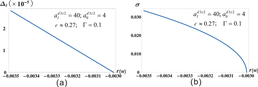
Figure S3: Evolution of (a) the Ising order parameter and (b) the magnetic order parameter vs. the control parameter at a moderate strong anisotropy, for the 3D case.

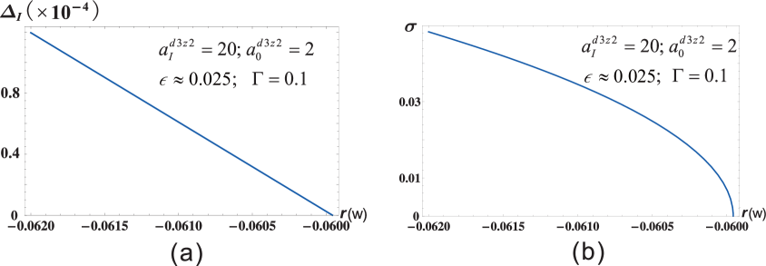
Figure S4: Evolution of (a) the Ising order parameter and (b) the magnetic order parameter vs. the control parameter at an extremely strong anisotropy, and with strong interactions, also in the 3D case.

with dimensionless magnetization $\sigma_{0}=c^{1/4}\sigma/\Lambda_{c}$. From Eq. (S69) we can see that when $\delta$ continues to zero, the magnetization will also continuously go to zero, indicating a second-order magnetic phase transition, and the concurrence of Ising and magnetic phase transitions. From Eqs. (S66,S69), we can get Ising order and magnetic order vs. the control parameter $r(w)$ in $d=3,\,z=2$ systems in the limit of $|\delta|=8|\Delta_{I}|/\gamma^{2}\ll 1$, as shown in Figs. (S3,S4), where the Ising order $\Delta_{I}$ and magnetic order $\sigma$ have been respectively re-scaled into dimensionless quantities via $\Delta_{I}\to\Delta_{I}/(c\Lambda_{c}^{2})$ and $\sigma\to c^{1/4}\sigma/\Lambda_{c}=\sigma_{0}$ (for convenience we also introduce a group of dimensionless parameters $a_{I}^{d3z2}=c^{3/2}/u_{I},a_{0}^{d3z2}=c^{3/2}/(2u_{1}+u_{2}),a_{c}=c/\sqrt{c^{2}-v^{2}},\Gamma=\gamma/(c^{1/2}\Lambda_{c})$). At moderate strong anisotropy $\epsilon\approx 0.27$ (Fig. S3), it shows continuous quantum phase transitions and concurrence of the Ising and magnetic orders when increasing $w$. As in the 2D case we also study the effect of strong anisotropy at $\epsilon\approx 0.025$ (Fig. S4), where the continuous phase transitions persist, and the two transitions are concurrent. This is consistent with the RG considerations: given that the effective dimensionality in this case is $d+z=5$, the quartic coupling $-u_{I}$ becomes irrelevant w.r.t. to the underlying O($3$) transition and will therefore not destabilize the continuous nature of the transition.

References

- (1) Y. Kamihara, T. Watanabe, M. Hirano, and H. Hosono, J. Am. Chem. Soc. 130, 3296 (2008).
- (2) C. de la Cruz et al., Nature 453, 899 (2008).
- (3) J. Dai, Q. Si, J-X Zhu, and E. Abrahams, PNAS 106, 4118 (2009).
- (4) M. Qazilbash et al., Nature Phys. 5, 647 (2009).
- (5) W. Z. Hu et al., Phys. Rev. Lett. 101, 257005 (2008).
- (6) L. Degiorgi, New J. Phys. 13, 023011 (2011).
- (7) M. Nakajima et al., Sci. Rep. 4, 5873 (2014).
- (8) Q. Si and E. Abrahams, Phys. Rev. Lett. 101, 076401 (2008).
- (9) Q. Si, E. Abrahams, J. Dai and J.-X. Zhu, New J. Phys. 11, 045001 (2009).
- (10) Z. P. Yin, K. Haule, and G. Kotliar, Nat. Mat. 10, 932 (2011).
- (11) P. Quebe, L. J. Terbuchte, and W. Jeitschko, J. Alloys Compd. 302, 70 (2000).
- (12) B. I. Zimmer, J. Alloys Compd. 229, 238 (1995).
- (13) E. Abrahams and Q. Si, J. Phys.: Condens. Matter 23, 223201 (2011).
- (14) C. de la Cruz, et al., Phys Rev Lett 104, 017204 (2010).
- (15) Y. Luo, et al., Phys. Rev. B 81, 134422 (2010).
- (16) S. Kasahara, et al., Phys Rev B 81, 184519 (2010).
- (17) Y. Nakai, et al., Phys. Rev. Lett. 105, 107003(2010).
- (18) K. Hashimoto et al, Science 336, 1554 (2012).
- (19) J. G. Analytis et al, Nature Phys. 10, 194 (2014).
- (20) I. M. Hayes et al, arXiv:1412.6484.
- (21) S. Kasahara et al., Nature 486, 382 (2012).
- (22) P. Chandra, P. Coleman, and A. I. Larkin, Phys. Rev. Lett. 64, 88 (1990).
- (23) C. Fang, H. Yao, W. F. Tsai, J. P. Hu, and S. A. Kivelson, Phys. Rev. B 77, 224509 (2008).
- (24) C. Xu, M. Müller and S. Sachdev, Phys. Rev. B78, 020501 (2008).
- (25) R. M. Fernandes et al., Phys. Rev. Lett 111, 057001 (2013); Phys. Rev. B85, 024534 (2012).
- (26) A. Rançon, O. Kodio, N. Dupuis, and P. Lecheminant, Phys. Rev. E 88, 012113 (2013).
- (27) S. Coleman, R. Jackiw, and H. D. Politzer, Phys. Rev. D 10, 2491 (1974).
- (28) D. Hu et al., Phys. Rev. lett. 114, 157002 (2015).
- (29) G. Moeller, Q. Si, G. Kotliar, M. Rozenberg, and D. S. Fisher, Phys. Rev. Lett. 74, 2082 (1995).
- (30) T. Yildirim, Phys. Rev. Lett. 101, 057010 (2008).
- (31) F. Ma, Z-Y Lu, and T. Xiang, Phys. Rev. B 78, 224517 (2008).
- (32) C. L. Henley, Phys. Rev. Lett. 62, 2056 (1989).
- (33) R.Yu, Z. Wang, P. Goswami, A. H. Nevidomskyy, Q. Si, and E. Abrahams, Phys. Rev. B86, 085148 (2012).
- (34) A. L. Wysocki, K. D. Belashchenko and V. P. Antropov, Nat. Phys. 7, 485 (2011).
- (35) Y. Qi and C. Xu, Phys. Rev. B 80, 094402 (2009).
- (36) P. Goswami, R. Yu, Q. Si, and E. Abrahams, Phys. Rev. B 84, 155108 (2011).
- (37) See Supplemental Material, which includes Ref. Negele1998 , for details of derivations and solutions of the variational equations.
- (38) J. Negele and H. Orland, Quantum Many-Particle Systems, Westview Press, (1998).
- (39) S. O. Diallo et al. Phys. Rev. B 81, 214407 (2010).
- (40) H. Shishido et al., Phys. Rev. Lett. 104, 057008 (2010).
- (41) X. Lu et al., Science 345, 657 (2014).
- (42) Y. Song et al., Phys. Rev. B92, 180504(R) (2015).
- (43) L. W. Harriger et al., Phys. Rev. B 84, 054544 (2011).
- (44) R. Yu et al., Nat. Commun. 4, 2783 (2013).
- (45) J. Guo et al., Phys. Rev. B 82, 180520 (2010).
- (46) M.-H. Fang et al., Europhys. Lett. 94, 27009 (2011).
- (47) Q.-Y. Wang et al., Chin. Phys. Lett. 29, 037402 (2012).
- (48) S. He et al., Nat. Mater. 12, 605 (2013).
- (49) J. J. Lee et al., Nature 515, 245 (2014).
- (50) Z. Zhang et al., Science Bulletin 60, 1301 (2015).