Abstract

The entanglement entropy for interfaces and junctions of two-dimensional CFTs is evaluated on holographically dual half-BPS solutions to six-dimensional Type 4b supergravity with $m$ anti-symmetric tensor supermultiplets. It is shown that the moduli space for an $N$-junction solution projects to $N$ points in the Kähler manifold $SO(2,m)/\left(SO(2)\times SO(m)\right)$. For $N=2$ the interface entropy is expressed in terms of the central charge and Calabi’s diastasis function on $SO(2,m)/\left(SO(2)\times SO(m)\right)$, thereby lending support from holography to a proposal of Bachas, Brunner, Douglas, and Rastelli. For $N=3$, the entanglement entropy for a 3-junction decomposes into a sum of diastasis functions between pairs, weighed by combinations of the three central charges, provided the flux charges are all parallel to one another or, more generally, provided the space of flux charges is orthogonal to the space of unattracted scalars. Under similar assumptions for $N\geq 4$, the entanglement entropy for the $N$-junction solves a variational problem whose data consist of the $N$ central charges, and the diastasis function evaluated between pairs of $N$ asymptotic $AdS_{3}\times S^{3}$ regions.

1 Introduction

An increasingly compelling connection has been emerging between entropy and geometry ever since Bekenstein and Hawking assigned an entropy to a quantum black hole. Gauge/gravity duality [1, 2, 3] relates the entropy of a thermal state in quantum field theory to the entropy of a black holes in the gravity dual. The Ryu-Takayanagi proposal [4, 5] gives a holographic formula for the entanglement entropy in conformal field theory associated with a spatial region ${\cal A}$ in terms of the area of a minimal surface in the bulk gravity theory subtended by the region ${\cal A}$. For conformal field theories with interfaces or boundaries, the entanglement entropy provides information on the degeneracy of the ground state $\mathfrak{g}$-function, also referred to as the interface or boundary entropy [6].

Superconformal gauge theories in which an interface, a defect, or a boundary is preserved by part of the superconformal symmetry have been the subject of intense study, in large part because these theories often provide solvable yet non-trivial deformations of the original theory. Such studies include probe brane constructions [7]; the construction of two-dimensional conformal interfaces by the folding trick [8]; the discovery of topological defects and their algebra [9, 10]; the analysis of supersymmetry preserving interfaces in four-dimensional ${\cal N}=4$ super-Yang-Mills [11, 12, 13, 14]; and the interplay between defect and domain wall operators [15, 16]. Rich families of supersymmetric fully back-reacted solutions have been constructed in Type IIB supergravity for supersymmetric interfaces in [18, 19] and Wilson lines in [20, 21]; in M-theory for defects in [22, 23, 24]; and in various supergravities for junctions of CFTs in two dimensions in [25, 26, 27, 28].

A intriguing novel connection was proposed in [29] between the interface entropy in certain two-dimensional CFTs and Calabi’s diastasis function of Kähler geometry. In string theory, Kähler geometry governs compactifications which preserve various degrees of space-time supersymmetry. The moduli spaces of the corresponding $(2,2)$ supersymmetric sigma models generically have Kähler moduli and complex structure moduli components.

The Calabi diastasis function [30] may be defined for any Kähler manifold ${\cal K}$ with Kähler form $\omega=i\partial\bar{\partial}K$ and associated Kähler potential $K$. The Kähler form $\omega$ is invariant under Kähler gauge transformations, which may be expressed in local complex coordinates $(t,\bar{t})$ by $K(t,\bar{t})\to K(t,\bar{t})+\Lambda(t)+\bar{\Lambda}(\bar{t})$, where $\Lambda(t)$ is holomorphic. Calabi showed [30] that the real-valued Kähler potential $K(t,\bar{t})$ may be continued to a complex-valued potential $K(t_{1},\bar{t}_{2})$ for independent points $t_{1}$ and $t_{2}$. The diastasis function,

$${\cal D}(1,2)=K(t_{1},\bar{t}_{1})+K(t_{2},\bar{t}_{2})-K(t_{1},\bar{t}_{2})-K(t_{2},\bar{t}_{1})$$ (1.1)

is then well-defined, invariant under Kähler gauge transformations, and preserved upon restriction to a complex analytic submanifold of ${\cal K}$. In the limit where the points $t_{1},t_{2}$ are infinitesimally near one another, ${\cal D}(1,2)$ reduces to the Kähler metric on ${\cal K}$.

Specifically, a formula was proposed in [29] for the $\mathfrak{g}$-function of an interface separating $(2,2)$ supersymmetric CFTs with Kähler moduli $t_{1}$ and $t_{2}$ in terms of the diastasis function,

$$2\ln\mathfrak{g}={\cal D}(1,2)$$ (1.2)

In turn, the $\mathfrak{g}$-function is related to the entanglement entropy of a spatial region of length $L$ which encloses the interface symmetrically, by the following relation [34],

$$S_{\varepsilon}={c\over 3}\ln{L\over\varepsilon}+\ln\mathfrak{g}$$ (1.3)

The examples given in [29] to illustrate the relation (1.2) include sigma models with $(2,2)$ supersymmetry, for target space $T^{2}$ as well as Calabi-Yau manifolds in the large volume limit. A common feature of these examples is the fact that (1.2) holds only for a special subclass of interfaces which preserve some supersymmetry, and for interfaces where the moduli of either the complex structure or the Kähler structure are held fixed across the interface.

1.1 Summary of results

In the present paper we shall produce evidence supporting the relation (1.2) between the interface entropy and Calabi’s diastasis function using the holographically dual half-BPS interface solutions [27] to Type 4b supergravity [31]. The fundamental property of these families of solutions that makes this correspondence possible is the existence of a smooth projection from their $(3m+2)$-dimensional moduli space to a pair of points in the Kähler manifold $SO(2,m)/\left(SO(2)\times SO(m)\right)$. The points correspond to the two asymptotic $AdS_{3}\times S^{3}$ regions of the interface, and are subject to the overall conservation of anti-symmetric tensor field flux charge. The interface entropy is then determined by the Calabi diastasis function evaluated at this pair of points, along with the common central charge of these regions. Essential in making this connection is the fact that the holographic interface solution preserves some supersymmetry. Note that supersymmetry was also a crucial ingredient on the CFT side, as discussed in [29]. There is was shown that the relation of $\mathfrak{g}$-function and diastasis function does not hold for a non-supersymmetric interface where both the Kähler and complex moduli jump. A holographic example of this failure is given in section 8, where it is shown that for a nonsupersymmetric Janus interface the $\mathfrak{g}$-function is related to the geodesic distance between points in the moduli space rather than to the diastasis function.

Next, we shall define and evaluate the entanglement entropy of the half-BPS solutions to Type 4b supergravity which are dual to $N$-junctions. The corresponding $N$-junctions solutions were obtained explicitly in [27]. Their space-time manifold is of the form $AdS_{2}\times S^{2}$ warped over a Riemann surface $\Sigma$ with boundary $\partial\Sigma$. The solutions have $N$ asymptotic $AdS_{3}\times S^{3}$ regions labelled by $i=1,\cdots,N$, each of which is characterized by a unit vector $\hat{\kappa}_{i}\in{\mathbb{R}}^{m+2}$ of vacuum expectation values of the un-attracted scalars, as well as a charge vector $\mu_{i}\in{\mathbb{R}}^{m+2}$ which obeys $\mu_{i}\cdot\mu_{i}>0$, overall charge conservation $\sum_{i=1}^{N}\mu_{i}=0$, as well as $\mu_{i}\cdot\hat{\kappa}_{i}=0$. The data $\hat{\kappa}_{i},\mu_{i}$, subject to the above relations, account for the $2(m+1)N-m-2$ moduli of these families of solutions, including for the central charge $c_{i}\sim\mu_{i}\cdot\mu_{i}$ of each asymptotic region.

The supergravity fields of the general half-BPS $N$-junction solutions are completely determined in terms of $\hat{\kappa}_{i}$ and $\mu_{i}$ by the BPS equations and Bianchi identities [27]. We shall prove a key result that all data are equivalently and uniquely determined by extremizing the holographic entanglement entropy for given $\hat{\kappa}_{i}$ and $\mu_{i}$. This result may be interpreted as a realization (albeit in a “mini-superspace” sense) of the idea that gravitational equations of motion follow from entanglement entropy (see e.g. [32, 33])

Finally, we shall derive generalizations applicable to the entanglement entropy of the junctions of $N\geq 3$ CFTs, each of which lives on a spatial half-line, and which are joined at a single spatial point. We shall often refer to the entanglement entropy in this case as junction entropy, and derive a general formula for the junction entropy of all such solutions in terms of the data $\hat{\kappa}_{i}$ and $\mu_{i}$ for $i=1,\cdots,N$. For special arrangements of the charges, such as when all charge vectors being parallel to one another, we shall express the junction entropy as a sum of terms each of which is governed by the diastasis function for a pair of $AdS_{3}\times S^{3}$ regions. We end by speculating on the significance of the junction entropy as an $N$-point generalization of the diastasis function with $N\geq 3$. We shall also briefly discuss the possible significance of the special arrangements of charges upon which the junction entropy reduces to a dependence on Calabi’s diastasis function only.

1.2 Organization

The remainder of this paper is organized as follows. In section 2 we review the six-dimensional Type 4b supergravity solutions which are half-BPS and describe holographic interfaces and junctions. In section 3 we calculate the entanglement entropy for the general $N$-junction solution. In section 4 we analyze the Kähler structure of the moduli space of half-BPS solutions and express the diastasis function in terms of the supergravity fields. In section 5 we give a holographic proof of the relation (1.2) between the interface entropy and the diastasis function for $N=2$. In section 6 we calculate the entanglement entropy of the holographic solutions which are dual to junctions of three CFTs. Specializing to the case of parallel charges $\mu_{i}$, or when $\hat{\kappa}_{i}\cdot\mu_{j}=0$ for all $i,j$, we express the junction entropy as a sum of diastasis functions of pairs of asymptotic data. In section 7 we present an analogous treatment for the case of $N$-junctions. We close in section 8 with a calculation of the entropy for a non-supersymmetric interface, and in section 9 with a discussion of our results and future directions. Some review material and technical details of the UV regularization of the holographic entropy are relegated to Appendix A.

2 Holographic Interfaces and Junctions

The holographic dual to two-dimensional CFTs with an interface or a junction will be formulated in terms of six-dimensional Type 4b supergravity [31], a family of theories which contain a supergravity supermultiplet and $m$ anti-symmetric tensor supermultiplets. The bosonic fields consist of the metric, two-form fields of which 5 have self-dual and $m$ have anti-self dual field strength, and $5m$ scalars in the $SO(5,m)/\left(SO(5)\times SO(m)\right)$ coset. The fermionic fields consist of four negative chirality gravitinos and $4m$ positive chirality spinors. Classically, the number $m$ is arbitrary and the supergravity Bianchi identities and field equations are invariant under $SO(5,m,{\mathbb{R}})$. At the quantum level, however, the absence of anomalies requires $m=5$ or $m=21$, and restricts invariance to the U-duality group $SO(5,m,{\mathbb{Z}})$. The theory corresponds to the low energy limit of Type IIB string theory compactified respectively on the spaces $T^{4}$ or $K3$.

The vacuum solution has space-time $AdS_{3}\times S^{3}$ and is invariant under the isometry $PSU(1,1|2)\times PSU(1,1|2)$ Lie superalgebra. The dual CFT has a central charge related to the radius of $AdS_{3}$ by the Brown-Henneaux formula [35].

A half-BPS solution which is holographically dual to the interface of two CFTs interpolates between two asymptotic $AdS_{3}\times S^{3}$ regions with the same central charge. A half-BPS solution dual to the junction of $N$ different CFTs is characterized by a space-time with $N$ asymptotic $AdS_{3}\times S^{3}$ regions, in which the radii of the asymptotic $AdS_{3}$ are subject to certain mild inequalities. Regular solutions to Type 4b supergravity with these properties exist for arbitrary $m$ and have been constructed explicitly in [27, 36].

2.1 Half-BPS supergravity solutions in Type 4b

In this section we shall briefly review the salient features of the half-BPS solutions to Type 4b supergravity of [27, 36] which are dual to interface and junction CFTs. The structure of their space-time manifold is dictated by supersymmetry. It takes the form of $AdS_{2}\times S^{2}$ warped over a Riemann surface $\Sigma$ with boundary and enjoys a $SO(2,1)\times SO(3)$ isometry.

The space-time metric $ds^{2}$ of the solutions and its closed 3-form field strengths $G^{A}$ with $A=1,\cdots,m+5$, are given as follows,

$$ds^{2} = H{F_{+}\over F_{-}}\,ds_{AdS_{2}}^{2}+H{F_{-}\over F_{+}}\,ds^{2}_{S^{2}}+{F_{+}F_{-}\over H}|dw|^{2}$$

$$G^{A} = d\Psi^{A}\wedge\omega_{AdS_{2}}+d\Phi^{A}\wedge\omega_{S^{2}}$$ (2.1)

Here, $w,\bar{w}$ are local complex coordinates on $\Sigma$, while $ds^{2}_{AdS_{2}}$ and $ds^{2}_{S^{2}}$ are the metrics respectively of the manifolds $AdS_{2}$ and $S^{2}$ with unit radius, and $\omega_{AdS_{2}}$ and $\omega_{S^{2}}$ are their respective volume forms. The remaining data, namely $H$, $F_{\pm}$, $\Phi^{A}$ and $\Psi^{A}$ are all real-valued functions on $\Sigma$, which we shall now specify.

The BPS equations and regularity conditions require $H$ to be a positive harmonic function in the interior of $\Sigma$ which vanishes on the boundary $\partial\Sigma$ of $\Sigma$. They also require $F_{\pm}^{2}$ to be positive in the interior of $\Sigma$ and $F_{-}$ to vanish on $\partial\Sigma$. The BPS equations, along with the Bianchi identities, then determine the remaining data in terms of an $SO(5,m)$-vector $\Lambda$ of meromorphic functions on $\Sigma$ satisfying,

$$0 = \Lambda\cdot\Lambda-2(\partial_{w}H)^{2}$$

$$F_{\pm}^{2} = \bar{\Lambda}\cdot\Lambda\pm 2|\partial_{w}H|^{2}$$ (2.2)

The dot product is taken with respect to the $SO(5,m)$-invariant metric $\eta=\hbox{diag}(I_{5},-I_{m})$. The real-valued flux potentials $\Phi^{A}$ and $\Psi^{A}$ are given in terms of the complex combination,

$${1\over\sqrt{2}}\left(\Phi^{A}-i\Psi^{A}\right)={H\partial_{w}H\over F_{+}^{2}F_{-}^{2}}\Big{(}(\bar{\Lambda}\cdot\bar{\Lambda})\,\Lambda^{A}-(\bar{\Lambda}\cdot\Lambda)\,\bar{\Lambda}^{A}\Big{)}-\int dw\,\Lambda^{A}$$ (2.3)

It is a fundamental result, obtained in [27], that the BPS equations require invariance of half-BPS solutions under an $SO(3)$ subgroup of the $SO(5)$ factor of $SO(5)\times SO(m)$. The $SO(3)$ is minimal in $SO(5)$ so that the vector of $SO(5)$ decomposes under $SO(3)$ as follows ${\bf 5}={\bf 3}\oplus{\bf 1}\oplus{\bf 1}$. As a result, the invariance of any $SO(5,m)$ vector under this $SO(3)$ requires the vanishing of the corresponding components of the vector. We shall choose a gauge in which $G^{A}=\Phi^{A}=\Psi^{A}=\Lambda^{A}=0$ for $A=3,4,5$.

Finally, the matrix of scalar fields $V$ takes values in $SO(5,m)/\left(SO(5)\times SO(m)\right)$, so that we have $V^{t}\eta V=\eta$, where $\eta=\hbox{diag}(I_{5},-I_{m})$. We shall denote its components by $V=V^{(\rho,r)}{}_{A}$ with $\rho=1,\cdots,5$ and $r=6,\cdots,m+5$. The $SO(3)$ invariance of the solutions implies that we should set $V^{(\rho,r)}{}_{A}=\delta^{\rho}{}_{A}$ for $A=3,4,5$ as well as for $\rho=3,4,5$. The remaining $V$ effectively takes values in the reduced space $SO(2,m)/\left(SO(2)\times SO(m)\right)$, and may be parametrized, uniquely up to rotations in $SO(2)\times SO(m)$, by the entries,

$$V^{\pm}{}_{A}={1\over\sqrt{2}}\left(V^{1}{}_{A}\pm iV^{2}{}_{A}\right)\hskip 72.26999ptV^{+}{}_{A}=\left(\bar{\lambda}_{A}-|X|^{2}\lambda_{A}\right)\,X\,(1-|X|^{4})^{-1}$$ (2.4)

with $|X|^{2}+|X|^{-2}=\bar{\Lambda}\cdot\Lambda/|\partial_{w}H|^{2}$. In particular, the phase of the function $X$ remains undetermined, as it transforms non-trivially under $SO(2)$ rotations in $SO(2)\times SO(m)$.

Note that the effective target space $SO(2,m)/\left(SO(2)\times SO(m)\right)$ of the scalar fields is the Kähler manifold which will govern the Calabi diastasis structure to be established below.

2.2 Parametrization of the supergravity solutions

We limit attention here to the case where the Riemann surface $\Sigma$ has only a single connected boundary component and no handles, so that it may be modeled by the upper half plane. Positivity of $H$ and $F_{\pm}^{2}$ in the interior of $\Sigma$ forces all poles $x_{i}$ of the harmonic function $H$ to lie on the real line, and $\Lambda$ to have single and double poles at $x_{i}$. Regularity of the solution precludes $\Lambda$ from having singularities away from the points $x_{i}$.

Near each pole $x_{i}$ the metric becomes locally asymptotic to $AdS_{3}\times S^{3}$ and corresponds to a half-line CFT holographic dual. Thus a supergravity solution with $N$ poles $x_{i}$ for $i=1,\cdots,N$ will produce a holographic dual consisting of a junction of $N$ half-line CFTs. The basic functions of these solution take the following form,

$$H = i\sum_{i=1}^{N}\left({\gamma_{i}\over w-x_{i}}-{\gamma_{i}\over\bar{w}-x_{i}}\right)$$

$$\Lambda^{A} = -i\sum_{i=1}^{N}\left({\kappa_{i}^{A}\over(w-x_{i})^{2}}+{\mu_{i}^{A}\over w-x_{i}}\right)$$ (2.5)

The residues $\gamma_{i},\kappa_{i}^{A}$, and $\mu_{i}^{A}$ are real, with $\gamma_{i}>0$. The index $A$ ranges over $A=1,\cdots,m+5$ with the understanding that $SO(3)$ invariance sets $\Lambda^{A}=\kappa_{i}^{A}=\mu_{i}^{A}=0$ for $A=3,4,5$.

The residue $\mu_{i}^{A}$ gives the charge (or flux) of the 3-form field strength $G^{A}$ across a three-sphere $S_{i}^{3}$ in the asymptotic $AdS_{3}\times S^{3}$ region at the pole $x_{i}$. Using (2.3) we find,

$$2\sqrt{2}\pi^{2}\mu_{i}^{A}=\int_{S^{3}_{i}}G^{A}\hskip 72.26999pt\sum_{i=1}^{N}\mu_{i}^{A}=0$$ (2.6)

The second equation above expresses overall charge conservation. The first equation of (2.1) is equivalent to the following constraints for each $i=1,2,\cdots,N$,

$$\kappa_{i}\cdot\kappa_{i}=2\gamma_{i}^{2} {\cal E}_{i}^{(1)}=0$$

$$\kappa_{i}\cdot\mu_{i}=0~{}~{}~{} {\cal E}_{i}^{(2)}=0$$ (2.7)

where ${\cal E}_{i}^{(1)}$ and ${\cal E}_{i}^{(2)}$ are given as follows,

$${\cal E}_{i}^{(2)} = \mu_{i}\cdot\mu_{i}+2\sum_{j\not=i}{\kappa_{i}\cdot\mu_{j}\over x_{i}-x_{j}}-2\sum_{j\not=i}{2\gamma_{i}\gamma_{j}-\kappa_{i}\cdot\kappa_{j}\over(x_{i}-x_{j})^{2}}$$

$${\cal E}_{i}^{(1)} = \sum_{j\not=i}{\mu_{i}\cdot\mu_{j}\over x_{i}-x_{j}}-\sum_{j\not=i}{\kappa_{i}\cdot\mu_{j}-\mu_{i}\cdot\kappa_{j}\over(x_{i}-x_{j})^{2}}+2\sum_{j\not=i}{2\gamma_{i}\gamma_{j}-\kappa_{i}\cdot\kappa_{j}\over(x_{i}-x_{j})^{3}}$$ (2.8)

For $N\geq 3$, there exist three relations between ${\cal E}_{i}^{(1)}$ and ${\cal E}^{(2)}_{i}$, namely for $n=0,1,2$, we have,

$$\sum_{i=1}^{N}\left(x_{i}^{n}\,{\cal E}_{i}^{(1)}-nx_{i}^{n-1}{\cal E}^{(2)}_{i}\right)=0$$ (2.9)

Thus, the equations ${\cal E}^{(1)}_{i}={\cal E}_{i}^{(2)}=0$ constitute $2N-3$ independent constraints. It is straightforward to verify the $SL(2,{\mathbb{R}})$-covariance of equations (2.2) under which $\mu_{i}$ is invariant while the other data transform as follows,

$$x_{i}^{\prime}={ax_{i}+b\over cx_{i}+d}\hskip 72.26999pt\gamma_{i}^{\prime}={\gamma_{i}\over(cx_{i}+d)^{2}}\hskip 72.26999pt\kappa_{i}^{\prime}={\kappa_{i}\over(cx_{i}+d)^{2}}$$ (2.10)

with $a,b,c,d\in{\mathbb{R}}$ and $ad-bc=1$. The data $x_{i},\gamma_{i},\kappa_{i},\mu_{i}$ in the functions $H$ and $\Lambda^{A}$ for the $N$-junction solution contain $2N(m+3)-3$ real parameters, taking into account that we set $\kappa_{i}^{A}=\mu_{i}^{A}=0$ for $A=3,4,5$, as well as the covariance under $SL(2,{\mathbb{R}})$. The number of charge conservation relations in (2.6) is $m+2$, while the number of independent constraints in (2.2) is $4N-3$, leaving $2N(m+1)-(m+2)$ independent moduli.

2.3 Asymptotic $AdS_{3}\times S^{3}$ regions

To analyze the asymptotic behavior of the metric of the solutions, given in (2.1), we begin by parametrizing the $AdS_{2}$ factor in terms of the unit radius Poincaré patch metric,

$$ds_{AdS_{2}}^{2}={dz^{2}-dt^{2}\over z^{2}}$$ (2.11)

where $t\in{\mathbb{R}}$ denotes time, and $z\in{\mathbb{R}}^{+}$. Near the poles of the harmonic function $H$ the metric becomes locally asymptotic to $AdS_{3}\times S^{3}$. The asymptotic behavior can be exhibited by defining $w=x_{i}+e^{-x+i\theta}$ and expanding the metric functions in the limit $x\to+\infty$,

$$ds^{2}=\sqrt{2\mu_{i}\cdot\mu_{i}}\left({dx^{2}}+{8\gamma_{i}^{2}\over\mu_{i}\cdot\mu_{i}}\,e^{2x}\,ds^{2}_{AdS_{2}}+d\theta^{2}+\sin^{2}\theta\,ds^{2}_{S^{2}}\right)+{\cal O}(e^{-2x})$$ (2.12)

Since the $AdS_{2}$ factor in (2.12) is conformal to the half line $\times$ time, the conformal boundary of the metric contains $N$ half-spaces, parameterized by $t,z$ which are glued together at the boundary of $AdS_{2}$ located at $z=0$. Hence the holographic interpretation of the solution is that of an $N$-junction where $N$ different CFTs, each of which is defined on ${\mathbb{R}}^{+}$, are glued together at a one-dimensional junction. It follows from (2.12) that the radius $R_{i}$ of the $i$-th asymptotic $AdS_{3}$ region, and hence the central charge $c_{i}$ of the dual CFT, are given by,

$$R_{i}^{4}=2\mu_{i}\cdot\mu_{i}\hskip 72.26999ptc_{i}={6\pi^{2}\mu_{i}\cdot\mu_{i}\over G_{N}}$$ (2.13)

where $G_{N}$ is the six dimensional Newton’s constant. The scalar fields of $V$ lie in a the Kähler coset space $SO(2,m)/\left(SO(2)\times SO(m)\right)$. In the $i$-th asymptotic region the scalars have the following limiting behavior,

$$V^{\pm}{}_{A}(x_{i})=e^{i\theta_{i}}\,\left({\kappa_{iA}\over 2\gamma_{i}}\pm i{\mu_{iA}\over\sqrt{2\mu_{i}\cdot\mu_{i}}}\right)$$ (2.14)

where $\theta_{i}$ is the phase of the field $X$ of (2.4) at the pole $x_{i}$. Note that the second term in (2.14) is completely determined by the charges $\mu_{i}^{A}$ in the $i$-th asymptotic $AdS_{3}$ region. Consequently, these scalars are subject to an attractor mechanism. By contrast, the first term in (2.14) is not fixed by the charges and the corresponding scalars are un-attracted.

2.4 Supergravity solutions dual to interfaces and junctions

There is no regular solution with $N=1$, although relaxing the regularity conditions allows for (singular) holographic duals of boundary CFT with only one asymptotic AdS region [28].

Firstly, we will consider $N=2$ regular solutions with two asymptotic $AdS_{3}\times S^{3}$ regions. They are holographically dual to a half-BPS interface CFT. Charge conservation requires the CFTs on both sides have the same central charge, but the values of un-attracted scalars may jump across the interface. The $N=2$ solution is therefore a realization of a Janus configuration [17] in six dimensional supergravity.

Secondly, we consider $N=3$ regular solutions with three asymptotic $AdS_{3}\times S^{3}$ regions. They are holographically dual to a junction of three CFTs. In this case charge conservation allows the three CFTs which meet at the junction to have different central charges, and correspond to a decoupling limit of different self-dual strings in six dimensions.

Thirdly, we consider $N$-junction regular solutions with $N\geq 4$ asymptotic $AdS_{3}\times S^{3}$ regions, which are holographically dual to $N$ different CFTs meeting at one point. Solving the constraints of (2.2) and (2.2) is now considerably more involved than for 3-junctions and interfaces, and no closed-form analytical solution is known at this time.

3 Entanglement Entropy

In this section we shall calculate the entanglement entropy for the half-BPS interface and junction solutions and extract the boundary entropy (or g-function) from the results. In particular we shall discuss the required careful regularization of the integrals involved and the cutoff dependence of the result. The connection to the diastasis function for $N=2$, $N=3$, and $N>3$ will be made in sections 5-7.

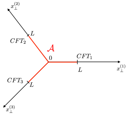
Figure 1: Junction of three CFTs and star shaped entangling surface ${\cal A}$.

We choose the entangling region ${\cal A}$ to enclose the interface symmetrically. For the $N$-junctions, we choose a symmetric star-shaped region (see figure 1 for an example of a $N=3$ junction) which extends the same distance in all half-spaces. The Ryu-Takayanagi prescription [4] states that the entanglement entropy is given by the area of a minimal surface in the bulk which encloses the boundary $\partial{\cal A}$ of the region ${\cal A}$ when it reaches the asymptotic AdS boundary. This prescription works straightforwardly for three dimensional spacetimes which asymptote to $AdS_{3}$. For the BPS junctions we have to generalize the prescription since the solution is a fibration of $AdS_{2}\times S^{2}$ over the upper half plane $\Sigma$. The minimal area surface for the holographic entanglement entropy is given by holding the $AdS_{2}$ time $t$ constant, setting $z=L$, and integrating over the two sphere $S^{2}$ and the Riemann surface $\Sigma$ (see figure 2). The entanglement entropy is then given by the area of this surface, and its expression may be read off using the metric of (2.1),

$$S_{e}={1\over{4G_{N}}}\int_{\Sigma}|dw|^{2}F_{-}^{2}\int_{S^{2}}\omega_{S^{2}}={\pi\over G_{N}}\int_{\Sigma}|dw|^{2}\left(\bar{\Lambda}\cdot\Lambda-2|\partial_{w}H|^{2}\right)$$ (3.1)

Here, $G_{N}$ is Newton’s constant. The second formula is obtained by integrating over $S^{2}$ in the first formula, and using the expressions for $F_{-}^{2}$ given in (2.1).

The above formula for the entanglement entropy $S_{e}$ is formal, as the integration over $\Sigma$ diverges due to the presence of the poles of $H$ and $\Lambda^{A}$ at the boundary of $\Sigma$. To regularize these divergences, we introduce a cutoff by removing a (half-) disk of coordinate radius $\varepsilon_{i}>0$ around the pole $x_{i}$ for all $i=1,\cdots,N$ (see figure 2).

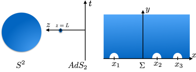
Figure 2: The $AdS_{2}\times S^{2}\times\Sigma$ space-time for $N=3$ junctions. The surface of minimal area is localized in $AdS_{2}$ at $z=L$, and encompasses all of $S^{2}\times\Sigma$.

Within the context of AdS/CFT, the cutoffs $\varepsilon_{i}$ at different poles must be related to the common UV-cutoff $\varepsilon$ of the dual CFT. In Appendix A, we shall provide a careful derivation of the corresponding relation,

$$\varepsilon_{i}^{2}={4\kappa_{i}\cdot\kappa_{i}\over\mu_{i}\cdot\mu_{i}}\,{\varepsilon^{2}\over L^{2}}$$ (3.2)

using the Fefferman-Graham expansion.

Convergence of the integral in (3.1) for large $|w|$ is guaranteed by the flux conservation formula of (2.6). Still, to evaluate the integrals of individual terms in (3.1) arising from the substitution of (2.2), it is convenient to also introduce a large $|w|$-cutoff $W$ so that $0<|w|<W$. The key integral needed to evaluate (3.1) is then given by,

$$\int_{\Sigma}{|dw|^{2}\over(w-x)(\bar{w}-y)}={\pi\over 2}\ln\left({W^{2}\over(x-y)^{2}+\varepsilon^{2}}\right)$$ (3.3)

along with its derivatives in $x$ and/or $y$. The result for the entanglement entropy becomes,

$$S_{e} = {\pi^{2}\over G_{N}}\,S_{R}+{\pi^{2}\over 2G_{N}}\sum_{i=1}^{N}\mu_{i}\cdot\mu_{i}\ln\left({\mu_{i}\cdot\mu_{i}L^{2}\over 8\varepsilon^{2}}\right)$$ (3.4)

$$S_{R} = \sum_{i=1}^{N}\sum_{j\not=i}\left({2\gamma_{i}\gamma_{j}-\kappa_{i}\cdot\kappa_{j}\over(x_{i}-x_{j})^{2}}+{\kappa_{j}\cdot\mu_{i}-\kappa_{i}\cdot\mu_{j}\over x_{i}-x_{j}}-{1\over 2}\mu_{i}\cdot\mu_{j}\ln{(x_{i}-x_{j})^{2}\over\gamma_{i}\gamma_{j}}\right)$$

It is immediate that $S_{e}$ and $S_{R}$ are invariant under $SL(2,{\mathbb{R}})$, which confirms that the AdS/CFT motivated regularization procedure of (3.2) is also $SL(2,{\mathbb{R}})$-invariant.

3.1 Extrema of the entropy solve all constraints

We establish a remarkable equivalence between configurations of the data $(x_{i},\gamma_{i},\kappa_{i},\mu_{i})$ which satisfy the constraints ${\cal E}_{i}^{(1)}={\cal E}_{i}^{(2)}=0$ for $i=1,\cdots,N$, and those which provide extrema of the entropy $S_{e}$. To formulate this equivalence precisely, we begin by spelling out the data that are kept fixed, and those that are to be varied in the extremization procedure.

The charge vectors $\mu_{i}$ are subject to overall charge conservation (2.6) and will be held fixed. The unit vector $\hat{\kappa}_{i}$ (satisfying $\hat{\kappa}_{i}\cdot\hat{\kappa}_{i}=1$) is taken to be orthogonal to $\mu_{i}$ and will also be held fixed. Relating the unit vector $\hat{\kappa}_{i}$ to $\kappa_{i},\mu_{i}$, and $\gamma_{i}$ by,

$$\kappa_{i}=\sqrt{2}\,\gamma_{i}\,\hat{\kappa}_{i}\hskip 72.26999pt\hat{\kappa}_{i}\cdot\mu_{i}=0$$ (3.5)

the constraints $\kappa_{i}^{2}=2\gamma_{i}^{2}$ and $\kappa_{i}\cdot\mu_{i}=0$ of (2.2) will automatically hold. In terms of the independent variables $x_{i},\gamma_{i},\hat{\kappa}_{i}$, and $\mu_{i}$ (the last subject to overall charge conservation), the reduced entropy $S_{R}$ of (3.4) is given by,

$$S_{R}=\sum_{i=1}^{N}\sum_{j\not=i}\left({2\gamma_{i}\gamma_{j}(1-\hat{\kappa}_{i}\cdot\hat{\kappa}_{j})\over(x_{i}-x_{j})^{2}}-2\sqrt{2}\,{\gamma_{i}\hat{\kappa}_{i}\cdot\mu_{j}\over x_{i}-x_{j}}-{1\over 2}\mu_{i}\cdot\mu_{j}\ln{(x_{i}-x_{j})^{2}\over\gamma_{i}\gamma_{j}}\right)$$ (3.6)

We shall now prove that the following variational problem precisely yields the constraint equations ${\cal E}_{i}^{(1)}={\cal E}_{i}^{(2)}=0$ of (2.2) and (2.2). Keeping the charges $\mu_{i}$ and the unit vectors $\hat{\kappa}_{i}$ fixed, and varying freely with respect to $x_{i}$ produces the equations ${\cal E}_{i}^{(1)}$. Varying freely with respect to $\gamma_{i}$ produces the equations ${\cal E}_{i}^{(2)}$. Indeed, from (3.6) one establishes the relations,

$${\partial S_{R}\over\partial x_{i}}=-2{\cal E}_{i}^{(1)}\hskip 72.26999pt\gamma_{i}{\partial S_{R}\over\partial\gamma_{i}}={\cal E}_{i}^{(2)}$$ (3.7)

where the identification $\kappa_{i}=\sqrt{2}\gamma_{i}\hat{\kappa}_{i}$ has been used to re-express the result of the variation of $S_{R}$ in the form on (2.2). It is remarkable that the constraints imposed on the solutions by the BPS conditions and the equation of motion can be viewed as conditions which follow from extremizing the holographic boundary entropy.

4 Kähler Structure of Moduli and Calabi’s Diastasis

In this section, we shall exhibit the Kähler structure which underlies the moduli space of half-BPS solutions with $N$ asymptotic $AdS_{3}\times S^{3}$ regions. We shall also introduce Calabi’s diastasis function in this setting, and relate it to the scalar fields in Type 4b supergravity. In subsequent sections, the entanglement entropy of certain subclasses of these solutions will be expressed with the help of the diastasis function.

4.1 Kähler structure of moduli

In Type 4b supergravity, the scalar field $V$ takes values in $SO(5,m)/\left(SO(5)\times SO(m)\right)$, a Grassmannian which is not generally Kähler (although it is $m=2$). For half-BPS solutions, however, supersymmetry requires $V$ to take values in the following submanifold,

$${\cal K}\equiv{SO(2,m)\over SO(2)\times SO(m)}$$ (4.1)

which is a Kähler Grassmannian for any value of $m$. The scalar field provides a smooth map $V:\Sigma\to{\cal K}$. Of central interest here are the values of $V$ at the points $x_{i}$ on $\partial\Sigma$, since all the solutions are specified uniquely by the data $x_{i},\gamma_{i},\kappa_{i},\mu_{i}$ at the $i=1,\cdots,N$ asymptotic $AdS_{3}\times S^{3}$ regions. We have learned, either from examination of the constraints (2.2) or from the variational solution provided in section 3.1, that the parameters $x_{i},\gamma_{i}$ are determined in terms of the data $\hat{\kappa}_{1},\cdots,\hat{\kappa}_{N}$ and $\mu_{1},\cdots,\mu_{N}$, subject to overall charge conservation (2.6) and the conditions $\hat{\kappa}_{i}^{2}=1$, $\mu_{i}^{2}>0$, and $\hat{\kappa}_{i}\cdot\mu_{i}=0$.

For each $i=1,\cdots,N$ the pair $(\hat{\kappa}_{i},\mu_{i})$, with $\hat{\kappa}_{i},\mu_{i}\in{\mathbb{R}}^{2+m}$ subject to the conditions $\hat{\kappa}_{i}^{2}=1$, $\mu_{i}^{2}>0$, and $\hat{\kappa}_{i}\cdot\mu_{i}=0$, projects to a unique point in the Kähler manifold ${\cal K}$. This follows from the fact that the two linearly independent vectors $\hat{\kappa}_{i}$ and $\mu_{i}$ uniquely define a 2-plane in ${\mathbb{R}}^{2+m}$, and thus a unique point in the Grassmannian ${\cal K}$. An explicit formula may be obtained for the canonical section $\sigma:{\cal K}\to SO(2,m)$ in terms of the scalar field $V$ by

$$\sigma_{AB} = \eta_{AB}-2V^{+}{}_{A}V^{-}{}_{B}-2V^{-}{}_{A}V^{+}{}_{B}$$ (4.2)

$$= \eta_{AB}-2\hat{\kappa}_{A}\hat{\kappa}_{B}-2\hat{\mu}_{A}\hat{\mu}_{B}$$

The canonical section $\sigma$ indeed takes values in $SO(2,m)$, as may be verified with $\sigma^{t}\eta\sigma=\eta$, and is clearly invariant under the action of $SO(2)\times SO(m)$, so that it is properly a map from the coset ${\cal K}$. Therefore, any pair $(\hat{\kappa}_{i},\mu_{i})$ projects to a unique point in ${\cal K}$. The converse, however, does not hold. First because given a value $\sigma_{i}$, only the 2-plane in which $\hat{\kappa}_{i}$ and $\mu_{i}$ live is determined, but the square $\mu_{i}^{2}$ and the angle distinguishing the direction of $\mu_{i}$ from the direction of $\hat{\kappa}_{i}$ are not determined by specifying a point $\sigma_{i}$ in ${\cal K}$.

Specifying $\mu^{2}_{i}\in{\mathbb{R}}^{+}$ in each asymptotic $AdS_{3}\times S^{3}$ region $i=1,\cdots,N$ amounts to specifying the radius of the $AdS_{3}$ or equivalently the central charge $c_{i}$ by the Brown-Henneaux formula. Adding an angle $\theta\in U(1)$ at each point $i$ completes the extra data into a point in ${\cal K}^{+}=SO(2,m)/SO(m)\times{\mathbb{R}}^{+}$, so that the full moduli space is given by,

$$({\cal K}^{+}_{1}\times\cdots\times{\cal K}^{+}_{N})_{\hbox{cc}}$$ (4.3)

where the subscript “cc” stands for enforcing the charge conservation relation of (2.6). This space naturally projects to the Kähler manifold ${\cal K}_{1}\times\cdots{\cal K}_{N}$ under the map provided by $\sigma$ as a function of the scalar field $V$.

4.2 Calabi’s diastasis in terms of supergravity fields

The purpose of this section is to compute the Kähler potential and evaluate Calabi’s diastasis function for the Kähler coset space ${\cal K}$. The starting point is the frame field $V$ of the $SO(2)\times SO(m)$ principal bundle over the coset $SO(2,m)/SO(2)\times SO(m)$, whose total space is the group $SO(2,m)$. It may be decomposed as follows,

$$V=\left(V^{(\rho,r)}{}_{A}\right)=\left(\matrix{V^{\rho}{}_{\alpha}&V^{\rho}{}_{a}\cr V^{r}{}_{\alpha}&V^{r}{}_{a}\cr}\right)$$ (4.4)

where $A=(\alpha,a)$ runs over the indices of the defining representation of $SO(2,m)$ with $\alpha=1,2$ and $a=6,\cdots,m+5$, while $\rho$ and $r$ run over the indices respectively of the defining representations of $SO(2)$ and $SO(m)$ with $\rho=1,2$ and $r=6,\cdots,m+5$. The group $SO(2,m)$ acts on $V$ by right-multiplication, while $SO(2)\times SO(m)$ acts by left-multiplication.

4.2.1 The Kähler form and metric

To compute the Kähler form $\omega_{\cal K}$ of ${\cal K}$, we identify $\omega_{\cal K}$ with the $SO(2)$ projection of the curvature of the right-invariant canonical connection $Q^{12}$ of this $SO(2)\times SO(m)$-bundle. Supergravity formulas gives us $Q=-Q^{t}$ in terms of the scalar field $V$ by the formula,

$$dV\,V^{-1}=\left(\matrix{Q&\sqrt{2}\,P\cr\sqrt{2}\,P^{t}&S\cr}\right)$$ (4.5)

and provide its curvature $\omega_{\cal K}=dQ^{12}$ in terms of $P$ by

$$\omega_{\cal K}=dQ^{12}=2\sum_{r}P^{1r}\wedge P^{2r}$$ (4.6)

In terms of the complex components of the scalar fields $V^{1,2}{}_{A}$ introduced in (2.4), the relevant algebraic relations are given by,

$$\eta^{AB}\,V^{\pm}{}_{A}V^{\mp}{}_{B} = 1$$

$$\eta^{AB}\,V^{\pm}{}_{A}V^{\pm}{}_{B} = 0$$ (4.7)

In terms of the variables $V^{\pm}{}_{A}$ the Kähler form $\omega_{\cal K}$ and the Kähler metric $ds^{2}_{\cal K}$ become,

$$\omega_{\cal K} = -i\eta^{AB}\,dV^{+}{}_{A}\wedge dV^{-}{}_{B}$$

$$ds^{2}_{\cal K} = \eta^{AB}\,dV^{+}{}_{A}\,dV^{-}{}_{B}$$ (4.8)

By construction, the Kähler form and metric are invariant under $SO(2,m)$.

4.2.2 The Kähler potential

To obtain the Kähler potential, it will be convenient to fix the gauge for the $SO(2)$ which acts on the indices $\pm$ of $V^{\pm}{}_{A}$. This will allow us to express the Kähler form, metric, and potential in terms of local complex coordinates. To do so in practice, we follow [30] and choose $V^{+}{}_{1}+iV^{+}{}_{2}$ to be real. The remaining complex coordinates are introduced as follows,

$$V^{+}{}_{1}={w+1\over 2\,\mathfrak{N}}\hskip 57.81621ptV^{+}{}_{2}=i{w-1\over 2\,\mathfrak{N}}\hskip 57.81621ptV^{+}{}_{5+s}={z^{s}\over\mathfrak{N}}$$ (4.9)

where $s=1,\cdots,m$. The equations of (4.2.1) determine $\mathfrak{N}$ in terms of the other variables, and give $w$ as a holomorphic function of the matrix $Z$ defined by $Z^{t}=(z^{1},\cdots,z^{m})$, so that,

$$2\,\mathfrak{N}^{2}=1+\left|Z^{t}Z\right|^{2}-2Z^{\dagger}Z\hskip 72.26999ptw=Z^{t}Z$$ (4.10)

The domain which represents the coset ${\cal K}$ in the variable $Z$ corresponds to $\mathfrak{N}>0$ along with the choice $Z^{\dagger}Z<1$, and is referred to as the Lie sphere,

$${\cal K}=\left\{Z\in{\mathbb{C}}^{m}~{}\hbox{such that}~{}Z^{\dagger}Z<{1\over 2}+{1\over 2}\left|Z^{t}Z\right|^{2}<1\right\}$$ (4.11)

Expressing the Kähler form of (4.2.1) in terms of these variables gives,

$$\omega_{\cal K}=d\left(id\ln\mathfrak{N}-i{(Z^{t}Z)\,Z^{\dagger}d\bar{Z}-Z^{t}d\bar{Z}\over\mathfrak{N}^{2}}\right)=-i\partial\bar{\partial}\ln\mathfrak{N}^{2}$$ (4.12)

with the help of the standard notations, $d=\partial+\bar{\partial}$ where $\partial=\sum_{s}dz^{s}{\partial\over\partial z^{s}}$. The Kähler potential $K$, which is defined by $\omega_{\cal K}=i\partial\bar{\partial}K$, is given by,

$$K(Z,\bar{Z})=-\ln\Big{(}1+|Z^{t}Z|^{2}-2Z^{\dagger}Z\Big{)}$$ (4.13)

4.2.3 Calabi’s diastasis function

Calabi’s diastasis function ${\cal D}(1,2)$ is defined for a pair of points in the Kähler manifold ${\cal K}$. We shall label these points by their complex coordinates $Z_{a}=(z_{a}^{1}\cdots z_{a}^{m})^{t}$ for $a=1,2$ and set $w_{a}=Z_{a}^{t}Z_{a}$. Calabi’s diastasis function is then defined by,

$${\cal D}(1,2)\equiv K(Z_{1},\bar{Z}_{1})+K(Z_{2},\bar{Z}_{2})-K(Z_{1},\bar{Z}_{2})-K(Z_{2},\bar{Z}_{1})$$ (4.14)

In terms of the coordinates $Z$, and the composite $w=Z^{t}Z$, it takes the following form,

$${\cal D}(1,2)=\ln{\left(1+w_{1}\bar{w}_{2}-2Z_{2}^{\dagger}Z_{1}\right)\left(1+w_{2}\bar{w}_{1}-2Z_{1}^{\dagger}Z_{2}\right)\over\left(1+\bar{w}_{1}w_{1}-2Z_{1}^{\dagger}Z_{1}\right)\left(1+\bar{w}_{2}w_{2}-2Z_{2}^{\dagger}Z_{2}\right)}$$ (4.15)

For $Z_{1}$ and $Z_{2}$ near the origin, the diastasis function reduces to ${\cal D}(1,2)\approx 2(Z_{1}-Z_{2})^{\dagger}(Z_{1}-Z_{2})$, and is proportional to the local Euclidean distance. More generally, it is an immediate consequence of the definition of the diastasis function in (1.1) that locally for $t_{2}\approx t_{1}$, the diastasis function is always approximated by the Euclidean distance. Globally, however, the diastasis function and the Riemannian distance between two points behave quite differently, both qualitatively and quantitatively. Key differences are that the diastasis function is neither always positive, not always obeys the triangle inequality.

4.2.4 Recasting the diastasis function in terms of the scalars $V$

To recast the diastasis potential in terms of the original supergravity scalars $V$, we begin by using the expression for the functions $2\mathfrak{N}_{a}^{2}=1+|w_{a}|^{2}-2Z_{a}^{\dagger}Z_{a}$. Eliminating the combinations in the denominator of the argument of the logarithm in (4.15), we find,

$${\cal D}(1,2)=\ln\left|{1+\bar{w}_{1}w_{2}-2Z_{1}^{\dagger}Z_{2}\over 2\,\mathfrak{N}_{1}\,\mathfrak{N}_{2}}\right|^{2}$$ (4.16)

We may now express Calabi’s diastasis in terms of the values $V(x_{i})$ and $V(x_{j})$ of the scalar field $V$ at a pair of points $i,j$, using (4.9) and their complex conjugates, and we find,

$${\cal D}(i,j)=\ln\left|\eta^{AB}V(x_{i})^{+}{}_{A}V(x_{j})^{-}{}_{B}\right|^{2}$$ (4.17)

Given the asymptotic values of the scalar field provided in (2.14), we obtain an equivalent relation directly in terms of the unit vector $\hat{\kappa}_{i},\hat{\kappa}_{j}$ and $\hat{\mu}_{i},\hat{\mu}_{j}$, as follows,

$${\cal D}(i,j)=\ln\Big{(}(\hat{\kappa}_{i}\cdot\hat{\kappa}_{j}+\hat{\mu}_{i}\cdot\hat{\mu}_{j})^{2}+(\hat{\kappa}_{i}\cdot\hat{\mu}_{j}-\hat{\mu}_{i}\cdot\hat{\kappa}_{j})^{2}\Big{)}$$ (4.18)

Note that the formulas for ${\cal D}(i,j)$ are manifestly invariant under $SO(2,m)$.

5 Entanglement entropy and diastasis of interfaces

In this section we will solve the constraints and evaluate the entanglement entropy for the simplest nontrivial case, namely the $N=2$ interface. In this case the general expression for the entanglement entropy (3.4) takes the following form,

$$S_{e} = {\pi^{2}\over G_{N}}\left(2{2\gamma_{1}\gamma_{2}-\kappa_{1}\cdot\kappa_{2}\over(x_{1}-x_{2})^{2}}+2{\kappa_{1}\cdot\mu_{2}-\kappa_{2}\cdot\mu_{1}\over x_{1}-x_{2}}-\mu_{1}\cdot\mu_{2}\ln(x_{1}-x_{2})^{2}\right.$$ (5.1)

$$\hskip 36.135pt\left.+{1\over 2}\mu_{1}^{2}\ln{\mu_{1}^{2}\over 4\kappa_{1}^{2}}+{1\over 2}\mu_{2}^{2}\ln{\mu_{2}^{2}\over 4\kappa_{2}^{2}}+{1\over 2}(\mu_{1}^{2}+\mu_{2}^{2})\ln{L^{2}\over\varepsilon^{2}}\right)$$

Note that charge conservation equates $\mu_{1}^{A}=-\mu_{2}^{A}$, which together with (2.2) implies

$$\kappa_{1}\cdot\mu_{2}=\kappa_{2}\cdot\mu_{1}=0.$$ (5.2)

The constraint ${\cal E}_{i}^{(2)}=0$ of (2.2) now takes the form,

$$\mu_{1}^{2}(x_{1}-x_{2})^{2}=4\gamma_{1}\gamma_{2}-2\kappa_{1}\cdot\kappa_{2}$$ (5.3)

and can be used to eliminate $x_{1}-x_{2}$ from the entaglement entropy (5.1). In addition we use (3.5) and (2.2) to replace $\kappa_{i}$ by the normalized $\hat{\kappa}_{i}$ for $i=1,2$ and (2.13) to replace $\mu_{1}^{2}=\mu_{2}^{2}$ by the central charge (which is the same on both sides due to charge conservation). The entanglement entropy becomes,

$$S_{e}={c\over 3}\ln{L\over\varepsilon}+{c\over 6}\big{(}1-\ln 2\big{)}+{c\over 12}\ln\left({1-\hat{\kappa}_{1}\cdot\hat{\kappa}_{2}}\right)^{2}$$ (5.4)

The first term in (5.4) is the universal contribution to the entanglement entropy which only depends on the central charge $c$, the length of the interval $L$, and the UV cutoff $\varepsilon$ [38, 39]. It has the same form whether or not an interface is present and can be removed by considering the difference between the entanglement entropy of pure $AdS_{3}$ and the interface space-time. The second term in (5.4) is non-universal and can be eliminated by a moduli independent rescaling of the cutoff. The third term in (5.4) is universal and present for a nontrivial interface. Hence, it may be identified with the $\mathfrak{g}$-function of the interface [6],

$$\ln\mathfrak{g}={c\over 12}\,\ln\left({1-\hat{\kappa}_{1}\cdot\hat{\kappa}_{2}}\right)^{2}$$ (5.5)

We can relate the $\mathfrak{g}$-function to the geometric diastasis function by using (4.18), and the fact that $\hat{\mu}_{1}\cdot\hat{\mu}_{2}=-1$, so that we find the following general expression for the $\mathfrak{g}$-function in terms of the central charge and the diastasis function of the interface,

$$2\ln\mathfrak{g}={c\over 6}\,{\cal D}(1,2)$$ (5.6)

The extra factor $c/6$ in front of the geometric diastasis function in (5.6) compared to (1.2) has the following explanation. The underlying CFT of the Type 4b $AdS_{3}\times S^{3}$ vacua is given by a symmetric product of ${\cal M}^{N}/S_{N}$ where ${\cal M}=T^{4}$ for the $m=5$ case and ${\cal M}=K_{3}$ for $m=21$. Since the CFT corresponding to a single ${\cal M}$ target space has central charge $c=6$ this implies that the number of copies of in the symmetric product $N=c/6$. Note that in a symmetric product all copies of the underlying ${\cal M}$ CFT are at the same point in the moduli space. Consequently the diastasis function for the ${\cal M}^{N}/S_{N}$ symmetric product CFT is given by $N$ times the diastasis function of the underlying CFT with target space ${\cal M}$. The example of [29] comprises a target space which is a single copy of $T^{2}$ and hence (1.2) holds without any additional factor.

To summarize, we have demonstrated the holographic version of the relation (1.2) between the $\mathfrak{g}$-function and the Calabi’s diastasis function, which was first discovered for the dual interface CFTs in [29].

6 Entanglement entropy and diastasis for 3-junctions

The goal of this section is two investigate whether the entanglement entropy (3.4) for the $3$-junction can be related to the diastasis function. For the case $N=3$ the constraint equations ${\cal E}_{i}^{(1)}=0$ in (2.2) imply the ${\cal E}_{i}^{(2)}=0$ constraint. Despite this simplification, the $N=3$ case is still considerably more difficult than the $N=2$ case of the interface, treated in the previous section, due in part to the fact that for a 3-junction, charge conservation does not force the charges $\mu^{A}$ to be parallel. The constraint equations form a non-linear system whose complete solution appears to require solving a quintic equation of general type.

To make progress, we recast the entropy and the constraints in terms of manifestly $SL(2,{\mathbb{R}})$-invariant variables, which are defined as follows,

$$y_{i}={\gamma_{i}(x_{j}-x_{k})\over(x_{i}-x_{j})(x_{i}-x_{k})}\hskip 72.26999pt\Delta_{ij}=\hat{\kappa}_{i}\cdot\hat{\kappa}_{j}-1$$ (6.1)

where $(i,j,k)$ in the first equation is a cyclic permutation of $(1,2,3)$. In these variables, the constraint equations become quadrics,

$$0=\mu_{i}^{2}+\sqrt{2}\hat{\kappa}_{i}\cdot(\mu_{j}-\mu_{k})y_{i}+4y_{i}y_{j}\Delta_{ij}+4y_{i}y_{k}\Delta_{ik}$$ (6.2)

Successively eliminating two of the three $y_{i}$ produces a polynomial equation in the third variable of degree 5, which does not lead to algebraic solutions. In terms of these variables, the entropy $S_{R}$ given in (3.6) takes the form,

$$S_{R} = -4y_{1}y_{2}\Delta_{12}-4y_{2}y_{3}\Delta_{23}-4y_{3}y_{1}\Delta_{31}+{1\over 2}\sum_{i=1}^{3}\mu_{i}^{2}\ln{1\over y_{i}^{2}}$$ (6.3)

$$+\sqrt{2}\hat{\kappa}_{1}\cdot(\mu_{3}-\mu_{2})y_{1}+\sqrt{2}\hat{\kappa}_{2}\cdot(\mu_{1}-\mu_{3})y_{2}+\sqrt{2}\hat{\kappa}_{3}\cdot(\mu_{2}-\mu_{1})y_{3}$$

Note that the variables $y_{i}$ now encompass the free $SL(2,{\mathbb{R}})$-invariant combinations of the variables $x_{i},\gamma_{i}$, so that extremization in $y_{i}$ indeed reproduces the constraint equations (6.2).

6.1 Solving for constrained charges

Although it does not appear possible to solve in simple terms for the 3-junction entropy in all generality, it is nonetheless possible to solve for a subclass of physically interesting charge arrangements. Under the assumption that the vector space spanned by the vectors $\kappa_{i}$ is orthogonal to the vector space spanned by the vectors $\mu_{i}$, the entropy may be obtained in explicit form, and in fact exhibits remarkable properties. This restricted case includes the physically important special situation where all 3-form charges $\mu_{i}$ are parallel to one another.

Concretely, the above orthogonality conditions are expressed by,

$$\hat{\kappa}_{i}\cdot\mu_{j}=0$$ (6.4)

for all $i,j=1,2,3$. The expression for the reduced entropy of (6.3) is given by,

$$S_{R}=-4y_{1}y_{2}\Delta_{12}-4y_{2}y_{3}\Delta_{23}-4y_{3}y_{1}\Delta_{31}+{1\over 2}\sum_{n=1}^{3}\mu_{n}^{2}\ln{1\over y_{n}^{2}}$$ (6.5)

while the constraints of (6.2) reduce to the equations,

$$0=\mu_{i}^{2}+4y_{i}y_{j}\Delta_{ij}+4y_{i}y_{k}\Delta_{ik}$$ (6.6)

where $(i,j,k)$ is a cyclic permutation of $(1,2,3)$. Solving for $y_{i}y_{j}$ with $i\not=j$ one finds,

$$y_{i}y_{j}={\mu_{i}\cdot\mu_{j}\over 4\Delta_{ij}}$$ (6.7)

Substituting into the entropy, we find,

$$S_{e} = {1\over 24}({c_{1}+c_{2}-c_{3}})\ln\left({\Delta_{12}\over\hat{\mu}_{1}\cdot\hat{\mu}_{2}}\right)^{2}+{1\over 24}({c_{2}+c_{3}-c_{1}})\ln\left({\Delta_{23}\over\hat{\mu}_{2}\cdot\hat{\mu}_{3}}\right)^{2}$$ (6.8)

$$+{1\over 24}({c_{3}+c_{1}-c_{2}})\ln\left({\Delta_{31}\over\hat{\mu}_{3}\cdot\hat{\mu}_{1}}\right)^{2}+{1\over 12}(c_{1}+c_{2}+c_{3})\Big{(}1+\ln{L^{2}\over 2\varepsilon^{2}}\Big{)}$$

Therefore the entanglement of the 3-junction with the restricted charge assignments $\hat{\kappa}_{i}\cdot\mu_{j}=0$ may be expressed in terms of the diastasis function for pairs, since we have,

$$\Delta_{ij}=-1-\hat{\mu}_{i}\cdot\hat{\mu}_{j}+e^{{\cal D}(i,j)/2}\,\hbox{sign}(\hat{\kappa}_{i}\cdot\hat{\kappa}_{j}+\hat{\mu}_{i}\cdot\hat{\mu}_{j})$$ (6.9)

A thorough discussion of the signs involved will be presented in the next section. Suffice it here to add the following explicit expression which suffice to evaluate the case where all flux charges $\mu_{i}$ are parallel to one another,

$$\hat{\mu}_{i}\cdot\hat{\mu}_{j}=-1 \ln\Delta_{ij}^{2}={\cal D}(i,j)$$

$$\hat{\mu}_{i}\cdot\hat{\mu}_{j}=+1 \ln\Delta_{ij}^{2}=\ln\left(2-e^{{\cal D}(i,j)/2}\,\hbox{sign}(\hat{\kappa}_{i}\cdot\hat{\kappa}_{j}+1)\right)^{2}$$ (6.10)

The first of these relations was used for the interface entropy.

7 Entropy and Calabi’s diastasis for $N$-junctions

For general $N>3$ junctions the system of constraint equations lends itself even less than for $N=3$ to a complete solution, as the constraints ${\cal E}_{i}^{(1)}=0$ in (2.2) now impose further non-trivial relations. Nonetheless, the system may be well-understood in terms of Calabi’s diastasis function for large physically relevant classes of data $\hat{\kappa}_{i},\mu_{i}$. Basically, the system lends itself to solution better when the dimension of the vector space spanned by the charge vectors $\mu_{i}$ is smaller. We begin by solving the case when the dimension is 1, and then produce extensions to low dimensions.

7.1 Parallel charge vectors $\mu_{i}$

One class of data $\hat{\kappa}_{i},\mu_{i}$ allows for complete solution in terms of Calabi’s diastasis function, namely when the charge vectors $\mu_{i}$ are parallel to one another for all $i=1,\cdots,N$,

$$\mu_{i}=\alpha_{i}\,\hat{\mu}_{1}\hskip 72.26999pt\sum_{i=1}^{N}\alpha_{i}=0\hskip 72.26999ptc_{i}={3\pi^{2}\,\alpha_{i}^{2}\over 2G_{N}}$$ (7.1)

Above we have indicated the overall charge conservation relation on the coefficients $\alpha_{i}$, as well as the relation resulting from (2.13) between the real coefficient $\alpha_{i}$ and the central charge $c_{i}$ of the $i$-th asymptotic region $AdS_{3}\times S^{3}$. Henceforth, we shall replace the data of the positive central charges $c_{i}$ by those of the coefficients $\alpha_{i}$. Clearly, $c_{i}$ determines $\alpha_{i}$ up to its sign, which will be important, and which will be denoted by $\hat{\alpha}_{i}=\hbox{sign}(\alpha_{i})$.

As a result of the assumption that $\mu_{i}$ are all parallel to one another, the orthogonality relations $\hat{\kappa}_{i}\cdot\mu_{i}=0$ imply the following orthogonality relations valid for all $i,j=1,\cdots,N$,

$$\hat{\kappa}_{i}\cdot\mu_{j}=0$$ (7.2)

The reduced entropy of (3.6) simplifies accordingly, and is given by,

$$S_{R}=\sum_{i=1}^{N}\sum_{j\not=i}\left({2\gamma_{i}\gamma_{j}(1-\hat{\kappa}_{i}\cdot\hat{\kappa}_{j})\over(x_{i}-x_{j})^{2}}-{1\over 2}\alpha_{i}\alpha_{j}\ln{(x_{i}-x_{j})^{2}\over\gamma_{i}\gamma_{j}}\right)$$ (7.3)

The parameters $\alpha_{i}$ are fixed by the central charges up to signs. We seek to eliminate the dependence on the data $\hat{\kappa}_{i}$ in favor of the diastasis function. The variables $x_{i}$ and $\gamma_{i}$ are to be determined by extremizing the entropy for given $\alpha_{i}$ and $\hat{\kappa}_{i}$, following section 3.1.

Calabi’s diastasis function, evaluated between pairs labeled by $i,j$ as in (4.18), then takes on a considerably simplified form under the assumption of (7.2), and we have,

$${\cal D}(i,j)=\ln\left(\hat{\kappa}_{i}\cdot\hat{\kappa}_{j}+\hat{\alpha}_{i}\,\hat{\alpha}_{j}\right)^{2}$$ (7.4)

Inverting this relation to obtain $\hat{\kappa}_{i}\cdot\hat{\kappa}_{j}$ in terms of ${\cal D}(i,j)$ and $\hat{\alpha}_{i}\hat{\alpha}_{j}$ requires care with sign issues. While the manifold of unit vectors $\hat{\kappa}_{i}$ in ${\mathbb{R}}^{2+m}$ with signature $(++-\cdots-)$ is connected, its submanifold of unit vectors orthogonal to a unit vector $\hat{\mu}_{1}$ of positive square is disconnected. Its two connected components may be distinguished by a sign $\hat{s}_{i}$, obtained as follows. Upon making an $SO(2,m)$ rotation, we may choose a canonical direction for the vector $\hat{\mu}_{1}$, and combine the first relation of (7.1) with (7.2), to parametrize $\kappa_{i}$ as follows,

$$\hat{\mu}_{1}=(1,0;{\bf 0})\hskip 72.26999pt\hat{\kappa}_{i}=\left(0,s_{i};~{}{\bf s}_{i}\right)\hskip 72.26999pts_{i}^{2}-{\bf s}_{i}^{2}=1$$ (7.5)

where $\hat{s}_{i}=\hbox{sign}(s_{i})$ while ${\bf s}_{i}$ is an arbitrary vector in ${\mathbb{R}}^{m}$. From this parametrization, the following inequality follows right away,

$$\hat{s}_{i}\hat{s}_{j}\,\hat{\kappa}_{i}\cdot\hat{\kappa}_{j}\geq 1$$ (7.6)

with equality only when $\hat{s}_{i}\,{\bf s}_{i}=\hat{s}_{j}\,{\bf s}_{j}$. Recasting the diastasis function in the form,

$${\cal D}(i,j)=\ln\Big{(}\hat{s}_{i}\hat{s}_{j}\hat{\kappa}_{i}\cdot\hat{\kappa}_{j}+\hat{s}_{i}\,\hat{s}_{j}\,\hat{\alpha}_{i}\,\hat{\alpha}_{j}\Big{)}^{2}$$ (7.7)

it is now straightforward and unambiguous to solve for the combination $\hat{s}_{i}\hat{s}_{j}\,\hat{\kappa}_{i}\cdot\hat{\kappa}_{j}$ which is always positive by (7.6). Extracting $\hat{\kappa}_{i}\cdot\hat{\kappa}_{j}$ from this result, we find,

$$\hat{\kappa}_{i}\cdot\hat{\kappa}_{j}=-\hat{\alpha}_{i}\hat{\alpha}_{j}+\hat{s}_{i}\hat{s}_{j}\,e^{{\cal D}(i,j)/2}$$ (7.8)

Substituting this result into (7.3) gives the desired expression for the reduced entropy in terms of Calabi’s diastasis function,

$$S_{R}=\sum_{i=1}^{N}\sum_{j\not=i}\left({2\gamma_{i}\gamma_{j}\left(1+\hat{\alpha}_{i}\hat{\alpha}_{j}-\hat{s}_{i}\hat{s}_{j}\,e^{{\cal D}(i,j)/2}\right)\over(x_{i}-x_{j})^{2}}-{1\over 2}\alpha_{i}\alpha_{j}\ln{(x_{i}-x_{j})^{2}\over\gamma_{i}\gamma_{j}}\right)$$ (7.9)

The solutions for $N=2$ and $N=3$ may be derived explicitly, and were given in the preceding sections. For $N\geq 4$, the constraint equations at present appear prohibitive.

7.2 Two-dimensional space of charge vectors $\mu_{i}$

We shall now proceed to the case where the space of charge vectors is 2-dimensional. To simplify the discussion, we limit attention to the case where this space is orthogonal to the vectors $\hat{\kappa}_{i}$ for all $i=1,\cdots,N$, or equivalently,

$$\hat{\kappa}_{i}\cdot\mu_{j}=0$$ (7.10)

for all $i,j=1,\cdots,N$. Using an $SO(2,m)$ rotation to set $\hat{\mu}_{1}$ to the direction given in (7.5), we see that the orthogonality of $\hat{\kappa}_{i}$ with $\hat{\mu}_{1}$ forces $\hat{\kappa}_{i}$ to take the form given in (7.5) for all $i=1,\cdots,N$. Using the residual $SO(1,m)$ group which leaves $\hat{\mu}_{1}$ invariant, we may choose any linearly independent unit charge $\hat{\mu}_{2}$ to take the form,

$$\hat{\mu}_{2}=(\alpha,\gamma;\beta,0\cdots 0)\hskip 72.26999pt\alpha^{2}+\gamma^{2}-\beta^{2}=1$$ (7.11)

We can have either $\beta=0$ when the vector restricted to $SO(1,m)$ has positive square, or $\gamma=0$ when it has negative square. The case $\gamma\not=0,\beta=0$ is ruled out by orthogonality to $\hat{\kappa}_{i}$, so that only the case $\gamma=0,\beta\not=0$ remains, and the first component of ${\bf s}_{i}$ must vanish. In summary, we have for all unit charge vectors,

$$\hat{\mu}_{j} = (\alpha_{j},0;\beta_{j},0\cdots,0)$$

$$\hat{\kappa}_{i} = (0,s_{i};0,{\bf s}_{i})$$ (7.12)

where $\alpha_{j}^{2}-\beta_{j}^{2}=1$, $\beta_{1}=0$, and ${\bf s}_{i}$ is an arbitrary vector in ${\mathbb{R}}^{m-1}$ with $s_{i}^{2}-{\bf s}_{i}^{2}=1$.

The diastasis function on pairs is now given as follows,

$${\cal D}(i,j)=\ln\left(\hat{\kappa}_{i}\cdot\hat{\kappa}_{j}+\alpha_{i}\alpha_{j}-\beta_{i}\beta_{j}\right)^{2}$$ (7.13)

Using care with the signs $\hat{s}_{i}$, we may invert this relation to find,

$$\hat{\kappa}_{i}\cdot\hat{\kappa}_{j}=-\alpha_{i}\alpha_{j}+\beta_{i}\beta_{j}+\hat{s}_{i}\hat{s}_{j}\,e^{{\cal D}(i,j)/2}$$ (7.14)

The reduced entropy now takes the form,

$$S_{R} = \sum_{i=1}^{N}\sum_{j\not=i}\left({2\gamma_{i}\gamma_{j}\over(x_{i}-x_{j})^{2}}\Big{\{}1+\alpha_{i}\alpha_{j}-\beta_{i}\beta_{j}-\hat{s}_{i}\hat{s}_{j}\,e^{{\cal D}(i,j)/2}\Big{\}}\right.$$ (7.15)

$$\hskip 72.26999pt\left.-{1\over 2}\sqrt{\mu_{i}^{2}\mu_{j}^{2}}\,(\alpha_{i}\alpha_{j}-\beta_{i}\beta_{j})\,\ln{(x_{i}-x_{j})^{2}\over\gamma_{i}\gamma_{j}}\right)$$

The physical value of the junction entropy is then obtained by the solution to the variational problem, exhibited in section 3.1, which gives $x_{i},\gamma_{i}$ in terms of the data $\hat{\kappa}_{i},\mu_{i}$.

To summarize, we see that the $N$-junction entropy is governed by Calabi’s diastasis function, along with the central charges $c_{i}=\mu_{i}^{2}$, but that a further dependence on the “angles” associated with the hyperbolic unit vectors $(\alpha_{i},\beta_{i})$ with $\alpha_{i}^{2}-\beta_{i}^{2}=1$ necessarily enters as well.

8 Entropy of a non-supersymmetric interface

The purpose of this section is to show that the interface entropy of a non-supersymmetric Janus solution is not given by the diastasis function but instead determined by the geodesic distance on the moduli space between the theories on the two sides of the interface. We include this calculation for two reasons. First, it provides an illustration that diastasis and supersymmetry are intimately linked (a point already made in [29]). Second, to the best of our knowledge, the calculation has not appeared earlier in the literature, and deserves attention in its own right.

The model we consider here is gravity in three-dimensional space-time with local coordinates $x^{\mu}$ and space-time metric $g_{\mu\nu}dx^{\mu}dx^{\nu}$ which is coupled to a nonlinear sigma model on a manifold $M$ with Riemannian internal metric. In terms of real local coordinates $\phi^{i}$ on $M$, the internal metric is given by $G_{ij}(\phi)d\phi^{i}d\phi^{j}$ and is considered fixed, and the action is a functional of the space-time metric $g_{\mu\nu}(x)$ and the fields $\phi^{i}(x)$, given by,

$$I[g,\phi]=\int d^{3}x\sqrt{g}\Big{(}R-2\Lambda-{1\over 2}G_{ij}(\phi)\partial_{\mu}\phi^{i}\partial^{\mu}\phi^{j}\Big{)}$$ (8.1)

where $\Lambda$ is the cosmological constant, and $g=-{\rm det}(g_{\mu\nu})$. Einstein’s equations are given by,

$$R_{\mu\nu}+\Lambda g_{\mu\nu}-{1\over 2}G_{ij}(\phi)\partial_{\mu}\phi^{i}\partial_{\nu}\phi^{j}=0$$ (8.2)

while the scalar field equations are given by,

$${1\over 2}\Big{(}{\partial\over\partial\phi_{k}}G_{ij}(\phi)\Big{)}\partial_{\mu}\phi^{i}\partial^{\mu}\phi^{j}-{1\over\sqrt{g}}\partial_{\mu}\Big{(}G_{ik}\sqrt{g}\,\partial^{\mu}\phi^{k}\Big{)}=0$$ (8.3)

We shall set $\Lambda=1$ and use the following Janus Ansatz in which the space-time metric is parameterized by an $AdS_{2}$ slicing and the scalars only depend on the slicing coordinate $y$,

$$ds^{2}=dy^{2}+f(y){dz^{2}-dt^{2}\over z^{2}}\hskip 72.26999pt\phi^{i}=\phi^{i}(y)$$ (8.4)

With this Ansatz the $tt$ and $zz$ components of (8.2) reduce to,

$$2-4f+{d^{2}f\over dy^{2}}=0$$ (8.5)

which is solved by the following family of functions dependent on a real parameter $\gamma$,

$$f(y)={1\over 2}\left(1+\sqrt{1-2\gamma^{2}}\cosh 2y\right)$$ (8.6)

The $AdS_{3}$ vacuum solution corresponds to setting $\gamma=0$, while $2\gamma^{2}=1$ corresponds to ${\mathbb{R}}\times AdS_{2}$. More generally, regular real solutions correspond to $2\gamma^{2}\leq 1$. The $yy$ component of the gravitational equation, and the scalar field equation may be similarly derived. Actually, it is illuminating to change variables from $y$ to $\lambda$ using the relation,

$$f(y){d\over dy}={d\over d\lambda}$$ (8.7)

The remaining equations then take the form,

$$G_{ij}(\phi)\,\dot{\phi}^{i}\dot{\phi}^{j}=2\gamma^{2}\hskip 72.26999pt\ddot{\phi}^{i}+\Gamma^{i}_{\;jk}\,\dot{\phi}^{j}\dot{\phi}^{k}=0$$ (8.8)

where the dot stands for differentiation with respect to $\lambda$, the Levi-Civita connection of the internal metric $G_{ij}$ is denoted by $\Gamma^{i}_{jk}$, and we continue to use the notation $\phi^{i}$ now for functions of the coordinate $\lambda$ instead of $y$.

8.1 Interface entropy

In this section calculate the interface entropy the non-supersymmetric Janus solution presented in the previous section. Following [34, 36], the interface entropy (or equivalently the $\mathfrak{g}$-function) can be related to the entanglement entropy of a region which encloses the interface symmetrically,

$$S_{e}={c\over 3}\ln{L\over\varepsilon}+\ln\mathfrak{g}$$ (8.9)

The holographic calculation of the interface entropy was performed in [34], and results in,

$$\ln\mathfrak{g}=-{c\over 6}\ln\sqrt{1-2\gamma^{2}}$$ (8.10)

Note that we have $g\to 1$ as $\gamma\to 0$, as this limit should indeed correspond to the the absence of the interface, and thus the vanishing of the interface entropy. Also note that reality of the entanglement entropy in (8.10) impose the same bound on $\gamma$ which had been imposed by the reality of the metric itself, namely $2\gamma^{2}\leq 1$.

The constraint equation in (8.8) relates the geodesic distance $\Delta\ell$ in the internal space of the non-linear sigma model to the deformation parameter $\gamma$,

$$\Delta\ell=\int d\lambda\sqrt{G_{ij}(\phi)\,\dot{\phi}^{i}\dot{\phi}^{j}}=\sqrt{2}\gamma\int d\lambda$$ (8.11)

The geodesic distance is evaluated as follows,

$$\Delta\ell=\sqrt{2}\gamma\int_{-\infty}^{+\infty}d\mu{1\over f(\mu)}=4\,{\rm tanh}^{-1}\left({1-\sqrt{1-2\gamma^{2}}\over\sqrt{2}\gamma}\right)$$ (8.12)

Solving for $\gamma$ in terms of $\Delta\ell$, one obtains,

$$\gamma={1\over\sqrt{2}}\tanh\left({\Delta\ell\over 2}\right)$$ (8.13)

Hence we obtain the interface entropy in terms of the geodesic distance $\Delta\ell$,

$$2\ln\mathfrak{g}={c\over 6}\,\ln\,\cosh\left({\Delta\ell\over 2}\right)^{2}$$ (8.14)

Note that the diastasis function coincides with the geodesic distance in the limit of infinitesimal separation [29] but differs for finite separations. Consequently, since the geodesic distance is different from the diastasis function the condition that the interface is BPS is essential in connecting $\ln\mathfrak{g}$ to the diastasis function.

Equation (8.13) implies that an expansion in small separation is equivalent to an expansion in small $\gamma$. The agreement of the diastasis and geodesic distance is consistent with [34] where it was found that the BPS and non-BPS interface $\mathfrak{g}$ functions agree at first order in an expansion in $\gamma$.

9 Summary and Discussion

The main results of this paper may be summarized as follows.

First, we have proven that the equivalence of interface entropy and Calabi’s diastasis function, which was derived for BPS interfaces in certain two dimensional CFTs in [29], continues to hold holographically for BPS interface solutions in six-dimensional Type 4b supergravity. Key to this equivalence is the fact that the moduli space of half-BPS interface solutions in Type 4b supergravity has an underlying Kähler manifold structure, which makes the appearance of Calabi’s diastasis function possible.

Second, we have extended the application of entanglement entropy to the case of a junction of $N\geq 3$ CFTs, where we have defined and carefully regularized an associated junction entropy. Using the holographic realization of these $N$-junctions in terms of Type 4b supergravity solutions, we have identified the moduli of the solutions, exhibited their underlying Kähler structure, and produced a variational formula for the evaluation of this junction entropy. For special arrangements of the flux charges, including when all the flux charges are parallel to one another, we have shown that the junction entropy may be represented as a sum of Calabi’s diastasis functions evaluated between the data associated with pairs of asymptotic $AdS_{3}\times S^{3}$ regions.

Third, we have shown that the interface entropy of a non-supersymmetric Janus solution to a 3-dimensional gravity-non-linear-sigma-model for a general internal Riemannian manifold $M$ is given in terms of the geodesic distance on $M$, and not in terms of any diastasis function. Unless $M$ is Kähler the diastasis function would not even exist. We interpret the results of this calculation as lending support to the assertion that the entropy-diastasis equivalence is intimately connected with supersymmetry.

The results in this paper leave open several interesting questions and avenues for future research, of which we list the following.

It would be instructive to find a way to relax the orthogonality condition (7.10) on the moduli of the $N$-junction solution, and to obtain the junction entropy for general charge assignments. Even for the 3-junction the general case appears considerably more complicated to solve algebraically, as it involves solving a quintic equation. It may be that a better parameterization, possibly along the lines of the light cone like variables used in [27], might help to solve the general case. Since the orthogonality condition were only imposed as a means of making the constraint equations solvable, it would be interesting to determine whether this condition has any physical meaning on the CFT side.

In Calabi’s original paper [30] the diastasis function is regarded as a potential. Specifically, the function ${\cal D}(1,2)$ is interpreted as the “potential” at point $2$ in the presence of a “source” at point $1$. A natural question emerging from this work is whether the $N$-junction entropy can be usefully interpreted as a potential in the presence of $N-1$ sources as well. One encouraging piece of supporting evidence is the fact that the constraints of (2.2) may be obtained equivalently from the variation of the entanglement entropy which, in turn, may be viewed as a zero force condition for a potential.

It would also be interesting to study the junction entropy on the CFT side along the lines of the work in [29] for interfaces. For example, we have already found that the holographic entanglement entropy for a 3-junction decomposes into a sum of diastasis functions between pairs, weighed by combinations of the three central charges. It would be valuable to determine whether such a structure can arise for BPS junctions on the CFT side as well.

Acknowledgements

We acknowledge useful conversations with Constantin Bachas, Michael Douglas, and Simon Gentle. This work was supported in part by National Science Foundation grants PHY-13-13986 and PHY-11-25915. One of us (ED) thanks the Kavli Institute for Theoretical Physics at the University of California, Santa Barbara for their hospitality and the Simons Foundation for their financial support while part of this work was being carried out.

Appendix A Regularization

In this appendix we present a careful holographic UV regularization and exhibit how the cutoff is imposed on the asymptotically $AdS_{3}\times S^{3}$ regions for the $N$-junction solutions.

A.1 Minimal area surface

In this subsection we adapt an argument [40, 41] concerning the minimal area hyper-surface for $AdS_{2}\times S^{2}$ fibrations, where the metric is given by (2.1). The metric of the $AdS_{2}$ factor is given by the unit radius Poincare patch metric

$$ds_{AdS_{2}}^{2}={dz^{2}-dt^{2}\over z^{2}}$$ (A.1)

The static minimal surface which is used to calculate the holographic entanglement entropy is independent of $t$, spans the sphere $S^{2}$ and extends over the Riemann surface $\Sigma$. Since the $SO(3)$ isometry of the two sphere is unbroken in the solution, the embedding is independent of the coordinates of $S^{2}$ and only depends on the local coordinates $w,\bar{w}$ of $\Sigma$, so that the embedding is completely specified by a single real-valued function $z(w,\bar{w})$ of $\Sigma$. The entanglement entropy $S_{e}$ is given by the area of the four-dimensional hyper-surface which minimizes the area with respect to the metric $G_{\rm ind}$ induced on $S^{2}\times\Sigma$,

$$S_{e} = {1\over 4G_{N}}\int_{S^{2}\times\Sigma}d^{4}\xi\sqrt{G_{\rm ind}}$$ (A.2)

$$= {\hbox{Vol}(S_{2})\over 4G_{N}}\int|dw|^{2}\,F_{-}^{2}\,\sqrt{1+{H^{2}\over F_{-}^{2}z^{2}}\left({\partial z\over\partial w}{\partial z\over\partial{\bar{w}}}\right)}$$

The square root on the second line above is manifestly bounded from below by 1, and this lower bound is uniquely attainted when the function $z$ is constant. Thus, $z=z_{0}$ constant is a solution and gives the absolute minimum for the area. The entanglement entropy on the hyper-surface of minimal area thus takes the form,

$$S_{e}={\hbox{Vol}(S_{2})\over 4G_{N}}\int|dw|^{2}\;F_{-}^{2}$$ (A.3)

The integration has divergent contributions coming from the asymptotic $AdS_{3}$ regions near $w=x_{n}$, $n=1,2,\cdots N$, which we shall regularize in the sequel.

A.2 Poincaré and $AdS_{2}$ slicing

In order to make a connection with the field theory result and extract the boundary entropy we have to carefully identify the cutoff $\varepsilon_{i}$ employed in the regularization of the entanglement entropy (A.3) with the UV cutoff in the field theory. The UV cutoff is defined by mapping the asymptotic metric near $w=x_{i}$ into a Fefferman-Graham coordinate system.

We start with an illustrative example mapping the three dimensional $AdS$ metric in Poincaré coordinates $(u,\eta,t)$, and metric,

$$ds^{2}=R^{2}\,{du^{2}+d\eta^{2}-dt^{2}\over u^{2}}$$ (A.4)

to new set of coordinates $(x,z,t)$

$$u={z\over\cosh x}\hskip 72.26999pt\eta=z\tanh x$$ (A.5)

In terms of these new coordinates $(x,z,t)$, the metric is the $AdS_{2}$ slicing of $AdS_{3}$,

$$ds^{2}=R^{2}\left(dx^{2}+\cosh^{2}x\,{dz^{2}-dt^{2}\over z^{2}}\right)$$ (A.6)

The Poincaré coordinates (A.4) are already in Fefferman-Graham form and the boundary is reached by taking $u\to 0$. The map (A.5) shows that the boundary $AdS_{2}$ slicing (A.6) has three components: the $AdS_{2}$ boundary $z\to 0$ which we identify with the interface and the two asymptotic regions $x\to\pm\infty$. For the latter regions and $z=z_{0}$ finite we can relate the cutoff in the Poincare coordinates $u=\varepsilon$ with the cutoff in $x$ by (A.5).

$$e^{-|x|_{\varepsilon}}={\varepsilon\over z_{0}}$$ (A.7)

For the solutions which are discussed in the present paper the situation is more complicated in several ways:

1. The three coordinates $x,z,t$ are accompanied by three additional coordinates parameterizing the two sphere and an additional (angular) slicing coordinate.

2. The metric (A.6) has two asymptotic regions $x\to\pm\infty$ and describes a configuration where two half spaces are glued together at an interface. For general $N>2$ our solutions describe junctions where $N$ half spaces are glued together.

3. The map (A.5) covers the complete Poincaré patch. Even for interface solutions a globally defined map is not known and the map has to be defined in patches.

In the following we shall address some of these issues with the primary goal to generalize the identification (A.7) to our solutions.

A.3 Regularization

To calculate the form of the metric near the $n$-th asymptotic region $w=x_{i}$, it is convenient to introduce the coordinate $w=x_{i}+e^{-x+i\theta}$, where the asymptotic $AdS$ region is reached by taking $x\to\infty$ and $\theta\in[0,\pi]$. The metric takes the following form

$$ds^{2}=\rho^{2}e^{-2x}(dx^{2}+d\theta^{2})+f_{1}^{2}{dz^{2}-dt^{2}\over z^{2}}+f_{2}^{2}ds_{S^{2}}^{2}$$ (A.8)

the asymptotic behavior of the metric near $w=x_{n}$ can be extracted from (2.1) and (2.1)

$$\rho^{2} \sim R_{i}^{2}\;e^{2x}\;\Big{(}1+e^{-x}\rho^{(1)}(\theta)+e^{-2x}\rho^{(2)}(\theta)+\cdots\Big{)}$$

$$f_{2}^{2} \sim R_{i}^{2}\;\sin^{2}\theta\Big{(}1+e^{-x}f_{2}^{(1)}(\theta)+e^{-2x}f_{2}^{(2)}(\theta)+\cdots\Big{)}$$

$$f_{1}^{2} \sim R_{i}^{2}\;{A_{i}^{2}\over 4}e^{2x}\Big{(}1+e^{-x}f_{1}^{(1)}(\theta)+e^{-2x}f_{1}^{(2)}(\theta)+\cdots\Big{)}$$ (A.9)

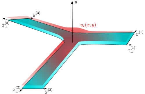
Figure 3: Fefferman-Graham cutoff surface $u=u_{\epsilon}(x,y)$ for $N=3$ junction.

Here the dots in the brackets denote terms which fall off faster than $e^{-2x}$ in the limit $x\to\infty$. The $AdS$ radius and the constant $A_{i}>0$ are expressed in terms of moduli associated with the $i$-th asymptotic region

$$R_{i}^{4}=2\mu_{i}\cdot\mu_{i}\hskip 72.26999ptA_{i}^{2}={16\kappa_{i}\cdot\kappa_{i}\over\mu_{i}\cdot\mu_{i}}$$ (A.10)

From the leading terms (A.3) we deduce that the metric takes an asymptotic $AdS_{3}\times S^{3}$ form. The subleading terms depend in general on the spherical slicing coordinate $\theta$. In the Fefferman-Graham the metric takes the following form,

$$ds^{2}_{FG}\sim R_{i}^{2}\Big{\{}{1\over u^{2}}\Big{(}du^{2}-g_{1}dt^{2}+g_{2}dx_{\perp}^{2}\Big{)}+g_{3}\Big{(}dy^{2}+\omega dx_{\perp}\Big{)}^{2}+g_{4}\sin^{2}yds_{S^{2}}^{2}\Big{\}}$$ (A.11)

Here $u$ is a Poincaré slicing coordinate where $u=0$ corresponds to the boundary of $AdS$ and the UV cutoff is defined by restricting the range $u>\varepsilon$. The coordinate $x_{\perp}$ denotes the distance from the junction and has a range $x_{\perp}\in[0,\infty]$. Scaling symmetry implies that the functions $g_{k}$ and $\omega$ depend only on $y$ and the combination $x_{\perp}/u$. In the limit $u\to 0$ the $g_{k}$ behave as,

$$\lim_{u\to 0}g_{k}\left({x_{\perp}\over u},y\right)=1,\;\;{k=1,2,3,4}\quad\quad\lim_{u\to 0}\omega\left({x_{\perp}\over u},y\right)=0$$ (A.12)

The maps between the $AdS_{2}$ slicing (A.8) and the Fefferman-Graham coordinate slicing (A.11) can be constructed in an asymptotic expansion in $e^{-x}$.

$${u\over z} = {2\over A_{i}}e^{-x}+k_{1}(\theta)e^{-2x}+\cdots$$

$${x_{\perp}\over z} = 1+l_{1}(\theta)e^{-x}+\cdots$$

$$y = \theta+m_{1}(\theta)e^{-x}+\cdots$$ (A.13)

As discussed [42, 40, 41] this coordinate map breaks down when $x_{\perp}$ becomes small compared to $u$. The region where the map is applicable is called a “Fefferman-Graham” (FG) patch”. For an N-junction all FG patches are smoothly joined to a central patch when $x_{\perp}\sim u$. While it is very hard to find such a map (see [40, 41, 42] for a discussion) we note that for the identification of the cutoff only map in the FG patch is needed since we can choose the location of the entangling surface $x_{\perp}=L$ to be much larger than the UV cutoff $u=\varepsilon$. It follows from (A.3) that in this case $x$ is large and we are safely in the FG patch.

The relation of the UV cutoff $\varepsilon$ and the radial integration cutoff in $\varepsilon_{i}$ in the $i$-th asymptotic $AdS_{3}\times S^{3}$ region is given by,

$$\varepsilon_{i} = e^{-x^{(i)}_{\varepsilon}}=A_{i}\,{\varepsilon\over 2L}$$ (A.14)

Plugging in the expression for $A_{i}$ give in (A.10) and squaring one arrives at,

$$\varepsilon_{i}^{2}={4\kappa_{i}\cdot\kappa_{i}\over\mu_{i}\cdot\mu_{i}}\left({\varepsilon\over L}\right)^{2}$$ (A.15)

Hence we have arrived at (3.2).

References

- [1] J. M. Maldacena, “The Large N limit of superconformal field theories and supergravity,” Adv. Theor. Math. Phys. 2 (1998) 231 [hep-th/9711200].
- [2] S. S. Gubser, I. R. Klebanov and A. M. Polyakov, “Gauge theory correlators from noncritical string theory,” Phys. Lett. B 428 (1998) 105 [hep-th/9802109].
- [3] E. Witten, “Anti-de Sitter space and holography,” Adv. Theor. Math. Phys. 2 (1998) 253 [hep-th/9802150].
- [4] S. Ryu and T. Takayanagi, “Holographic derivation of entanglement entropy from AdS/CFT,” Phys. Rev. Lett. 96 (2006) 181602 [hep-th/0603001].
- [5] S. Ryu and T. Takayanagi, “Aspects of Holographic Entanglement Entropy,” JHEP 0608 (2006) 045 [hep-th/0605073].
- [6] I. Affleck and A. W. W. Ludwig, “Universal noninteger ’ground state degeneracy’ in critical quantum systems,” Phys. Rev. Lett. 67 (1991) 161.
- [7] A. Karch and L. Randall, “Open and closed string interpretation of SUSY CFT’s on branes with boundaries,” JHEP 0106 (2001) 063 [hep-th/0105132].
- [8] C. Bachas, J. de Boer, R. Dijkgraaf and H. Ooguri, “Permeable conformal walls and holography,” JHEP 0206 (2002) 027 [hep-th/0111210].
- [9] C. Bachas and I. Brunner, “Fusion of conformal interfaces,” JHEP 0802 (2008) 085 [arXiv:0712.0076 [hep-th]].
- [10] J. Fuchs, M. R. Gaberdiel, I. Runkel and C. Schweigert, “Topological defects for the free boson CFT,” J. Phys. A 40 (2007) 11403 [arXiv:0705.3129 [hep-th]].
- [11] A. B. Clark, D. Z. Freedman, A. Karch and M. Schnabl, “Dual of the Janus solution: An interface conformal field theory,” Phys. Rev. D 71 (2005) 066003 [hep-th/0407073].
- [12] E. D’Hoker, J. Estes and M. Gutperle, “Interface Yang-Mills, supersymmetry, and Janus,” Nucl. Phys. B 753 (2006) 16 [hep-th/0603013].
- [13] D. Gaiotto and E. Witten, “Supersymmetric Boundary Conditions in N=4 Super Yang-Mills Theory,” J. Statist. Phys. 135 (2009) 789 [arXiv:0804.2902 [hep-th]].
- [14] D. Gaiotto and E. Witten, “Janus Configurations, Chern-Simons Couplings, And The theta-Angle in N=4 Super Yang-Mills Theory,” JHEP 1006 (2010) 097 [arXiv:0804.2907 [hep-th]].
- [15] D. Gaiotto, “Surface Operators in N = 2 4d Gauge Theories,” JHEP 1211 (2012) 090 [arXiv:0911.1316 [hep-th]].
- [16] N. Drukker, D. Gaiotto and J. Gomis, “The Virtue of Defects in 4D Gauge Theories and 2D CFTs,” JHEP 1106 (2011) 025 [arXiv:1003.1112 [hep-th]].
- [17] D. Bak, M. Gutperle and S. Hirano, “A Dilatonic deformation of AdS(5) and its field theory dual,” JHEP 0305 (2003) 072 [hep-th/0304129].
- [18] A. Clark and A. Karch, “Super Janus,” JHEP 0510 (2005) 094 [hep-th/0506265].
- [19] E. D’Hoker, J. Estes and M. Gutperle, “Exact half-BPS Type IIB interface solutions. I. Local solution and supersymmetric Janus,” JHEP 0706 (2007) 021 [arXiv:0705.0022 [hep-th]].
- [20] O. Lunin, “On gravitational description of Wilson lines,” JHEP 0606 (2006) 026 [hep-th/0604133].
- [21] E. D’Hoker, J. Estes and M. Gutperle, “Gravity duals of half-BPS Wilson loops,” JHEP 0706 (2007) 063 [arXiv:0705.1004 [hep-th]].
- [22] E. D’Hoker, J. Estes, M. Gutperle and D. Krym, “Exact Half-BPS Flux Solutions in M-theory. I: Local Solutions,” JHEP 0808 (2008) 028 [arXiv:0806.0605 [hep-th]].
- [23] E. D’Hoker, J. Estes and M. Gutperle, “Exact half-BPS Type IIB interface solutions. II. Flux solutions and multi-Janus,” JHEP 0706 (2007) 022 [arXiv:0705.0024 [hep-th]].
- [24] O. Lunin, “1/2-BPS states in M theory and defects in the dual CFTs,” JHEP 0710 (2007) 014 [arXiv:0704.3442 [hep-th]].
- [25] M. Chiodaroli, E. D’Hoker and M. Gutperle, “Open Worldsheets for Holographic Interfaces,” JHEP 1003 (2010) 060 [arXiv:0912.4679 [hep-th]].
- [26] M. Chiodaroli, M. Gutperle, L. -Y. Hung and D. Krym, “String Junctions and Holographic Interfaces,” Phys. Rev. D 83 (2011) 026003 [arXiv:1010.2758 [hep-th]].
- [27] M. Chiodaroli, E. D’Hoker, Y. Guo and M. Gutperle, “Exact half-BPS string-junction solutions in six-dimensional supergravity,” JHEP 1112 (2011) 086 [arXiv:1107.1722 [hep-th]].
- [28] M. Chiodaroli, E. D’Hoker and M. Gutperle, “Simple Holographic Duals to Boundary CFTs,” JHEP 1202 (2012) 005 [arXiv:1111.6912 [hep-th]].
- [29] C. P. Bachas, I. Brunner, M. R. Douglas and L. Rastelli, “Calabi’s diastasis as interface entropy,” arXiv:1311.2202 [hep-th].
- [30] E. Calabi,“Isometric Imbedding of Complex Manifolds”, Ann. Math. 58, 1 (1953).
- [31] L. J. Romans, “Selfduality for Interacting Fields: Covariant Field Equations for Six-dimensional Chiral Supergravities,” Nucl. Phys. B 276 (1986) 71.
- [32] N. Lashkari, M. B. McDermott and M. Van Raamsdonk, “Gravitational dynamics from entanglement ’thermodynamics’,” JHEP 1404 (2014) 195 [arXiv:1308.3716 [hep-th]].
- [33] T. Faulkner, M. Guica, T. Hartman, R. C. Myers and M. Van Raamsdonk, “Gravitation from Entanglement in Holographic CFTs,” JHEP 1403 (2014) 051 [arXiv:1312.7856 [hep-th]].
- [34] T. Azeyanagi, A. Karch, T. Takayanagi and E. G. Thompson, “Holographic calculation of boundary entropy,” JHEP 0803 (2008) 054 [arXiv:0712.1850 [hep-th]].
- [35] J. D. Brown and M. Henneaux, “Central Charges in the Canonical Realization of Asymptotic Symmetries: An Example from Three-Dimensional Gravity,” Commun. Math. Phys. 104 (1986) 207.
- [36] M. Chiodaroli, M. Gutperle and L. -Y. Hung, “Boundary entropy of supersymmetric Janus solutions,” JHEP 1009 (2010) 082 [arXiv:1005.4433 [hep-th]].
- [37] M. Chiodaroli, E. D’Hoker and M. Gutperle, “Holographic duals of Boundary CFTs,” JHEP 1207 (2012) 177 [arXiv:1205.5303 [hep-th]].
- [38] C. Holzhey, F. Larsen and F. Wilczek, “Geometric and renormalized entropy in conformal field theory,” Nucl. Phys. B 424 (1994) 443 [hep-th/9403108].
- [39] P. Calabrese and J. L. Cardy, “Entanglement entropy and quantum field theory,” J. Stat. Mech. 0406 (2004) P06002 [hep-th/0405152].
- [40] K. Jensen and A. O’Bannon, “Holography, Entanglement Entropy, and Conformal Field Theories with Boundaries or Defects,” Phys. Rev. D 88, 106006 (2013) [arXiv:1309.4523 [hep-th]].
- [41] J. Estes, K. Jensen, A. O’Bannon, E. Tsatis and T. Wrase, “On Holographic Defect Entropy,” JHEP 1405 (2014) 084 [arXiv:1403.6475 [hep-th]].
- [42] I. Papadimitriou and K. Skenderis, “Correlation functions in holographic RG flows,” JHEP 0410 (2004) 075 [hep-th/0407071].