One-dimensional $s$-$p$ optical superlattice

Abstract

The physics of one dimensional optical superlattices with resonant $s$-$p$ orbitals is reexamined in the language of appropriate Wannier functions. It is shown that details of the tight binding model realized in different optical potentials crucially depend on the proper determination of Wannier functions. We discuss the properties of a superlattice model which quasi resonantly couples $s$ and $p$ orbitals and show its relation with different tight binding models used in other works.

I Introduction

Cold atoms in optical lattices form a versatile medium for realizing different models of many-body systems, ranging from condensed matter to high-energy physics Jaksch05 ; Lewenstein07 ; hep . While originally the attention has been restricted to the standard simplest models (such as the celebrated Bose-Hubbard tight-binding Hamiltonian fisher89 ; jaksch98 ; Greiner02 ), soon there appeared a vast proliferation of research exploring unique possibilities offered by internal atomic structure (e.g. offering the possibility to create artificial gauge fields Lewenstein12 ; Taglia12 ; Taglia13 ) or by the flexibility of optical lattice potentials. In particular, superposition of laser standing waves with different wavevectors allows to create superlattice (SL) potentials. When these wavevectors are incommensurable, the resulting optical potential is pseudo-random, enabling studies of disordered systems Damski03 ; Fallani07 ; Fallani08 ; Zakrzewski09 . Small wavevector integer ratios lead to double- or triple-well periodic potentials, extensively studied due to their interesting properties Trotzky08 ; hemmerich . In particular, even simple one-dimensional potentials allow to observe interesting topological properties as the Zak-Berry phase Bloch13 or topological edge states Grusdt13 . Depending on the details of the model studied, different novel phases have been predicted Dhar2011 .

Most of these interesting studies assume a mapping between a continuous and a discrete version of the Hamiltonian, mapping accomplished by an appropriate choice of Wannier functions. Quite frequently, a discrete version of the Hamiltonian has been studied for arbitrary values of its parameters Dhar2011 ; dhar13 . The latter are, however, typically uniquely defined by the nature of the optical potentials and, possibly, interactions. Their determination requires a proper choice of the discrete basis representing the lattice. While for one dimensional sinusoidal potentials the procedure of constructing such a basis is well known from Kohn seminal works kohn , only recently a method to obtain the optimal basis of maximally localized Wannier functions for a double-well SL potential has been developed Modugno . This approach relies on the general scenario of Marzari and Vanderbilt Marzari97 ; Marzari12 and consists in designing a specific two-step gauge transformation of the Bloch functions for a composite two-band system.

Often one is interested in SL potentials which enable efficient coupling between the ground and excited bands, as exemplified in experiments of Hemmerich group hemmerich . The orbital physics LiuWu06 ; Wu06 ; Wu07 ; Wu08 ; Wu09 in such SL potentials Cai11 ; Li13 ; Li13a ; p-realization ; soltan lead to novel physical situations. As the method developed to find the optimal Wannier basis Modugno is valid for a generic set of two bands we apply it in this work considering in detail a SL case with a resonance between $s$ and $p$ orbitals in the neighboring sites. Besides, in Section III, we propose a simple analytic construction of Wannier-like functions valid at the exact $s-p$ resonance, showing that this leads to results which capture the essential features of the tight binding model obtained within the general method of ref. Modugno . The latter allows us to compute the tunneling amplitudes in a broad range of lattice depths also far from $s-p$ resonance, where seemingly the bands are decoupled, see Section IV. Finally, we compare the model obtained with different propositions discussed in the literature.

II Model

For simplicity we consider a purely one dimensional (1D) case with the Hamiltonian describing spinless atoms with contact interactions (described by effective coupling constant $g$) confined in the optical lattice potential $V(x)$:

$$\hat{\cal H}=\int\!\!\mathrm{d}x\hat{\Psi}^{\dagger}\left[-\frac{\hbar^{2}}{2M}\frac{\partial^{2}}{\partial x^{2}}+V\right]\hat{\Psi}+g\int\!\!\mathrm{d}x\hat{\Psi}^{\dagger 2}\hat{\Psi}^{2}.$$ (1)

The field operator $\hat{\Psi}(x)$ annihilates a boson at $x$. $\hat{\Psi}(x)$ is expanded in a single-particle basis of localized wave functions $f_{i}^{\alpha}(x)$:

$$\hat{\Psi}(x)=\sum_{i}\sum_{\alpha}\hat{a}^{\alpha}_{i}f_{i}^{\alpha}(x)$$ (2)

The operator $\hat{a}^{\alpha}_{i}$ annihilates a boson at site $i$, while the $\alpha$ index numbers the Bloch bands of the periodic potential $V(x)$. Performing the integrals in (1) results then in a (multiband) tight binding representation of the problem. We shall limit ourselves to relatively weak interactions for which the best localized basis states are single particle states determined only by the shape of the potential. We remark that in the limit of strong interactions the single particle basis may not be the optimal one Johnson09 ; Mering2011 ; Bissbort2012 ; Luhmann2012 ; Lacki2013a . Actually, despite its recent progress, the construction of a tight binding model for strong interactions remains an open problem.

The period-two SL potential is assumed of the form

$$V(x)=V_{0}\left[\sin^{2}(k_{L}x+\phi_{1})+\epsilon\sin^{2}(2k_{L}x+2\phi_{2})\right],$$ (3)

with $V_{0}$ being the amplitude and $k_{L}$ the wavevector of the laser beam. The case $\phi_{1}=\phi_{2}$ represents a rigid shift of the whole potential. Then the sign of $V_{0}$ as well as the parameter $\epsilon$ (assumed positive) determines the potential shape. $V_{0}<0$ corresponds to a collection of wells with the same minima and alternating heights of the barriers separating them Bloch13 ; Grusdt13 . Note that the period of the potential (3) is $d=\pi/k_{L}$, and the primitive cell contains a double well. Putting $\phi_{1}\neq\phi_{2}$ allows to modify both the minima and the maxima of the potential simultaneously Bloch13 . Positive values of $V_{0}$ for $\phi_{1}=\phi_{2}$ yield to wells of alternating depths enabling, for an appropriately chosen $\epsilon$, an efficient coupling between $s$-type states in the shallower wells and $p$-orbitals in the deeper wells. A similar scheme was used in hemmerich to effectively populate $p$-orbitals in a two-dimensional lattice.

Let us come now to the choice of suitable single-particle localized states $f_{i}^{\alpha}(x)$ in Eq. (2), which is the subject of this work. Generalized Wannier functions are expressed in terms of Bloch eigenfunctions as

$$w_{j\alpha}(x)=\sqrt{\frac{d}{2\pi}}\int_{\cal{B}}\!\!dk~{}e^{-ikja}\sum_{\beta=1}^{N}U_{\alpha\beta}(k)\psi_{\beta,k}(x)$$ (4)

where ${\cal{B}}$ is the first Brillouin zone. The unitary matrices must be continuous and periodic functions of $k$ in order to preserve the Bloch theorem. For a simple, say sinusoidal $V(x)$, the optimal basis is composed of exponentially localized single-band ($U_{\alpha\beta}(k)=e^{i\theta_{\alpha}(k)}\delta_{\alpha\beta}$) Wannier functions kohn . However, when the elementary cell contains two minima, as in the present case, single particle Wannier states are generally not localized in a single potential minimum. Besides, in the present work we shall choose the parameters $\epsilon$ and $V_{0}$ such that the lowest band is well separated from the others, with the next two lying very close and we will cosider the dynamics of the first and second excited bands. Consequently, as exposed in Modugno , we will consider the mixing of the relative two Bloch levels through a choice of the mixing matrix $U_{\alpha\beta}(k)$ built to minimize the spread of the corresponding Wannier functions. This procedure yields a localized $s$-like state in the shallow well and a $p$-like state in the deeper well. This configuration with two close lying bands is interesting owing to the fact that one may effectively populate the $p$-orbital (like in the two-dimensional experiment Olschlager13 ). This situation is also relevant for the realization of an effective Dirac dynamics with ultracold atoms in bichromatic optical lattices witthaut ; salger ; lopez-gonzalez .

To proceed, we use first the standard approach for periodic systems, i.e. diagonalization of the single-particle Hamiltonian as expressed in the recoil units of $E_{R}=\hbar^{2}k_{L}^{2}/2M$. Thus, in the following, energies (and the energy parameters such as the barrier height $V_{0}$) will be given in units of $E_{R}$ and the corresponding convenient unit of length will be $k_{L}^{-1}$. Also, from now on, we set $\phi_{1}=\phi_{2}=0$ in (3), corresponding to a potential configuration with degenerate maxima. The periodic part $u_{nk}(x)$ of the Bloch waves, $\psi_{nk}(x)=e^{ikx}u_{nk}(x)$, are obtained from a standard diagonalization procedure in Fourier space. Notice that they can be affected by arbitrary, uncorrelated phase factors for different quasimomenta $k$. Then, in order to obtain $u_{nk}(x)$ - continuous functions of $k$, we need to fix all the phases to zero at some point in $x$ space Modugno or equivalently, for a real matrix diagonalization (as possible for our simple potential) to choose the same signs of $u_{nk}(x)$ say at $x=0$.

III $s-p$ resonance

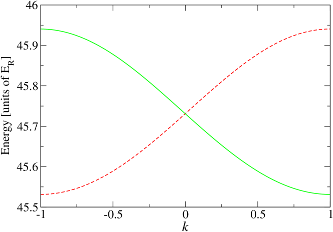
FIG. 1: Ccolor online) Energy bands for the double-well potential (3) with parameters $V_{0}=32E_{r}$, $\epsilon=2$ and $\phi_{1}=\phi_{2}=0$. The lowest energy band is not shown, the red (dashed) second band crosses with the green (solid) third band leading to a linear “relativistic” dispersion around $k=0$

Let us examine the resonant case. To this end, we take a particular $V_{0}$ and by diagonalizing the one-particle Hamiltonian for different values of $\epsilon$ we choose the one which makes the $2$nd and $3$rd Bloch bands cross (see Fig. 1). Then, by making a harmonic approximation for the wells, it is easy to find that the condition of resonance is $\epsilon=V_{0}/(16E_{R})$. Quite surprisingly, we have found numerically that this condition holds to a very good approximation also for relatively shallow wells, up to $V_{0}=16E_{R}$. Again, we remark that the use of the single-band approach (namely $U_{\alpha\beta}(k)=e^{i\theta_{\alpha}(k)}\delta_{\alpha\beta}$ in Eq. (4)) gives rise to Wannier functions $W_{0i}$ ($i=1,2,3$) well localized in a single well only for the states corresponding to isolated bands Modugno . For the present configuration, this is the case of $W_{01}$, whereas $W_{02}$ and $W_{03}$ have non-zero contributions both in the deeper and shallower wells (at resonance). Consequently, a non trivial mixing of the 2nd and 3rd bands is necessary. Remarkably, in this particular case, optimally localized states can be built from a simple analytic formula. In fact, let us consider the following Wannier-like states

$$W_{n}(x-R)=\frac{1}{\sqrt{2}}\int_{\mathcal{B}}dke^{-ikR}\psi_{nk}(x),$$ (5)

with $\mathcal{B}$ standing for the first Brillouin zone, so in our case: $d=\pi$ and $k\in[-1,1]$. This formula leads to the standard definition of the Wannier functions only when $R$ is a vector of the Bravais lattice, namely $R=R_{j}=j\pi$. Then, by using the following transformation

$$U=\frac{1}{\sqrt{2}}\left(\begin{array}[]{cc}1&1\\ -i&i\end{array}\right)$$ (6)

acting on the $n=2,3$ Bloch functions, and taking $R=(2j-1)\pi/2\equiv R^{(s)}_{j}$ for $s$-states and $R=j\pi\equiv R^{(p)}_{j}$ for $p$-states, we write (for the cell at $j=0$)

$$W_{s}(x) = \frac{1}{2}\int^{1}_{-1}\!\!\!dke^{+ik\frac{\pi}{2}}\Big{[}\psi_{2k}(x)+\psi_{3k}(x)\Big{]},$$ (7)

$$W_{p}(x) = \frac{i}{2}\int^{1}_{-1}\!\!\!dk\Big{[}-\psi_{2k}(x)+\psi_{3k}(x)\Big{]}.$$ (8)

Note that this transformation, along with the definition of the initial gauge for the Bloch states (see end of Sect. II), univocally defines this sets of Wannier functions. The functions $W_{s}$ and $W_{p}$ are localized in the minima of the shallow well ($x=-\pi/2$) and the deep one ($x=0$) respectively, see Fig. 2(a) foot1 . Both exhibit clear exponential fall-off, as seen in Fig. 2(b). For other cells the translation by $x=\pi$ (with integer $j$) applies, as required by the Bloch theorem. As it will be discussed in Sect. IV, this simple transformation captures the essential features of the general method of Ref. Modugno in describing the model and it leads to simple analytic expressions for the tunneling coefficients.

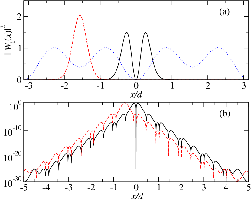
FIG. 2: (Color online) Top panel: two localized squared Wannier functions of the double-well potential (3) with parameters $V_{0}=32E_{r}$, $\epsilon=2$ and $\phi_{1}=\phi_{2}=0$. Functions $|W_{s}|^{2}$ (red dashed line) and $|W_{p}|^{2}$ (black solid line) come from Bloch functions transformed by (6). Dotted blue line depicts the lattice potential (not in scale). Bottom (b) panel shows the same Wannier functions in the logarithmic scale revealing their exponential localization within double precision arithmetics.

Then we introduce the following shorthand notation $W_{s}(x-R_{j})=\langle x|s_{j}\rangle$ and $W_{p}(x-R_{j})=\langle x|p_{j}\rangle$ for the Wannier-like functions belonging to the $j$-th cell, and denote with $E_{n}(k)$ the energy bands as indicated in Fig. 1. Then, it is straightforward to find the following expressions for the tunneling coefficients

$$J_{r} = -\langle s_{j}|\hat{H}_{0}|p_{j}\rangle=\frac{1}{2\pi}\int_{0}^{\pi}dk(E_{3}(k)-E_{2}(k))\sin\left({k}/{2}\right),$$

$$J_{l} = -\langle p_{j-1}|\hat{H}_{0}|s_{j}\rangle=-{J_{r}},$$

$$J_{s} = -\langle s_{j}|\hat{H}_{0}|s_{j+1}\rangle=-\frac{1}{2\pi}\int_{0}^{\pi}dk(E_{2}(k)+E_{3}(k))\cos(k),$$

$$J_{p} = -\langle p_{j}|\hat{H}_{0}|p_{j+1}\rangle=J_{s}.$$ (9)

With the choice of functions (7-8) the tunneling amplitudes are real. Notice that the tunneling amplitude, $J_{r}$ from $s$ $i$-site to the right (to $p_{i+1}$) has opposite sign to that corresponding to left hand side hop $J_{l}$ (due to the asymmetric character of the $p$ orbital). The tunneling amplitudes $J_{s,p}$ – between the same flavors $s$ and $p$ coincide at $s-p$ resonance.

One may adjust arbitrarily phases of Wannier functions. Changing the sign of every second double site (i.e. both $s$ and $p$ orbital functions) one may realize the “standard” system with $t$ amplitudes for nearest neighbor hopping and $t^{\prime}$ for next-nearest hopping (called often $t-t^{\prime}$ or $J_{1}-J_{2}$ model). This procedure, however, breaks partially the translational invariance of the system. To recover the translational invariance, the elementary cell has to be extended to four sites. Such a change of phases affects also the dispersion relation.

IV A general approach

As we have anticipated, the analytic transformation discussed in the previous section is designed specifically for the resonant case and cannot be applied to a generic situation. In the latter case, a general approach is represented by the so-called maximally localized Wannier functions (MLWFs) introduced by Marzari and Vanderbilt Marzari97 ; Marzari12 . They are obtained by generalizing the definition of Wannier functions for the case of a set of (almost) degenerate Bloch bands, and then minimizing their spread by means of an appropriate gauge transformation of the Bloch functions. By construction, this transformation is differentiable and is defined as periodic, in order to keep the periodicity of the Bloch functions. This method has been adopted by two of us for the lowest bands of 1D superlattice potential Modugno . It can also be applied straightforwardly to the present situation, yielding a set of MLWFs both at the $s-p$ resonance and in its vicinity, or in any situation in which there are two almost degenerate bands (well separated from the others). While the details of the approach have been presented in Modugno , here we briefly recall that it consists in using a specific two-step gauge transformation that makes vanishing the diagonal and off-diagonal gauge-dependent terms of the Wannier spread. Such a transformation is obtained by numerically solving a set of ordinary differential equations, with suitable boundary conditions. As a specific example, in the following we will fix $V_{0}=32E_{R}$ (for which the $s-p$ resonance occurs at $\epsilon=2$) to illustrate the typical behavior in the tight-binding regime.

Let us first discuss the resonant case, by comparing the general method with the results obtained by means of the analytic ansatz. First, observe that since the bands are degenerate at $k=0$ (see Fig. 1), the states in Eqs. (7-8) are built assuming that the second and the third bands are swapped for $k>0$, thus loosing the periodicity of the conventional Bloch bands. Alternatively, one could consider symmetric bands touching at $k=0$, with an additional $sgn(k)$ factor in the lower row of the mixing matrix, abandoning the periodicity and the continuity of the unitary transformation. This is a consequence of the fact that the specific choice of term $R$ in Eq. (5) for $s$ and $p$-like states is, as a matter of fact, equivalent to considering an effective lattice with half periodicity, that includes a single minimum in the elementary cell (notice that we are considering the case of degenerate maxima by having set $\phi_{1}=\phi_{2}=0$ in Eq. (3)). Remarkably, the Wannier-like states in Fig. 2 are almost coincident with those of the MLWFs obtained from the general procedure of Ref. Modugno . Also the corresponding tunneling amplitudes are well captured, as we will show in the following.

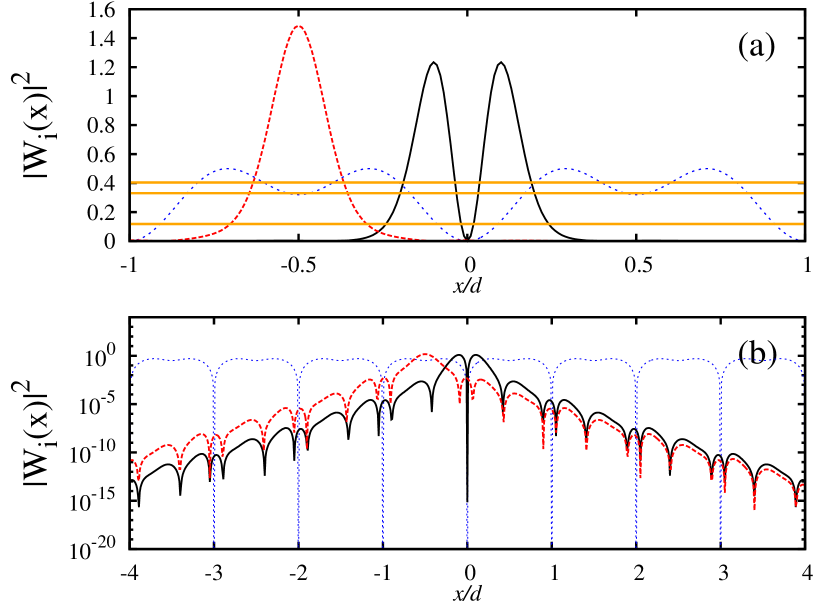
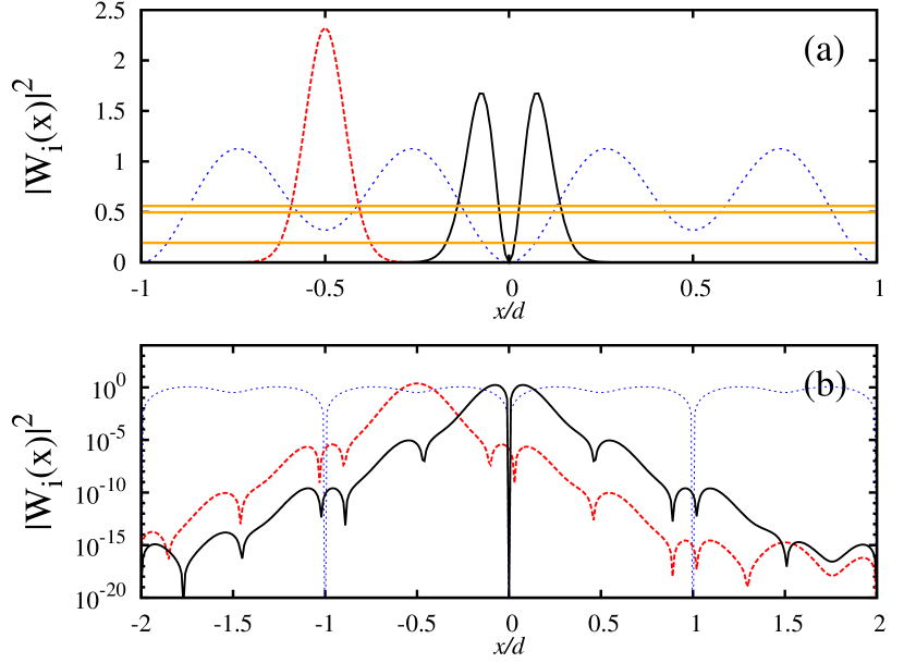
FIG. 3: (Color online) (a) Density plot of the $s-$ (red dashed line) and $p-$like (black solid line) MLWFs for $\epsilon=1$, corresponding to a large detuning from the resonance. The potential is represented by the dotted (blue) line, whereas the horizontal orange stripes represents the Bloch bands (on the same scale as the potential). (b) The same composite-band MLWFs are shown here in logarithmic scale. Note the exponential decay of the tails.

FIG. 4: (Color online) Same as above, but for $\epsilon=3$.

Let us now turn to the off-resonant case. As an example, in Figs. 4 and 4 we show the MLWFs for $\epsilon=1,3$, respectively. Each wave function is shown both in linear and logarithmic scale, in order to make evident that each of them is well localized around a single site, and to show the exponential falloff of their tails. Then, in Fig. 5a we show the behavior of the two onsite energies, namely $E_{s}\equiv\langle s_{j}|\hat{H}_{0}|s_{j}\rangle$ and $E_{p}\equiv\langle p_{j}|\hat{H}_{0}|p_{j}\rangle$, as a function of $\epsilon$. Note that below resonance $E_{s}>E_{p}$, whereas the situation is reversed above the resonance. The two on-site energies become degenerate exactly at $\epsilon=2$.

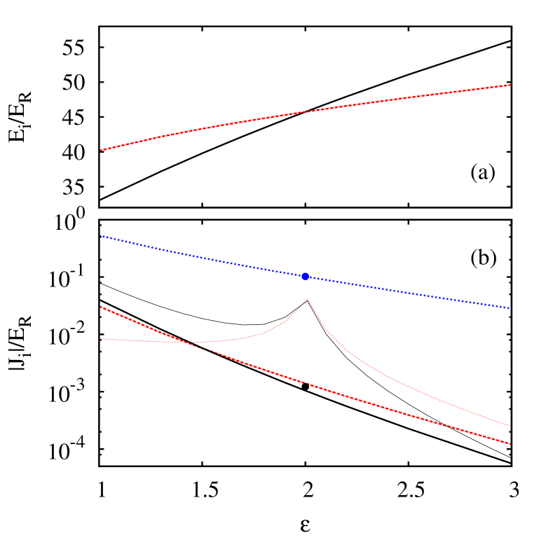
FIG. 5: (Color online) Onsite energies and tunneling amplitudes obtained from the composite-band MLWFs approach as a function of $\varepsilon$. (a) Onsite energies $E_{s}$ (black solid line) and $E_{p}$ (red dashed line). (b) Tunneling amplitudes: the blue (dotted) line corresponds to the amplitude $|J_{l}|=|J_{r}|$ for nearest-neighbor tunneling, i.e. between $s$ and $p$ orbitals; the black (solid) line corresponds to the $s-s$ tunneling amplitude $J_{s}$, while the red (dashed) line represents the $p-p$ tunneling $J_{p}$. Thin lines represents the values of $J_{s}$ and $J_{p}$ obtained from a single-band calculation (see text). The (blue and black) dots correspond to the prediction of the analytic expressions in Eq. (9) for the resonant case ($\varepsilon=2$).

Similarly, in Fig. 5b we show the behavior of the various tunneling amplitudes. They are characterized by a monotonic decrease with increasing $\epsilon$, as a consequence of the deepening of the potential wells. Note also that in this case the degeneracy between the $s-s$ and $p-p$ tunneling amplitudes takes place around $\epsilon=1.5$ and not at the resonance, as the tunneling rates are determined by the specific form of the Wannier functions, and not just by the value of the onsite energies. This is different from the result of the analytic approach, that predicts an exact degeneracy between $J_{s}$ and $J_{p}$ at the resonance (see the last equation in (9)). Nevertheless, apart from this detail, the analytic approach essentially captures the correct values of the tunneling coefficient at resonance. We also remark that, due to parity of $p$ orbital involved in $s-p$ hopping, the nearest neighbor tunneling amplitudes from a given site to the left and to the right have the same magnitude but opposite sign, namely $J_{l}=-J_{r}$, as already obtained for the analytic case discussed in the previous section.

Remarkably, that in the whole range of $\epsilon$ considered here, the amplitude of the nearest neighbor tunneling $J_{l/r}$ is an order of magnitude larger than the next-to-nearest neighbors tunneling amplitudes $J_{s}$ and $J_{p}$. Naively, this behavior is expected as the former corresponds to the hopping between neighboring wells. However, far from the resonance (e.g. at $\epsilon\simeq 1$ or $\epsilon\simeq 3$) one may also expect the usual single-band approach to provide Wannier functions that are well localized around each potential minima Modugno . Indeed, this is the case, as it will be shown in the following section. In this framework, the $s-$ and $p-$like Wannier states are orthogonal (they belong to different Bloch bands), and the nearest neighbor tunneling is exactly vanishing. Then, in order to clarify this apparent paradox, in the next section we will work out a thorough comparison between the single- and composite-band approaches.

V Far from the resonance: comparison with the single-band approach

Let us recall that proper single-band maximally localized Wannier functions can be constructed with the same approach a la Marzari and Vanderbilt discussed in the previous section. In this case it is necessary to minimize just the diagonal spread, as the off-diagonal one is vanishing by construction. In practice, this can be achieved by solving a set of simple ODEs for the phase $\phi_{n}(k)$ of the Bloch functions, corresponding to a $U(n)$ transformations ($n$ being the number of Bloch bands one is interested in) Modugno . Remarkably, the values of the phases $\phi_{n}(k)$ obtained from the numerical solution allow for a simple analytic approximation that consists in using Eq. (5) for $n=2,3$ and adjusting accordingly the centers $R$ of the Wannier functions to the bottoms of the corresponding wells, with an additional factor $sgn(k)$ for the $p$-state (that is centered in $x=0$). Indeed such a procedure, far from the resonance, leads to exponentially localized Wannier functions that are indistinguishable from those obtained numerically by minimizing their spread. We remark that this construction requires that the initial gauge for the Bloch functions is that defined at the end of Sec. II, and that each band is associated to the appropriate well. In particular, the $p$-type Wannier function corresponds to $n=2$ for $\epsilon$ below the resonance (i.e. $\epsilon<V_{0}/16$) and $n=3$ above it foot2 .

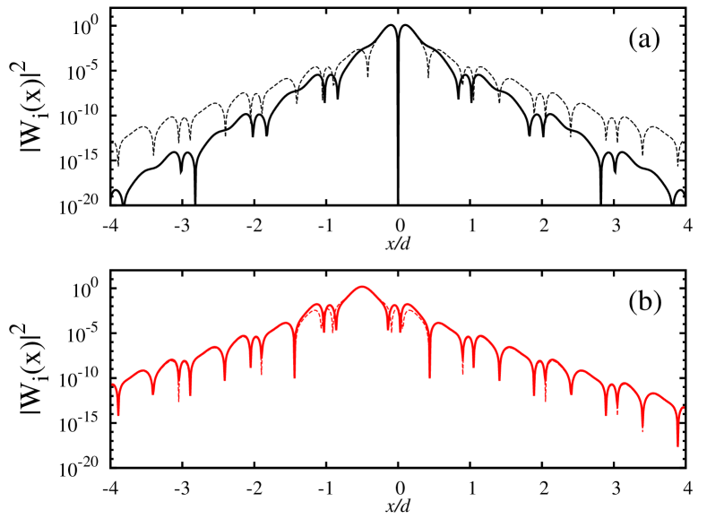
FIG. 6: (Color online) (a) Density plot of the $p-$like single-band Wannier functions (solid line) for $\epsilon=1$, compared with that obtained from the composite-band approach (dashed line). (b) The case of the $s-$like MLWF, as above.

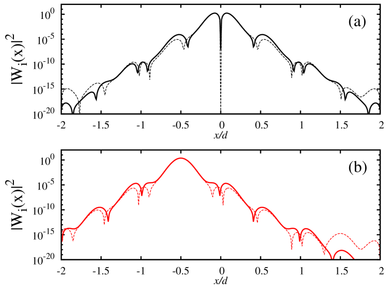
FIG. 7: (Color online) Same as Fig. 6, but for $\epsilon=3$.

As an example, the single-band Wannier functions obtained for $\epsilon=1,3$ are shown in Figs. 6, 7 in comparison with those obtained from the composite-band approach. Specifically, in these figures we show the modulus in logarithmic scale. In all cases, both sets of MLWFs show the same bulk behavior and are characterized by a nice exponential falloff of the tails. For $\epsilon=1$, where the two Bloch bands are well separated (see Fig. 4), the $p-$type Wannier function obtained from the single-band approach turns out to be more localized than that corresponding to composite bands (note the different slope of the exponential envelope), whereas the situation is reversed por the $s-$like function (note the first two side lobes). Instead, for $\epsilon=3$ - here the two bands are closer to each other - the composite-band MLWFs are more localized overall. In any case, we remark that the main difference between the two approaches resides in the structure of the Wannier functions as complex numbers (so far we have been showing just their modulus), that makes e.g. the $s$ and $p$ single-band states orthogonal. This is responsible for the very different structure of the tunneling coefficients, as shown in Fig. 5b. As a matter of fact, the single-band approach (that, we remind, is not suitable around the resonance as the Wannier functions occupy both wells Modugno ) corresponds to a picture with two sublattices one of type $s$ the other of type $p$ (with different tunneling rates within each sublattice), that are decoupled in the absence of interactions.

In the following, we will discuss which are the implications of the two pictures (single or composite bands), by considering first the structure of the single-particle spectrum and then the role played by interactions.

V.1 Single-particle spectrum

Let us recall that the single particle term of the tight-binding Hamiltonian up to nest-to-nearest neighbors takes the form

$$\hat{H}_{0} \simeq\sum_{\alpha=s,p}\sum_{j}E_{\alpha}\hat{n}_{j\alpha}-\sum_{\alpha=s,p}\sum_{j}J_{\alpha}(\hat{a}_{j\alpha}^{\dagger}\hat{a}_{(j+1){\alpha}}+h.c.)$$

$$-J\sum_{j}\left(\hat{a}_{js}^{\dagger}\hat{a}_{jp}-\hat{a}_{js}^{\dagger}\hat{a}_{(j-1){p}}+h.c.\right).$$ (10)

where $\hat{a}^{\dagger}_{j\alpha}$ ($\hat{a}_{j\alpha}$) represent creation (annihilation) operators associated to each lattice site, with $\alpha=s,p$.

The single-particle spectrum can be obtained by considering the following mapping to momentum space Modugno , $\hat{b}_{k\alpha}=\sum_{j}e^{i\pi kj}\hat{a}_{j\alpha}/\sqrt{2}$. Then, the single-particle Hamiltonian can be written as

$$\hat{H}_{0}=\sum_{\alpha\beta}\int_{\mathcal{B}}dkh_{\alpha\beta}(k)\hat{b}^{\dagger}_{k\alpha}\hat{b}_{k\beta},$$ (11)

with $h_{\alpha\beta}(k)$ defined as

$$h_{\alpha\beta}=\left(\begin{array}[]{cc}E_{s}-2J_{s}\cos(\pi k)&-J(1-e^{i\pi k})\\ -J(1-e^{-i\pi k})&E_{p}-2J_{p}\cos(\pi k)\end{array}\right).$$ (12)

For the single-band approach $J\equiv 0$, so that the dispersion relation takes the familiar form

$$E_{\alpha}^{sb}(k)=E_{\alpha}-2J_{\alpha}\cos(k\pi).$$ (13)

In the general case, the diagonalization of $h_{\alpha\beta}$ yields the following dispersion relation

$$E_{\pm}^{cb}(k) = E_{+}-2J_{+}\cos(k\pi)$$

$$\pm \sqrt{\left(E_{-}+2J_{-}\cos(k\pi)\right)^{2}+(2J)^{2}\sin^{2}(k\pi/2)},$$

with $E_{\pm}\equiv(E_{s}\pm E_{p})/2$, $J_{\pm}\equiv(J_{s}+J_{p})/2$.

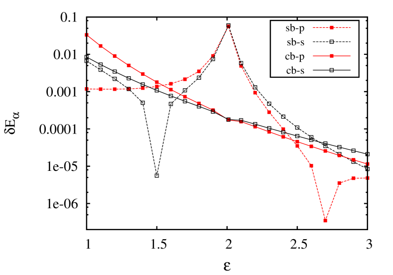
FIG. 8: (Color online) Plot of $\delta E_{\alpha}$ ($\alpha=s,p$, see text) as a function of $\varepsilon$, as obtained from the single- and composite-band approaches (indicated in the label as ‘sb’ and ‘cb’, respectively).

Then, the accuracy in reproducing the exact single particle Bloch spectrum can be measured by defining the following quantity Modugno

$$\delta E_{\alpha}\equiv\frac{1}{\Delta{E}_{\alpha}^{ex}}\sqrt{\frac{d}{2\pi}\int_{\cal{B}}dk\left[E_{\alpha}(k)-E_{\alpha}^{sb/cb}(k)\right]^{2}}$$ (15)

that represents the ratio of the quadratic spread between the exact Bloch spectrum $E_{\alpha}^{ex}(k)$ and that obtained from the single- or composite-band approach, to the Bloch bandwidth $\Delta{E}_{\alpha}^{ex}$. The behavior of $\delta E_{\alpha}$ as a function of $\varepsilon$ is shown in Fig. 8. This figure deserves a careful analysis. Close to $\varepsilon=1$, the nearest-neighbor approximation works accurately only in the single-band approach, and just for the lowest band (of type $p$). In the other cases, the inclusion of next-to-nearest tunneling terms would be required Modugno . Actually, in that limit the difference between the exact Bloch bands and those calculated with the nearest-neighbors tight-binding approach would be visible by eye. Then, it is evident starting from $\varepsilon=1.5$, the composite-band approach provides an increasing, very good accuracy in reproducing the single particle spectrum, thanks to the fact the the system enters a full tight-binding regime. Instead, the single-band approach is characterized by a mixed behavior, that is dramatically affected by the proximity of the resonance point, where it definitely fails. Only for $\varepsilon\gtrsim 2.2$ the single-band approach recovers a good accuracy level.

V.2 Interaction terms

Let us now turn to the interacting part of the many-body Hamiltonian. The full expression reads

$$\hat{H}_{int} =\frac{g}{2}\sum_{\{\alpha_{i}\}=s,p}\sum_{\{j_{i}\}}\hat{a}_{j_{1}\alpha_{1}}^{\dagger}\hat{a}_{j_{2}\alpha_{2}}^{\dagger}\hat{a}_{j_{3}\alpha_{3}}\hat{a}_{j_{4}\alpha_{4}}\cdot$$ (16)

$$\cdot\int dxW_{j_{1}\alpha_{1}}^{\ast}(x)W_{j_{2}\alpha_{2}}^{\ast}(x)W_{j_{3}\alpha_{3}}(x)W_{j_{4}\alpha_{4}}(x),$$ (17)

with $g$ being the coupling constant. The leading term is represented by usual Bose-Hubbard on-site interaction, namely

$$\hat{H}_{onsite}=\frac{1}{2}\sum_{\alpha=s,p}U_{\alpha}\sum_{j\alpha}\hat{n}_{j\alpha}\left(\hat{n}_{j\alpha}-1\right)$$ (18)

with $U_{\alpha}=g\int\!dx\left|W_{j\alpha}(x)\right|^{4}$. In addition to this, here we will consider also the effect of next-to-leading terms that couple nearest neighboring wells, i.e. $s$ and $p$ wells. They include a density-density interaction term

$$\hat{H}_{dens-dens}=\frac{g}{2}I_{2s2p}\cdot\hat{n}_{js}\hat{n}_{jp},$$ (19)

a density induced tunneling

$$\hat{H}_{dens-tun}=\frac{g}{2}I_{1s3p}\hat{a}_{js}^{\dagger}\hat{n}_{jp}\hat{a}_{jp}+\frac{g}{2}I_{3s1p}\hat{a}_{js}^{\dagger}\hat{n}_{js}\hat{a}_{jp}+(s\leftrightarrow p),$$ (20)

and the tunneling of pairs

$$\hat{H}_{pair-tun}=\frac{g}{2}I_{2s2p}\cdot\hat{a}_{js}^{\dagger}\hat{a}_{js}^{\dagger}\hat{a}_{jp}\hat{a}_{jp}+h.c.$$ (21)

In the previous expressions we introduced an intuitive notation for the integration integral within the $j$-cell indicating how many Wannier function of a given type enter into the integral

$$I_{iskp}\equiv\int dx(W_{js}(x))^{i}(W_{jp}(x))^{k},$$ (22)

taking into account that the Wannier functions can be chosen as real Brouder . Notice that there are also similar terms that couple $s-$states in the $j-th$ cell with $p-$states on the left, that is the $(j-1)$th cell. Observe, however, that the sign of the density dependent tunneling “to the left” is opposite to that “to the right” due to the asymmetry of the $p$-orbital, in parallel with the standard tunneling. A sketch of the various tunneling and interaction terms of the extended Bose-Hubbard model is shown in Fig. 9.

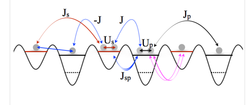
FIG. 9: (Color online) A sketch of the various tunneling and interaction terms of the extended Bose-Hubbard model. The color code is the same as that in Figs. 5 and 10. $J_{sp}$ schematically denotes two types of density dependent tunnelings, mediated by $s$ and $p$ orbitals densities. Remember that the nearest-neighbor tunneling coefficient $J$ is strictly vanishing within the single band approach.

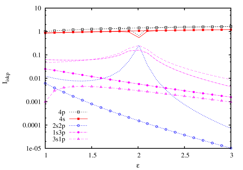
FIG. 10: (Color online) Plot of the (modulus of) the integrals $I_{iskp}$ characterizing the amplitude of various interaction terms of the extended Bose-Hubbard Hamiltonian. Lines with symbols correspond to the two-band approach, whereas plain lines refer to the single band case. Observe that the two-bands approach yields generally much smaller corrections to standard Bose-Hubbard terms, showing superiority over a single-band Wannier functions.

The relative weight of the various interaction terms listed above is shown in Fig. 10 where we present the behavior of the various integrals (in modulus) entering in their definition, as obtained from the both the single- and composite-band approaches (note that $I_{2s2p}=I_{2p2s}$). This figure shows that, as far as interactions are concerned, the composite-band model outperforms the single-band one, as the next-to-leading terms are significantly smaller in the former case. Notice also that (out of the resonant region) the values for on-site interaction given by the two approaches are al most indistinguishable. This is expected due to the very similar behavior of the bulk profiles of Wannier functions, see Figs. 6 and 7.

From Fig. 10 it is also evident that, in the range of $\epsilon$ considered here, the $s-p$ density-density interaction is completely negligible with respect to the on-site interaction. Similarly small is the pair tunneling contribution - as the integrals involved are exactly the same for contact interactions. These findings parallel general discussion for contribution of various interaction terms in the standard optical lattice - for a recent review see toberopp . Let us note, following toberopp , that the relative role of different terms may be different for long-range, e.g. dipolar, interactions which is, however, beyond the scope of this paper. On the other hand, the significance of the density induced tunnelings with respect to the leading order tunneling appearing in $\hat{H}_{0}$ depends on the value of the interaction constant $g$ and the lattice filling factors. When $g$ is small they can be safely neglected – see, however, toberopp and references therein.

VI Discussion

As mentioned in the introduction, superlattice potentials are often proposed to be employed for generating interesting model Hamiltonians. In particular, in this context, the so called $J_{1}-J_{2}$ (particularly for spins) or $t-t^{\prime}$ model was invoked with the non interacting part of the Hamiltonian being of the form

$$\hat{H}_{0}=-\sum_{i}\left(t\hat{a}_{i}^{\dagger}\hat{a}_{i+1}+t^{\prime}\hat{a}_{i}^{\dagger}\hat{a}_{i+2}+h.c.\right)+\sum_{i}E_{i}\hat{n}_{i}.$$ (23)

Here $t\equiv J_{1}$ corresponds to the nearest neighbor hopping while $t^{\prime}\equiv J_{2}$ is the next-nearest neighbor tunneling and $E_{i}$ stands for the on-site energy, common for all sites. By adding different form of interactions, different models are realized Dhar2011 ; dhar13 ; Li13a exhibiting frustration and different possible phases when arbitrary values of $J_{1}$ and $J_{2}$ parameters are assumed. It is often suggested that these models may be realized in one-dimensional superlattices. The present analysis, together with results of Modugno for lowest bands in optical superlattices, clearly indicates that it may be quite hard to observe the phases suggested in those papers. For lowest bands of superlattices Modugno the tunneling amplitudes are of the same sign while most interesting phases Dhar2011 ; dhar13 apper for opposite signs of $J_{1}$ and $J_{2}$. For the discussed here $s-p$ superlattice model, the tunnelings break left-to-right symmetry so mapping to $J_{1}-J_{2}$ model may be realised by changing the phases of Wannier functions breaking the translational invariance as discussed at the end of Sec. III for the resoant case. The similar approach is possible also out of the resonance. Still, as discussed extensively above, for the optimal, two-bands approach the nearest neighbour tunneling always dominates the next nearest terms. Thus it is impossible to reach $J_{1}\approx 2|J_{2}|$ region, most interesting for the appearance of Majumdar-Ghosh majumdar phase. The detailed discussion of possible phases in $s-p$ superlattice in the presence of interactions, also including density-dependent tunnelings deserves a separate investigation.

- (1) D. Jaksch and P. Zoller, Ann. Phys. 315, 52 (2005).
- (2) M. Lewenstein, A. Sanpera, V. Ahufinger, B. Damski, A. Sen, and U. Sen, Adv. Phys. 56, 243 (2007).
- (3) M. Endres, T. Fukuhara, D. Pekker, M. Cheneau, P. Schauss, C. Gross, E. Demler, S. Kuhr, and I. Bloch, Nature 487, 454, (2012).
- (4) M. P. A. Fisher, P. B. Weichman, G. Grinstein, D. S. Fisher, Phys. Rev. B 40, 546 (1989).
- (5) D. Jaksch, C. Bruder, J. I. Cirac, C. W. Gardiner, and P. Zoller, Phys. Rev. Lett. 81, 3108 (1998).
- (6) M. Greiner, O. Mandel, T. Esslinger, T. W. Hänsch, I. Bloch, Nature 415, 39 (2002).
- (7) M. Lewenstein, A. Sanpera, and V. Ahufinger, Ultracold Atoms in Optical Lattices: Simulating quantum many-body systems (Oxford University Press, Oxford, 2012).
- (8) L. Tagliacozzo, A. Celi, P. Orland, M. Lewenstein, preprint arXiv:1211.2704 (2012).
- (9) L. Tagliacozzo, A. Celi, A. Zamora, M. Lewenstein, Ann. Phys. 330, 160 (2013).
- (10) B. Damski, J. Zakrzewski, L. Santos, P. Zoller, and M. Lewenstein, Phys. Rev. Lett. 91, 080403 (2003).
- (11) D. Delande, and J. Zakrzewski, Phys. Rev. Lett. 102, 085301 (2009).
- (12) L. Fallani, J. E. Lye, V. Guarrera, C. Fort, M. Inguscio Phys. Rev. Lett. 98, 130404 (2007).
- (13) L. Fallani, C. Fort, M. Inguscio, Adv. At. Mol. Opt. Phys. 56, 119 (2008).
- (14) S. Trotzky, P. Cheinet, S. Fölling, M. Feld, U. Schnorrberger, A. M. Rey, A. Polkovnikov, E. A. Demler, M. D. Lukin, I. Bloch, Science 319, 295 (2008).
- (15) G. Wirth, M. Ölschläger, and A. Hemmerich, Nat. Phys. 7, 147 (2011).
- (16) M. Atala, M. Aidelsburger, J. T. Barreiro, D. Abanin, T. Kitagawa, E. Demler, I. Bloch, Nat. Phys. 9, 795 (2013).
- (17) F. Grusdt, M. Honing, and M. Fleischhauer, Phys. Rev. Lett. 110, 260405 (2013).
- (18) A. Dhar, T. Mishra, R. V. Pai, and B. P. Das, Phys. Rev. A 83, 053621 (2011)
- (19) A. Dhar, T. Mishra, R. V. Pai, S. Mukerjee, and B. P. Das, Phys. Rev. A 88, 053625 (2013).
- (20) W. Kohn, Phys. Rev. 115, 809 (1959).
- (21) M. Modugno, and G. Pettini, New J. Phys. 14, 055004 (2012).
- (22) N. Marzari, and D. Vanderbilt, Phys. Rev. B 56, 12847 (1997).
- (23) N. Marzari, A. A. Mostofi, J. R. Yates, I. Souza, D. Vanderbilt, Rev. Mod. Phys. 84, 1419 (2012).
- (24) W. V. Liu and C. Wu, Phys. Rev. A 74 , 013607 (2006).
- (25) C. Wu, W. V. Liu, J. Moore, and S. Das Sarma, Phys. Rev. Lett. 97, 190406 (2006).
- (26) C Wu, D. Bergman, L. Balents, and S. Das Sarma, Phys. Rev. Lett. 99, 070401 (2007).
- (27) C. Wu, Phys. Rev. Lett. 101, 186807 (2008) .
- (28) C. Wu, Mod. Phys. Lett. 23, 1 (2009).
- (29) Z. Cai and C. Wu, Phys. Rev. A 84, 033635 (2011).
- (30) X. Li, and W. V. Liu, Phys. Rev. A 87, 063605 (2013).
- (31) X. Li, E. Zhao, and W. V. Liu, Nat. Comm. 4, 1523 (2013).
- (32) T. Müller, S. Fölling, A. Widera, I. Bloch, Phys. Rev. Lett. 99, 200405 (2007).
- (33) P. Soltan-Panahi, D. -S. Lühmann, J. Struck, P. Windpassinger, and K. Sengstock, Nat. Phys. 8, 71 (2012).
- (34) P. R. Johnson, E. Tiesinga, J. V. Porto, and C. J. Williams, New J. Phys. 11, 093022 (2009).
- (35) A. Mering and M. Fleischhauer, Phys. Rev. A 83, 063630 (2011).
- (36) U. Bissbort, F. Deuretzbacher, and W. Hofstetter, Phys. Rev. A 86, 023617 (2012).
- (37) D.-S. Lühmann, O. Jürgensen, and K. Sengstock, New J. Phys. 14, 033021 (2012).
- (38) M. Łącki, D. Delande, and J. Zakrzewski, New J. Phys. 15, 013062 (2013).
- (39) M. Ölschläger, T. Kock, G. Wirth, A. Ewerbeck, C. Morais Smith, and A. Hemmerich, New. J. Phys. 15, 083041 (2013).
- (40) D. Witthaut, T. Salger, S. Kling, C. Grossert, and M. Weitz, Phys. Rev. A 84, 033601 (2011).
- (41) T. Salger, C. Grossert, S. Kling, and M. Weitz, Phys. Rev. Lett. 107, 240401 (2011).
- (42) X. Lopez-Gonzalez, J. Sisti, G. Pettini, and M. Modugno, Phys. Rev. A 89, 033608 (2014).
- (43) C. Brouder, G. Panati, M. Calandra, C. Mourougane, and N. Marzari, Phys. Rev. Lett. 98, 046402 (2007).
- (44) O. Dutta, M. Gajda, P. Hauke, M. Lewenstein, D.-S. Luehmann, B. A. Malomed, T. Sowinski, and J. Zakrzewski, arXiv:1406.0181 (2014).
- (45) C. K. Majumdar and D. K. Ghosh, J. Math. Phys. 10, 1388 (1969).
- (46) This construction works perfectly with a symmetric momentum grid that excludes the points .
- (47) Generally, since there are two choices one may either try both possibilities and see that only one works properly or use e.g. semiclassics to estimate in which sub-well of the superlattice one can expect lower-lying eigenstates.