Floquet Quantum Spin Hall Insulator in Cold Atomic Systems

Abstract

For cold atomic systems, varying the optical lattice potential periodically provides a general and simple way to drive the system into phases with nontrivial topology. Besides its simplicity, this driving approach, compared to the usual driving approach by exerting an external electromagnetic field to the static system, has the merit that it does not break the original static system’s time-reversal symmetry at any given time. Based on this approach, we find that a trivial insulator with time-reversal symmetry can be driven into a Floquet quantum spin Hall insulator. This novel state of matter can stably host one or two pair of gapless helical states on the same boundary, which suggests this state is not a simple analog of the quantum spin Hall insulator. The effect of a time-reversal-symmetry-breaking periodic perturbation, the stability of the novel states, and this new driving approach to a system without time-reversal symmetry are discussed.

Introduction.— In the past few years, the theoretical predictions C. L. Kane1 ; C. L. Kane2 ; B. A. Bernevig and the experimental observations M. Konig ; D. Hsieh of topological insulator have stimulated strong and continuous interest in predicting new materials and systems with topological phases due to their potential application in spintronic and topological quantum computation A. Kitaev .

Topological phases exist in every dimension A. P. Schnyder ; A. Y. Kitaev , however, it is found that the number of real static systems with topological properties is quite limited. This limitation triggers new proposals to engineer systems with topological properties. One such proposal that time-periodically driven systems can host topological characteristics, the so-called Floquet approach T. Kitagawa1 ; N. H. Lindner , recently has attracted great attention J.-I. Inoue ; Z. Gu ; Ferenc Simon ; G. C. Liu ; G. Platero ; D. L. Bergman ; A. A. Reynoso ; Y. T. Katan ; D. E. Liu ; A. Kundu ; M. Lababidi ; P. M. Perez-Piskunow ; A. G. Grushin , and has been demonstrated by the direct observation of protected edge modes in photonic crystals M. C. Rechtsman ; T. Kitagawa2 . The great interest arisen are not only this approach can drive a topologically trivial system to be topologically nontrivial but also the driven systems can exhibit unique topological properties without an analog in static systems T. Kitagawa3 ; M. S. Rudner , such as the Floquet Majorana fermions with quasienergy $\epsilon=\pi/T$ L. Jiang .

For solid state systems, currently the general way to drive the system from a trivial phase into a topological phase is by introducing a time periodic external electromagnetic field to the original static system, like shining light on a conventional insulator. This method is simple and easy to control, however, it has a drawback that if the external field, like an oscillating magnetic field, directly couples with the spin, it usually breaks the time-reversal symmetry of a spinful fermionic system in the sense: $\mathcal{T}\hat{H}_{0}(-k)\mathcal{T}^{-1}=\hat{H}_{0}^{*}(k)$ but $\mathcal{T}\hat{H}(-k,t)\mathcal{T}^{-1}\neq\hat{H}^{*}(k,t)$ for any given $t$ at which the external field is nonzero, where $\hat{H}_{0}(k)$ is the original static Hamiltonian and $\hat{H}(k,t)$ is the driven Hamiltonian, $\mathcal{T}=i\sigma_{y}\mathcal{K}$. The consequence of this drawback is that if the external field only induces driving terms that break the time-reversal symmetry, a topologically trivial system with time-reversal symmetry can never be driven to be topologically nontrivial. To avoid this drawback, therefore a general driving method which guarantees inducing terms that do not break the time-reversal symmetry is favored.

For cold atomic systems, we find there exists such a general and simple method to drive the system periodically without breaking the time-reversal symmetry if the original static system is time-reversal invariant. The method is varying the optical potential periodically, which means $V({\bf r},t)=V({\bf r},t+T)$. A direct consequence of periodically varying the optical lattice is that the hopping amplitude of a tight-binding model will turn to be periodic. For a time-reversal invariant static system, the hopping amplitude turning to be time-periodic does not break the time-reversal symmetry. As a consequence, for a time-reversal invariant insulator, the edge states driven up are always helical, the same as the Quantum Spin Hall (QSH) insulator C. L. Kane1 ; C. L. Kane2 ; B. A. Bernevig (for a time-reversal invariant superconductor or superfluid, the picture is similar and therefore we restrict ourself to insulator in this work). For the sake of accuracy, here we name systems hosting such driven-up helical edge states as Floquet Quantum Spin Hall (FQSH) insulator.

Theoretical model with time-reversal symmetry— We consider a cold atomic realization of the time-reversal symmetric Kane-Mele model in a hexagonal optical lattice. The Hamiltonian is given by C. L. Kane1

$$H_{KM}=J\sum_{<i,j>}c^{{\dagger}}_{i}c_{j}+i\lambda_{SO}\sum_{<<i,j>>}\nu_{ij}c^{{\dagger}}_{i}\sigma_{z}c_{j}+\lambda_{v}\sum_{i}\xi_{i}c^{{\dagger}}_{i}c_{i}.$$ (1)

The first term denotes the nearest-neighbor hopping process. The second term is the mirror symmetric spin-orbit interaction which involves spin-dependent next-nearest-neighbor hopping. $\nu_{ij}$ takes value $1$ (or $-1$) when the path $i\rightarrow j$ is contourclockwise (or clockwise). The third term is a staggered sublattice potential ($\xi_{i}=\pm$), which are included to control the phase.

For a hexagonal lattice, the optical lattice potential takes the form L.-M. Duan

$$V({\bf r},t)=\sum_{i=1,2,3}V_{i}(t)\sin^{2}[k_{L}(x\cos\theta_{i}+y\sin\theta_{i})+\frac{\pi}{2}],$$ (2)

where $\theta_{1}=\pi/3$, $\theta_{2}=2\pi/3$ and $\theta_{3}=0$. $k_{L}$ is the optical wave vector. Here we consider a hexagonal optical lattice with isotropic driving, $i.e.$ $V_{i}(t)=V_{0}+V_{D}\cos(\omega t)$. With such a driving, the hopping amplitudes correspondingly vary with time periodically: $J(t)=J+J_{D}\cos(\omega t)$, $\lambda_{SO}(t)=\lambda_{SO}+\lambda_{SO,D}\cos(\omega t)$. Then the time-dependent Hamiltonian can be decomposed as $H(t)=H_{KM}+H_{D}\cos(\omega t)$. $H(t)$ is time-periodic and $H_{D}$ is given by

$$H_{D}=J_{D}\sum_{<i,j>}c^{{\dagger}}_{i}c_{j}+i\lambda_{SO,D}\sum_{<<i,j>>}\nu_{ij}c^{{\dagger}}_{i}\sigma_{z}c_{j}.$$ (3)

$H_{D}$ has the same form as $H_{KM}$ except the absence of a corresponding term to $\lambda_{v}$ (in fact, even if we include such a corresponding term, the conclusion is not affected), and therefore does not break the time-reversal symmetry, and the total Hamiltonian $H(t)$ still hold the time-reversal symmetry.

The single-particle Schrödinger equation associated with this time-dependent Hamiltonian is:

$$[\mathcal{H}(\mathbf{k},t)-i\partial_{t}]\Psi(\mathbf{k},t)=0,\,\text{with}\,\mathcal{H}(\mathbf{k},t+T)=\mathcal{H}(\mathbf{k},t).$$ (4)

where $\mathcal{H}(\mathbf{k},t)$ is the form of $H(t)$ in momentum space. According to the Bloch-Floquet theory, the wave function satisfying Eq.(4) can be expressed as $\Psi(\mathbf{k},t)=\text{e}^{-i\varepsilon_{\mathbf{k}}t}\Phi(\mathbf{k},t)$ with the Floquet states $\Phi(\mathbf{k},t+T)=\Phi(\mathbf{k},t)$ and the Floquet equation $[\mathcal{H}(\mathbf{k},t)-i\partial_{t}]\Phi(\mathbf{k},t)=\varepsilon_{\mathbf{k}}\Phi(\mathbf{k},t)$. The parameter $\varepsilon$, called the quasienergy, is uniquely defined up to integer multiples of $\omega=2\pi/T$. Similar to the crystal momentum of a system with discrete translation symmetry, the quasienergy can be thought of as a periodic variable defined on a quasienergy Brillouin zone $-\pi/T<\varepsilon\leq\pi/T$.

Although there are many different (but equivalent) ways to compute the topological invariant for a time-reversal symmetric insulator Z. Wang , to the best of our knowledge, a direct way to calculate the topological invariant for a time-reversal symmetric driven model is still lacked. To determine the topological property of the time-dependent Hamiltonian, here we use the ‘repeated zone analysis’ M. S. Rudner . The first step is to expand the Floquet states, $\Phi(\mathbf{k},t)=\sum_{m}\phi_{m}(\mathbf{k})\text{e}^{im\omega t}$. The coeffcients $\phi_{m}(\mathbf{k})$ satisfy the time-independent eigenvalue equation

$$\sum_{m^{{}^{\prime}}}\mathcal{H}_{m,m^{{}^{\prime}}}(\mathbf{k})\phi_{m^{{}^{\prime}}}(\mathbf{k})=\varepsilon_{\mathbf{k}}\phi_{m}(\mathbf{k}),$$ (5)

where the matrix form Floquet Hamiltonian $\mathcal{H}_{mm^{{}^{\prime}}}(\mathbf{k})$ is given by

$$\mathcal{H}_{m,m^{{}^{\prime}}}(\mathbf{k})=m\omega\delta_{mm^{{}^{\prime}}}+\frac{1}{T}\int_{0}^{T}dte^{-i(m-m^{{}^{\prime}})\omega t}\mathcal{H}(\mathbf{k},t).$$ (6)

Write more explicitly,

$$\mathcal{H}_{m,m}(\mathbf{k})=m\omega+\mathcal{H}_{KM}(\mathbf{k}),$$

$$\mathcal{H}_{m,m+1}(\mathbf{k})=\mathcal{H}_{m+1,m}(\mathbf{k})=\frac{1}{2}\mathcal{H}_{D}(\mathbf{k}).$$ (7)

The matrix $\mathcal{H}_{m,m^{{}^{\prime}}}(\mathbf{k})$ has the block tridiagonal form, where each block is a $2\times 2$ matrix.

According to the bulk-edge correspondence, the absence or appearance of edge states traversing the gaps reflects that the system is topologically trivial or topologically nontrivial, respectively. To see whether the driven system hosts edge states, we consider the system with periodical boundary condition in $x$ direction and open boundary condition in $y$ direction (ZigZag geometry).

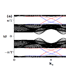
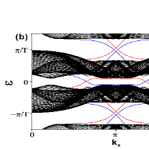
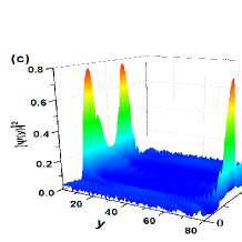
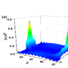
Figure 1: (color online) (a)(b) Spectrum of the truncated Floquet Hamiltonian (Eq.(6)) in the ZigZag geometry. The parameters used in (a) are $J=1$ (energy unit), $\lambda_{SO}=0.2$, $\lambda_{v}=1.2$, $J_{D}=1$, $\lambda_{SO,D}=0.1$, $\omega=3$. The parameters in (b) are the same as (a) except now $\omega=2$. (c) The density of the edge states traversing the gap at $\varepsilon=0$. (d) The density of the edge states traversing the gap at $\varepsilon=\pi/T$.

In Fig.1(a), the static parameters are chosen as $J=1$, $\lambda_{SO}=0.2$, $\lambda_{v}=1.2$. As $\lambda_{v}>3\sqrt{3}\lambda_{SO}$, the static model describes a trivial insulator C. L. Kane1 , then according to the bulk-edge correspondence, there is no edge state localized at the open boundary. With the introduction of periodically driving, we find when the driving frequency $\omega$ is much larger than other energy scales, there is a large energy gap between Floquet bands and no edge states traversing the gap. By decreasing the driving frequency, we find the gap at $\varepsilon=\pi/T$ will close and then reopen, with edge states emerging and traversing the reopened gap as shown in Fig.1(a), which suggests the Floquet band now is topologically nontrivial. The edge states are not chiral since each edge has states which propagate in both directions. As the Hamiltonian holds the time-reversal symmetry, the edge states are helical in the sense that fermionic atoms with opposite spin propagate in opposite direction, therefore, the system now is a driven QSH insulator. We name such driven QSH insulators as FQSH insulators. The helical edge states traversing the gap at $\varepsilon=\pi/T$ is a unique property of driven systems. For a static system, the helical edge states always appear in the gap at $\varepsilon=0$ because the spectrum of a static system is bounded M. S. Rudner .

For the sake of discussion, we introduce two $Z_{2}$ topological indices $\nu_{0}$ and $\nu_{\pi}$ to characterize the topological properties corresponding to the gap at $\varepsilon=0$ and $\varepsilon=\pi/T$, respectively. With this introduction, the trivial phase in the large driving frequency region is characterized by $(\nu_{0},\nu_{\pi})=(0,0)$ and the FQSH insulator exhibited in Fig.1(a) is characterized by $(\nu_{0},\nu_{\pi})=(0,1)$.

With a further decrease of the driving frequency, the gap at $\varepsilon=0$ will also close and then reopen. As a consequence, helical edge states traversing both gaps at $\varepsilon=\pi/T$ and $\varepsilon=0$, and therefore, there are two pairs of helical states propagating on the same boundary. Such “anomalous” edge states are without an analog in static system. In static QSH insulator, when there are even pairs of helical edge states, the edge states are no longer stable against disorder and one can always add some extra term to gap all of them, as a result, the system is topologically equivalent to a trivial insulator. However, for here the FQSH insulator characterized by $(\nu_{0},\nu_{\pi})=(1,1)$, the helical edge states traversing the gaps at $\varepsilon=\pi/T$ and $\varepsilon=0$ are separated by a big energy difference, as a result, their coupling effects can be neglected, and the two pairs of helical edge states are still stable against disorder. Fig.1(c)(d) show that these helical states are well localized at the two open boundaries of the system.

Periodic perturbation breaking the time-reversal symmetry— We add a periodic perturbation to the system,

$$V=V_{0}\sigma_{z}\cos(\omega t).$$ (8)

This perturbation breaks the time-reversal symmetry in the sense: $\mathcal{T}V\mathcal{T}^{-1}=-V$, with $\mathcal{T}=i\sigma_{y}\mathcal{K}$. Although the form of this perturbation is the same as the one in Ref.N. H. Lindner , the spaces on which the Pauli matrix $\sigma_{z}$ operates are different. In Ref.N. H. Lindner , $\sigma_{z}$ operates on the subspace of bands (similar to here the subspace of the two sublattices) in each $2\times 2$ block, and therefore, it does not break the whole system’s time-reversal symmetry. That’s the reason why a pair of helical edge states (a pair of chiral edge states in each $2\times 2$ block) can be driven up by the perturbation of this form. However, $\sigma_{z}$ here is a Pauli matrix purely operating on spin, consequently, it directly breaks the whole system’s time-reversal symmetry. For such a periodic perturbation, we find the original time-reversal symmetric static system can not be driven into a FQSH insulator but the perturbation also does not affect the edge states of a static QSH insulator and a FQSH insulator. The robustness of the FQSH insulator against the time-reversal-symmetry-breaking driving term implies that if there exist other driving terms which do not break the time-reversal symmetry, the system can be driven to be a FQSH insulator.

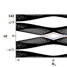
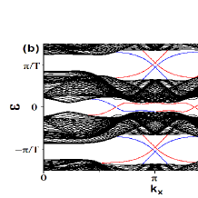
Figure 2: (color online) (a)(b) Spectrum of the truncated Floquet Hamiltonian (Eq.(6)) in the cylindrical geometry.The parameters used in (a) are: $J=1$, $\lambda_{SO}=0.2$, $\lambda_{v}=0.8$, $\omega=6.5$, $V_{0}=1$. As $\lambda_{v}<3\sqrt{3}\lambda_{SO}$, the static system is a QSH insulator, with helical edge states traversing the gap. The parameters in (b) are: $J=1$, $\lambda_{SO}=0.2$, $\lambda_{v}=1.2$, $J_{D}=1$, $\lambda_{SO,D}=0.1$, $\omega=2$, $V_{0}=1$.

For details, the static system with the parameters in Fig.2(a) is a QSH insulator, with helical edge states traversing the gap at $\varepsilon=0$. With the introduction of the time-reversal-symmetry-breaking perturbation, we find no edge states are driven up in the gap at $\varepsilon=\pi/T$, and the topology of the system is stable against the perturbation: the original helical edge states traversing the gap at $\varepsilon=0$ is almost unaffected by the perturbation. The robustness is due to that the meaning of “time-reversal-symmetry-breaking” here is quite different from the one for static system. In Ref.N. H. Lindner , the authors have discussed that even the Hamiltonian at any given time may not possess any symmetry under time reversal, the Floquet Hamiltonian possess the time-reversal symmetry as long as the condition $\mathcal{T}\hat{\mathcal{H}}(t)\mathcal{T}^{-1}=\hat{\mathcal{H}}(-t+\tau)$ holds (for some fixed $\tau$). That’s the reason why the helical edge states are not gapped out.

For a FQSH insulator, we find the condition can not be satisfied due to the existence of three driving terms (two terms from Eq.(3)), however, compared Fig.2(b) to Fig.1(b), it is direct to see that the helical edge states traversing both gaps are also robust against the perturbation. This may suggest that only the driven terms which do not hold the time-reversal symmetry is needed to satisfy the condition. This is reasonable, when the driven Hamiltonian only have driving terms which do not break the time-reversal symmetry, the Hamiltonian is time-reversal invariant at any time, consequently, the Floquet Hamiltonian is no doubt time-reversal invariant.

Theoretical model without time-reversal symmetry— To see whether such a driving approach can also drive a trivial system without time-reversal symmetry to be topological, we consider the familiar two-band tight-band model realized on a square lattice X. L. Qi ,

$$H_{0} = -\frac{J}{2}\sum_{i}[\psi_{i}^{{\dagger}}i\sigma_{x}\psi_{i+\hat{x}}+\psi_{i}^{{\dagger}}i\sigma_{y}\psi_{i+\hat{y}}+h.c.]$$ (9)

$$+ \frac{B}{2}\sum_{i}[\psi_{i}^{{\dagger}}\sigma_{z}\psi_{i+\hat{x}}+\psi_{i}^{{\dagger}}\sigma_{z}\psi_{i+\hat{y}}+h.c.]$$

$$+ M\sum_{i}\psi_{i}^{{\dagger}}\sigma_{z}\psi_{i}.$$

Here $\vec{\sigma}=(\sigma_{x},\sigma_{y},\sigma_{z})$ are Pauli matrices operating on spin, $J$ denotes the strength of spin-orbit coupling, $B$ and $M$ denote the difference between the two spin degrees’ hopping amplitude and on-site energy. Without loss of generality, we assume $B>0$ in this work.

Re-expressing the Hamiltonian under the representation $\psi_{\mathbf{k}}^{{\dagger}}=(c^{{\dagger}}_{\uparrow,\mathbf{k}},c^{{\dagger}}_{\downarrow,\mathbf{k}})$ in momentum space, we obtain

$$H_{0}=\sum_{\mathbf{k}}\psi_{\mathbf{k}}^{{\dagger}}\mathcal{H}_{0}(\mathbf{k})\psi_{\mathbf{k}},$$

with

$$\mathcal{H}_{0}(\mathbf{k}) = \vec{d}(\mathbf{k})\cdot\vec{\sigma}=J\sin(k_{x})\sigma_{x}+J\sin(k_{y})\sigma_{y}$$ (10)

$$+(M+B(\cos(k_{x})+\cos(k_{y})))\sigma_{z}.$$

This Hamiltonian is obviously without time-reversal symmetry, consequently, when $\vec{d}(\mathbf{k})$ does not vanish in the Brillouin zone, the topology of this static Hamiltonian is determined by the first Chern number D. Thouless ,

$$C_{1}=\frac{1}{4\pi}\int d^{2}\mathbf{k}(\frac{\partial\hat{d}(\mathbf{k})}{\partial k_{x}}\times\frac{\partial\hat{d}(\mathbf{k})}{\partial k_{y}})\cdot\hat{d}(\mathbf{k}),$$ (11)

where $\hat{d}(\mathbf{k})=\vec{d}(\mathbf{k})/|\vec{d}(\mathbf{k})|$, and the Chern number of this system is

$$C_{1}=\left\{\begin{array}[]{cc}1,&0<M<2B\\ -1,&-2B<M<0\\ 0,&\text{otherwise}.\end{array}\right.$$ (15)

By varying the optical lattice periodically, the parameters appearing in Eq.(9) will also vary with time periodically, $J_{x,y}(t)=J+J_{x,y}^{D}\cos(\omega t)$, $B_{x,y}(t)=B+B_{x,y}^{D}\cos(\omega t)$ and $M(t)=M+M_{D}\cos(\omega t)$. If we assume the two bands are close, $J_{x,y}^{D}$ can be much larger than $B_{x,y}^{D}$, $M_{D}$. Therefore, without loss of generality, we neglect $B_{x,y}^{D}$, $M_{D}$ for simplicity, then the time-dependent Hamiltonian is given as

$$\mathcal{H}(\mathbf{k},t)=\mathcal{H}_{0}(k)+\mathcal{H}_{D}(\mathbf{k})\cos(\omega t),$$ (16)

where $\mathcal{H}_{D}(\mathbf{k})=J_{x}^{D}\sin(k_{x})\sigma_{x}+J_{y}^{D}\sin(k_{y})\sigma_{y}$. The effect of varying the optical lattice potential is equivalent to varying the spin-orbit coupling periodically.

For the isotropic driving case, $J_{x}^{D}$ is equal to $J_{y}^{D}$. To see how the driving affects the topology of the system, we also consider the system with periodical boundary condition in $x$ direction and open boundary condition in $y$ direction.

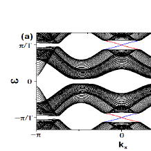
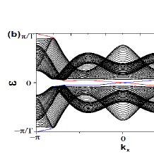
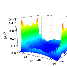
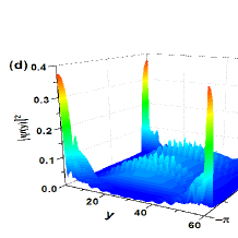
Figure 3: (color online) (a) (a) Floquet spectrum with parameters: $J$=1, $B=0.2$, $M=0.5$, $J^{D}_{x,y}=-0.5$, and $\omega=1.5$. (b) Floquet spectrum with parameters: $J=1$, $B=0.3$, $M=0.8$, $J^{D}_{x,y}=-0.5$, $\omega=1.3$. (c) The density of edge states corresponding to the gap at the quasienergy $\varepsilon=0$. (d) The density of edge states corresponding to the gap at the quasienergy $\varepsilon=\pi/T.$

Based on Eq.(15), the parameters in Fig.3(a) suggest the system in static is a trivial insulator without edge states. With the introduction of periodically driving, we find the picture is similar to the time-reversal symmetric case that when the driving frequency $\omega$ is much larger than other energy scales, there is a large energy gap between Floquet bands and no edge states. With decreasing the driving frequency, the gap at $\varepsilon=\pi/T$ firstly closes and then reopens, with edge states emerging and traversing the reopened gap as shown in Fig.3(a). As the system is without time-reversal symmetry, here the edge states are chiral in the sense that the fermionic atoms with opposite velocity propagate on the opposite boundary.

With a further decrease of the driving frequency, the gap at $\varepsilon=0$ will also close and then reopen. As a consequence, chiral edge states traverse both gaps at $\varepsilon=0$ and $\varepsilon=\pi/T$. As the winding number of a band is equal to the difference between the number of edge states at the gaps above and below the band, $C_{\varepsilon\varepsilon^{{}^{\prime}}}=n_{edge}(\varepsilon)-n_{edge}(\varepsilon^{{}^{\prime}})$, it is direct to see that the two bands’ winding numbers in Fig.3(c) are both zero. This is another unique property of a periodically driving system that the chiral edge states can exist despite the fact that the Chern numbers associated with both bands are zero M. S. Rudner . These chiral states are localized at the two open boundaries of the system, as shown in Fig.3(c)(d).

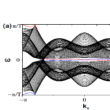
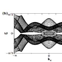
Figure 4: (color online) Anisotropic driving cases. (a) Driving along the $y$ direction, Floquet spectrum with parameters: $J$=1, $B=0.2$, $M=0.5$, $J^{D}_{x}=0$, $J^{D}_{y}=-0.5$, and $\omega=1.3$. (b) Driving along the $x$ direction, Floquet spectrum with parameters: $J=1$, $B=0.3$, $M=0.8$, $J^{D}_{x}=-0.5$, $J^{D}_{y}=0$ and $\omega=1.3$.

If we only drive the system along the $y$ direction, $i.e.$ $J_{D,x}=0$, $J_{D,y}\neq 0$, we find the results are similar to the isotropic case’s. Fig.4(a) shows that chiral edge states traverse both gaps, however, compared to the isotropic case under the same parameter condition except $J_{x}^{D}$, we find the gaps at $\varepsilon=0$ and $\varepsilon=\pi/T$ are greatly decreased. If we instead only drive the system in the $x$ direction, in other word, $J_{D,x}\neq 0$, $J_{D,y}=0$, the picture is dramatically changed. No matter what parameters are chosen, there is no edge state emerging, therefore, the system is always a trivial insulator, as shown in Fig.4(d). Although driving the system along the direction with periodical boundary condition will not induce chiral edge states at the open boundary, such a driving has the effect that it enlarges the energy gap.

Conclusions— We find that the optical lattice potential vary periodically provides a simple, general, and realizable way to drive a cold atomic system with or without time-reversal symmetry into phases with nontrivial topology. For a $\mathcal{T}$-invariant system, we find that this simple approach can drive the trivial insulator into a FQSH insulator but an external time-dependent field which couples with the spin and consequently breaks the time-reversal symmetry can not. The FQSH insulator, a novel state similar to the QSH insulator, can host one or two pair of helical edge states at the same boundary, and the edge states are robust against the time-reversal-symmetry-breaking periodic perturbation. Applying this driving approach to a system without time-reversal symmetry, we find that edge states driven up are chiral and the picture is similar to the one by driving the system with an external electromagnetic field.

Acknowledgments— This work was supported by NSFC Grant No.11275180 and National Science Fund for Fostering Talents in Basic Science No.J1103207.

References

- (1) C. L. Kane and E. J. Mele, Phys. Rev. Lett. 95, 146802 (2005).
- (2) C. L. Kane and E. J. Mele, Phys. Rev. Lett. 95, 226801 (2005).
- (3) B. A. Bernevig, T. L. Hughes, and S.-C. Zhang, Science 314, 1757 (2006).
- (4) M. König et al, Science 318, 766 (2007).
- (5) D. Hsieh et al, Nature 452, 970 (2008).
- (6) A. Y. Kitaev, Ann. Phys. (N.Y.) 303, 2 (2003).
- (7) A. P. Schnyder, S. Ryu, A. Furusaki, and A. W. W. Ludwig, Phys. Rev. B 78, 195125 (2008).
- (8) A. Y. Kitaev, AIP Conf. Proc. 1134, 22-30 (2009).
- (9) T. Kitagawa, M. S. Rudner, E. Berg, and E. Demler, Phys. Rev. A 82, 033429 (2010).
- (10) N. H. Lindner, G. Refael, and V. Galitski, Nat. Phys. 7, 490 (2011).
- (11) J.-I. Inoue and A. Tanaka, Phys. Rev. Lett. 105, 017401 (2010).
- (12) Z. Gu, H. A. Fertig, D. P. Arovas, and A. Auerbach, Phys. Rev. Lett. 107, 216601 (2011).
- (13) B. Dóra, J. Caysso, F. Simon, and R. Moessner, Phys. Rev. Lett. 108, 056602 (2012).
- (14) G. C. Liu, N. N. Hao, S. L. Zhu, and W. M. Liu, Phys. Rev. A 86, 013639.
- (15) Á. Gómez-León and G. Platero, Phys. Rev. Lett. 110, 200403 (2013).
- (16) N. H. Lindner, D. L. Bergman, G. Refae, and V. Galitski, Phys. Rev. B 87, 235131 (2013).
- (17) A. A. Reynoso and D. Frustaglia, Phys. Rev. B 87, 115420 (2013).
- (18) Y. T. Katan and D. Podolsky, Phys. Rev. Lett. 110, 016802 (2013).
- (19) D. E. Liu, A. Levchenko, and H. U. Baranger, Phys. Rev. Lett. 111, 047002 (2013).
- (20) A. Kundu and B. Seradjeh, Phys. Rev. Lett. 111, 136402 (2013).
- (21) M. Lababidi, I. I. Satija, and Erhai Zhao, Phys. Rev. Lett. 112, 026805 (2014).
- (22) P. M. Perez-Piskunow, G. Usaj, C. A. Balseiro, and L. E. F. Foa Torres, Phys. Rev. B 89, 121401(R) (2014).
- (23) A. G. Grushin, Á. Gómez-León, and T. Neupert, Phys. Rev. Lett. 112, 156801 (2014).
- (24) M. C. Rechtsman et al, Nature (London) 496, 196 (2013).
- (25) T. Kitagawa et al, Nat. Commun. 3, 882 (2012).
- (26) T. Kitagawa, E. Berg, M. Rudner, and E. Demler, Phys. Rev. B 82, 235114 (2010).
- (27) M. S. Rudner, N. H. Lindner, E. Berg, and M. Levin, Phys. Rev. X 3, 031005 (2013).
- (28) L. Jiang et al, Phys. Rev. Lett. 106, 220402 (2011).
- (29) L.-M. Duan, E. Demler, and M. D. Lukin, Phys. Rev. Lett. 91, 090402 (2003).
- (30) Z. Wang, X. L. Qi and S. C. Zhang, New. J. Phys. 12, 065007 (2010).
- (31) X. L. Qi, T. Hughes and S. C. Zhang, Phys. rev. B 78, 195424 (2008).
- (32) D. Thouless, M. Kohmoto, M. Nightingale, M. den Nijs, Phys. Rev. Lett. 49, 405, (1982)