Alkali vapor pressure modulation on the 100 ms scale in a single-cell vacuum system for cold atom experiments

Abstract

We describe and characterize a device for alkali vapor pressure modulation on the 100 ms timescale in a single-cell cold atom experiment. Its mechanism is based on optimized heat conduction between a current-modulated alkali dispenser and a heat sink at room temperature. We have studied both the short-term behavior during individual pulses and the long-term pressure evolution in the cell. The device combines fast trap loading and relatively long trap lifetime, enabling high repetition rates in a very simple setup. These features make it particularly suitable for portable atomic sensors.

I Introduction

Magneto-optical trap (MOT) loading is a limiting factor to the repetition rate of cold atom experiments. Fast loading is crucial for practical applications of cold atoms, such as atom interferometry Cronin, Schmiedmayer, and Pritchard (2009), as well as for experiments with high data volume, such as quantum state tomography of multiparticle entangled states Riedel et al. (2010); Haas et al. (2014). Ideally, the MOT loading time $t_{M}$ should be a small contribution to the cycle time, which means that it should be shorter than about 1 s in experiments involving evaporative cooling. The MOT loading rate $R$ is proportional to the partial vapor pressure of the element to be cooled (⁸⁷Rb in this article). Consequently, this pressure should be high for fast loading, but low for long lifetimes after loading. A widespread approach is to use a two-chamber vacuum system with differential pumping. However, this considerably increases the complexity of the vacuum and optical systems. An interesting alternative is to temporally modulate the vapor pressure inside a simple, single-cell apparatus. Light-induced atom desorption (LIAD) from the cell surfaces has been investigated for this purpose Anderson and Kasevich (2001); Hänsel et al. (2001); Atutov et al. (2003); Du et al. (2004); Klempt et al. (2006); Mimoun et al. (2010). Although it performs well in some experiments, there can be reproducibility issues, at least for Rb. The pressure modulation factor and also the effective capacity of the surfaces (i.e., the number of pulses before depletion) vary by orders of magnitude between experiments. Strong dependence on material properties such as surface contamination is a possible explanation Anderson (2012). Another, straightforward way to modulate the pressure of alkali vapors is to modulate the heating current in commercial alkali dispensers Wieman, Flowers, and Gilbert (1995). A fast pressure rise is easily achieved by using elevated heating currents. However, the timescale of pressure decay is typically between 3 and $4\,$s Wieman, Flowers, and Gilbert (1995); Fortagh et al. (1998); Rapol, Wasan, and Natarajan (2001); Fortágh et al. (2003); Bartalini et al. (2005); Scherer, Fenner, and Hensley (2012), too long to achieve a significant reduction of the cycle time. Here we show that this decay can be accelerated by more than an order of magnitude without sacrificing the simplicity and safe operation of a dispenser setup, by optimizing the thermal contact of the dispenser to an outside heatsink. Our device achieves pressure decay constants on the 100 ms timescale as desired, well within the range of interest for high repetition rate experiments.

The long-term pressure evolution in a pulsed-source system is influenced by slow processes such as adsorption-desorption dynamics, which can introduce timescales as long as several hours. Therefore, we also investigate the long-term evolution of ⁸⁷Rb pressure, background pressure and number of trapped atoms. As expected, the background pressure increases with the intensity of the dispenser pulses. We find evidence for both adsorption-desorption dynamics and slow heat-up of the vacuum apparatus. The latter effect is specific to our setup, which was not designed for this purpose, and we discuss straightforward improvements. In spite of these effects, we find that background pressure in our system remains lower than the pressure in a similar system with traditional, continuously heated dispenser, while the pulsed source accelerates MOT loading by more than an order of magnitude. This makes our system very attractive for many applications of cold alkali atoms.

The outline of this paper is as follows. We first discuss thermal coupling of the dispenser to the environment, motivate why an optimum range exists for this coupling, and estimate that the coupling found in usual experiments is too weak. Section III collects relevant facts about the mechanisms and time constants that govern the pressure evolution in the cell. In section IV, we describe our setup, where the thermal coupling is improved by copper parts which embrace the dispenser shell and thermally connect it to an outside heatsink. Sections V and VI present and discuss the experimental results obtained when this dispenser is used as a pulsed source for a MOT. It is shown that a steady-state regime can be established and its characteristics are investigated. Finally, section VII investigates the features of this steady-state regime as a function the alkali pulse intensity.

II Pressure modulation time constants and dispenser heat conduction

Alkali metal release from dispensers is a thermally activated process with a strongly nonlinear temperature dependence. Because of the high temperature involved, dispensers also release some “dirt”, such as water vapor Grüner et al. (2009). Cold atom experiments typically use commercial dispensers (SAES getters “FT-type” series) with constant heating currents between 3.5 and 4 A, corresponding to dispenser temperatures of about $500^{\circ}$C according to the manufacturer. To reach pressure modulation time constants in the 100 ms range, a first condition is that vapor release from the dispenser be modulated on this timescale, or faster. For our purposes, the dispenser must be brought to the desired temperature $T_{1}\sim 500^{\circ}$C in less than 100 ms, kept there for the MOT loading time, and then must cool down to significantly below $T_{1}$ in less than 100 ms. Fast heating is easily accomplished by applying a high-current pulse instead of continuous heating at lower current. The cooling timescale, however, is determined by the dispenser’s thermal coupling to the outside world.

We have measured $R=0.055\,\Omega$ for the resistance of the 12 mm long dispenser used in our experiments, so that the typical constant currents correspond to heating powers $P=0.7\ldots 0.9\,$W. In usual experiments, radiation and heat conduction through the connecting wires both contribute to the (inefficient) cooling of the dispenser. The following estimate gives an idea of the orders of magnitude. An upper limit of the dispenser’s heat capacity $C_{d}$ can be obtained from the easily measurable electrical heating power and heating time to reach alkali emission when heating rapidly from room temperature. Assuming that emission starts around $500^{\circ}\,$C, we obtain $C_{d}\leq 0.07\,\mbox{J}/\mbox{K}$ from our experimental data. (Some heat is lost to the mount during heating, which is why this method yields an upper limit only.) The power lost by radiation, $P_{\text{rad}}$, can be estimated from the dispenser surface. However, the result depends on the emissivity $\epsilon$ of the dispenser shell, which can be anywhere between $0.8$ and below $0.1$ for shiny metal. With $\epsilon=0.8$, one obtains $P_{\text{rad}}\approx 0.8\,W$ at $500^{\circ}$C for our dispenser size. The thermal conductance $h$ of the connecting wires is considerable – $h=5\,\mbox{mW}/\mbox{K}$ for a 1 mm diameter copper wire of 20 cm length – but is throttled by the mechanical connection between the dispenser and the wire. Given that $P<1\,$W, the effective $h$ must be $h\lesssim 2\,\mbox{mW}/\mbox{K}$, because otherwise the temperature of $500^{\circ}$C could not be reached.

To accelerate dispenser cooldown, the thermal conductance $h$ from the dispenser to the room-temperature reservoir must be significantly increased. The contribution from radiation loss can then be neglected, and we can model the temperature evolution with a simple heat equation:

$$C_{d}\dot{T}=P-h(T-T_{0})\,.$$ (1)

Here, $T_{0}$ is the reservoir temperature and we have taken the dispenser temperature to be homogeneous. For cooling ($P=0$) from an initial temperature $T(0)=T_{1}$, this equation leads to $T(t)=T_{0}+(T_{1}-T_{0})\exp(-t/\tau)$ with

$$\tau=\frac{C_{d}}{h}\,.$$ (2)

Improving the heat conduction $h$ has the desired effect of reducing $\tau$. However, we also need to consider the undesired heat flow from the dispenser to the reservoir during the heating phase, which increases with $h$. In our simple model, for heating with constant power and $T(0)=T_{0}$, the temperature rise is $T(t)=T_{0}+\frac{P}{h}(1-\exp(-t/\tau))$. The maximum temperature that can be obtained is

$$T(\infty)-T_{0}=\frac{P}{h}\,.$$ (3)

Therefore, as a first condition, $P$ must be large enough to maintain $P/h>T_{1}-T_{0}$. The heat flow to the reservoir during the heating phase is $\Phi_{l}(t)=P(1-\exp(-t/\tau))$ and the total energy leaking to the reservoir during heating to $T_{1}$ is $\frac{PC_{d}}{h}\ln(\frac{1}{1-(T_{1}-T_{0})h/P})-(T_{1}-T_{0})C_{d}$. It becomes neglegible for $P\gg h(T_{1}-T_{0})=\frac{C_{d}}{\tau}$. (This can also be seen by noting that $\Phi(t)$ remains small for $t\ll\tau$, and requiring that the heating time $t_{1}$ be $t_{1}\ll\tau$.) This shows that reservoir heating during dispensing can be kept small even for large $h$, by using a high heating power and a short heating time. Nevertheless, it would be wrong to conclude that $h$ should be made as large as possible. First, larger $h$ requires proportionally increased $P$, and $P$ is limited in practice. Moreover, an important practical limit comes from the fact that the required current exceeds the steady-state destruction threshold: when such a current is applied for too long, the dispenser melts like a fuse. The higher the current, the shorter the safety margin to destruction. With our holder described below, the required heating current is above 20 A. We have not made a systematic study of the destruction current, but we know from an unintentional experiment that a current of $40\,$A destroys the dispenser in less than 2 s. (A continuous current of 20 A is possible, though not desirable as it empties the dispenser in less than two days – another unintended experimental result.)

We conclude that an optimum regime exists for the thermal coupling $h$. It is situated between the usual, undercoupled, slow-cooling regime and an overcoupled regime with strong reservoir heating and/or high likelihood of dispenser overheating. Our dispenser mount brings $h$ into the optimum regime. Before proceeding, we note that the heat conduction model also provides an explanation for the slightly improved pressure decay in McDowall et al. (2012) and for the very fast decay observed in the laser-heated dispenser experiment Griffin, Weatherill, and Adams (2005) for low heating energies. In McDowall et al. (2012), the dispenser sleeves are attached to copper rods instead of wires, and the resulting pressure decay after dispenser turn-off has an initial decay constant of 1.8 s, about a factor of 2 faster than in experiments with wire-mounted dispensers Fortagh et al. (1998); Rapol, Wasan, and Natarajan (2001); Bartalini et al. (2005). In Griffin, Weatherill, and Adams (2005), the dispenser shell was attached to a ceramic plate over its full length, providing much higher $h$ than wire mounting. Additionally, only a fraction of the dispenser surface was laser heated so that the rest of the dispenser effectively acted as a well-coupled reservoir. The authors place an upper limit of 100 ms on the switch-off time. From the schematic shown in the article, it seems that the ceramic plate itself did not have a substantial thermal contact to the outside, which would provide an explanation for the much slower decay they observed for high heating powers. Another possibe explanation would be adsorption-desorption dynamics, treated below.

III Time constants of pumping and adsorption-desorption dynamics

Rapidly modulating the dispenser itself is not enough. Additionally, the timescale for evacuating excess alkali and dirt vapor after MOT loading must also be fast. If one considers the standard conductance formulas for the molecular flow regime, it seems easy to achieve a sufficiently fast pumping time constant, even with fairly small pumps. For our apparatus described below, the calculated pumping time constant (including tube lengths and angles) is 70 ms. However, these formulas describe an ideal gas and do not take into account the adsorption and desorption processes that occur for the highly reactive alkali vapor.

The binding energies and sticking times of alkali metals on UHV cell surfaces vary widely depending on the surface material and on the amount of coverage. It is difficult to obtain reliable data on the time constants and the situation appears to be particularly obscure for Rb, perhaps because its melting point is so close to room temperature. Nevertheless, some experimental facts are well established. First, there is the phenomenon sometimes called “curing”: when alkali vapor is first introduced from a reservoir into a freshly baked cell, it takes a long time, often several days, until a substantial vapor pressure can be created throughout the cell. This is most clearly observed in long UHV tubes or elongated cells Ma et al. (2009), but the phenomenon is general Wieman, Flowers, and Gilbert (1995) and we have observed it in all our experiments. Once a significant vapor pressure has been reached in the cell, it can then be adjusted on a much shorter timescale (tens of minutes) by adjusting the source rate, via a reservoir valve for example. The curing phenomenon suggests that clean surfaces form strong bounds with the impinging alkali atoms, whereas binding is much weaker once the surface has adsorbed a certain amount (often suggestively called a “monolayer”). The main consequence of the curing phenomenon in our context is that data should only be taken after the transitory curing phase has ended. All data presented below has been taken after several months of dispenser operation and fulfills this condition.

The cured surface still has a memory effect for its recent alkali exposure. It is well known, for example, that a small MOT can still be loaded for many hours after the source has been turned off. These timescales are too long to be explained by dispenser cool-down and suggest that some fraction of the alkali atoms stick to the cell walls and thus spend an average time $\tau_{s}$ (on the order of hours) inside the cell before being pumped away. To estimate the consequences of this effect, consider the following very crude model.

Two effects contribute to the alkali pressure in the cell $p(t)$. The dispenser releases atoms at a rate $r_{d}(t)$, and the cell walls can both release and capture atoms, changing the number of adsorbed atoms $N_{w}$:

$$p(t)=\alpha(r_{d}(t)-\dot{N}_{w})\,.$$ (4)

Here, $\alpha$ is a constant that depends on the pumping speed. $N_{w}$ is governed by a rate equation,

$$\dot{N_{w}}=-N_{w}\tau_{s}^{-1}+\beta r_{d}(t)\,,$$ (5)

where $\tau_{s}$ is the mean overall sticking time that an atom spends on the cell walls before being pumped out, and $0\geq\beta\geq 1$ is the total probability for an atom to stick to the cell walls rather than being pumped away directly. In an experiment with constant alkali release rate $r_{d}(t)=\bar{r}_{d}$ (“cw” experiment), $N_{w}$ will reach a steady state $N_{s}=\tau_{s}\beta\bar{r}_{d}$ which balances desorption and adsorption. Once this steady state has been reached, pressure no longer depends on the adsorption properties and remains constant at $p_{c}=\alpha\bar{r}_{d}$. In a pulsed experiment, the cycle time is typically less than a minute, while $\tau_{s}$ is expected to be much longer. Consequently, $N_{w}$ in the pulsed case will undergo only small oscillations about a steady-state value $N_{s}^{\prime}=\tau_{s}\beta\bar{r}_{d}^{\prime}$, where $\bar{r}_{d}^{\prime}$ is the release rate averaged over one cycle. For the purpose of this model, we will neglect the dispenser time constant and take $r_{d}^{\prime}(t)$ to be square pulses, with a constant high value during the MOT loading phase of duration $T_{M}^{\prime}$ and $r_{d}^{\prime}(t)=0$ during the “science” phase of duration $T_{s}^{\prime}$. The pressure during the science phase is then $p_{s}^{\prime}\approx\alpha N_{s}^{\prime}\tau_{s}^{-1}=\alpha\beta\bar{r}_{d}^{\prime}$.

Now we can compare a cw and a pulsed experiment which both use the same MOT setup (beam diameters, detunings, field gradients etc.) and load the same number $N$ of atoms into the MOT. For simplicity we assume that the alkali pressure dominates over other gases, so that the required release rate during MOT loading is inversely proportional to the MOT loading time (see IV.2 below for a discussion of MOT loading). In the cw case, this release rate is kept constant, so that $\bar{r}_{d}=\gamma T_{M}^{-1}$, where $\gamma$ is a constant depending on $N$ and on the MOT setup. The constant steady-state pressure is then

$$p_{c}=\alpha\gamma\frac{1}{T_{M}}\,.$$ (6)

For the pulsed case, a rate $\gamma{T_{M}^{\prime}}^{-1}$ is applied during the MOT loading phase, but the rate drops to zero during the science phase. The average rate is then $\bar{r}_{d}^{\prime}=\gamma/(T_{M}^{\prime}+T_{s}^{\prime})$ and the pressure during the science phase is

$$p_{s}^{\prime}=\alpha\gamma\frac{\beta}{T_{M}^{\prime}+T_{s}^{\prime}}\,.$$ (7)

The pressure during the science phase in the pulsed experiment is related to the constant pressure of the cw experiment by

$${p_{s}^{\prime}}=\beta\frac{T_{M}}{T_{M}^{\prime}+T_{s}^{\prime}}p_{c}\,.$$ (8)

The relation depends on the sticking probability $\beta$. Even for the worst case $\beta=1$, $p_{s}^{\prime}$ is lower than $p_{c}$ as long as the cycle time $T_{M}^{\prime}+T_{s}^{\prime}$ of the pulsed experiment is no shorter than the MOT loading time of the cw experiment. The ratio $T_{M}/(T_{M}^{\prime}+T_{s}^{\prime})$ reflects our assumption $\bar{r}_{d}\propto 1/T_{M}$ for a given $N$, which means that a constant fraction of the released atoms ends up in the MOT, independently of the rate $\bar{r}_{d}$ at which the MOT is loaded. If factors such as non-alkali background pressure change this relation, the ratio will change. Nevertheless, the qualitative trends predicted by eq. 8 should still be correct: In a pulsed experiment, for a given $N$, the pressure in the science phase increases for higher sticking probability and for shorter cycle time. Compared to a cw experiment with the same $N$, we expect that one can always achieve either a faster cycle or a reduced pressure in the science phase, even in a cell with unfavorable sticking properties. Achieving both improvements at the same time may also be possible, but requires the sticking probability to be significantly below 1.

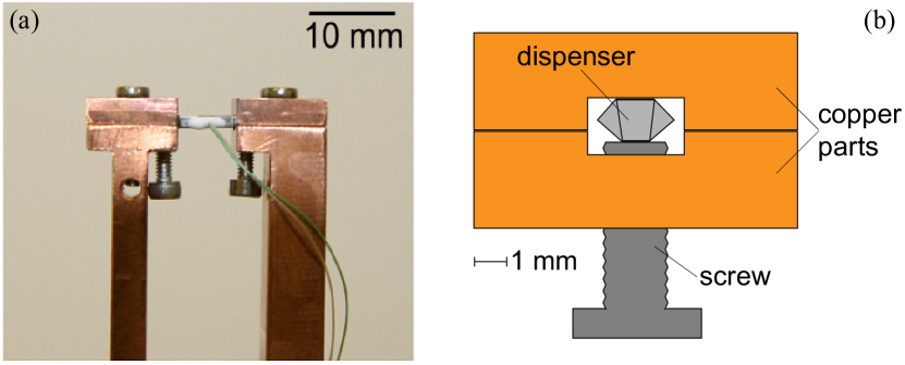
Figure 1: (a) Photo of the dispenser holder. Each of the two copper bars provides heat sinking from the dispenser and simultaneously serves as an electrical contact. (The thin wires and glue spot on the dispenser belong to a thermocouple that was used for thermal tests. They were not present on the devices used in the experiment.) (b) Schematic cross-sectional view of the copper clamp.

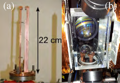
Figure 2: (a) Full view of the dispenser holder and copper flange. (Again, the thermocouple wires are not part of the final version.) The excessive length of the bars was necessary in our implementation because of the long glass-to-metal transition of our reused glass cell. (b) View of the glass cell containing the dispenser holder. The fluorescence collection lens is visible behind the cell.

IV Experiment

IV.1 Setup

In order to improve the heat flow out of the dispenser, we have mounted it in copper clamps on the top surface of massive copper bars, as shown in Figs. 1 and 2. The clamps provide a much better thermal contact than the spot-welded or crimped wires that are usually employed. The bars (cross section $\sim 1\,\mbox{cm}^{2}$) provide the thermal connection to a low-temperature reservoir outside the vacuum system. Ideally, they should be very short in order to keep their thermal resistance negligible. Our system is quite far from that ideal (Fig. 2) because we have reused an existing glass cell which had a particularly long glass-to-metal transition, so that the rods had to have a total length of 22 cm. This reduces the overall thermal conductivity and leads to a significant temperature rise in the upper part of the rods, contributing to the long-term behavior described below in sec. VI. In a purpose-built vacuum system, this length could be made much shorter. Heat-sinking from the copper bars is achieved by a copper flange that has the diameter of a standard CF copper gasket, but a thickness of several centimeters. The copper bars are screwed to the inside of this flange, while passive heatsinks or optionally water cooling can be attached to its outer surface. The quartz cell of volume 290 ml is pumped with a 25 l$/$s ion pump via a 35CF cross, tube (length 20 cm), and an angle valve. Taking into account the tubes and angles, the calculated pumping speed at the cell entrance is 4 l$/$s and the pumping time constant about 70 ms. The base pressure as indicated by the ion pump current is below $10^{-9}$ hPa.

The MOT is a standard setup with six independent beams. The axial gradient of the magnetic quadrupole field is 11 G$/$cm in all experiments reported here. In our test setup, the $1/e^{2}$ beam diameter (1.2 cm) and the power per beam (1.6 mW) are both small, which limits the trapped atom number. This should be taken into account when comparing our atom numbers to other experiments: atom numbers can be expected to increase by several orders of magnitude if the same dispenser assembly is used with the larger beam diameters and laser powers that are typical in state-of-the-art quantum gas experiments.

IV.2 Measurement methods

As mentioned above, all the experiments described here were carried out after several months of operation, i.e. long after the system had cured. Fluorescence light from the atoms in the beam intersection was collected by a 2 in diameter, $f=40\,$mm lens outside the glass cell, followed by an amplified photodiode. Unless otherwise indicated, the fluorescence was measured during MOT loading. Because of the uncertainties in solid angle and in the average dipole strength of the fluorescing atoms, the absolute values of our atom number and loading rate measurements are beset with a large systematic error.

To deduce the Rb pressure from the fluoresce during MOT loading, we use the well-established loading rate analysis (see for example Monroe et al. (1990); Mimoun et al. (2010); Arpornthip, Sackett, and Hughes (2012)). In our regime of moderately low trapped atom number $N$, MOT loading and decay are well described by

$$\dot{N}=R-\frac{N}{\tau_{\mathit{MOT}}}\,.$$ (9)

$R=\alpha_{R}p_{\text{Rb}}$ is the MOT loading rate, $p_{\text{Rb}}$ the partial pressure of ⁸⁷Rb and $\alpha_{R}$ is a constant that depends on the parameters of the MOT setup (beam diameter, detuning and intensity and magnetic field gradient). $\tau_{\mathit{MOT}}$ is the decay time constant due to collisions with the background gas. It is proportional to the sum of the partial pressures of ⁸⁷Rb and of all contaminants $i$ present in the vacuum chamber, each weighted with the relevant collisional cross section $\sigma_{\text{Rb-i}}$. We separate loss due to thermal Rb atoms from the loss that is independent of Rb pressure:

$$\tau_{\mathit{MOT}}^{-1}=\beta_{\text{Rb}}p_{\text{Rb}}+\tau_{b}^{-1}\,,$$ (10)

When pressures are constant, eq. 9 leads to

$$N(t)=N_{\text{f}}(1-e^{-\frac{t}{\tau_{\mathit{MOT}}}})$$ (11)

with

$$N_{\text{f}}=R\tau_{\mathit{MOT}}=\frac{\alpha_{R}p_{\text{Rb}}}{\beta_{\text{Rb}}p_{\text{Rb}}+\tau_{b}^{-1}}\,.$$ (12)

⁸⁷Rb pressure is proportional to $R$. The background pressure is roughly proportional to $\tau_{\mathit{MOT}}^{-1}$ because the collisional cross-sections of background gas constitutents are all comparable Arpornthip, Sackett, and Hughes (2012). Thus, both quantities can be deduced from $N(t)$. During the dispenser pulse, where pressures vary too fast for this solution to be valid, $R$ can still be measured from the initial linear rise in $N(t)$.

V Results: Pressure modulation

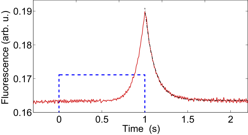
Figure 3: Pulsed dispenser emission observed in fluorescence, MOT coils switched off. A current of $I_{d}=20.2\,$A is applied for 1 s starting at $t=0$ (blue dashed curve). The red solid curve shows the fluorescence observed (signal averaged over 29 such pulses). This data was taken in steady state (i.e., after many identical pulse cycles). The decay time constant of the exponential fit (black dot-dashed line) is $\tau_{1}=112\,$ms.

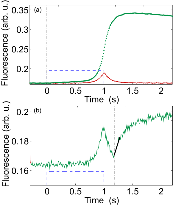
Figure 4: MOT fluorescence (green curves) during loading from the pulsed dispenser. Blue dashed curves indicate the timing of the current pulse (start at $t=0$, end at $t_{\text{end}}=1\,$s, $I_{d}=20.2\,$A). Black dashed lines show the start of the MOT loading (switching on the MOT coils), which occurs at $t=0$ in (a) and at $t=t_{\text{end}}+0.19\,$s in (b). The MOT signal in (a) is averaged over 10 shots, the signal in (b) is a single shot. The red curve in (a) recalls the time dependence of the rubidium vapor density in the cell (same data as in Fig. 3). The black solid line in (b) shows the initial slope of the MOT loading curve, which is used to deduce the pressure of ⁸⁷Rb in the cell at that time.

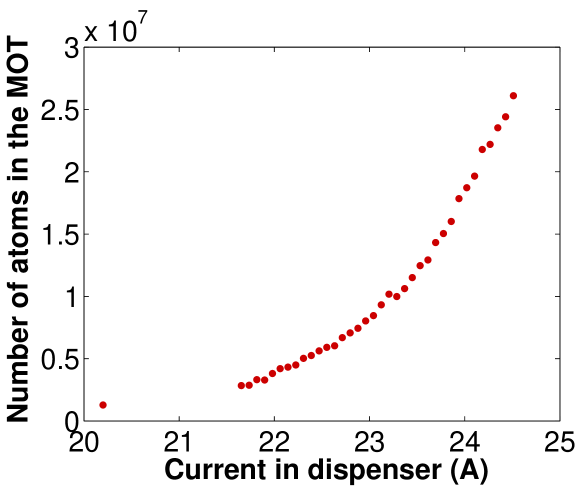
Figure 5: Number of atoms in the MOT as a function of dispenser current $I_{d}$. Current pulses had a duration of 1 s. MOT coils were switched on at the start of the current pulse and the atom number was measured 200 ms after the end of the pulse.

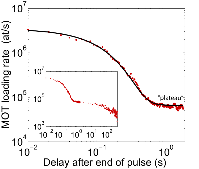
Figure 6: ⁸⁷Rb pressure as a function of the time $t_{0}$ after the end of a $1\,s$ dispenser pulse with $I_{d}=20.2\,$A. The initial loading rate of a MOT started at $t_{0}$ is used to measure the pressure. To be sure that steady-state conditions were reached, these measurements was taken after 10 hours of pulsed operation. The black solid line in the main graph is an exponential fit with offset as described in the text, which yields a decay time constant of 108 ms, in good a agreement with the fluorescence measurement above. Rb pressure decays by a factor of 51 during this fast decay. The inset shows data on a longer timescale, revealing a second, slower decay on the scale of 100 s.

In a first experiment, we measure ⁸⁷Rb fluorescence emanating from the beam intersection while applying short current pulses to the dispenser. The MOT magnetic field remains off. Therefore, the photodiode signal is proportional to the instantaneous pressure of room-temperature ⁸⁷Rb in the cell (with some integration due to a short-lifetime optical molasses created by the beams). Applying 1 s pulses with various currents $I_{d}$, we find that the threshold for ⁸⁷Rb emission lies around $I_{d}=18\,$A. Fig. 3 shows the fluorescence for $I_{d}=20.2\,$A. The rubidium pressure decay after the end of the pulse is well described by an exponential decay, yielding a time constant of $\tau_{f}=112\,$ms. This decay time is at least 20 times shorter than the values reported for bare dispensers Rapol, Wasan, and Natarajan (2001); Bartalini et al. (2005), confirming the validity of our approach. We have checked that the time constant depends only weakly on the value of $I_{d}$ and on the system temperature (see section VI below). We also observe that very little ⁸⁷Rb is emitted during the first $0.7\,s$: the dispenser heats up, but has not yet reached emission temperature. After this delay, the pressure rises very quickly to very high values. It would be possible to further accelerate the emission by using a higher current until emission starts and then lowering it, instead of the simple square pulses we use here.

Next, we have used these rubidium pulses to load the MOT. In Fig. 4(a), we use again $I_{d}=20.2\,$A and 1 s pulse duration, and the MOT coils are turned on together with the current pulse at $t=0$. Full loading takes about 1.2 s, including the 0.7 s heating time where no ⁸⁷Rb is emitted. As can be seen in the figure, most of the loading takes place during the final 0.5 s. It may be possible to further accelerate the cycle by starting the heating before the end of the preceding cycle. (We have not attempted to do this here.)

We have measured the number of trapped atoms as a function of dispenser current $I_{d}$. As before, current pulses were 1 s long and the MOT coils were turned on at the start of each pulse. Because the photodiode also receives fluorescence from untrapped background ⁸⁷Rb atoms (visible as a peak before MOT switch-on visible in fig. 4b), $N$ was measured 200 ms after the end of the pulse. (This time is long enough for background fluorescence to become small, while being shorter than MOT lifetimes at these pressures.) $N$ increases with $I_{d}$ and shows no saturation up to the highest currents that we dared to apply (Fig. 5). This suggests that the pressure of elements other than rubidium remains non-negligible even at the highest currents, but rises more slowly than $p_{\text{Rb}}$. The absolute numbers of $N\sim 2.5\cdot 10^{7}$ for the highest currents compare favorably to those of steady-state MOTs with similar beam diameters such as the TACC experiment in our lab Deutsch et al. (2010).

Measuring the initial linear slope of MOT loading curves provides an alternative and more sensitive way to measure $p_{\text{Rb}}$. We use a dispenser pulse duration of 1 s as before. We record fluorescence curves for various delays $t_{0}$ between the end of the current pulse and the start of MOT loading, which is initiated by switching on the coils. After each loading cycle, MOT coils are switched off for 0.3 s to purge all cold atoms. The measurements are analyzed by performing a linear fit to the fluorescence curve in a 100 ms time interval at the start of the MOT loading. Its slope yields the loading rate $R$ at $t_{0}$. To avoid measurement errors due to the background fluorescence mentioned above, we limit our analysis to times after the dispenser switch-off, where we have checked that the variation of background fluoresce is only a small contribution to the measured slope. (To obtain loading rates for earlier times, it would be possible to subtract the time-dependent background fluorescence, which can be measured independently by simply leaving the MOT coils off.) Fig. 4(b) shows an example fluorescence curve during one such cycle for $t_{0}=0.19\,$s. The curve $R(t_{0})$ resulting from many such measurements is shown in Fig. 6 on a log-log scale. To be sure that a steady state was reached, this measurement was taken after 10 hours of pulsed operation. As expected, the curve shows an evolution with two well-separated time scales. Pressure drops exponentially by a factor of 50 with a fast time constant of $\tau_{1}=108\,$ms. This time constant is in good agreement with the value obtained by the simple fluorescence measurement above. It then reaches a plateau, from which it decreases by at least another order of magnitude on a much slower time scale. Doubly exponential decay was observed in LIAD experiments Anderson and Kasevich (2001); Klempt et al. (2006). In our case, the slow decay is not well approximated by an exponential. Its timescale is roughly 200 s. We attribute it to a combination of cell heating and adsorption-desorption dynamics. (If the wall temperature was constant, it would allow us to estimate the sticking time $\tau_{s}$ of sec. III.) The long-term pressure evolution is studied in more detail in the next section.

To summarize these results, the rapid pressure drop by a factor of 50 in about $100\,$ms demonstrates the usefulness of this source for high-repetition-rate experiments. It confirms that dispenser cooldown was the limiting process for the slow pressure decay in previous pulsed-dispenser experiments, which used bare dispensers. In other words, in those experiments, source shut-off was much slower than the pumping processes. Although the pressure plateau reached after the fast decay is above the base pressure in the cell, the pressure modulation provides a significant advantage over the unmodulated dispenser. This becomes clear when comparing to a single-cell experiment with unmodulated dispenser, such as TACC Deutsch et al. (2010). TACC has somewhat larger MOT beam diameters (1.8 cm), a similar base pressure, and its constant Rb pressure is similar or higher than the pressure plateau observed here (loading rate $R\approx 3\times 10^{6}$at$/$s with $\tau_{\mathit{MOT}}=4.8\,$s). Yet, full MOT loading takes more than 10 s in TACC instead of 1.2 s here, and achieves an atom number that is at best comparable, and typically lower than observed here.

In the next section, we will try to get a better understanding of the plateau, and of the long-term evolution of the pressures in general.

VI Results: Long-term behavior

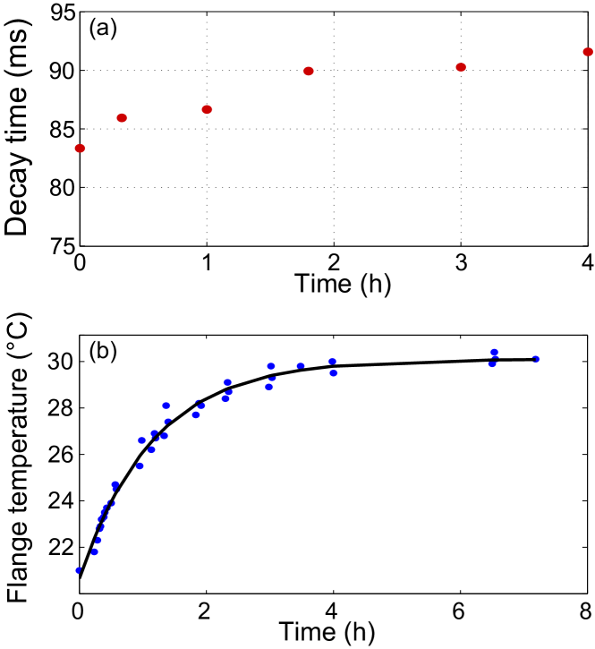
Figure 7: (a) Long-term evolution of the pressure decay time constant $\tau_{f}$. Current pulse with $I_{d}=21.2\,$A and 1 s duration were applied every 5 s. The decay time drifts by about 10% and settles after about two hours. (b) Temperature of the copper flange during a similar experiment. The time constant of the exponential fit (solid line) is 1.2 h, similar to the settling time in (a).

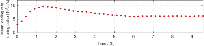
Figure 8: Long-term evolution of the mean MOT loading rate during the dispenser pulse. For $t<0$, the dispenser was permanently off for several hours (“cold start” at $t=0$). Starting from $t=0$, 1 s pulses with $I_{d}=24\,$A were applied every 5 s.

First, we examine the long-time stability of the pressure decay time constant $\tau_{f}$. As the Rb release from the dispenser is a very nonlinear function of temperature, $\tau_{f}$ might have a strong dependence on the temperature of the copper bars, which would be problematic because this temperature is difficult to control precisely. In this respect, our long copper bars represent a worst-case scenario: due to their length which limits heat evacuation, the temperature of the copper structure rises slowly during operation, and with it the mean dispenser temperature will rise as well. Therefore, we have repeated the decay time measurement of Fig. 3 every 5 s over a duration of 4 hours, using a current $I_{d}=21.2\,$A. Fig. 7(a) shows the result: the time constant undergoes an increase that is measurable, but remains below 10%. It occurs during the first 2 h; for longer times, $\tau_{f}$ remains constant within the error margin. We have also measured the evolution of the temperature at the base of the copper mount during a similar measurement (Fig. 7(b)). The temperature rises by about $9^{\circ}$C and settles with a time constant of about 1.2 h, comparable to the settling time of $\tau_{f}$. This suggests that the temperature change might indeed be responsible for the change in $\tau_{f}$. The steady-state value of 91 ms observed in this measurement is about 20% shorter than the one observed in Fig. 3 for $I_{d}=20.2\,$A. None of these variations will cause major perturbations for fast trap loading.

Another quantity of interest is the long-term evolution (over many pulses) of the peak ⁸⁷Rb pressure reached during the pulse. This determines the long-time evolution of the MOT loading rate and of the total number of trapped atoms per cycle. To measure it, we again apply a 1 s current pulse every 5 s over a long time (several hours to days). The MOT is switched on at the start of each pulse, and switched off for 300 ms before the next one to purge all cold atoms. We record the MOT fluorescence and deduce a mean loading rate during each pulse by dividing the total number of atoms measured 200 ms after the end of the current pulse by the useful pulse duration of 0.2 s (see Fig. 3). The result is shown in Fig. 8. The loading rate rises during the first 1.5 h. to a peak value which is about 1.7 times higher than the steady-state value. The steady state is reached after 5 to 6 h, which is rather long. This should not be a problem in practice: long time constants for pressure stabilization also appear when turning on a cw dispenser. Just as one keeps the cw dispenser switched on the whole day, the dispenser pulsing should be maintained the full day, even when the experiment is not being used for a while. Nevertheless, we would like to better understand this phenomenon, which is the subject of the next paragraphs.

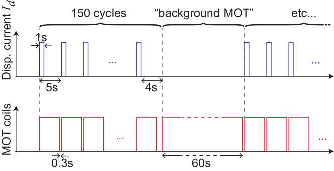
Figure 9: Timing sequence for measuring long-term evolution.

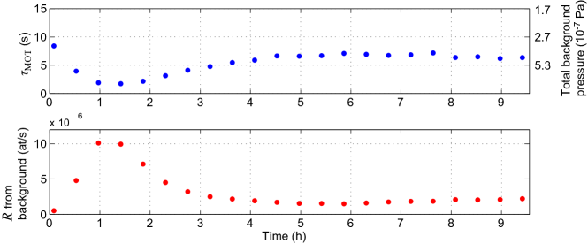
Figure 10: Long-term evolution of the low-pressure plateau. This data is obtained using the “Background MOT” (cf. Fig. 9). $\tau_{\mathit{MOT}}$ is a measure of the total pressure, while $R$ is proportional to the partial pressure of ⁸⁷Rb. The plateau pressures follow a pattern similar to the pulsed loading rate.

Two mechanisms introduce long time constants in our system. The first is caused by the slow heating due to excessive length of the copper bars, discussed and characterized above. The heating time constant is compatible with the pressure peaking time in Fig. 8. A mechanism that could cause the loading rate to peak and then decay in this scenario is release of previously adsorbed Rb from the copper surfaces. This effect will be substantially reduced in an improved mount with shorter copper bars.

The second, more fundamental effect is the adsorption-desorption dynamics of Rb on all internal surfaces of the cell. On the typical, cured surfaces, binding energies of Rb are much lower than on freshly cleaned ones. Hence, Rb atoms adsorbed to such a surface do not remain there forever, but are released after a time that can be on the scale of hours or days. Indeed, it is an empirical fact that Rb MOTs can still be loaded “from the background” hours and days after a cw dispenser has been switched off Wieman, Flowers, and Gilbert (1995). Moreover, the sticking probability and sticking time depend on the amount of Rb coverage already present on the surface.

Although it is not clear how the adsorption-desorption dynamics would explain the observed peak in the loading rate, these dynamics certainly play a role in the long-term evolution of the low-pressure plateau that is reached a few hundred ms after each dispenser pulse, and which will determine the lifetime of a magnetic or dipole trap with our source. To measure the plateau pressure, we insert measurements of MOT loading without dispenser pulse into our experiment cycle as shown in Fig. 9: after 150 of the normal 5 s cycles, we interrupt the repetitions, wait 4 s for the pressure to reach its plateau, and then record a MOT loading curve for a long time (60 s) with the source switched off (“background MOT”). After this, the next group of 150 normal cycles starts. The purpose of the background MOT is to obtain the plateau values of ⁸⁷Rb pressure and of the total pressure, and their long-term evolution. The loading curve of the background MOT is fitted with eq. 11 to extract the loading rate $R$ and the loading time $\tau_{\mathit{MOT}}$. $R$ is proportional to the ⁸⁷Rb partial pressure in the plateau, while $\tau_{\mathit{MOT}}$ can be used to estimate the total pressure using the conversion constant $2.7\times 10^{-6}\,\mbox{Pa s}$ established in Arpornthip, Sackett, and Hughes (2012).

Fig. 10 shows the long-term evolution of both quantities, measured over 9.5 h. The curves reveal that the pressures follow a pattern similar to the pulsed loading rate, with an extremum after 1…1.5 h and a steady state achieved after about 6 h. The plateau pressure of ⁸⁷Rb reached in the extremum is about a factor of 5 higher than the value reached in the steady-state. Total pressure and ⁸⁷Rb pressure show the same trends. This is not sufficient to establish the composition of the background gas, but at least suggests that the variations have a common origin. Once again, we expect this effect to be mitigated by using shorter copper rods.

VII Systematic study as a function of the loading rate

When the transient effects observed in the preceding section have ceased, the plateau pressure reaches a steady-state value, and this is the value that is most important to applications. Because of the mechanisms generating the plateau – wall adsorption and heating – the steady-state plateau pressure depends on the amount of ⁸⁷Rb released per pulse, and thus on the dispenser current $I_{d}$. Using again the measurement pattern of Fig. 9, we have measured the total and ⁸⁷Rb plateau pressures, as well as the loading rate during the pulse, for different values of $I_{d}$. For each $I_{d}$, measurements were performed over many hours to obtain the steady-state value. The results are shown in Fig. 11. As expected, both the loading rate during the pulse and the plateau pressures increase with the pulse intensity.

The figure also shows the product of atom number and lifetime, which is a figure of merit for evaporative cooling Anderson et al. (1994). This figure grows for loading rates up to $5\times 10^{7}$at$/$s and saturates for higher rates.

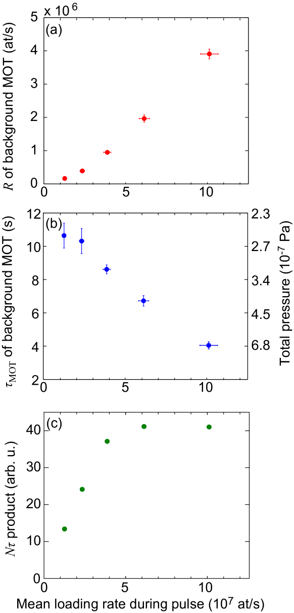
Figure 11: The currents of the pulses are $I_{d}=22.8\,\mbox{A},23.4\,\mbox{A},24.0\,\mbox{A},24.7\,\mbox{A},25.3\,\mbox{A}$.

Let us use Fig. 11 to compare again to a cw experiment. As above, we will compare to the TACC experiment ($R\approx 3\times 10^{6}$at$/$s, with $\tau_{\mathit{MOT}}=4.8\,$s and $N=1.4\times 10^{7}$, achieved after 10 s of loading). With the pulsed dispenser, using an intermediate loading rate of $5\times 10^{7}$at$/$s, the atom number is increased by more than a factor 2 and the lifetime by 1.5, while reducing the loading time by a factor of 10.

VIII Conclusion

The pulsed dispenser device demonstrated here provides alkali pressure modulation by more than an order of magnitude on the 100 ms timescale in both directions. While fast pressure rise with pulsed dispensers has been demonstrated before, the important new feature of our device is fast pressure decay after the pulse. Although the plateau pressure reached after this decay is above the base pressure, it is lower than the cw pressure in a similarly-sized nonpulsed MOT, while loading is at least an order of magnitude faster. This performance is achieved in a single-cell setup with only marginal added complexity over a standard MOT setup. These features make our device attractive for many applications of ultracold atoms, including single-cell Bose-Einstein condensation experiments with sub-second repetition rate and cold atom sensors for field use.

Several further improvements are possible. Our test setup had small beam $1/e^{2}$ beam diameters of 1.2 cm. Increasing this beam size would dramatically increase the number of trapped atoms Gibble and Chu. (1992) for the same alkali pressure, without any changes to the dispenser device itself. Using current pulses with an initial “boost” instead of square pulses would reduce the delay before alkali emission, further reducing the loading time. Total loading times below 300 ms are realistic with this improvement alone (cf. Fig. 3). As discussed in sec. IVA, shortening the copper holding bars should significantly reduce their temperature rise and the associated transient behavior. Furthermore, having shown that adsorption dynamics is an important factor for the plateau pressure, we expect that this pressure can be further reduced by improving the cell geometry and possibly by a suitable choice of cell materials. Our pulsed dispenser can also be combined with a nozzle such as described in McDowall et al. (2012) to direct atoms more efficiently towards the capture region. This may reduce the overall amount of alkali vapor released in every pulse. Finally, the pulsed dispenser can be combined with light-induced desorption (LIAD) to further increase the peak pressure and reduce the surface coverage during the low-pressure intervals. In a first test, we have observed a reduction of the ⁸⁷Rb pressure in the science phase by roughly $1/3$ when applying LIAD pulses simultaneously with dispenser pulses.