Approximate Stokes Drift Profiles in Deep Water

Abstract

A deep-water approximation to the Stokes drift velocity profile is explored as an alternative to the monochromatic profile. The alternative profile investigated relies on the same two quantities required for the monochromatic profile, viz the Stokes transport and the surface Stokes drift velocity. Comparisons with parametric spectra and profiles under wave spectra from the ERA-Interim reanalysis and buoy observations reveal much better agreement than the monochromatic profile even for complex sea states. That the profile gives a closer match and a more correct shear has implications for ocean circulation models since the Coriolis-Stokes force depends on the magnitude and direction of the Stokes drift profile and Langmuir turbulence parameterizations depend sensitively on the shear of the profile. The alternative profile comes at no added numerical cost compared to the monochromatic profile.

1 Introduction

With the inclusion of Langmuir turbulence (Skyllingstad and Denbo 1995, McWilliams et al. 1997, Thorpe 2004, Ardhuin and Jenkins 2006, Grant and Belcher 2009 and Belcher et al. 2012) and Coriolis-Stokes forcing (Hasselmann 1970, Weber 1983, Jenkins 1987, McWilliams and Restrepo 1999, Janssen et al. 2004, Polton et al. 2005 and Janssen 2012) in Eulerian ocean models it becomes important to model the magnitude and the shear of the Stokes drift velocity correctly. Stokes drift profiles are also needed when estimating the drift of partially or entirely submerged objects (see McWilliams and Sullivan 2000, Breivik et al. 2012, Röhrs et al. 2012 and references by Breivik et al. 2013a for applications of Stokes drift velocity estimates for particle and object drift). However, computing the Stokes drift profile is expensive since it involves evaluating an integral with the two-dimensional wave spectrum at every desired vertical level. It is also often impractical or impossible since the full two-dimensional (2-D) wave spectrum may not be available. For this reason it has been customary to replace the full Stokes drift velocity profile by a monochromatic profile matched to the transport and the surface Stokes velocity [see e.g. Skyllingstad and Denbo (1995), McWilliams and Sullivan (2000), Carniel et al. (2005), Polton et al. (2005), Saetra et al. (2007), Tamura et al. (2012)]. This is problematic, since it is clear that the shear under a broad spectrum is much stronger than that of a monochromatic wave of intermediate wavenumber due to the presence of short waves whose associated Stokes drift quickly vanishes with depth. At the same time, the deep Stokes drift profile will be stronger than that of a monochromatic wave since the low wavenumber components penetrate much deeper. It is therefore of interest to investigate profiles that exhibit stronger shear near the surface and a stronger deep drift. Here we explore an alternative approximate Stokes drift profile which will be compared to the monochromatic profile. The computation of the profile follows the same procedure as when estimating a monochromatic profile. The alternative profile has a lower mean-square error (MSE) than the monochromatic profile for all spectra tested, as will be shown in detail in later sections. It has a stronger shear in the upper part and does not tend to zero as rapidly as the monochromatic profile in the deeper part. This mimics the effect of a broader spectrum where the low wavenumber components penetrate deeper than the mean wavenumber component while the shorter waves (higher wavenumbers) only affect the the upper part of the water column. The proposed profile has the advantage of being robust, easy to implement and being computationally inexpensive. Importantly, it relies on the same two integrated parameters required to compute the monochromatic profile, namely the surface Stokes drift velocity and the Stokes transport. The proposed profile was recently implemented (see Janssen et al. 2013 and Breivik et al. 2013b) in the European Centre for Medium Range Weather Forecast’s (ECMWF) implementation of the NEMO ocean model [Madec and the NEMO team (2012); the coupled forecast system and the coupling between the wave model and the ocean model components are described by Janssen et al. (2013) and Mogensen et al. (2012)].

This paper is organized as follows. In Sec 2 we derive the analytical expression for the monochromatic Stokes drift profile and the alternative profile. In Sec 3 we investigate how these two approximate profiles compare for three well-known parametric spectra. Sec 4 examines the impact of a high-frequency spectral cut-off on the Stokes drift profile and the Stokes transport. This has implications for the computation of profiles from discretized spectra from numerical wave prediction models (Hasselmann et al., 1988; Tolman, 1991; Komen et al., 1994; Booij et al., 1999; Ris et al., 1999; Tolman et al., 2002; Janssen, 2004). We investigate how well the proposed profile fits the full profiles computed from two-dimensional wave spectra from the ERA-Interim reanalysis (Dee et al., 2011) in Sec 5. Here we also quantify how much waves beyond the high-frequency cut-off affect the shear and the magnitude of the Stokes drift profile (this was also investigated by Rascle et al. 2006). Furthermore, we investigate the impact of approximating the Stokes transport direction by the more readily available mean wave direction as well as approximating the magnitude of the Stokes transport vector by the first order moment. Sec 6 investigates profiles under observed wave spectra at Ekofisk in the North Sea. Finally, in Sec 7 we present our recommendations for the computation of approximate Stokes drift profiles.

2 Approximate Stokes Drift Profiles

The Stokes drift profile in water of arbitrary depth was shown by Kenyon (1969) to relate in the case of linear waves to the wave variance spectrum as

$$\mathbf{v}_{\mathrm{s}}(z)=g\int\!\int_{-\infty}^{\infty}F(\mathbf{k})\frac{\mathbf{k}}{\omega}\left[\frac{2k\cosh 2k(z+h)}{\sinh 2kh}\right]\,\mathrm{d}\mathbf{k},$$ (1)

where $k=|\mathbf{k}|$ is the magnitude of the wavenumber vector, $h$ is the bottom depth (positive), $g$ the gravitational acceleration, $\omega=2\pi f$ the circular frequency and $z$ is the vertical co-ordinate (positive up). To avoid confusion we use $v$ for Stokes drift velocities and $u$ for Eulerian currents. In the following we will only consider the deep-water limit of the dispersion relation,

$$\omega^{2}=gk.$$ (2)

Then Eq (1) simplifies to

$$\mathbf{v}_{\mathrm{s}}(z)=\frac{2}{g}\int\!\int_{-\infty}^{\infty}\omega^{3}\hat{\mathbf{k}}\mathrm{e}^{2kz}F(\mathbf{k})\,\mathrm{d}\mathbf{k},$$ (3)

where $\hat{\mathbf{k}}=\mathbf{k}/k$ is the unit vector in the direction of the wave component.

We now recast the east and north components of the Stokes drift profile in frequency-direction $(f,\theta)$ co-ordinates as

$$\mathbf{v}_{\mathrm{s}}(z)=\frac{16\pi^{3}}{g}\int_{0}^{2\pi}\!\int_{0}^{\infty}f^{3}\hat{\mathbf{k}}\mathrm{e}^{2kz}F(f,\theta)\,\mathrm{d}f\mathrm{d}\theta,$$ (4)

where $\theta$ is measured clockwise from north (going to). The Stokes transport $\mathbf{V}_{\mathrm{s}}=\int_{-\infty}^{0}\mathbf{v}_{\mathrm{s}}(z)\,\mathrm{d}z$ becomes in the deep-water limit

$$\mathbf{V}_{\mathrm{s}}=2\pi\int_{0}^{2\pi}\!\int_{0}^{\infty}f\hat{\mathbf{k}}F(f,\theta)\,\mathrm{d}f\mathrm{d}\theta.$$ (5)

The integrand here is the first-order moment of the wave spectrum, $m_{1}$, weighted by the unit vector $\hat{\mathbf{k}}$ of the wave component, with the $n$-th order moment of the 2-D spectrum defined as

$$m_{n}=\int_{0}^{2\pi}\!\int_{0}^{\infty}f^{n}F(f,\theta)\,\mathrm{d}f\mathrm{d}\theta.$$ (6)

Estimating the full profile from Eq (4) can be a costly operation even when a modeled or observed wave spectrum is available. When a wave spectrum is not available the Stokes drift profile must be approximated from the transport (5) and the surface Stokes drift velocity. It is therefore common to approximate Eq (4) by the exponential profile of a monochromatic wave [see eg Skyllingstad and Denbo (1995); McWilliams and Sullivan (2000); Carniel et al. (2005); Polton et al. (2005); Saetra et al. (2007); Tamura et al. (2012)]

$$v_{\mathrm{m}}=v_{0}\mathrm{e}^{2k_{\mathrm{m}}z}.$$ (7)

To ensure that the surface Stokes drift and the total transport of the monochromatic wave in Eq (7) agree with the values for the full spectrum, Eqs (4)-(5), the wavenumber must be determined by

$$k_{\mathrm{m}}=\frac{v_{0}}{2{V}_{\mathrm{s}}}.$$ (8)

A monochromatic profile will have a weaker vertical gradient than the profile under a full spectrum near the surface whereas it tends too quickly to zero deeper down. The behavior of the profile under a full spectrum is most readily investigated by considering the Phillips spectrum (Phillips, 1958, 1985; Janssen, 2004), applicable to the equilibrium range of the spectrum of wind-generated waves above the spectral peak,

$$F_{\mathrm{P}}=\left\{\begin{array}[]{lr}\alpha_{\mathrm{P}}g^{2}\omega^{-5},&\omega>\omega_{\mathrm{p}}\\ 0,&\omega\leq\omega_{\mathrm{p}}\end{array}\right.,$$ (9)

Here we set Phillips’ parameter $\alpha_{\mathrm{P}}=0.0083$ (there is some disagreement about its values with others workers, including Holthuijsen 2007 and Webb and Fox-Kemper 2011 preferring the value 0.0081). The peak circular frequency is denoted $\omega_{\mathrm{p}}$. The Stokes drift profile under (9) is

$$v_{\mathrm{P}}(z)=2\int_{\omega_{\mathrm{p}}}^{\infty}\alpha_{\mathrm{P}}g\omega^{-2}\mathrm{e}^{2\omega^{2}z/g}\,\mathrm{d}\omega.$$ (10)

which can be found analytically [see eg Gradshteyn and Ryzhik 2007, Eq (3.461.5)],

$$v_{\mathrm{P}}(z)=2\alpha_{\mathrm{P}}g\left[\frac{1}{\omega_{\mathrm{p}}}\exp{(2\omega_{\mathrm{p}}^{2}z/g)}-\sqrt{-2\pi z/g}\left(1-\mathrm{erf}(\omega_{\mathrm{p}}\sqrt{-2z/g})\right)\right].$$ (11)

The transport can also be found analytically,

$$V_{\mathrm{P}}=\frac{\alpha_{\mathrm{P}}g^{2}}{3\omega_{\mathrm{p}}^{3}}.$$ (12)

Near the surface ($|z|$ small), the term involving the error function becomes vanishingly small compared with the first term, and it is clear that

$$v_{\mathrm{P}}(z)\approx\frac{2\alpha_{\mathrm{P}}g}{\omega_{\mathrm{p}}}\mathrm{e}^{2k_{\mathrm{p}}z}.$$ (13)

Here we have introduced the peak wavenumber $k_{\mathrm{p}}=\omega_{\mathrm{p}}^{2}/g$. To investigate the behavior for large $|z|$ we substitute the following asymptotic expansion for the error function in Eq (11) [see Abramowitz and Stegun (1972), Eq (7.1.23)], valid for large $x$ (thus large $|z|$),

$$\mathrm{erf}(x)\approx 1-\frac{\mathrm{e}^{-x^{2}}}{x\sqrt{\pi}}\left(1-\frac{1}{2x^{2}}\right).$$ (14)

Hence, for large $|z|$ profile (10) drops off as

$$v_{\mathrm{P}}(z)\approx\alpha_{\mathrm{P}}g^{2}\frac{\mathrm{e}^{2k_{\mathrm{p}}z}}{2\omega_{\mathrm{p}}^{3}|z|}.$$ (15)

Motivated by this we have explored a profile which approaches the exponential shape (13) near the surface and which goes like the asymptotic solution (15) in the deep,

$$v_{\mathrm{e}}=v_{0}\frac{\mathrm{e}^{2k_{\mathrm{\mathrm{e}}}z}}{1-Ck_{\mathrm{\mathrm{e}}}z}.$$ (16)

The coefficient that was found to minimize the MSE for the Phillips spectrum over the entire profile is $C\approx 8$. Obviously the MSE takes into account discrepancies over the entire water column and will be more sensitive to deviations in the upper part where the drift is stronger. The transport under such a profile involves the exponential integral $E_{1}$ and can be solved analytically [Abramowitz and Stegun 1972, Eq (5.1.28)] to yield

$$V_{\mathrm{s}}=\frac{v_{0}\mathrm{e}^{1/4}E_{1}(1/4)}{8k_{\mathrm{e}}}.$$ (17)

It will in the following be referred to as the exponential integral profile. This imposes the following constraint on the inverse depth scale,

$$k_{\mathrm{e}}=\frac{v_{0}\mathrm{e}^{1/4}E_{1}(1/4)}{8V_{\mathrm{s}}}.$$ (18)

Here $\mathrm{e}^{1/4}E_{1}(1/4)\approx 1.34$, thus

$$k_{\mathrm{e}}\approx\frac{{v}_{0}}{5.97V_{\mathrm{s}}}\approx k_{\mathrm{m}}/3.$$ (19)

3 Profiles under Parametric Spectra

In the previous section we showed that the profile (16) approaches the profile under the Phillips spectrum (10) near the surface (13) and in the deep (15). We will now assess the quantitative and qualitative differences between the two approximate profiles, referred to by subscripts “m” for monochromatic and “e” for exponential integral, with respect to parametric spectra.

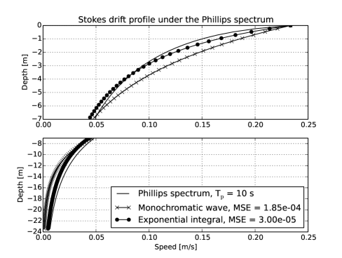
(b)

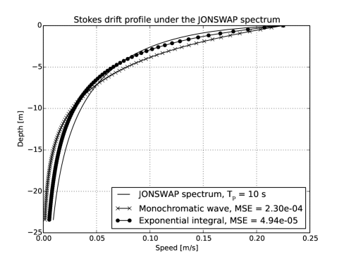
Figure 1: Panel a: The Stokes drift profile under the Phillips spectrum ($T_{\mathrm{p}}=10\,\mathrm{s}$). The upper part of Panel a is a zoom of the upper 7 meters for readability. The monochromatic approximation (x) tends to overestimate the drift in the upper part of the water column while underestimating the drift in the deeper part. The exponential integral approximation (o) exhibits closer correspondence throughout the water column, with an MSE about six times smaller than that found for the monochromatic approximation. Panel b: The Stokes drift profile under the JONSWAP spectrum ($T_{\mathrm{p}}=10\,\mathrm{s}$, fetch $X=10\,\mathrm{km}$). The results are similar to those for the Phillips spectrum with an MSE of the exponential integral (o) about 60% smaller than that of the monochromatic approximation (x).

The profile under the Phillips spectrum (10) is compared with the two approximate profiles (7) and (16) in Panel a of Fig 1. The exponential integral approximation has an MSE of about a sixth that of the monochromatic approximation. As mentioned in the previous section, the coefficient used for the fit is found by minimizing the MSE with respect to the Phillips spectrum. It is therefore not surprising that the match is good for this spectrum.

The Pierson-Moskowitz (P-M) spectrum (Pierson and Moskowitz, 1964) is commonly used to model fully developed (equilibrium) sea states,

$$F_{\mathrm{PM}}=\alpha_{\mathrm{P}}g^{2}\omega^{-5}\exp\left[-\frac{5}{4}\left(\frac{\omega_{\mathrm{p}}}{\omega}\right)^{4}\right].$$ (20)

We find the same general improvement as was found for the Phillips spectrum above with an MSE about a fifth that of the monochromatic approximation (not shown). Note that here the integral covers also the lower frequencies as the spectrum remains bounded for all frequencies. Panel b shows the profile under the JONSWAP spectrum. This spectrum is based on the P-M spectrum with a peak enhancement to account for the spectral shape found in fetch-limited seas (Hasselmann et al., 1973; Janssen, 2004; Webb and Fox-Kemper, 2011)

$$F_{\mathrm{JONSWAP}}=F_{\mathrm{PM}}\gamma^{\Gamma},$$ (21)

where

$$\Gamma=\exp\left[-\frac{1}{2}\left(\frac{f/f_{\mathrm{p}}-1}{\sigma}\right)^{2}\right].$$ (22)

Here typical values are $\gamma=3.3$, $\sigma=0.07$ for $f\leq f_{\mathrm{p}}$ and $\sigma=0.09$ when $f>f_{\mathrm{p}}$. The exponential integral profile gives a reduction in MSE of about 60% compared with the monochromatic profile (see Fig 1b).

3.1 The Shear of the Stokes Drift Profile

The production of Langmuir turbulence arises from a vortex force term, $\mathbf{v}_{\mathrm{s}}\times\nabla\times\mathbf{u}$, in the momentum equation (Leibovich, 1983). It is assumed that the vortex force gives rise to a term involving the shear of the Stokes drift velocity profile in the turbulence kinetic energy [Skyllingstad and Denbo (1995), McWilliams et al. (1997), Teixeira and Belcher (2002), Kantha and Clayson (2004), Ardhuin and Jenkins (2006), Polton and Belcher (2007), Grant and Belcher (2009) and Belcher et al. (2012)], although it is somewhat unclear whether this effect will be strong enough to explain the observed Langmuir circulation. The turbulent kinetic energy (TKE) equation with a Stokes drift shear term can be written

$$\frac{\mathrm{D}e}{\mathrm{D}t}=\frac{g}{\rho_{\mathrm{w}}}\overline{u^{\prime}_{3}\rho^{\prime}}-\overline{u^{\prime}_{i}u^{\prime}_{j}}\frac{\partial\overline{u}_{i}}{\partial x_{j}}-\overline{u^{\prime}_{i}u^{\prime}_{j}}\frac{\partial v_{i}}{\partial x_{j}}-\frac{\partial}{\partial x_{j}}(\overline{u^{\prime}_{j}e})-\frac{1}{\rho_{\mathrm{w}}}\frac{\partial}{\partial x_{i}}(\overline{u^{\prime}_{i}p^{\prime}})-\epsilon.$$ (23)

Here, $e\equiv q^{2}/2=\overline{u^{\prime}_{i}u^{\prime}_{i}}/2$ is the TKE per unit mass (with $q$ the turbulent velocity) and $\epsilon$ is the dissipation [see e.g. Stull (1988) p 152]. The term involving the Reynolds stresses multiplied by the gradient in Stokes drift velocity, $v_{i}$, represents production of Langmuir turbulence (McWilliams et al., 1997; Teixeira and Belcher, 2002; Ardhuin and Jenkins, 2006). By making the gradient transport closure approximation (Stull, 1988; Janssen, 2012), ignoring advective terms and horizontal gradients, and rewriting in vectorial form we arrive at

$$\frac{\partial e}{\partial t}=-\nu_{\mathrm{h}}N^{2}+\nu_{\mathrm{m}}S^{2}+\nu_{\mathrm{m}}\mathbf{S}\cdot\frac{\partial\mathbf{v}_{\mathrm{s}}}{\partial z}-\frac{\partial}{\partial z}(\overline{w^{\prime}e})-\frac{1}{\rho_{\mathrm{w}}}\frac{\partial}{\partial z}(\overline{w^{\prime}p^{\prime}})-\epsilon.$$ (24)

Here we have reverted to using $z$ for the vertical axis and $w$ for vertical velocities. We recognize in Eqs (23)–(24) the familiar terms of the TKE equation [see Stull 1988, Eq (5.1a)], namely shear production, $S^{2}=(\partial\overline{\mathbf{u}}/\partial z)^{2}$, and buoyancy production through the Brunt-Vaisälä frequency, $N^{2}=-(g/\rho)\mathrm{d}\rho/\mathrm{d}z$ ($\nu_{\mathrm{m,h}}$ are turbulent viscosity and diffusion coefficients, respectively) as well as the divergences of the pressure correlation term $\overline{w^{\prime}p^{\prime}}$ and turbulent transport $\overline{w^{\prime}e}$.

It is of interest to investigate the shear under parametric spectra, and for the Phillips spectrum (10) an analytical solution can be found [Gradshteyn and Ryzhik 2007, Eq (3.321.2)],

$$\frac{\partial v_{\mathrm{P}}}{\partial z}=2\alpha_{\mathrm{P}}g\int_{\omega_{\mathrm{p}}}^{\infty}\mathrm{e}^{-2\omega^{2}|z|/g}\,\mathrm{d}\omega=\sqrt{\frac{\pi g}{8|z|}}\mathrm{erfc}\left(\sqrt{\frac{2|z|}{g}\omega_{\mathrm{p}}}\right).$$ (25)

On the surface the shear goes to infinity. This is in contrast to the shear under a monochromatic wave (7), which remains bounded near the surface,

$$\frac{\partial v_{\mathrm{m}}(z=0)}{\partial z}=2k_{\mathrm{m}}v_{0}.$$ (26)

The shear of the exponential integral profile (16) also remains bounded, but reaches a value approximately 67% higher than the monochromatic profile at the surface,

$$\frac{\partial v_{\mathrm{e}}(z=0)}{\partial z}=10k_{\mathrm{e}}v_{0}\approx\frac{10}{3}k_{\mathrm{m}}v_{0}.$$ (27)

Technically the singularity in Eq (25) can be avoided by moving the computation of the Stokes shear away from the surface through the use of a staggered grid. It is also evident that for real ocean waves the spectrum will not extend to infinite wavenumbers (Elfouhaily et al., 1997). In practice, though, it may be necessary to cap the Stokes shear near the surface when estimating the Langmuir turbulence when assuming a tail proportional to $f^{-5}$ (see next Section).

4 High-frequency contribution to the profile

The same procedure as outlined in Sec 3 can be used to compute the profiles and transports from discretized wave spectra with a high-frequency cut-off. However, as the Stokes drift is weighted toward the high-frequency (HF) part of the spectrum, the tail beyond the cut-off frequency ($f_{\mathrm{c}}$) is significant both for the profile and the transport. We follow Komen et al. (1994) pp 233–234 and assume a tail of the form

$$F_{\mathrm{HF}}=F(f_{\mathrm{c}},\theta)\left(\frac{f_{\mathrm{c}}}{f}\right)^{5},$$ (28)

which is consistent with the Phillips spectrum (9). The two-dimensional spectrum below the cut-off frequency is here assumed to come from observations or from a numerical wave prediction model. This is the procedure used for adding the diagnostic high-frequency contribution to the spectrum in the WAM model, see Hasselmann et al. 1988; Komen et al. 1994; Janssen 2004 as well as the WaveWatch-III model, Tolman 1991; Tolman et al. 2002). In the ECMWF version of the WAM model (ECWAM, see ECMWF 2013 for further details), a lower diagnostic cut-off is set at

$$f_{\mathrm{d}}=\min(f_{\mathrm{max}},2.5\overline{f}_{\mathrm{windsea}}).$$ (29)

Here, $\overline{f}_{\mathrm{windsea}}$ is the mean frequency of windsea based on the first moment and $f_{\mathrm{max}}$ is the highest resolved frequency of the modeled spectrum. Above $f_{\mathrm{d}}$ the spectrum is treated diagnostically, ie, a tail of the form (28) overwrites the prognostic tail.

The high-frequency tail adds the following contribution,

$$\mathbf{v}_{\mathrm{HF}}(z)=\frac{16\pi^{3}}{g}f_{\mathrm{c}}^{5}\int_{0}^{2\pi}F(f_{\mathrm{c}},\theta)\hat{\mathbf{k}}\,\mathrm{d}\theta\int_{f_{\mathrm{c}}}^{\infty}\frac{\exp{(8\pi^{2}zf^{2}/g)}}{f^{2}}\,\mathrm{d}f.$$ (30)

The latter integral is similar to (10) and can be solved in a similar manner to (11) [see eg Gradshteyn and Ryzhik 2007, Eq (3.461.5)], yielding

$$\mathbf{v}_{\mathrm{HF}}(z)=\frac{16\pi^{3}}{g}f_{\mathrm{c}}^{5}\int_{0}^{2\pi}F(f_{\mathrm{c}},\theta)\hat{\mathbf{k}}\,\mathrm{d}\theta\left[\frac{\exp{(-\mu f_{\mathrm{c}}^{2})}}{f_{\mathrm{c}}}-\sqrt{\mu\pi}\left(1-\mathrm{erf}(f_{\mathrm{c}}\sqrt{\mu})\right)\right],$$ (31)

where $\mu=-8\pi^{2}z/g$. The high-frequency addition to the surface Stokes drift in deep water is

$$\mathbf{v}_{\mathrm{HF}}(0)=\frac{16\pi^{3}}{g}f_{\mathrm{c}}^{4}\int_{0}^{2\pi}F(f_{\mathrm{c}},\theta)\hat{\mathbf{k}}\,\mathrm{d}\theta.$$ (32)

ECWAM (ECMWF, 2013) computes and outputs the surface Stokes drift velocity vector corrected for the high-frequency contribution. The tail contribution to the transport is

$$\mathbf{V}_{\mathrm{HF}}=\frac{2\pi}{3}f_{\mathrm{c}}^{2}\int_{0}^{2\pi}F(f_{\mathrm{c}},\theta)\hat{\mathbf{k}}\,\mathrm{d}\theta.$$ (33)

5 Modeled Profiles in the North Atlantic

The ERA-Interim is a continuously updated atmospheric and wave field reanalysis produced by ECMWF, starting in 1979. The model and data assimilation scheme of the reanalysis are based on Cycle 31r2 of the Integrated Forecast System (IFS). ECWAM is coupled to the atmospheric part of the IFS (see Janssen 2004 for details of the coupling and Dee et al. 2011 for an overview of the ERA-Interim reanalysis). The resolution of the wave model component is $1.0^{\circ}$ on the Equator but the resolution is kept approximately constant globally through the use of a quasi-regular latitude-longitude grid where grid points are progressively removed toward the poles (Janssen, 2004). A similar scheme applies for the atmospheric component, but here the resolution is approximately $0.75^{\circ}$ at the Equator. The wave model is run with shallow water physics where appropriate. The spectral range from $3.45\times 10^{-2}$ to $0.55\,\mathrm{Hz}$ is spanned with 30 logarithmically spaced frequency bands. The angular resolution is $15^{\circ}$.

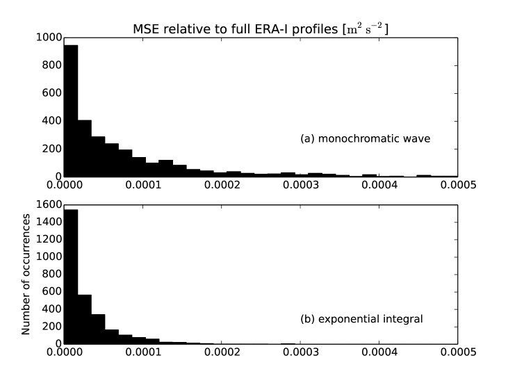
Figure 3: Panel a: The MSE between the full Stokes profile and the monochromatic profile to 30 m depth (vertical resolution 0.1 m). Panel b: The MSE of the exponential integral profile is on average about one third that of the monochromatic profile shown in Panel a.

For this study we computed the Stokes drift profiles down to 30 m depth from the two-dimensional ERA-Interim spectra in a region in the north Atlantic ocean ($59-60^{\circ}$N, $20-19^{\circ}$W, see Fig 2) for the whole of 2010. This region is stormy while also exposed to swell, providing a range of complex wave spectra. To assess the difference between the monochromatic approximation and the exponential integral approximation the MSE from the full Stokes drift profile to 30 m depth was calculated for every spectrum. The results are shown in Fig 3.

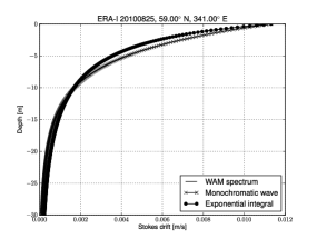
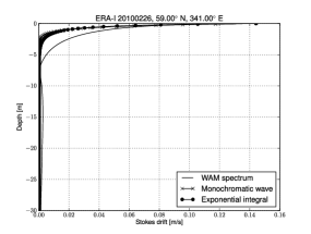
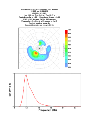
(a)	(b)

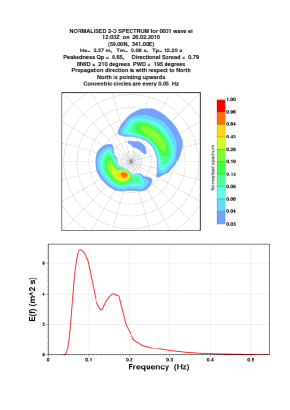
Figure 4: Panel a: The Stokes drift profile under a full two-dimensional wave spectrum from the ERA-Interim reanalysis. The location is in the north Atlantic. An extremely good fit is found in this case. The 2-D spectrum shows a strong bimodality which is masked in the 1-D spectrum. Panel b: Much poorer fit is found in this case where a strong swell system is superimposed on locally generated wind sea. There is still some improvement over the monochromatic approximation. Here the swell part is dominant and of a lower frequency, making the 1-D spectrum bimodal.

The MSE of the exponential integral profile from the full Stokes profile is on average 35% that of the monochromatic profile for our chosen location and model period (2010). The improvement is consistent for a range of different sea states, as illustrated in Fig 4. In Panel a the match is so close that the exponential integral profile overlaps the full profile. Poor performance is expected in cases where a one-dimensional fit is made to wave spectra with two diametrically opposite wave systems. Such a case is shown in Panel b, where a swell system travels in the opposite direction of the wind sea. Indeed, this spectrum represents the worst fit found throughout the model period, but even here there is slight improvement over the monochromatic approximation.

5.1 Tail-sensitivity of Modeled Stokes Drift Profiles

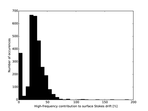
(b)

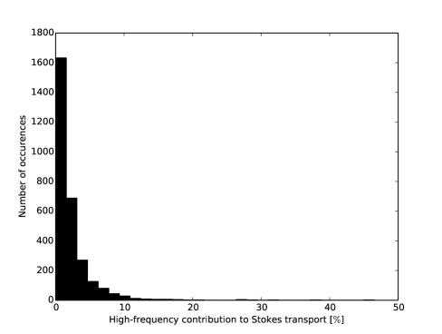
Figure 5: Panel a: Ratio of high-frequency contribution to the surface Stokes drift. On average the contribution is about 39%. Panel b: Ratio of high-frequency contribution to the Stokes transport. On average the contribution is about 3%, and only occasionally will it exceed 10%.

It is well known that adding the contribution from the high-frequency tail is important, and indeed it is standard practice to include it in the computation of the surface Stokes drift velocity (see eg the ECMWF model documentation, ECMWF 2013, p 52). We find that the contribution from the spectral tail to the surface Stokes drift velocity found in Eq (31) on average is about a third, and sometimes exceeding 75% (Fig 5, Panel a). In contrast, its contribution to the transport (33) is generally small (average 3%, Panel b, Fig 5), although in certain cases it may exceed 10%.

The high-frequency contribution decays rapidly with depth, as can be seen in Panel a of Fig 6. Below 0.5 m the difference between the low-frequency (LF) profile and the full profile is negligible. Neither of the approximate profiles is a particularly good match, but of the two the exponential integral profile has a slightly better gradient than the monochromatic profile. This mismatch in the upper half meter is in contrast to the good overall match found for the whole water column (see Fig 4). Panel b shows the approximate profiles instead pegged to the low-frequency surface Stokes drift with the high-frequency contribution added after. Now the gradient is much closer to that of the theoretical full Stokes profile, with the exponential integral profile being a good match. In principle it is straightforward to add this contribution to the approximate profile by way of Eq (31), but it requires knowledge of the two-dimensional wave spectrum at the cut-off frequency $f_{\mathrm{c}}$.

These results are to some extent dependent on the way the tail is formulated [see Eqs (28)-(29) and ECMWF (2013), p 52]. Ardhuin et al. (2009) argues that the high-frequency fit to buoy data is better when using a revised dissipation source function rather than the formulation presented by Bidlot et al. (2007) which is currently employed by ECWAM. However, the analytical form of the approximate profile has been shown to fit analytical and empirical spectra well (cf Sec 3), and it seems unlikely that a revised dissipation will seriously change the results found here.

5.2 Discrepancy Between the Stokes Transport and $m_{1}$

It is clear that

$$|\mathbf{V}_{\mathrm{s}}|\leq 2\pi m_{1},$$ (34)

but it is not clear how large this deviation is on average for typical wave spectra in the open ocean. Assessing the overestimation is of practical value since the first spectral moment is often archived or indirectly measured. Since the mean frequency is defined as $\overline{f}=m_{1}/m_{0}$ (World Meteorological Organization, 1998; Holthuijsen, 2007) and the significant wave height $H_{m_{0}}=4\sqrt{m_{0}}$, we can derive the first moment from the integrated parameters of a wave model or from wave observations and find an estimate for the Stokes transport,

$$\mathbf{V}_{\mathrm{s}}\approx\frac{2\pi}{16}\overline{f}H_{m_{0}}^{2}\hat{\mathbf{k}}_{\mathrm{s}}.$$ (35)

Here $\hat{\mathbf{k}}_{\mathrm{s}}=(\sin\theta_{\mathrm{s}},\cos\theta_{\mathrm{s}})$ is the unit vector in the direction $\theta_{\mathrm{s}}$ of the Stokes transport.

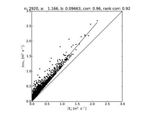
(b)

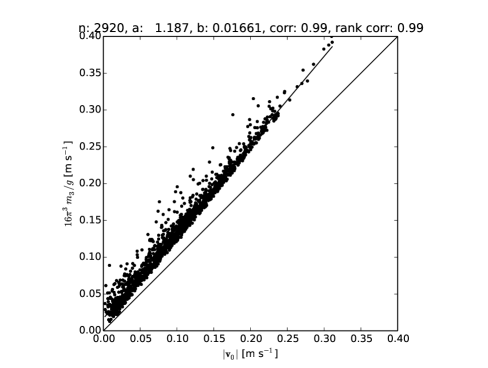
Figure 7: Panel a: The discrepancy between the two-dimensional Stokes transport $|\mathbf{V}_{\mathrm{s}}|$ and the unidirectional estimate $2\pi m_{1}$ from the ERA-Interim reanalysis. Good agreement is generally found, but the unidirectional estimate will on average be 16% too high. Panel b: The discrepancy between the two-dimensional surface Stokes drift $|\mathbf{v}_{0}|$ and the unidirectional estimate $16\pi^{3}m_{3}/g$. The unidirectional estimate will on average be 18% too high.

Note that this Stokes transport direction is not normally archived by wave prediction models (an exception being the more than 20-year long hindcast data set presented by Rascle and Ardhuin 2013), but it can be approximated by the mean wave direction $\overline{\theta}$ as will be shown later. Estimating the Stokes transport from the first moment is attractive since it involves only integrated parameters readily available from wave models. Fig 7a shows good correspondence between the the Stokes transport and the estimate based on $m_{1}$ in Eq (35) with a correlation coefficient of $0.96$, but $m_{1}$ will overestimate the transport on average by $17\%$. Both transport estimates include the contribution from the diagnostic high-frequency spectral tail. Similarly, the surface Stokes drift velocity

$$|\mathbf{v}_{0}|\leq 16\pi^{3}m_{3}/g.$$ (36)

The estimate from $m_{3}$ will on average be about $19\%$ too high (Fig 7b). This is very close to the number reported by Ardhuin et al. (2009) in their Appendix C (a reduction factor of 0.84).

5.3 Deviation between the Stokes transport direction and the mean wave direction

The mean wave direction (MWD) measured clockwise from north in the direction the waves are propagating to is defined as

$$\overline{\theta}=\mathrm{arctan}\left(\frac{\int_{0}^{2\pi}\!\int_{0}^{\infty}\sin\theta F(f,\theta)\,\mathrm{d}f\mathrm{d}\theta}{\int_{0}^{2\pi}\!\int_{0}^{\infty}\cos\theta F(f,\theta)\,\mathrm{d}f\mathrm{d}\theta}\right).$$ (37)

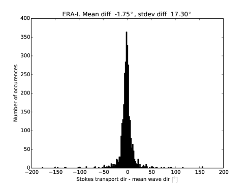
(b)

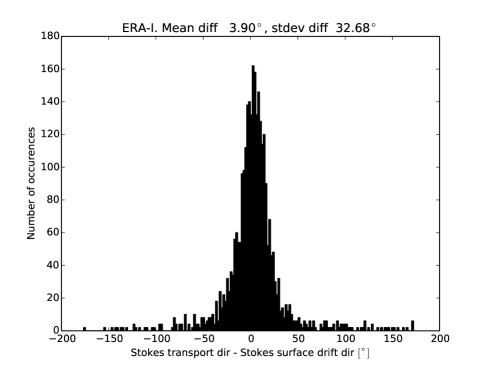
Figure 8: Panel a: The directional deviation between the Stokes transport and the mean wave direction (MWD). The average deviation is about $2^{\circ}$ and 75% of the time the difference is less than $10^{\circ}$. Panel b: The directional deviation between the Stokes transport and the surface Stokes drift velocity is larger due to the $f^{3}$ weighting of the wave spectrum which gives larger weight to high-frequency wave components.

It is of interest to assess how well it approximates the direction of the Stokes transport since it is a standard output parameter of many wave models (ECMWF, 2013) whereas the Stokes transport is generally not. Panel a of Fig 8 shows the deviation of the Stokes transport from the MWD in the model location in the north Atlantic during 2010. The average deviation is about $2^{\circ}$ and 75% of the time the difference is less than $10^{\circ}$. In contrast, Panel b shows a much larger deviation between the direction of the Stokes transport and the surface Stokes drift velocity. This is due to the sensitivity to high-frequency wave components arising from the third power of the frequency $f$ under the integral in Eq (4). It will therefore in general be better to estimate the transport direction from the mean wave direction rather than from the surface Stokes direction.

6 Stokes Profiles under Measured Spectra in the North Sea

A directional Datawell Waverider buoy anchored near Ekofisk in the central North Sea (56.5^∘N, 003.2^∘E) provided one year of data (2012) at 2 Hz sampling rate (location marked with asterisk in Fig 2b). 24,894 spectra from 20-min time series were computed, with some gaps (about 5% of the time series were either missing or discarded). The 2,400 measurements in the 20-min time series were split into 8 non-overlapping parts and a Hann window [Press et al. (2007) pp 656–660 and Christensen et al. (2013)] was applied to each chunk,

$$w_{n}=\frac{1}{2}\left(1-\cos\frac{\pi n}{N}\right).$$ (38)

Here the taper width $N$ was set to 32. Finally, the power spectrum was smoothed with a triangular filter

$$\overline{F}_{j}=(F_{j-1}+2F_{j}+F_{j+1})/4.$$ (39)

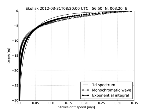
(b)

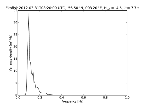
Figure 9: Panel a: The Stokes drift profile under the one-dimensional spectrum at Ekofisk in the central North Sea. A better fit is found with the exponential integral profile even in the presence of high-frequency spectral noise. Panel b: The spectrum was computed from a 20-min 2 Hz time series from a Datawell Waverider buoy. The spectrum is plotted up to the Nyquist frequency at 1 Hz. High-frequency noise affects the surface Stokes drift estimates somewhat.

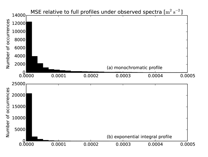
Figure 10: Panel a: The MSE between the full Stokes profile computed under a 20-min 2 Hz time series from a Datawell Waverider buoy at Ekofisk and the monochromatic profile to 30 m depth (vertical resolution 0.1 m). Panel b: The MSE of the exponential integral profile is on average about 40% that of the monochromatic profile shown in Panel a.

The results are very similar to what is found for the modeled spectra (Fig 9), with an MSE for the exponential integral profile 60% lower than for the monochromatic profile (cf Fig 10). The high-frequency part of the observed spectra tends to be rather noisy. This affects the surface Stokes drift and makes it sensitive to the high-frequency tail contribution (30)-(31), clearly illustrated by the spectrum shown in Fig 9b. Nevertheless, the match is better both with an without the added tail (about 50% reduction in MSE with tail added, not shown). Although the water depth at Ekofisk is only 70 m, the deep water approximation will hold in most cases and shallow water effects for the highest storm situations are not likely to affect the results significantly.

7 Recommendations for Approximate Stokes Drift Profiles

The alternative profile proposed here has been shown to be a better approximation than the monochromatic approximation for both theoretical spectra, modeled 2-D spectra in the open ocean and 1-D observed spectra. Utilizing this alternative profile comes at no added cost since the computation relies on the same two parameters required for the monochromatic profile, namely the Stokes transport, $\mathbf{V}_{\mathrm{s}}$, and the surface Stokes drift velocity, $\mathbf{v}_{0}$. We also found that in the open ocean the mean wave direction serves as a good proxy for the Stokes transport direction. It is a significantly better substitute than the surface Stokes drift direction. Furthermore, the one-dimensional first order moment, $m_{1}$, is found to correlate well with the magnitude of the two-dimensional transport, $|\mathbf{V}_{\mathrm{s}}|$. A reduction factor of 0.86 is appropriate in open ocean conditions.

Discretized spectra add a diagnostic high-frequency tail, see Eq (28). We find that adding the contribution from the tail gives an important contribution to the Stokes drift velocity in the upper half meter in the open ocean. Its impact rapidly decays, and below 0.5 m the difference is marginal (Panel a, Fig 6). This has implications for the computation of the gradient of the Stokes drift in the uppermost part of the ocean. Neither of the approximate profiles match the gradient in the upper half meter well, and this is important to keep in mind for future studies of upper-ocean turbulence. We note again that although it is numerically inexpensive to treat the high-frequency contribution to the profile separately, unless it has been explicitly archived, its reliance on the full 2-D spectrum makes this approach impractical for many applications where the spectrum is not available.

We conclude that the proposed Stokes drift profile is a much closer match than the commonly used monochromatic profile both in terms of speed and shear. Although neither profile is a good match for the shear in the upper half meter, even here the new profile offers a slight improvement over the monochromatic profile. As Langmuir turbulence depends sensitively on the Stokes drift shear the question of whether approximate profiles can be found that more closely mimic the gradient in the uppermost half meter merits further work.

(a)

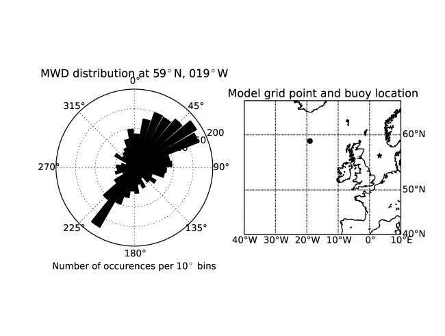
Figure 2: Left panel: The directional distribution of the mean wave direction (going to) in model location 59^∘ N, 019^∘ W. A large spread in wave direction is found. The location has a high prevalence of wind sea but is also exposed to swell. Right panel: Model location (circle) and buoy location (*) at 56.5^∘N, 003.2^∘E.

(a)

(a)

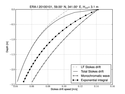
(b)

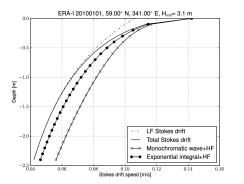
Figure 6: Panel a: The high-frequency contribution to the Stokes drift velocity. The Short waves beyond the cut-off frequency contribute only to the drift in the upper half meter (compare the dash-dotted low-frequency Stokes drift to the total drift drawn with a full line). The two approximate profiles are pegged to the surface Stokes drift and coincide exactly at the surface. The shear is not well represented by either of the approximate profiles in the upper half meter, but the exponential integral profile is the better match of the two. Panel b: The same approximate profiles with the high-frequency profile added. A much better match for the upper meters of the ocean is achieved, both in terms of shear and absolute error.

(a)

(a)

(a)

References

- Abramowitz and Stegun (1972) Abramowitz, M., Stegun, I. A. (Eds.), 1972. Handbook of Mathematical Functions, with Formulas, Graphs, and Mathematical Tables. Dover, New York.
- Ardhuin and Jenkins (2006) Ardhuin, F., Jenkins, A., 2006. On the Interaction of Surface Waves and Upper Ocean Turbulence. J Phys Oceanogr 36, 551–557, doi:10.1175/2009JPO2862.1.
- Ardhuin et al. (2009) Ardhuin, F., Marié, L., Rascle, N., Forget, P., Roland, A., 2009. Observation and estimation of Lagrangian, Stokes and Eulerian currents induced by wind and waves at the sea surface. J Phys Oceanogr 39, 2820–2838, doi:10.1175/2009JPO4169.1.
- Belcher et al. (2012) Belcher, S. E., Grant, A. L. M., Hanley, K. E., Fox-Kemper, B., Van Roekel, L., Sullivan, P. P., Large, W. G., Brown, A., Hines, A., Calvert, D., Rutgersson, A., Pettersson, H., Bidlot, J.-R., Janssen, P. A. E. M., Polton, J. A., 2012. A global perspective on Langmuir turbulence in the ocean surface boundary layer. Geophys Res Lett 39 (18), L18605, 9 pp, doi:10.1029/2012GL052932.
- Bidlot et al. (2007) Bidlot, J., Janssen, P., Abdalla, S., 2007. A revised formulation of ocean wave dissipation and its model impact. ECMWF Technical Memorandum 509, European Centre for Medium-Range Weather Forecasts.
- Booij et al. (1999) Booij, N., Ris, R. C., Holthuijsen, L. H., 1999. A third-generation wave model for coastal regions 1. Model description and validation. J Geophys Res 104 (C4), 7649–7666, doi:10.1029/98JC02622.
- Breivik et al. (2013a) Breivik, Ø., Allen, A., Maisondieu, C., Olagnon, M., 2013a. Advances in Search and Rescue at Sea. Ocean Dynam 63 (1), 83–88.
- Breivik et al. (2012) Breivik, Ø., Allen, A., Maisondieu, C., Roth, J.-C., Forest, B., 2012. The Leeway of Shipping Containers at Different Immersion Levels. Ocean Dynam 62 (5), 741–752, doi:10.1007/s10236–012–0522–z, doi:10/fzw885, arXiv:1201.0603.
- Breivik et al. (2013b) Breivik, Ø., Janssen, P., Bidlot, J., 2013b. Approximate Stokes Drift Profiles in Deep Water. ECMWF Technical Memorandum 716, European Centre for Medium-Range Weather Forecasts.
- Carniel et al. (2005) Carniel, S., Sclavo, M., Kantha, L. H., Clayson, C. A., 2005. Langmuir cells and mixing in the upper ocean. Il Nuovo Cimento C Geophysics Space Physics C 28C, 33–54, doi:10.1393/ncc/i2005–10022–8.
- Christensen et al. (2013) Christensen, K. H., Röhrs, J., Ward, B., Fer, I., Broström, G., Saetra, Ø., Breivik, Ø., 2013. Surface wave measurements using a ship-mounted ultrasonic altimeter. To appear in Methods in Oceanography 6, 15, doi:10.1016/j.mio.2013.07.002.
- Dee et al. (2011) Dee, D., Uppala, S., Simmons, A., Berrisford, P., Poli, P., Kobayashi, S., Andrae, U., Balmaseda, M., Balsamo, G., Bauer, P., P, B., Beljaars, A., van de Berg, L., Bidlot, J., Bormann, N., et al., 2011. The ERA-Interim reanalysis: Configuration and performance of the data assimilation system. Q J R Meteorol Soc 137 (656), 553–597.
- ECMWF (2013) ECMWF, 2013. IFS Documentation CY40r1, Part VII: ECMWF Wave Model. ECMWF Model Documentation, European Centre for Medium-Range Weather Forecasts.
- Elfouhaily et al. (1997) Elfouhaily, T., Chapron, B., Katsaros, K., Vandemark, D., 1997. A unified directional spectrum for long and short wind-driven waves. J Geophys Res 102 (C7), 15781–15796, doi:10.1029/97JC00467.
- Gradshteyn and Ryzhik (2007) Gradshteyn, I., Ryzhik, I., 2007. Table of Integrals, Series, and Products, 7th edition. Edited by A. Jeffrey and D. Zwillinger, Academic Press, London.
- Grant and Belcher (2009) Grant, A. L., Belcher, S. E., 2009. Characteristics of Langmuir turbulence in the ocean mixed layer. J Phys Oceanogr 39 (8), 1871–1887, doi:10.1175/2009JPO4119.1.
- Hasselmann (1970) Hasselmann, K., 1970. Wave-driven inertial oscillations. Geophysical and Astrophysical Fluid Dynamics 1 (3-4), 463–502, doi:10.1080/03091927009365783.
- Hasselmann et al. (1973) Hasselmann, K., Barnett, T. P., Bouws, E., Carlson, H., Cartwright, D. E., Enke, K., Ewing, J. A., Gienapp, H., Hasselmann, D. E., Kruseman, P., Meerburg, A., Müller, P., Olbers, D. J., Richter, K., Sell, W., Walden, H., 1973. Measurements of wind-wave growth and swell decay during the Joint North Sea Wave Project (jonswap). Dtsch Hydrogr Z A8 (12), 1–95.
- Hasselmann et al. (1988) Hasselmann, S., Hasselmann, K., Bauer, E., Janssen, P. A. E. M., Komen, G. J., Bertotti, L., Lionello, P., Guillaume, A., Cardone, V. C., Greenwood, J. A., Reistad, M., Zambresky, L., Ewing, J. A., 1988. The wam model—a third generation ocean wave prediction model. J Phys Oceanogr 18, 1775–1810.
- Holthuijsen (2007) Holthuijsen, L., 2007. Waves in Oceanic and Coastal Waters. Cambridge University Press.
- Janssen (2004) Janssen, P., 2004. The interaction of ocean waves and wind. Cambridge University Press, Cambridge, UK.
- Janssen (2012) Janssen, P., 2012. Ocean Wave Effects on the Daily Cycle in SST. J Geophys Res 117, C00J32, 24 pp, doi:10/mth.
- Janssen et al. (2013) Janssen, P., Breivik, Ø., Mogensen, K., Vitart, F., Balmaseda, M., Bidlot, J., Keeley, S., Leutbecher, M., Magnusson, L., Molteni, F., 2013. Air-Sea Interaction and Surface Waves. ECMWF Technical Memorandum 712, European Centre for Medium-Range Weather Forecasts.
- Janssen et al. (2004) Janssen, P., Saetra, O., Wettre, C., Hersbach, H., Bidlot, J., 2004. Impact of the sea state on the atmosphere and ocean. In: Annales hydrographiques. Vol. 3-772. Service hydrographique et océanographique de la marine, pp. 3.1–3.23.
- Jenkins (1987) Jenkins, A. D., 1987. Wind and wave induced currents in a rotating sea with depth-varying eddy viscosity. J Phys Oceanogr 17, 938–951, doi:10/fdwvq2.
- Kantha and Clayson (2004) Kantha, L. H., Clayson, C. A., 2004. On the effect of surface gravity waves on mixing in the oceanic mixed layer. Ocean Modelling 6 (2), 101–124, doi:10.1016/S1463–5003(02)00062–8.
- Kenyon (1969) Kenyon, K. E., 1969. Stokes Drift for Random Gravity Waves. J Geophys Res 74 (28), 6991–6994, doi:10.1029/JC074i028p06991.
- Komen et al. (1994) Komen, G. J., Cavaleri, L., Donelan, M., Hasselmann, K., Hasselmann, S., Janssen, P. A. E. M., 1994. Dynamics and Modelling of Ocean Waves. Cambridge University Press, Cambridge.
- Leibovich (1983) Leibovich, S., 1983. The form and dynamics of Langmuir circulations. Ann Rev Fluid Mech 15 (1), 391–427, doi:10.1146/annurev.fl.15.010183.002135.
- Madec and the NEMO team (2012) Madec, G., the NEMO team, 2012. Nemo ocean engine v3.4. Note du Pole de modélisation 27, Institut Pierre Simon Laplace.
- McWilliams et al. (1997) McWilliams, J., Sullivan, P., Moeng, C.-H., 1997. Langmuir turbulence in the ocean. J Fluid Mech 334 (1), 1–30, doi:10.1017/S0022112096004375.
- McWilliams and Restrepo (1999) McWilliams, J. C., Restrepo, J. M., 1999. The Wave-driven Ocean Circulation. J Phys Oceanogr 29 (10), 2523–2540, doi:10/dwj9tj.
- McWilliams and Sullivan (2000) McWilliams, J. C., Sullivan, P. P., 2000. Vertical mixing by Langmuir circulations. Spill Science and Technology Bulletin 6 (3), 225–237, doi:10.1016/S1353–2561(01)00041–X.
- Mogensen et al. (2012) Mogensen, K., Keeley, S., Towers, P., 2012. Coupling of the NEMO and IFS models in a single executable. ECMWF Technical Memorandum 673, European Centre for Medium-Range Weather Forecasts.
- Phillips (1958) Phillips, O. M., 1958. The equilibrium range in the spectrum of wind-generated waves. J Fluid Mech 4, 426–434, doi:10.1017/S0022112058000550.
- Phillips (1985) Phillips, O. M., 1985. Spectral and statistical properties of the equilibrium range in wind-generated gravity waves. J Fluid Mech 156, 505–531, doi:10.1017/S0022112085002221.
- Pierson and Moskowitz (1964) Pierson, Jr, W. J., Moskowitz, L., 1964. A proposed spectral form for fully developed wind seas based on the similarity theory of S A Kitaigorodskii. J Geophys Res 69, 5181–5190.
- Polton and Belcher (2007) Polton, J. A., Belcher, S. E., 2007. Langmuir turbulence and deeply penetrating jets in an unstratified mixed layer. J Geophys Res 112 (C9), 11, doi:10.1029/2007JC004205.
- Polton et al. (2005) Polton, J. A., Lewis, D. M., Belcher, S. E., 2005. The role of wave-induced Coriolis-Stokes forcing on the wind-driven mixed layer. J Phys Oceanogr 35 (4), 444–457, doi:10.1175/JPO2701.1.
- Press et al. (2007) Press, W. H., Teukolsky, S. A., Vetterling, W. T., Flannery, B. P., 2007. Numerical Recipes in C, 3rd edition. Cambridge University Press, Cambridge.
- Rascle and Ardhuin (2013) Rascle, N., Ardhuin, F., 2013. A global wave parameter database for geophysical applications. Part 2: Model validation with improved source term parameterization. Ocean Modell 70, 174–188.
- Rascle et al. (2006) Rascle, N., Ardhuin, F., Terray, E., 2006. Drift and mixing under the ocean surface: A coherent one-dimensional description with application to unstratified conditions. J Geophys Res 111 (C3), C03016, 16pp, doi:10.1029/2005JC003004.
- Ris et al. (1999) Ris, R. C., Holthuijsen, L. H., Booij, N., 1999. A third-generation wave model for coastal regions 2. Verification. J Geophys Res 104 (C4), 7667–7681, doi:10.1029/1998JC900123.
- Röhrs et al. (2012) Röhrs, J., Christensen, K., Hole, L., Broström, G., Drivdal, M., Sundby, S., 2012. Observation-based evaluation of surface wave effects on currents and trajectory forecasts. Ocean Dynam 62 (10–12), 1519–1533, doi:10.1007/s10236–012–0576–y.
- Saetra et al. (2007) Saetra, Ø., Albretsen, J., Janssen, P., 2007. Sea-State-Dependent Momentum Fluxes for Ocean Modeling. J Phys Oceanogr 37 (11), 2714–2725, doi:10.1175/2007JPO3582.1.
- Skyllingstad and Denbo (1995) Skyllingstad, E. D., Denbo, D. W., 1995. An ocean large-eddy simulation of Langmuir circulations and convection in the surface mixed layer. J Geophys Res 100 (C5), 8501–8522, doi:10.1029/94JC03202.
- Stull (1988) Stull, R. B., 1988. An introduction to boundary layer meteorology. Kluwer, New York.
- Tamura et al. (2012) Tamura, H., Miyazawa, Y., Oey, L.-Y., 2012. The Stokes drift and wave induced-mass flux in the North Pacific. J Geophys Res 117 (C8), 14, doi:10.1029/2012JC008113.
- Teixeira and Belcher (2002) Teixeira, M., Belcher, S., 2002. On the distortion of turbulence by a progressive surface wave. J Fluid Mech 458, 229–267, doi:10.1017/S0022112002007838.
- Thorpe (2004) Thorpe, S., 2004. Langmuir Circulation. Annu Rev Fluid Mech 36, 55–79, doi:10.1146/annurev.fluid.36.052203.071431.
- Tolman (1991) Tolman, H. L., 1991. A Third-Generation Model for Wind Waves on Slowly Varying, Unsteady, and Inhomogeneous Depths and Currents. J Phys Oceanogr 21 (6), 782–797.
- Tolman et al. (2002) Tolman, H. L., Balasubramaniyan, B., Burroughs, L. D., Chalikov, D. V., Chao, Y. Y., Chen, H. S., Gerald, V. M., 2002. Development and Implementation of Wind-Generated Ocean Surface Wave Models at NCEP. Wea Forecasting 17 (2), 311–333, doi:10/d74ttq.
- Webb and Fox-Kemper (2011) Webb, A., Fox-Kemper, B., 2011. Wave spectral moments and Stokes drift estimation. Ocean Modell 40, 273–288, doi:10.1016/j.ocemod.2011.08.007.
- Weber (1983) Weber, J., 1983. Steady Wind- and Wave-Induced Currents in the Open Ocean. J Phys Oceanogr 13, 524–530, doi:10/djz6md.
- World Meteorological Organization (1998) World Meteorological Organization, 1998. Guide to wave analysis and forecasting. World Meteorological Organization, Geneva, Switzerland, 2nd Edition.
(a)
(b)