Dynamical mechanism of antifreeze proteins to prevent ice growth

Abstract

The fascinating ability of algae, insects and fishes to survive at temperatures below normal freezing is realized by antifreeze proteins (AFPs). These are surface-active molecules and interact with the diffusive water/ice interface thus preventing complete solidification. We propose a new dynamical mechanism on how these proteins inhibit the freezing of water. We apply a Ginzburg-Landau type approach to describe the phase separation in the two-component system (ice, AFP). The free energy density involves two fields: one for the ice phase with a low AFP concentration, and one for liquid water with a high AFP concentration. The time evolution of the ice reveals microstructures resulting from phase separation in the presence of AFPs. We observed a faster clustering of pre-ice structure connected to a locking of grain size by the action of AFP, which is an essentially dynamical process. The adsorption of additional water molecules is inhibited and the further growth of ice grains stopped. The interfacial energy between ice and water is lowered allowing the AFPs to form smaller critical ice nuclei. Similar to a hysteresis in magnetic materials we observe a thermodynamic hysteresis leading to a nonlinear density dependence of the freezing point depression in agreement with the experiments.

I Introduction

The suppression of freezing temperature by antifreeze proteins (AFPs), which allows fishes, plants and diatoms to survive even below $0\,^{\circ}\mathrm{C}$ is a fascinating phenomenon. Their activity was first observed in Arctic fishes in 1957 Scholander et al. (1957). AFPs were isolated in 1969 DeVries and Wohlschlag (1969) and were discovered in plants in 1992 Griffith et al. (1992); Urrutia et al. (1992). For an overview see Harding et al. (2003). Four classes (I-IV) of antifreeze proteins are known, with wide structural diversity and sizes. These include a class of antifreeze glycoproteins (AFGPs) and a number of hyperactive antifreeze proteins in insects Barrett (2001); Jia and L.Davies (2002) as illustrated in figure 1. A large diversity of molecular structures is apparent and consequently their influence on antifreeze activity and grain growth Yeh et al. (1994) has to be considered. Due to the multiple hydrophilic ice-binding domains, the AFPs inhibit ice recrystallization and nucleation Griffith and Yaish (2004). The difference between the temperature below which the AFPs cannot stop ice nucleation and the melting temperature of ice crystals in solution is called thermal hysteresis. Experimental results illustrate a connection between protein structure and the thermal hysteresis activity on the one hand Burcham et al. (1986); Nada and Furukawa (2012), and between the protein structure and the ice growth patterns on the other Bar-Dolev et al. (2012); Yeh et al. (1994).

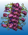
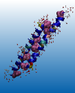
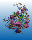
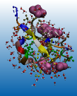
Figure 1: (Color online) Four different classes of considered AFP structures (from left to right): tenebrio molitor (1EZG) as used in Mao and Ba (2006), psodeupleuronectes americanus (1WFB) in Hobbs et al. (2011); Slaughter and Hew (1981), hemitripterus americanus (2AFP) in Gronwald et al. (1998), and macrozoarces americanus (1MSI) in Wang et al. (2012). Figures prepared with crystallographic data in RCSB Protein Data Bank.

The mechanism of AFP binding is still unresolved Hew and Yang (1992) since the details of the antifreeze effect are difficult to test experimentally, mainly because it is not easy to access them in their natural environment. Molecular dynamic simulations Nada and Furukawa (2012); Liu et al. (2012) are limited by the computing power and running times. Moreover the interaction between AFPs and the liquid-solid interface is determined by the choice of the water model and the potential parameters Guillot (2002); Berendsen et al. (1987, 1984); Svishchev and Kusalik (1996); Jorgensen et al. (1983); Kiss and Baranyai (2011); Stern et al. (2001); Mahoney and Jorgensen (2000); Essmann et al. (1995). The simple freezing point depression such as observed in saline solutions is proportional to the molal concentration of the solute molecule Yeh and Feeney (1996), where the colligative property does not depend on the structure of the molecules. However, a more careful inspection of AFPs shows a nonlinear dependence so that colligative effects are ruled out Nada and Furukawa (2012). We propose a dynamical mechanism for freezing point depression by AFPs leading to a nonlinear dependence on the AFP density.

There is not a single mechanism known up to date which explains the AFP ice-binding affinity and specificity Barrett (2001). One reason lies in the considerable variation of the primary, secondary and tertiary structure of AFPs Barrett (2001); Jia and L.Davies (2002); Yeh and Feeney (1996); Grunwald et al. (2009); Harding et al. (1999); Hew and Yang (1992) because the ice-binding affinity depends on the molecular recognition according to the key-lock principle Daley et al. (2002); Leinala et al. (2002). The different kinds of structures lead to various kinetic models of AFP activity Li et al. (2006, 2009); Burcham et al. (1986); Kristiansen and Zachariassen (2005); Kubota (2011); Wang et al. (2012); Sander and Tkachenko (2004). A significant difference can be found by the shape of the antifreeze activity between AFGP 4 and AFGP 8 Li and Luo (2000); Burcham et al. (1986). In addition to that, several authors have substituted threonine residues and have investigated the influence on the thermal hysteresis Zhang and Laursen (1998); Schrag et al. (1982) or have enhanced the activity of a $\beta$-helical antifreeze protein by engineered addition of coils Marshall et al. (2004); Mao and Ba (2006).

Moreover, other authors have assessed the relationship between the non-colligative freezing point depression and the molecular weight of AFPs Schrag et al. (1982); Raymond and de Vries (1977) and have observed cooperative functioning between the larger and the smaller components Osuga et al. (1978). The stabilization of supercooled fluids by thermal hysteresis proteins Wilson and Leader (1995); Zachariassen (1985) is discussed with a number of models based on kinetics, statistical mechanics and homogeneous or inhomogeneous nucleation Li et al. (2006, 2009); Li and Luo (1993); Kubota (2011); Li and Luo (1994, 2000); Liu and Li (2003, 2006); Wang et al. (2012); Sander and Tkachenko (2004); Mao and Ba (2006); Raymond and de Vries (1977). All these models describe a thermal hysteresis as a function of concentration, but no pattern formation in space and time during the phase transition from liquid water to ice. In contrast, the Turing model Kutschan et al. (2010) and the phase field model Thoms et al. (2013); Morawetz et al. (2014) simulate the morphology of the microstructural growth but without thermal hysteresis. Our main goal is to include kinetic models capable to describe the experimental observations into the phase field method and to justify the non-equilibrium stabilized supercooled liquid state of the hysteresis.

We use coupled phase field equations for the water-ice structure and the AFP concentration, which is connected with the question on how the protein structure influences antifreeze activity. The various phase field approaches differ in the choice of the bulk free energy density. We use the Gibbs free energy according to the classical Landau theory of a first-order phase transition as the freezing of water. This phenomenological free energy as a form of mean-field theory is expanded in a power series of the order parameter. The Landau coefficients describe the equilibrium as well as the metastable states of the ice/water system and can be deduced from properties of water as demonstrated in Thoms et al. (2013). A more microscopic approach has to rely on water models like density functionals, which are currently not simultaneously available for water and ice. We therefore restrict ourselves to three phenomenological parameters, which can be linked to known water properties.

The dynamical formation of the micro-structures are calculated by solving the coupled phase field equations which combine the phase field theory of Caginalp Caginalp (1986); Caginalp and Lin (1987); Caginalp and Fife (1988); Caginalp (1989, 1990, 1991), Cahn and Hilliard Gránásy et al. (2004); Gránásy (1999); Gránásy and Oxtoby (2000); Gránásy et al. (2002) with various kinetics Yeh and Feeney (1996); Burcham et al. (1986); Kubota (2011); Wang et al. (2012); Mao and Ba (2006). In the next section we outline shortly the basic equations and models. Then we present the nonlinear freezing point depression from static conditions and support this by numerical discussions of the time-dependence of freezing suppression.

II Coupling of AFP to ice structure

We begin with a phase field model Gránásy et al. (2004) with ice nucleation of Cahn-Hilliard-type proposed in Gránásy (1999), due to the lack of complete understanding of water by first principles. We identify the ice structure by an order parameter $u$ describing the ”tetrahedricity” Medvedev and Naberukhin (1987)

$$u\sim 1-M_{T}=1-\frac{1}{15<l^{2}>}\sum_{i,j}(l_{i}-l_{j})^{2},$$ (1)

where $l_{i}$ are the lengths of the six edges of the tetrahedron formed by the four nearest neighbors of the considered water molecule. For an ideal tetrahedron one has $M_{T}=0$ and the random structure yields $M_{T}=1$. In this way it is possible to discriminate between ice- and water molecules either by using a two-state continuous function. Other authors prefer the ”tetrahedrality” in order to define the order parameter Errington and Debenedetti (2001); Kumar and an H. Eugene Stanley (2009); Mason and Brady (2007). We adopted a quartic order parameter relationship of Ginzburg-Landau-type for the free energy density

$$f(u,v)\sim\beta u+\lambda u^{2}-2\lambda u^{3}+\lambda u^{4}+c\left(\frac{\partial u}{\partial x}\right)^{2}$$ (2)

allowing nonlinear structures to be formed. The fourth order function enables a double well potential for the description of the water-ice phase transition Harrowell and Oxtoby (1987). The coefficient $\lambda$ describes the free energy density scale and $\beta$ the deviation from equilibrium.

The versatile action of different molecular structures of AFPs on the grain growths is simulated by an activity parameter relating the structural order parameter to the antifreeze concentration $f(u,v)\sim-a_{1}uv$. The coefficient $a_{1}$ describes the interaction between the order parameter $u$ and the antifreeze concentration $v$. This approach is different from the description of simple freezing point depression in saline solutions Thoms et al. (2013); Morawetz et al. (2014) in that the AFPs act analogously to a magnetic field on charged particles thus providing a hysteresis.

We follow the philosophy of the conserving Cahn-Hilliard equation and assume that the time-change of the order parameter is proportional to the gradient of a current $\dot{u}=-\nabla j$. The current itself is assumed to be a generalized force, which in turn is given by the gradient of a potential, $j\sim\nabla\Phi$. The latter is the variation of the free energy such that finally $\dot{u}=-\nabla^{2}(-{\partial f\over\partial u})$ results. From the differential form for a general continuity equation $\frac{\partial v}{\partial t}+\frac{\partial j}{\partial x}=0$ with the AFP field $v$ and the flux $j=-\frac{\partial}{\partial x}\left(a_{3}v+a_{2}u\right)$ we get a diffusion equation $\frac{\partial v}{\partial t}=\frac{\partial^{2}}{\partial x^{2}}\left(a_{2}u+a_{3}v\right)$ as evolution for the AFP concentration. For further considerations we introduce the dimensionless quantities $\tau=\frac{t}{t_{0}}$, $\xi=\frac{x}{x_{0}}$, $u=C_{1}\hat{\psi}$, $v=C_{2}\rho$, with $C_{1}=1$, $C_{2}=\frac{a_{1}}{12\lambda}$, $x_{0}=\frac{1}{6}\sqrt{\frac{6c}{\lambda}}$, $t_{0}=\frac{c}{72\lambda^{2}}$ with $\alpha_{1}=\frac{a^{2}_{1}}{12^{2}\lambda^{2}}$, $\alpha_{2}=\frac{a_{2}}{12\lambda}$ and $\alpha_{3}=\frac{c\beta}{72\lambda^{2}}$ such that the order-parameter and the AFP concentration equations read

$$\frac{\partial\psi}{\partial\tau}\! = \!\frac{\partial^{2}}{\partial\xi^{2}}\!\left(\!\alpha_{3}\!+\!\left(\frac{1}{6}\!-\!a\!+\!a^{2}\right)\psi\!+\!\left(a\!-\!\frac{1}{2}\right)\psi^{2}\!+\!\frac{1}{3}\psi^{3}\right.$$ (3)

$$\left.-\alpha_{1}\rho-\frac{\partial^{2}\psi}{\partial\xi^{2}}\right)$$

$$\frac{\partial\rho}{\partial\tau} = \frac{\partial^{2}}{\partial\xi^{2}}\left(\psi+\alpha_{2}\rho\right).$$ (4)

We have shifted $\psi=\hat{\psi}-a$ by technical reasons since $a=1/2$ allows the removal of the cubic term in the free energy.

The Cahn-Hilliard equation cannot be derived from the Onsager reciprocal theorem Wheeler (1993) because the Markovian condition is not satisfied Emmerich (2003), but has the virtue of a conserving quantity. It possesses a stationary solution, which can be seen from the time evolution of the total free energy Bestehorn (2006)

$${d\over dt}\int fdV = \int{\delta f\over\delta\psi}{d\psi\over dt}dV=\int{\partial f\over\partial\psi}\nabla^{2}({\partial f\over\partial\psi})dV$$ (5)

$$= -\int\left(\nabla{\partial f\over\partial\psi}\right)^{2}dV\leq 0.$$

III Mechanism of freezing point depression

III.1 Phase diagram

We analyze the static solution of (3) and (4) eliminating $\rho=-\psi/\alpha_{2}$ and obtain

$$\frac{\partial^{2}\psi}{\partial\xi^{2}}=\alpha_{3}-\aleph\psi-\left(a-\frac{1}{2}\right)\psi^{2}+\frac{1}{3}\psi^{3}\equiv\frac{\partial\phi}{\partial\psi}$$ (6)

which can be understood as the Euler-Lagrange equations from the free energy

$$f =\alpha_{3}\psi-\aleph{\psi^{2}\over 2}+\left(a-\frac{1}{2}\right){\psi^{3}\over 3}+\frac{1}{12}{\psi^{4}}+\frac{1}{2}\left(\frac{\partial\psi}{\partial\xi}\right)^{2}$$

$$\equiv\phi+\frac{1}{2}\left({\partial\psi\over\partial\xi}\right)^{2}$$ (7)

where we abbreviate $\aleph=-\frac{1}{6}+a-a^{2}-\frac{\alpha_{1}}{\alpha_{2}}$. Eq. (6) is easily integrate by multiplying both sides with $\partial\psi/\partial\xi$ to yield

$$\frac{1}{2}\left(\frac{\partial\psi}{\partial\xi}\right)^{2}=\phi+c\equiv\Phi$$ (8)

providing the virial theorem $f=2\phi+c=2\Phi-c=(\psi^{\prime})^{2}-c$ as an expression for the conservation of energy. This fact allows us to calculate the static profile of the kink solution as shown. Depending on the parameter $\alpha_{1}/\alpha_{2}$ and $\alpha_{3}$ we obtain an asymmetric potential $\Phi$ describing the thermodynamic hysteresis though $\alpha_{3}$ does not influence the dynamics due to the differentiation in Eq. (3). Near the phase transition the potential $\Phi$ becomes symmetric and possesses a reflection symmetry $\Phi(\psi)=\Phi(-\psi)$ with the minimum $\psi_{min}=\pm\sqrt{3\aleph}$. Hence, the constant $c$ can be found from the condition $\Phi(\sqrt{3\aleph})=-\frac{3}{4}\aleph^{2}+c=0$.

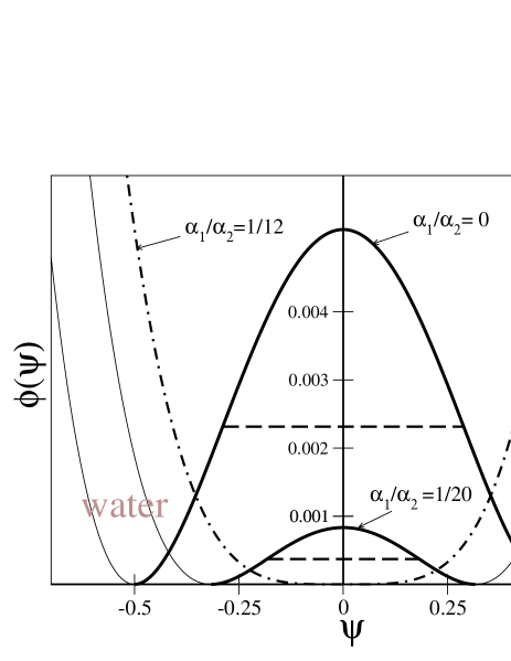
Figure 2: Free energy density (solid) versus order parameter for different AFP concentrations, pure ice/water $\frac{\alpha_{1}}{\alpha_{2}}=0$ (upper line). The freezing transition interval is given by $\partial^{2}\phi/\partial\psi^{2}=0$ (dashed lines).

In figure 2 the symmetric potential is plotted where the left and right minima reflect the stable phase of water and ice respectively. The concave $\partial^{2}\Phi/\partial\psi^{2}<0$ region corresponds to a negative diffusion coefficient leading to structure formation. The flux diffuses up against the concentration gradient contrary to the Onsager reciprocal theorem Wheeler (1993) and which is the unstable phase transition region. This freezing region is reduced by the AFP concentration where for $\frac{\alpha_{1}}{\alpha_{2}}=\frac{1}{12}$ the double well vanishes.

III.2 Linear stability analysis

It is also possible to compute the phase transition region with the help of the positive eigenvalues $\mu$ of the linear stability analysis around the equilibrium value $\psi=\psi_{0}+\psi_{0}\exp(\mu\tau+i\kappa\xi)$ and $\rho=\rho_{0}+\rho_{0}\exp(\mu\tau+i\kappa\xi)$ with the wavenumber $\kappa$ and the fixed point $\psi_{0}$. Each fixed point describes a spatial homogeneous order parameter $\psi=\psi_{0}=const$ and corresponds to a stationary solution of water or ice. For pure water ($\alpha_{1}=0$) of (3) the range of unstable homogeneous solution is

$$\mu^{*}(\kappa)=\left(\aleph-\psi^{2}_{0}\right)\kappa^{2}-\kappa^{4}>0$$ (9)

and a perturbation grows in time and therefore establishes a spatial structure. For the complete equation system (3) and (4) with thermal hysteresis proteins (AFPs), one obtains the eigenvalues

$$\mu(\kappa)=-\frac{1}{2}(\alpha_{2}\kappa^{2}\!-\!\mu^{*}(\kappa))\!\pm\!\frac{1}{2}\sqrt{(\alpha_{2}\kappa^{2}\!+\!\mu^{*}(\kappa))^{2}\!-\!4\alpha_{1}\kappa^{4}}.$$ (10)

The region of positive eigenvalues corresponds to the freezing (spinodal) region. The unstable modes vanish for $\psi^{2}_{0}>{1/12}$ and also the double well for ${\alpha_{1}/\alpha_{2}}>{1/12}$. A phase transition occurs only, if the fixed points are located inside of $-{1/\sqrt{12}}<\psi_{0}<{1/\sqrt{12}}$ being also inside the freezing (spinodal) interval in Fig. 2. Since $\sqrt{\aleph}=\psi_{0}$ at the inflection points it can be concluded from Eq. (9)

$$\kappa^{2}+\psi_{0}^{2}-\left(\frac{1}{12}-\frac{\alpha_{1}}{\alpha_{2}}\right)\psi_{0}<0$$ (11)

forming an elliptic paraboloid as phase diagram in figure 3. The size of the microstructure is coupled to the AFP concentration and to the order parameter $\psi_{0}$ which decides how much ice and water is present. The freezing region shrinks with increasing AFP concentration and vanishes at $\alpha_{1}/\alpha_{2}=1/12$.

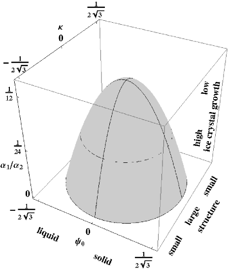
Figure 3: Freezing (spinodal) region dependent on the order parameter $\psi_{0}$ and the wavenumbers $\kappa$ and the thermal hysteresis activity $\frac{\alpha_{1}}{\alpha_{2}}$.

III.3 Surface energy depression

The virtue of the Cahn Hilliard equation (3) is the existence of a transient stationary solution by integrating (8) in form of a kink solution

$$\psi(\xi)=-\sqrt{3\aleph}\tanh\left[\sqrt{\aleph/2}(\xi-\xi_{0})\right]$$ (12)

with $\aleph=\frac{1}{12}-\frac{\alpha_{1}}{\alpha_{2}}$ as plotted in figure 4. The corresponding interfacial energy density of the kink is easily evaluated using the centered free energy density $\epsilon(\xi)=f(\xi)-c=({\partial\psi\over\partial\xi})^{2}$ plotted as well in figure 4.

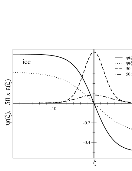
Figure 4: Static kink solution (12) and the interfacial energy density $\varepsilon(\xi)$ on the interface with AFPs ($\frac{\alpha_{1}}{\alpha_{2}}=0.05$) and without AFPs ($\frac{\alpha_{1}}{\alpha_{2}}=0$).

One recognizes that the presence of AFPs reduces the kink between water and ice and lowers the interfacial energy density. This is already a static mechanism which shows how the AFPs inhibit the formation of large ice clusters. The interfacial surface energy (tension)

$$\zeta=\int\limits^{\infty}_{-\infty}\varepsilon(\xi)d\xi=(2\aleph)^{3/2}$$ (13)

decreases with increasing AFP coupling and finally vanishes at the critical value $\alpha_{1}/\alpha_{2}=$1/12 which is the limit of the stability region. Transforming back to the dimensional interfacial energy one obtains $6^{3/2}\gamma\zeta$ with our choice of the surface tension $\gamma=21.9\frac{mJ}{m^{2}}$ Gránásy (1999). Direct and indirect measurements provide values which vary between $20\frac{mJ}{m^{2}}$ and $46\frac{mJ}{m^{2}}$ Jones (1974). In contrast to antifreeze proteins, $\gamma$ increases linearly with the salt concentration and a larger critical nucleus is required in order to generate an interface compared to pure water. Salt inhibits the nucleation process because of the higher energy threshold whereas thermal hysteresis proteins (AFPs) reduce the threshold for a stable nucleus. From this effective surface tension one might fix the ratio of materials parameter $\aleph=1/12-\alpha_{1}/\alpha_{2}$.

An ice crystal forms when the aqueous phase undergoes supercooling below the freezing point. In the supercooled phase water can transform from the aqueous to the solid phase by the growth of nucleation kernels if a critical size is exceeded. This critical radius separates the reversible accumulation of ice molds (embryos) from the irreversible growth of ice crystal. The nucleation process happens in two steps. As soon as the nucleation embryo overcomes the critical size it starts growing irreversibly. This is a dynamical process which we will consider below. One can estimate the critical radius within a simple liquid drop model. The volume part of Gibb’s potential is negative $\sim-{4\pi r^{3}}\Delta G_{V}/3$ while the surface part contributes positively $\sim 4\pi r^{2}\zeta$. Therefore Gibb’s potential exhibits a maximum at the critical cluster size $r^{\ast}={2\zeta}/{\Delta G_{V}}.$ As long as $r<r^{\ast}$ nucleation might happen (embryo) but no cluster grows for which case the critical cluster size has to be exceeded. This interfacial energy of the critical nucleus and the degree of supercooling are essentially influenced by the AFPs. Indeed the change of the free energy between ice and water $\psi(\pm\infty)=\pm\sqrt{3\aleph}$ reads with the stationary solution (12)

$$\Delta F=-2(\alpha_{3}-\alpha_{1}\rho)\sqrt{3\aleph}\approx\Delta G_{V}.$$ (14)

With (13) the critical (dimensionless) radius $r^{\ast}={\sqrt{2\aleph}/3(\alpha_{1}\rho-\alpha_{3})}$ decreases as the AFP concentration $\alpha_{1}/\alpha_{2}$ increases. In other words more AFPs allow more ice nucleation but inhibit the cluster growth.

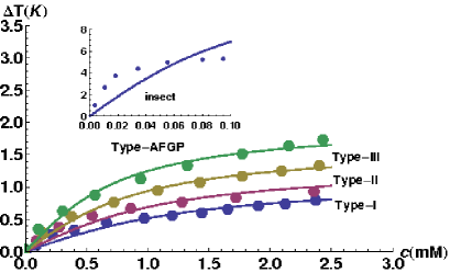
Type	I	II	III	AFGP	insects
a	0.81	1.08	2.58	4.31	34.39
b	0.44	0.37	0.88	1.13	0.05

Figure 5: (Color online) The freezing temperature depression of four different classes of AFP structures Wang et al. (2012); Gronwald et al. (1998); Hobbs et al. (2011) and insects Mao and Ba (2006) versus AFP concentration where (16) is used (lines) to fit the experimental data (points) of the collected data in Nada and Furukawa (2012). The AFP-specific fitting parameter are given in the table.

III.4 Freezing point depression

The decrease of the freezing temperature $\Delta T$ can be estimated by the change of the free energy during the phase transition since the corresponding minima of the asymmetric free energy are nearly the same as the ones of the symmetric free energy (14). We can write

$$\left.\Delta F\right|_{\rm ice-water}=\left.{\partial F\over\partial T}\right|_{\rm ice}\Delta T$$ (15)

for constant particle number and pressure. We model the temperature dependence of the coupling between AFP concentration and ice structure as $\alpha_{1}(T)=\alpha_{0}+\alpha_{10}(T-T_{c}^{0})$ with some internal threshold temperature $T_{c}^{0}$. The activity of AFP molecules will certainly be temperature dependent and cease to act at the critical temperature $\alpha_{1}(T^{*})=0$. Therefore the freezing point depression is given by $\Delta T=T^{*}-T_{c}^{0}$. Introducing the AFP-dependent supercooling temperature $T_{c}=T_{c}^{0}-|\Delta T|$ one may write $\alpha_{1}(T)=\alpha_{0}(T-T_{c})/|\Delta T|$. From (15) and (14) we obtain the freezing point depression or thermodynamical hysteresis observing $\psi|_{\rm ice}=\sqrt{3\aleph}$ as

$$|\Delta T|=\sqrt{\left({b\over 2\rho}\right)^{2}+a}-{b\over 2\rho}$$ (16)

with $a=2\alpha_{0}(T-T_{c})/\alpha_{10}$ and $b=2\alpha_{3}/\alpha_{10}$. We see a nonlinear square root behavior of the freezing point depression which is dependent on the AFP concentration $\rho$ which expands for small concentrations $|\Delta T|\approx{a\over b}\rho={\alpha_{0}\over\alpha_{3}}(T-T_{c})\rho$ into a colligative freezing depression analogously as known from saline solutions. The nonlinear behavior fits well with the experiments as seen in figure 5. The fit parameters can be translated into two conditions for the four materials parameter $\alpha_{3},\alpha_{10},\alpha_{0}$ and $T_{c}$ for each specific AFP. Together with the surface tension our approach leaves one free parameter to describe further experimental constraints.

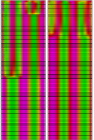
Figure 6: (Color online) Time evolution of the order parameter versus length from $1\times 10^{5}$ to $2\times 10^{6}$ time steps (from above to below), left side without AFPs and right side with AFPs.

III.5 Time evolution of ice growth inhibition

Now that we have seen how the AFP reduces the interfacial energy and therefore the formation of ice crystals we turn to investigate the time evolution. We use the exponential time differencing scheme of second order (ETD2) Cox and Matthews (2002) with the help of which a stiff differential equation of the type $y^{\prime}=ry+z(y,t)$ with a linear term $ry$ and a nonlinear part $z(y,t)$ can be integrated. The linear equation is solved formally and the integral over the nonlinear part is approximated by a proper finite differencing scheme. The time evolution of the coupled equations (3) are seen in figure 6. Due to the Cahn Hilliard equation we have conservation of total mass density of water $\rho_{w}$ but a relative redistribution between water $\rho_{liq}$ and ice $\rho_{ice}$ densities which read in terms of the ice order parameter $\rho_{w}(\xi,t)=\rho_{liq}[1-\psi(\xi,t)]+\rho_{ice}[1+\psi(\xi,t)]$. Since the total integral over the order parameter $\int\psi(\xi,t)d\xi=const$ the mass conservation of water is ensured.

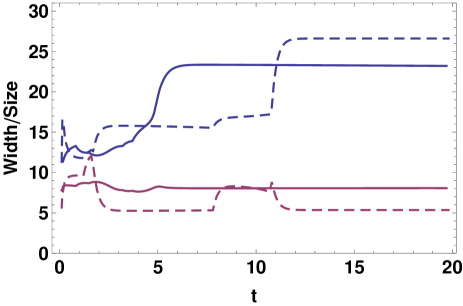
Figure 7: (Color online) The half width of ice structure (upper curves) together with the thickness of the boundary (lower curves) without (dashed) and with AFPs (solid) of the time evolution of order parameter from figure 6.

In figure 6 we plot the time evolution of an initially small-scale distributed sinusoidal order parameter with and without AFPs. The evolution equations obviously reduce the number of ice grains forming a larger one after some time. Interestingly this accumulation occurs faster with AFPs than without. However, as we have already seen, the absolute height of the ice-order parameter (ideal ice corresponds to $\Psi=1$) is lowered by AFPs during this process.

This is also illustrated by the time-evolution of the half width of the kinks in figure 7 which we interpret as the size of the ice grains. One sees that the grain size of ice evolves faster with AFPs and remains at a smaller value compared to the case without AFPs. This means the nucleation of ice starts earlier with AFPs but remains locked at an intermediate stage. This is in agreement with the static observation above that the AFPs support smaller nuclei sizes and inhibit the formation of large clusters at the freezing point. We consider this later blocking of larger cluster sizes as an dynamic process due to the kinetics and coupling of AFPs to the ice embryos described here by a linear term in the free energy. Accompanying this observation we also see that the width of the boundary between ice and water remains larger with AFPs than without. This is of course an expression of the reduction of interfacial energy.

IV Summary

The interaction of AFP molecules with ice crystals is described by a coupled phase field equation between the order parameter describing ice and water and the AFP concentration. We find essentially two effects of AFPs in suppressing the formation of ice crystals. First the interfacial energy is lowered which allows only smaller ice nuclei to be formed. And secondly we see that the ice grains are formed faster by the action of AFPs but become locked at smaller sizes and smaller order parameters. The latter means that the freezing is stopped and ice-water mixture remains instead of completely freezing. According to the proposed model the AFPs do not prevent crystal nucleation, but inhibit further growth of the initial crystal nuclei. This essentially dynamic process between AFP structure and ice-order parameter establishes a new possible mechanism for the phenomenon of anti-freeze proteins. We demonstrate that the model is capable to reproduce the experimental data on the freezing point depression in principle. The used phenomenological parameters can be linked to known properties of water Thoms et al. (2013) though a more microscopic determination of these parameters is highly desired but out of the scope of this paper.