Upper-bounding bias errors in satellite navigation

Abstract

A satellite navigation system for a safety critical application is required to provide an integrity alert of any malfunction; the probability that a navigation positioning error exceeds a given alert limit without an integrity alert is required to be smaller than a given integrity risk. So far, a little number of applications provide integrity alerts, because signal propagation from a satellite to a receiver depends on diversified phenomena and makes probabilistic upper-bound of possible threats difficult. To widen application fields of satellite navigation, two methods to upper-bound wide classes of bias errors are shown in this paper. The worst bias error in a maximum likelihood estimate caused by an interference signal within a given small power is derived. A novel inequality condition with a clock bias error and magnification coefficients that upper-bounds a horizontal position error is presented. Robustness of the inequality condition is numerically shown based on actual configurations of satellites.

Index Terms—  Integrity, satellite navigation system, safety critical application, bias error, maximum likelihood estimate

1 Introduction

Satellite navigation systems have been tried on safety critical applications in various fields. One of the most successful applications is the Satellite Based Augmentation System (SBAS). It was commissioned for aviation in USA in 2003 [1] and is planned to cover large parts of the globe around 2020 [2]. SBAS provides integrity alerts to contain the probability of Hazardously Misleading Information below a given integrity risk. For example, the category of Approach Procedures with Vertical Guidance I (APV-I) requires that the probability that a vertical navigation positioning error exceeds the alert limit of 50 m without integrity alerts should be less than $2\times 10^{-7}$ per approach.

SBAS bases on over-bounding statistics that are designed to cover potential threats with sufficient margins. For example, orbit and clock errors of Global Positioning System (GPS) are investigated over a considerable period and over-bounding distributions are provided [3]. Multipath errors at antennas on airplanes are also modeled and simulated [4] and taken into consideration of standard multipath powers as functions of parameters such as an elevation angle of a satellite [5].

Besides aviation, applications to other fields including railways are being tried [6]. Near surface, however, serious and diversified errors caused by multipaths have been reported [7]. Since multipath errors show strong dependences on each propagation environment, no distributions are confirmed to over-bound multipath errors, so far. When sufficient statistics are not available, additional sensors are expected to overcome threats. It was pointed out that a precise clock of a receiver works to detect an error in an estimate of clock bias that has correlation with an error in an estimate of vertical position [8]. In the same literature, a horizontal position error was denoted as essentially uncorrelated with an estimate of a clock bias error.

In this paper, two methods to upper-bound bias errors are shown. The worst bias error in a maximum likelihood estimate caused by an interference signal within a given small power is derived in a simple expression in Section 2. It gives fast estimation of the worst bias error once the power of an interference signal becomes available as in [5]. In Section 3 a novel inequality condition with a clock bias error and magnification coefficients that upper-bounds a horizontal position error is presented. Robustness of the inequality condition is numerically evaluated based on an ephemeris of GPS satellites in Section 4 and the conclusion follows.

2 The worst bias error caused by an interference within a given small power

A general framework of the worst bias error in a maximum likelihood estimate caused by an interference signal within a given small power is presented in [9]. For a cord spread signal as used in GPS, it is further possible to express and evaluate the worst mode explicitly as follows. Suppose that a signal is periodically sampled at $kT$ for $k=1,2,...$, where $T$ is a sampling period, and modeled by

$$z(kT)=w(kT-\tau)+y(kT)+n(kT),$$ (1)

where $w(kT-\tau)=re^{i\phi}m(kT-\tau)$ is a known code $m(kT-\tau)\in\mathbb{R}$ with an unknown delay $\tau\in\mathbb{R}$ multiplied by an amplitude $r$ and a phase $e^{i\phi}$, and $y(kT)$, $n(kT)\in\mathbb{C}$ are respectively an interference signal and a noise independently obeying a Gaussian distribution density

$$p(n(kT))=\frac{1}{\sqrt{2\pi}\sigma}\exp\left(-\frac{|n(kT)|^{2}}{2\sigma^{2}}\right).$$ (2)

The logarithmic likelihood function of parameters with respect to samples is derived as $L_{y}=\sum_{k}\ell_{y,k}$ with

Let $\tau_{0}$ denote the maximum likelihood estimate of the delay for the unperturbed ($y=0$) system,

$$\frac{\partial L_{0}}{\partial\tau}(\tau_{0})=0,$$ (4)

and $\tau_{0}+\delta\tau$ is the one for the perturbed system with a small $\delta y$. The condition

$$\frac{\partial L_{\delta y}}{\partial\tau}(\tau_{0}+\delta\tau)=0$$ (5)

gives an explicit representation

where $w^{\prime}$ denotes the derivative of $w$, $z^{\ast}$ denotes the complex conjugate of $z$, and c.c. denotes the complex conjugate of the previous term. Straightforward calculation up to the first order gives

$$|\delta\tau| =\left|\frac{\langle\delta y,w^{\prime}\rangle}{\|w^{\prime}\|^{2}+\langle w-z,w^{\prime\prime}\rangle}\right|$$ (7)

$$\leq M_{\tau}\|\delta y\|,$$ (8)

with the magnification coefficient defined by

$$M_{\tau} :=\frac{\|w^{\prime}\|}{\left|\|w^{\prime}\|^{2}+\langle w-z,w^{\prime\prime}\rangle\right|},$$ (9)

where $\langle a,b\rangle:=\sum_{k}a(k)^{\ast}b(k)$ denotes the inner product of complex vectors $a$ and $b$ of the same dimension, $\|\delta y\|=\sqrt{\langle\delta y,\delta y\rangle}$ is the square root of a power of an interference signal $\delta y$, and $w^{\prime\prime}$ denotes the second derivative of $w$. The equality holds for the interference signal $\delta y$ parallel to $w^{\prime}$. This worst mode corresponds to the Goldstone mode with respect to the time translational symmetry [10] and gives fast estimate of the worst error caused by an interference within a given small power regardless of details, once the power of interference becomes available.

3 Upper-Bounding bias errors in horizontal position estimates

The observation equation of a pseudo range

$$\delta\rho_{j}=\langle\bm{g}_{j},\delta\bm{x}\rangle+\delta b+\epsilon_{j},$$ (10)

is derived by linearizing a pseudo range $\rho_{j}$ from the $j$-th navigation satellite ($j=1,2,\ldots$) reaching a base point $\bm{x}_{0}$ at a base time $t_{0}$ for a neighborhood $(\bm{x}_{0}+\delta\bm{x},t_{0}+\delta b/c)\in\mathbb{R}^{4}$, where a geometry vector $\bm{g}_{j}\in\mathbb{R}^{3}$ is the unit direction vector to the $j$-th satellite form the base point $\bm{x}_{0}$ multiplied by $-1$, $\epsilon_{j}$ is an correction term on the pseudo range form the $j$-th satellite, $b$ is called a bias, and $c$ denotes the light velocity.

Suppose that a position of an antenna is limited in a curve $\bm{x}(s)=(x(s),y(s),z(s))\in\mathbb{R}^{3}$ that is continuous and an almost everywhere differentiable function of the distance $s$ from the base point (Fig. 1 (a)). Let $\bm{U}$ and $\bm{V}$ be the tangential unit vector of the curve and the unit vector to the center of the osculating circle that is tangential to the curve at the point $\bm{x}(s)$ respectively, and $\bm{W}$ be the unit vector that consists of a orthogonal frame with $\bm{U}$ and $\bm{V}$, which is called the Frenet frame (Fig. 1 (b)).

(a) An example of a railway curve (Brusio spiral viaduct [11]).

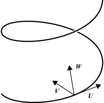
(b) The Frenet frame on a curve.

Fig. 1: An example of a frame on a railway curve.

Against this frame a deviation is expressed as $\delta\bm{x}=\delta u\bm{U}+\delta v\bm{V}+\delta w\bm{W}$. The curve is approximated by the osculating circle, whose radius is denoted by $R$, in a neighborhood of $\bm{x}(s)$ as

$$(u(s),v(s))=R\left(\sin\frac{s}{R},1-\cos\frac{s}{R}\right).$$ (11)

Under this approximation, a projection from the point $(u,v)$ measured from the navigation satellites to the distance parameter $s=R\arctan\left(u/(R-v)\right)$ is derived for the domain $v<R$ and linearized for small deviations

When three satellites $j=1,2,3$ are available, it is derived from the observation equation

$$\left[\begin{array}[]{c}\delta\rho_{1}\\ \delta\rho_{2}\\ \delta\rho_{3}\end{array}\right]=\left[\begin{array}[]{ccc}f_{1}&h_{1}&1\\ f_{2}&h_{2}&1\\ f_{3}&h_{3}&1\\ \end{array}\right]\left[\begin{array}[]{c}\delta u\\ \delta v\\ \delta b\end{array}\right]+\left[\begin{array}[]{c}\epsilon_{1}\\ \epsilon_{2}\\ \epsilon_{3}\end{array}\right],$$ (13)

where directional cosines are denoted by $f_{j}:=\langle\bm{g}_{j},\bm{U}\rangle$, $h_{j}:=\langle\bm{g}_{j}\bm{V}\rangle$ respectively. When the condition on satellites configuration

$$D:=f_{1}h_{2}-f_{2}h_{1}+f_{2}h_{3}-f_{3}h_{2}+f_{3}h_{1}-f_{1}h_{3}\neq 0$$ (14)

holds, the equation

holds. When the correct value of each correction $\epsilon_{j}$ is substituted, this equation represents the change of coordinates $(\delta u,\delta v,\delta b)$ against the change of each pseudo range $\delta\rho_{j}$. If some correction is not included correctly, then the output contains error.

Empirical distributions of orbit and clock errors of navigation satellites shows good convergence to the stationary one [3]. There are also augmentation services to monitor orbit and clock errors. Thus it is well assumed that those errors are over-bounded by a certain distribution and its scale can be neglected later in this paper, when larger residuals are discussed.

Besides above mentioned, ionospheric delay, tropospheric delay, diffraction of signals, and reflection of signals are major sources of errors. All these physical effects make positive contribution to the correction term $\epsilon_{j}>0$; if not all are substituted, there remains error $r_{j}:=\delta\rho_{j}-\epsilon_{j}>0$.

For $j=1,2,3$ complex numbers $z_{j}:=f_{j}+ih_{j}$ and $z_{4}=z_{1}$ satisfy an equation $\operatorname{Im}(z_{j}^{\ast}z_{j+1})=f_{j}h_{j+1}-f_{j+1}h_{j}$. There exists complex numbers that satisfy the condition $\operatorname{Im}(z_{1}^{\ast}z_{1}z_{2}^{\ast}z_{2}z_{3}^{\ast}z_{3})=0$ subject to the condition $\operatorname{Im}(z_{j}^{\ast}z_{j+1})>0$ under suitable exchanges of suffixes. For satellites satisfying the above condition, an upper bounding inequality for an error along a track

$$|\delta u| =\left|\frac{(h_{2}-h_{3})r_{1}+(h_{3}-h_{1})r_{2}+(h_{1}-h_{2})r_{3}}{D}\right|$$ (16)

$$\leq M_{u}|\delta b|$$ (17)

and one for perpendicular to a track

$$|\delta v| \leq M_{v}|\delta b|$$ (18)

are derived, where magnification coefficients are defined by

On the curve whose radius $R$ is large enough, positioning error in the direction perpendicular to the curve does not affect an along track error effectively. In those cases, by introducing a virtual satellite $j=3$ to cancel the perpendicular error, only two physical satellites are needed for positioning and its evaluation as shown below. For a sufficient large $h_{3}$, the equation

$$\left[\begin{array}[]{c}\delta\rho_{1}\\ \delta\rho_{2}\\ \delta\rho_{3}\end{array}\right]=\left[\begin{array}[]{ccc}f_{1}&h_{1}&1\\ f_{2}&h_{2}&1\\ 0&h_{3}&0\\ \end{array}\right]\left[\begin{array}[]{c}\delta u\\ \delta v\\ \delta b\end{array}\right]+\left[\begin{array}[]{c}\epsilon_{1}\\ \epsilon_{2}\\ \epsilon_{3}\end{array}\right]$$ (20)

is considered. For the configuration of satellites satisfying the determinant condition $D^{\prime}:=f_{2}-f_{1}\neq 0$, the equation

holds. Arguments parallel to the previous on gives necessary conditions, either $f_{2}>0$ and $f_{1}<0$, or $f_{2}<0$ and $f_{1}>0$. When one of the conditions is holds, formally in the limit of $h_{3}\rightarrow\infty$ with a magnification coefficient

$$M_{s} :=\frac{1}{\min(|f_{1}|,|f_{2}|)},$$ (22)

an upper-bounding inequality along a track is derived as

$$|\delta s| \leq M_{s}|\delta b|.$$ (23)

Note that this result is consistent with one from a system

$$\left[\begin{array}[]{c}\delta\rho_{1}\\ \delta\rho_{2}\end{array}\right]=\left[\begin{array}[]{cc}f_{1}&1\\ f_{2}&1\end{array}\right]\left[\begin{array}[]{c}\delta s\\ \delta b\end{array}\right]+\left[\begin{array}[]{c}\epsilon_{1}\\ \epsilon_{2}\end{array}\right].$$ (24)

4 Numerical evaluation

The magnification coefficient $M_{s}$ defined in the previous section is calculated from an ephemeris on 25 July 2013 (Universal Time). Satellite positions are converted into local coordinates at the point on a railway (latitude 34.75337, longitude 135.42783, height 3.7m) laid almost straight in East-West direction near our factory in Amagasaki, Japan. Magnification coefficients at every 60 seconds are calculated on satellites with an elevation mask of 15 degree, and plotted against time in Fig. 2.

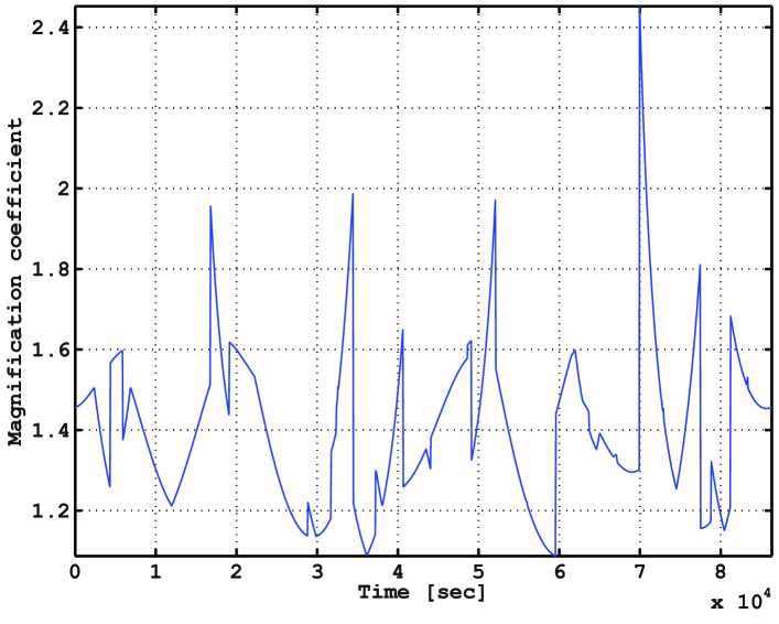
Fig. 2: The magnification coefficient calculated from the ephemeris on 25 July 2013 against every 60 seconds.

Sharp transitions in magnification coefficient values are caused by appearance or disappearance of satellites and thus depend on the selection of an elevation mask. Relative frequency of the magnification coefficients are plotted in Fig. 3.

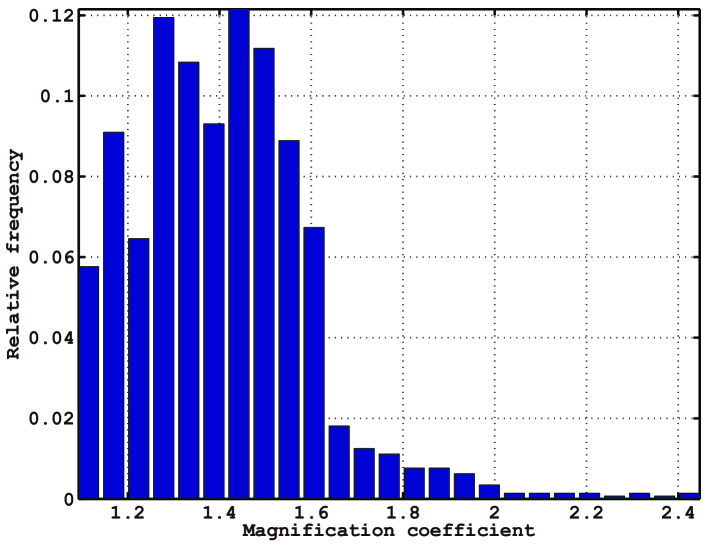
Fig. 3: Relative frequency of the magnification coefficients calculated for the ephemeris on 25 July 2013.

It is observed that most magnification coefficients are contained under the value 2 and concentrated under the value 1.6.

The accuracy of a local clock depends on its mechanism and calibration scheme. There are wide range of choices including a rubidium clock whose frequency stability is demonstrated less than $4\times 10^{-12}\tau^{-1/2}$ up to $10^{4}$ sec [12].

5 CONCLUSION

In this paper two methods to upper-bound bias errors have been shown. The worst bias error in maximum likelihood estimates caused by an interference signal within a given small power is represented. It gives a fast evaluation of an error caused by an interference regardless of details, once the power of interference becomes available. A novel inequality condition that upper-bounds a horizontal position error with a clock bias error and magnification coefficients is also shown. Robustness of the inequality conditions are shown based on actual constellation of satellites. Although optimization of a local clock as well as its calibration scheme and evaluation of system performance are remained for future work, these upper-bounds are expected to provide concrete bases for wide fields of safety critical applications.

References

- [1] Global positioning system with wide are augmentation system (WAAS) performance standard, Federal Aviation Administration, Washington D. C., 2008.
- [2] D. Thomas, “GNSS Evolution Program Update,” in Interoperability working group meeting (IWG), 2014.
- [3] C. Cohenour and F. van Graas, “GPS Orbit and Clock Error Distributions,” NAVIGATION: Journal of the Institute of Navigation, vol. 58, no. 1, pp. 17–28, 2011.
- [4] M. Lentmaier, B. Krach, T. Jost, A. Lehner, and A. Steingass, Assessment of multipath in aeronautical environments, Citeseer, 2008.
- [5] Propagation data required for the design of Earth-space aeronautical mobile telecommunication systems, International Telecommunication Union, ITU-R P. 682-3, 2012.
- [6] A. Ferrario, L. Marradi, P. Iacone, and A. Galimberti, “Multi-constellation GNSS Receiver for Rail Applications,” in ION GNSS+, 2013.
- [7] A. Steingass and A. Lehner, “Measuring the navigation multipath channel a statistical analysis,” in ION GPS 2004 Conference, 2004.
- [8] S. Bednarz and P. Misra, “Receiver clock-based integrity monitoring for GPS precision approaches,” IEEE Transactions on Aerospace and Electronic Systems, vol. 42, no. 2, pp. 636–643, 2006.
- [9] T. Wada and T. Iwamoto, “Evaluation of bias errors in positioning a radio transmitter with a lot of interference waves,” in Phased Array Systems and Technology (ARRAY), IEEE, 2010, pp. 1033–1038.
- [10] P. W. Anderson, Basic notions of condensed matter physics, Benjamin, 1984.
- [11] Gubler, “Picture taken near Brusio, Switzerland,” http://www.bahnbilder.ch/picture/11543, Creative Commons Attribution 3.0 Unported.
- [12] C. Affolderbach, F. Droz, and G. Mileti, “Experimental Demonstration of a Compact and High-Performance Laser-Pumped Rubidium Gas Cell Atomic Frequency Standard,” IEEE Transactions on Instrumentation and Measurement, vol. 55, no. 2, pp. 429–435, 2006.