Quench between a Mott insulator and a Lieb-Liniger liquid

Abstract

In this work we study a quench between a Mott insulator and a repulsive Lieb-Liniger liquid. We find explicitly the stationary state when a long time has passed after the quench. It is given by a GGE density matrix which we completely characterize, calculating the quasiparticle density describing the system after the quench. In the long time limit we find an explicit form for the local three body density density density correlation function and the asymptotic long distance limit of the density density correlation function. The latter is shown to have gaussian decay at large distances.

I Introduction

The question of whether an isolated quantum system equilibrates is of fundamental interest to our understanding of nonequilibrium dynamics. This question is extremely difficult to study in the condensed matter context as there are few truly isolated systems. However recent advances in the study of ultracold atoms have brought this question to the forefront. Thanks to an unprecedented amount of tunability and isolation in cold atom systems it has become possibly to study complex nonequilibrium dynamics of many body systems. Triggered by spectacular experimental advances key-1 (2, 5, 1, 3, 6, 7, 8, 4, 9) there has been great effort recently in the theoretical study of thermalization of isolated systems key-12 (10, 11, 12, 13, 14, 15, 16, 17, 18). The most important questions asked are whether a system equilibrates, what are the dynamics of the equilibration process and what ensemble if any describes the long time limit of an isolated system?

One of the most surprising recent experimental and theoretical results is that at long times the quenched Lieb-Liniger gas key-9-1 (19) retains memory of its initial state key-10-1 (20, 18, 1) and does not appear to relax to thermodynamic equilibrium. This is due to the fact that the Lieb Liniger hamiltonian:

$$H_{LL}=\intop_{-\infty}^{\infty}dx\left\{\partial_{x}b^{\dagger}\left(x\right)\partial_{x}b\left(x\right)+c\left(b^{\dagger}\left(x\right)b\left(x\right)\right)^{2}\right\},$$ (1)

has an infinite number of conserved charges $I_{i}$. Here $b^{\dagger}\left(x\right)$ is the bosonic creation operator at the point $x$ and $c$ is the coupling constant. These conserved quantities in turn imply that there is a complete system of eigenstates for the Lieb Liniger gas which may be parametrized by sets of rapidities $\left\{k_{i}\right\}$. To understand the equilibration of this gas it was recently proposed that it is insufficient to consider only thermal ensembles but it is also necessary to include these nontrivial conserved quantities. It was shown key-10-1 (20, 18) that the gas relaxes to a state given by the generalized Gibbs ensemble GGE with its density matrix being given by

$$\rho_{GGE}=\frac{1}{Z}\exp\left(-\sum\alpha_{i}I_{i}\right)$$ (2)

Where the $I_{i}$ are the conserved quantities given by $I_{i}\left|\left\{k\right\}\right\rangle=\sum k^{i}\left|\left\{k\right\}\right\rangle$ and the $\alpha_{i}$ are the generalized inverse temperatures and $Z$ is a normalization constant insuring $Tr\left[\rho_{GGE}\right]=1$. It was shown that correlation functions of the Lieb-Liniger gas at long times may be computed by taking their expectation value with respect to the GGE density matrix, e.g. $\left\langle\Theta\left(t\rightarrow\infty\right)\right\rangle=Tr\left[\rho_{GGE}\Theta\right]$. It was also later shown key-1-1 (21) that the the GGE ensemble is equivalent to a pure state $\rho_{GGE}\cong\left|\vec{k}_{0}\right\rangle\left\langle\vec{k}_{0}\right|$ for an appropriately chosen $\left|\vec{k}_{0}\right\rangle$.

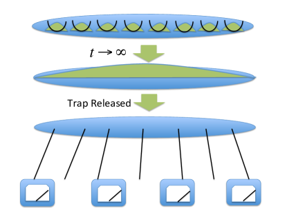
Figure 1: The Lieb Liniger gas is initialized in a nonequilibrium state - the Mott insulator (say by applying an external lattice). The lattice is removed and the system is allowed to relax for a long time. Its correlation functions are then measured.

In this work we consider the repulsive Lieb-Liniger model. We consider the case when the system is initialized in a deep lattice. So the state of the system is well described by a Mott insulator:

$$\left|\Phi_{0}\right\rangle=\prod_{j=-\infty}^{\infty}\int_{-\infty}^{\infty}\varphi\left(x+jl\right)b^{\dagger}\left(x\right)\left|0\right\rangle$$ (3)

with $\varphi\left(x\right)=\frac{e^{-x^{2}/\sigma}}{\left(\pi\sigma/2\right)^{1/4}}$, with $\sqrt{\sigma}\ll l$. The lattice is then released so that the system evolves under the Hamiltonian given in Eq. (1). The Lieb-Liniger gas is allowed to relax for a long time, $\left|\Psi\right\rangle=e^{iH_{LL}t}\left|\Phi_{0}\right\rangle$, thereby establishing a GGE with $\rho_{GGE}\cong\left|\Psi\right\rangle\left\langle\Psi\right|$, see figure (1). We note that using a saddle point approach the authors in key-1-1 (21) were able to identify the limit value $\left|\Psi\right\rangle\left\langle\Psi\right|$ with $\left|\vec{k}_{0}\right\rangle\left\langle\vec{k}_{0}\right|$, where the quasiparticle distribution characterizing $\vec{k}_{0}$ satisfies the appropriate Bethe-Ansatz equation (see below).

In this work we establish the exact quasiparticle density of this GGE. We use it to calculate various correlation functions for the final state. In particular we find a Gaussian decay of the density density correlation function at large distances for the final state. Overall we obtain a complete characterization of the final state. Our results are applicable for any coupling constant $c>0$. We would like to note that a quench between a BEC and a Lieb-Liniger gas has been previously considered in key-3-1 (22). The rest of the paper is organized as follows. In Section II we calculate the quasiparticle density of the final state; in Section III we compute the two and three body local correlation functions for the final state; in Section IV we compute the long distance density density correlation functions of the final state, here we also generalize our results (we see that the final correlation functions are heavily independent of certain types of disorder) and in Section V we conclude.

II Quasiparticle density

We would like to characterize the final state obtained in the quench between a Mott insulator and the Lieb-Liniger gas, it is given by a GGE. For the Lieb-Liniger gas it is possible to reduce the GGE density matrix to a pure state key-1-1 (21). That is for any local correlation function $\Theta$:

$$tr\left[\Theta\rho_{GGE}\right]=\left\langle\vec{k}_{0}\right|\Theta\left|\vec{k}_{0}\right\rangle$$ (4)

for an appropriately chosen eigenstate of the Lieb Liniger Hamiltonian $\left|\vec{k}_{0}\right\rangle$. Furthermore following the authors of key-1-1 (21) we are able to specify this pure state $\left|\vec{k}_{0}\right\rangle$. To do so let us denote by $L\rho_{p}\left(k\right)dk$ as the number of particles in the interval $\left[k,k+dk\right]$, $L\rho_{h}\left(k\right)dk$ as the number of holes in the interval $\left[k,k+dk\right]$ and $L\rho_{t}\left(k\right)dk$ as the number of states in the interval $\left[k,k+dk\right]$ so that $\rho_{t}\left(k\right)=\rho_{p}\left(k\right)+\rho_{h}\left(k\right)$. Here $L$ is the length of the system. Then the density of particles in k-space corresponding to $\left|\vec{k}_{0}\right\rangle$ is given by the following equations key-1-1 (21):

$$L\int dk\rho_{p}\left(k\right)k^{n}=I_{n}\left(t=0\right).$$ (5)

Therefore to characterize the density of quasiparticles of the final sate one needs to compute the various conserved quantities $I_{n}\left(t=0\right)$. To do so note that the conserved charges $I_{n}$ are given by integrals of local densities:

$$I_{n}=\int dxJ_{n}\left(x\right)$$ (6)

with the local densities being given by $J_{0}\left(x\right)=b^{\dagger}\left(x\right)b\left(x\right)$, $J_{1}\left(x\right)=ib^{\dagger}\left(x\right)\partial_{x}b\left(x\right)$, $J_{2}\left(x\right)=\partial_{x}b^{\dagger}\left(x\right)\partial_{x}b\left(x\right)+c\left(b^{\dagger}\left(x\right)b\left(x\right)\right)^{2}$, $J_{3}\left(x\right)=b^{\dagger}\left(x\right)\partial_{x^{3}}^{3}b\left(x\right)-\frac{3c}{2}\left(b^{\dagger}\left(x\right)\right)^{2}\partial_{x}\left(b\left(x\right)\right)^{2}$ etc. Since these changes are local and the wave function in Equation (3) is given by a sum of local non-overlapping single particle terms we have that:

$$I_{n}\left(t=0\right)=\frac{L}{l}\left\langle 0\right|\int dx\varphi\left(x\right)b\left(x\right)I_{n}\int dy\varphi\left(y\right)b^{\dagger}\left(y\right)\left|0\right\rangle$$ (7)

However for a single particle state it is straightforward to calculate the value of a local conserved quantity; indeed $I_{n}\left|k\right\rangle=k^{n}\left|k\right\rangle$. From this we obtain that the conserved charges are zero for odd $n$ and for even $n$ they are given by:

$$I_{n}\left(t=0\right)=\frac{L}{l}\,\left(\frac{2}{\sigma}\right)^{\frac{n}{2}}\,\frac{n!}{2^{\frac{n}{2}}\left(\frac{n}{2}!\right)}$$ (8)

In particular these are finite key-3-1 (22). Therefore according to Equation (5) the quasiparticle density $\rho_{p}\left(k\right)$ is a distribution whose moments are given by Equation (8). However it is straightforward to obtain such a distribution it is given by:

$$\rho_{p}\left(k\right)=\frac{\sigma^{\frac{1}{2}}}{\pi^{\frac{1}{2}}l}\exp\left(-\frac{k^{2}\sigma}{2}\right)$$ (9)

We note that this expression is completely independent of the coupling constant $c$ and works for all $c>0$. This distribution completely characterizes all the properties of the final state and completely determines $\rho_{GGE}$. For future use we would like to compute the total density of available states $\rho_{t}\left(k\right)$ as well as the ratio $\frac{\rho_{p}\left(k\right)}{\rho_{t}\left(k\right)}$. The total quasiparticle density is given by the equation key-31 (23):

$$\rho_{t}\left(k\right)=\frac{1}{2\pi}+\frac{1}{2\pi}\int dqK\left(k,q\right)\rho_{p}\left(q\right),$$ (10)

here $K\left(k,q\right)=\frac{2c}{c^{2}+\left(k-q\right)^{2}}$. We note that for $l\gg\sqrt{\sigma}$ $\rho_{t}\left(k\right)\cong\frac{1}{2\pi}$. Furthermore the occupation probability is given by $f\left(k\right)\equiv\frac{\rho_{p}\left(k\right)}{\rho_{t}\left(k\right)}\cong\frac{2\sqrt{\pi\sigma}}{l}\exp\left(-\frac{k^{2}\sigma}{2}\right)$. We note that the charges $I_{n}\left(t=0\right)$ grow very rapidly so are high order charges are important as such the results presented in key-20-1 (24) about exponential decay of density density correlations will not apply as we will see in Eq. (20).

III Local correlation functions

We would like to calculate the local correlation functions $\langle b^{\dagger}\left(0\right)b\left(0\right)\rangle$, $\langle b^{\dagger}\left(0\right)b^{\dagger}\left(0\right)b\left(0\right)b\left(0\right)\rangle$ and $\langle b^{\dagger}\left(0\right)b^{\dagger}\left(0\right)b^{\dagger}\left(0\right)b\left(0\right)b\left(0\right)b\left(0\right)\rangle$. The first of these quantities measures the density of particles in the system the second measures the effect of interactions while the third measure the the three particle recombination rate. From conservation of particle number the density of particles is given in the long time limit by $\rho=\langle b^{\dagger}\left(0\right)b\left(0\right)\rangle=\frac{1}{l}$. The two body correlation function is given by key-20 (25):

$$\begin{array}[t]{l}\left\langle b^{\dagger}\left(0\right)b^{\dagger}\left(0\right)b\left(0\right)b\left(0\right)\right\rangle\cong\\ \cong 2\int\frac{dk_{1}}{2\pi}\int\frac{dk_{2}}{2\pi}f\left(k_{1}\right)f\left(k_{2}\right)\frac{\left(k_{2}-k_{1}\right)^{2}}{\left(k_{2}-k_{1}\right)^{2}+c^{2}}+.....\end{array}$$ (11)

This integral may be done explicitly:

$$\left\langle b^{\dagger}\left(0\right)b^{\dagger}\left(0\right)b\left(0\right)b\left(0\right)\right\rangle =\frac{2}{l^{2}}-\frac{2\sqrt{\pi c^{2}\sigma}}{l^{2}}\times$$

$$\times\left[\exp\left(\frac{\sigma c^{2}}{4}\right)Erfc\left(\sqrt{\frac{\sigma c^{2}}{4}}\right)\right]$$ (12)

The three body integrals may be done similarly key-20 (25). They are given by:

$$\begin{array}[t]{l}\left\langle b^{\dagger}\left(0\right)b^{\dagger}\left(0\right)b^{\dagger}\left(0\right)b\left(0\right)b\left(0\right)b\left(0\right)\right\rangle\cong\\ \cong 6\int dk_{1}dk_{2}dk_{3}f\left(k_{1}\right)f\left(k_{2}\right)f\left(k_{3}\right)\times\\ \qquad\times\frac{\left(k_{2}-k_{1}\right)^{2}}{\left(k_{2}-k_{1}\right)^{2}+c^{2}}\frac{\left(k_{3}-k_{1}\right)^{2}}{\left(k_{3}-k_{1}\right)^{2}+c^{2}}\frac{\left(k_{3}-k_{2}\right)^{2}}{\left(k_{3}-k_{2}\right)^{2}+c^{2}}+....\end{array}$$ (13)

rSimplifying we can evaluate this expression in various limits. In the case that $\sigma c^{2}\ll 1$ we obtain that

$$\left\langle b^{\dagger}\left(0\right)b^{\dagger}\left(0\right)b^{\dagger}\left(0\right)b\left(0\right)b\left(0\right)b\left(0\right)\right\rangle\cong\frac{6}{l^{3}}$$ (14)

In the case that $\sigma c^{2}\gg 1$ we obtain that:

$$\left\langle b^{\dagger}\left(0\right)b^{\dagger}\left(0\right)b^{\dagger}\left(0\right)b\left(0\right)b\left(0\right)b\left(0\right)\right\rangle\cong\frac{9\times 2^{\frac{9}{2}}}{l^{3}c^{6}\sigma^{3}}$$ (15)

As such we see a strong suppression of the three body decay rates for large coupling constants $c$.

IV Density Density correlations

The density density correlation function for generic states has been previously calculated. We can use this to find the density density correlation function for our GGE. It is given by key-21 (26):

$$\left\langle\rho\left(x\right)\rho\left(0\right)\right\rangle=\rho^{2}+\sum_{k=2}^{\infty}\Gamma_{k}\left(x\right)$$ (16)

with the dominant term being given by key-21 (26):

$$\Gamma_{2}\left(x\right)= -\frac{1}{4\pi^{2}}\int_{-\infty}^{\infty}dk_{1}\omega\left(k_{1}\right)f\left(k_{1}\right)\int_{-\infty}^{\infty}dk_{2}\omega\left(k_{2}\right)f\left(k_{2}\right)\times$$

$$\times\left(\frac{k_{1}-k_{2}+ic}{k_{1}-k_{2}-ic}\right)\left[\frac{p\left(k_{1},k_{2}\right)}{k_{1}-k_{2}}\right]^{2}\exp\left(xp\left(k_{1},k_{2}\right)\right)$$ (17)

Here $\omega\left(k\right)=\exp\left(-\frac{1}{2\pi}\int_{-\infty}^{\infty}K\left(k,q\right)f\left(q\right)dq\right)$ and the function $p\left(k_{1},k_{2}\right)$ is given by:

$$p\left(k_{1},k_{2}\right)=-i\left(k_{1}-k_{2}\right)+\int_{-\infty}^{\infty}dt\,f\left(t\right)\,P\left(t,k_{1},k_{2}\right)$$ (18)

The function $P\left(t,k_{1},k_{2}\right)$ is defined through the following integral equation:

$$1+2\pi\,P\left(t,k_{1},k_{2}\right) =\left(\frac{k_{1}-t+ic}{k_{1}-t-ic}\right)\left(\frac{k_{2}-t-ic}{k_{2}-t+ic}\right)\times$$

$$\times\exp\left(\int K\left(t,s\right)f\left(s\right)P\left(s,k_{1},k_{2}\right)\right).$$ (19)

In the case when $l\gg\sqrt{\sigma}$ these equations greatly simplify. Indeed in that case $\omega\left(k\right)\cong e^{-1}$ and $p\left(k_{1},k_{2}\right)=-i\left(k_{1}-k_{2}\right)$. With these simplifications the integral in Eq. (17) becomes,

$$\left\langle\rho\left(x\right)\rho\left(0\right)\right\rangle\cong\rho^{2}+\frac{1}{4\pi^{2}e^{2}l^{2}}\exp\left(-\frac{x^{2}}{\sigma}\right)$$ (20)

We see a gaussian decay of correlation functions at large distances.

We would like to note that the final result e.g. the final quasiparticle density see Eq. (9) is independent of positional disorder in the Mott insulator. Indeed if the centers of the particles in the Mott insulator do not form a uniform lattice but instead have random locations (which would happen for example for a partial filling of the first Mott band) none of the conserved quantities, see Equation (8), change. In particular if the particles have an average interparticle separation $\bar{l}$ then the final state has exactly the same correlations as those given in the main text except with $l\rightarrow\bar{l}$ see Equations (12), (14), (15) and (20). As such we can characterize these states as well.

V Conclusions

We have studied a quench between a Mott insulator and a Lieb-Liniger liquid. We have found that at long time the system equilibrates to a GGE. We have characterized the GGE quasiparticle density exactly and found it to be gaussian. We were able to compute local two and three body correlation functions as well as density density correlations. We have found the density density correlation to decay in a Gaussian manner with distance. We argued our results to be robust to certain kinds of disorder. The methods used in this paper open the possibility to compute the final state after a quench when the initial state is given by a collection of isolated few body states (such as a collection of dimer molecules on a lattice). The conserved quantities can be calculated in that case as well allowing us to obtain the final quasiparticle density as well as various correlation functions.

The results presented here have direct experimental applicability. Indeed it is not too difficult to prepare a gas of bosons in the Mott insulator state key-21-1 (27). The three body density density correlations may be measured through trap loss rates key-20 (25) or through the third moment of the number of particles key-22 (28). The density density correlators studied may be measured through time of flight interferometry key-21-1 (27), all directly experimentally relevant.

Acknowledgments: This research was supported by NSF grant DMR 1006684 and Rutgers CMT fellowship.

References

- (1) T. Kinoshita, T. Wenger, and D. S. Weiss, Nature (London) 440, 900 (2006)
- (2) M. Greiner, O. Mandel, T. W. Hansch and I. Bloch, Nature 419, 51, (2002).
- (3) S. Hofferberth, I. Lesanovsky, B. Fischer, T. Schumm and J. Schniedmayer, Nature 449, 324 (2007).
- (4) E. Haller, M. Gusatvsson, M. J. Mark, J. G. Danzl, R. Hart, G. Pupillo and H.-C. Nagerl, Science 325, 1224 (2009).
- (5) S. Trotsky, Y.-A. Chen, A. Flesch, I. P. McCulloch, U. Schollwock, J. Eisert and I. Bloch, Nature Phys. 8, 325 (2012).
- (6) M. Cheneau, P. Barmettler, D. Poletti, M. Endres, P. Schauss, T. Fukuhara, C. Gross, I Bloch, C. Kollath and S. Kuhr, Nature 481, 484 (2012).
- (7) M. Gring, M. Kuhnert, T. Langen, T. Kitagawa, B. Rauer, M. Schreitl, I. Mazets, D. A. Smith, E. Demler, and J. Schmiedmayer, Science 337, 1318 (2012).
- (8) U. Schneider, L. Hakermuller, J. P. Ronzheimer, S. Will, S. Braun, T. Best, I Bloch, E. Demler, S. Mandt, D. Rasch, and A. Rosch, Nature Phys. 8, 213 (2012).
- (9) J. P. Ronzheimer, M. Schreiber, S. Braun, S. S. Hodgman, S. Langer, I. P. McCulloch, F. Heidrich-Meisner, I. Bloch and U. Schneider, Phys. Rev. Lett. 110, 205301 (2013).
- (10) M. Rigol, V. Dunjko, and M. Olshanii, Nature 452, 854, (2008).
- (11) P. Calabrese and J. Cardy, Phys. Rev. Lett. 96, 136801 (2006).
- (12) M. Eckstein, M. Kollar, and P. Werner, Phys. Rev. Lett. 103, 056403 (2009).
- (13) A. Faribault, P. Calabrese and J. S. Caux J. Stat. Mech. P03018 (2009).
- (14) S. Sotiriadis, D. Fioretto, and G. Mussardo, J. Stat. Mech. P02017 (2012).
- (15) J. Mossel and J. S. Caux, J. Phys. A 45, 255001 (2012).
- (16) T. Barthel, and U. Schollwock, Phys. Rev. Lett. 100, 100601 (2008).
- (17) M. Rigol and M. Fitzpatrick, Phys. Rev. A 84, 033640 (2011).
- (18) M. Rigol, V. Dunjko, V. Yurovsky, and M. Olshanii, Phys. Rev. Lett. 98, 050405 (2007).
- (19) E. H. Lieb and W. Liniger, Phys. Rev. 130, 1605 (1963).
- (20) G. Goldstein and N. Andrei, arXiv 1309.7029
- (21) J. Mossel, J.-S. Caux, J. Phys. A: Math. Theor. 45, 255001, (2012).
- (22) M. Kormos, A. Shashi, Y.-Z. Chou, J.-S. Caux, Adilet Imambekov Phys. Rev. B 88, 205131 (2013).
- (23) M. Takahashi, Thermodynamics of one-dimensional solvable models, (Cambridge University Press, 1999).
- (24) G. Goldstein and N. Andrei, arXiv 1405.6365.
- (25) M. Kormos, G. Mussardo and A. Tronbettini, Phys. Rev. A 81, 043606 (2010).
- (26) N. M. Bogoliubov and V. E. Korepin, Nuclear physics B257, 766 (1985).
- (27) I. Bloch, J. Dalibard, and W. Zwerger, Rev. Mod. Phys. 80, 885 (2008).
- (28) J. Armijo, T. Jacqmin, K. V. Kheruntsyan, and I. Bouchoule, Phys. Rev. Lett. 105, 230402 (2010).