Ising quantum Hall ferromagnetism in Landau levels $\left|N\right|\geq 1$ of bilayer graphene

Abstract

A magnetic field applied perpendicularly to the chiral two-dimensional electron gas (C2DEG) in a Bernal-stacked bilayer graphene quantizes the kinetic energy into a discrete set of Landau levels $N=0,\pm 1,\pm 2,...$While Landau level $N=0$ is eighfold degenerate, higher Landau levels ($\left|N\right|\geq 1$) are fourfold degenerate when counting spin and valley degrees of freedom. In this work, the Hartree-Fock approximation is used to study the phase diagram of the C2DEG at integer fillings $\widetilde{\nu}=1,2,3$ of these higher Landau levels. At these filling factors, the C2DEG is a valley or spin Ising quantum Hall ferromagnet. At odd fillings, the C2DEG is spin polarized and has all its electrons in one valley or the other. There is no intervalley coherence in contrast with most of the the ground states in Landau level $N=0.$ At even filling, $\widetilde{\nu}=2,$ the C2DEG is either fully spin polarized with electrons occupying both valleys or spin unpolarized with electron occupying one of the two valleys. A finite electric field (or bias) applied perpendicularly to the plane of the C2DEG induces a series of first-order phase transitions between these different ground states. The transport gap or its slope is discontinuous at the bias where a transition occurs. Such discontinuity may result in a change in the transport properties of the C2DEG at that bias.

I INTRODUCTION

In a strong perpendicular magnetic field $\mathbf{B}$, the kinetic energy of a two-dimensional electron gas (2DEG) is quantized into a series of discrete Landau levels with a macroscopic degeneracy $N_{\varphi}=SB/\Phi_{0},$ where $S$ is the sample area and $\Phi_{0}$ is the magnetic flux quantum. This quantization leads to the integer quantum Hall effect which has been the subject of intense study over the past $35$ yearsReview1 ; Review2 . The ground state of the 2DEG at odd values of the filling factors $\nu=N_{e}/N_{\varphi}$ (where $N_{e}$ is the number of electrons added to the 2DEG at the neutrality point) is completely spin polarized even when the Zeeman coupling is set to zero because a parallel orientation of the spins minimizes the Coulomb repulsion. This ground state is referred to as a spin quantum Hall ferromagnet (spin-QHF). In the absence of Zeeman coupling, this state has a SU(2) symmetry in spin space.

In a double quantum well system (DQWS), each electron has an extra layer degree of freedom which can be associated with a layer pseudospin $P_{z}=\pm 1/2$. At filling factor $\nu=1$ and when the 2DEG is spin polarized, the minimization of the capacitive energy of the 2DEG forces all electrons to be in a symmetric combination of the right and left layer in the ground state. The layer pseudospins are thus all aligned in the $xy-$plane in pseudospin space and the 2DEG is this time referred to as a layer-QHFKmoon . In the absence of tunneling between the two layers, the layer-QHF has a U(1) symmetry which is associated with the invariance of the ground state energy with respect to the orientation of the layer-pseudospin in the $xy-$plane. The physics of the layer-QHF is reviewed in Ref. Ezawa, .

Quantum Hall ferromagnetism can be associated with many other type of degrees of freedom. In graphene, for example, the ground state of the chiral 2DEG (C2DEG) at $1/4$ and $3/4$ fillings of the Landau levels $\left|N\right|\geq 1$ is a valley-QHF where the two pseudospin states are now associated with the non-equivalent valleys $K_{+}$ and $K_{-}.$ To a good approximation, the Coulomb interaction is independent of the valley indexGoerbig and since there is no symmetry-breaking term associated with the valley degree of freedom, the Hamiltonian has a SU(2) symmetry in valley-pseudospin space. Such is also the case in Landau level $N=0$ of a Bernal-stacked bilayer graphene (BLG), a system which has been extensively studied both theoretically and experimentally over the past few yearsBarlasRevue2012 . Because of its extra orbital degeneracy, the $N=0$ Landau level in BLG has an eightfold degeneracy in the absence of Zeeman coupling in the minimal tight-binding model where only the in-plane, $\gamma_{0},$ and inter-plane, $\gamma_{1},$ hopping terms are considered. In contrast with graphene, an electric field (or bias) applied perpendicularly to the plane of the layers in BLG breaks the valley degeneracy and also the layer degeneracy since valley and layer degrees of freedom are equivalent in $N=0$. Moreover, when Coulomb interaction is taken into account, a rich set of quantum Hall ferromagnets emerges at integer filling factors $\nu\in\left[-4,4\right]$ as the bias is variedLambert .

In this paper, the Hartree-Fock approximation (HFA) is used to study the quantum Hall ferromagnetic ground states of the C2DEG in a Bernal-stacked graphene bilayer in the higher Landau levels $\left|N\right|\geq 1.$ By contrast with $N=0,$ the higher Landau levels are fourfold degenerate in the absence of Zeeman coupling because there is no orbital degree of freedom in higher Landau levels. The QHF states are studied at integer fillings $\widetilde{\nu}=1,2,3$ of the Landau level $N\$and as a function of the magnetic field strength $B$ and the electrical bias $\Delta_{B}$. The behavior of the C2DEG in $\left|N\right|\geq 1$ is found to be very different than that in level $N=0.$ In the latter case, the ground states at zero bias, with the exception of $\nu=0,$ are valley-QHFs with a U(1) symmetry in the $xy-$plane. In the former case, the quantum Hall ferromagnetism is of the Ising type with two degenerate ground states at $\Delta_{B}=0$. No intervalley coherence is possible. At finite Zeeman coupling and in the absence of bias, the ground states at $\widetilde{\nu}=1,3$ are Ising valley-QHFs with a $Z_{2}$ symmetry in valley-pseudospin space. A finite bias $\Delta_{B}$ can induce a first order phase transition between the two pseudospin states. At filling $\widetilde{\nu}=2$ of level $N$, the C2DEG is a spin-QHF below a certain critical bias $\Delta_{B}^{\left(c\right)}$ that depends on the magnetic field and on the dielectric constant of the substrate. Above $\Delta_{B}^{\left(c\right)}$, the system is a valley-QHF with valley pseudospin $P_{z}=\pm 1.$ The phase diagram is found to depend sensitively on the Landau level index $N$ and on the value of the dielectric constant $\kappa.$ The transition between two QHF phases is accompanied by a discontinuity in the Hartree-Fock electron-hole gap (the transport gap) or its slope. Depending on the Landau level broadening due to disorder, this discontinuity may lead to a disappearance of the quantum Hall effect and to an increase in the longitudinal resistivity at the transition. Such an effect has been seen in a recent experimentTutuc on double bilayer graphene in Landau levels $N\leq 0$. We find that our numerical results for the behavior of $\Delta_{B}^{\left(c\right)}$ with magnetic field are in qualitative agreement with these experimental results .

There has been up to now very few studies of the phase diagram of the C2DEG in higher Landau levels of BLG. Wigner and Skyrme crystal states have been studied near integer filling factorsSakurai , but the Ising behavior reported in the present article has not been discussed before in this system. It has, however, been studied previously in many other systems. Usually, the Ising behavior occurs when any two different Landau levels simultaneously approach the chemical potential. At the crossing point, the nature of the ground state is sensitive to the microscopic character of the crossing Landau levels and different types of QHF can occur. At even integer filling factor, the crossing often gives rise to a first-order paramagnetic to ferromagnetic transitionQuinn ; Daneshvar . A classification scheme that applies to single layer and bilayer semiconductor 2DEGs is presented in Ref. Classification, . In the present work, the Ising behavior can be related to the crossing of two sub-levels in a Landau level $N$ or be exchange-energy driven and not related to any Landau level crossings.

This paper is organized in the following way. Sections II, III and IV present the tight-binding model of BLG, the Hartree-Fock approximation for the Coulomb interaction and the Green’s function method used to calculate the order parameters of the different phases. Section V presents the pseudospin language used to describe the various phases. The phase diagrams for different filling factors are presented in Secs. VI,VII,VIII for $\widetilde{\nu}=1,3,2$ respectively. Section IX contains a discussion of our results and a comparison with the available experimental data.

II NON-INTERACTING HAMILTONIAN IN LANDAU LEVELS $N\geq 1$

The system considered in this paper is a Bernal-stacked graphene bilayer in a transverse magnetic $\mathbf{B=}B\widehat{\mathbf{z}}$ and electric field $\mathbf{E.}$ The electric field induces a potential difference (hereafter called the bias) $\Delta_{B}=Ed$ between the two layers, where $d=3.337$ Å is the interlayer separation. The crystal structure of each graphene layer is a honeycomb lattice that can be described as a triangular Bravais lattice with a basis of two carbon atoms $A_{n}$ and $B_{n},$ where $n=1,2$ is the layer index. The triangular lattice constant $a_{0}=2.\,\allowbreak 46$ Å $=\sqrt{3}c,$ where $c=1.42$ Å is the distance between two adjacent carbon atoms. The Brillouin zone of the reciprocal lattice is hexagonal and has two nonequivalent valley points $K_{\xi}=\left(\frac{2\pi}{a_{0}}\right)\left(\xi\frac{2}{3},0\right),$ where $\xi=\pm$ $1$ is the valley indexReviewGraphene .

In the absence of magnetic field and bias, the electronic band structure consists of four bands. The two middle bands meet at the six valley points while the two high-energy bands are separated by a gap $\gamma_{1}$ from the two middle, low-energy bands (see, for example, Fig. 1 of Ref. Manuel, ). In a finite magnetic field, each band is split into a set of Landau levels. Below, we use the index $j=1,2,3,4$ to refer to the set of Landau levels that originate from each band. The bands are indexed in order of increasing energy.

In the continuum approximation, the tight-binding Hamiltonian for $\mathbf{B}=0$ is expanded to linear order in the wave vector $\mathbf{p}=\mathbf{k}-\mathbf{K}_{\pm}$ in each valley. The effect of a magnetic field is taken into account by making the Peierls substitution $\mathbf{p}\rightarrow\mathbf{P}=\mathbf{p}+e\mathbf{A}/\hslash c$ (with $e>0$ for an electron) for the wave vector where $\mathbf{A}=\left(0,Bx,0\right)$ is the vector potential in the Landau gauge. The tight-binding Hamiltonian in the basis $\left\{A_{1},B_{1},A_{2},B_{2}\right\}$ for valley $K_{-}$ and $\left\{B_{2},A_{2},B_{1},A_{1}\right\}$ for valley $K_{+}$ is given by

$$H_{\xi}^{\left(0\right)}=\left(\begin{array}[]{cccc}\delta_{0}-\xi\frac{\Delta_{B}}{2}&\xi\alpha_{0}a&\xi\alpha_{4}a^{{\dagger}}&-\gamma_{1}\\ \xi\alpha_{0}a^{{\dagger}}&-\xi\frac{\Delta_{B}}{2}&\xi\alpha_{3}a&\xi\alpha_{4}a^{{\dagger}}\\ \xi\alpha_{4}a&\xi\alpha_{3}a^{{\dagger}}&\xi\frac{\Delta_{B}}{2}&\xi\alpha_{0}a\\ -\gamma_{1}&\xi\alpha_{4}a&\xi\alpha_{0}a^{{\dagger}}&\delta_{0}+\xi\frac{\Delta_{B}}{2}\end{array}\right),$$ (1)

where the parameter

$$\alpha_{i}=\sqrt{\frac{3}{2}}\frac{a_{0}}{\ell}\gamma_{i},$$ (2)

with $\ell=\sqrt{\hslash c/eB}$ the magnetic length. The hopping parameters in $H_{\xi}^{\left(0\right)}$are: $\gamma_{0}$ the in-plane nearest-neighbor (NN) hopping; $\gamma_{1}$ the interlayer hopping between carbon atoms that are immediately above one another (i.e. $A_{1}-B_{2}$); $\gamma_{3}$ the interlayer NN hopping term between carbon atoms of different sublattices (i.e. $A_{2}-B_{1}$) and $\gamma_{4}$ the interlayer next NN hopping term between carbons atoms in the same sublattice (i.e. $A_{1}-A_{2}$ and $B_{1}-B_{2}$). The parameter $\delta_{0}$ represents the difference in the crystal field between sites $A_{1},B_{2}$ and $A_{2},B_{1}$ and $\Delta_{B}$ is the potential difference between the two layers. For all calculations done in this paper, we use for the value of each parameterValues : $\gamma_{0}=3.12$ eV, $\gamma_{1}=0.39$ eV, $\gamma_{3}=0.29,$ $\gamma_{4}=0.12$ eV and $\delta_{0}=0.0156$ eV. The ladder operators $a,a^{{\dagger}}$ are defined such that $a\varphi_{n}\left(x\right)=-i\sqrt{n}\varphi_{n-1}\left(x\right)$ and $a^{{\dagger}}\varphi_{n}\left(x\right)=i\sqrt{n+1}\varphi_{n+1}\left(x\right),$ where $\varphi_{n}\left(x\right)$ with $n=0,1,2,...$ are the eigenfunctions of the one-dimensional harmonic oscillator that enter in the definition of the Landau-gauge wave functions

$$h_{n,X}\left(\mathbf{r}\right)=\frac{1}{\sqrt{L_{y}}}e^{-iXy/\ell^{2}}\varphi_{n}\left(x-X\right),$$ (3)

where $X$ is the guiding-center quantum number.

When the warping term $\gamma_{3}=0,$ the eigenspinors of $H_{\xi}^{\left(0\right)}$ in the basis $\left\{A_{1},B_{1},A_{2},B_{2}\right\}$ for both $K_{+}$ and $K_{-}$ have the form

$$\psi_{\xi=-1,n,j,X}^{\left(0\right)}\left(\mathbf{u}\right)=\left(\begin{array}[]{c}c_{-,n,j,1}h_{n-1,X}\left(\mathbf{r}\right)\chi_{1}\left(z\right)\\ c_{-,n,j,2}h_{n,X}\left(\mathbf{r}\right)\chi_{1}\left(z\right)\\ c_{-,n,j,3}h_{n-2,X}\left(\mathbf{r}\right)\chi_{2}\left(z\right)\\ c_{-,n,j,4}h_{n-1,X}\left(\mathbf{r}\right)\chi_{2}\left(z\right)\end{array}\right),$$ (4)

and

$$\psi_{\xi=+1,n,j,X}^{\left(0\right)}\left(\mathbf{u}\right)=\left(\begin{array}[]{c}c_{+,n,j,4}h_{n-1,X}\left(\mathbf{r}\right)\chi_{1}\left(z\right)\\ c_{+,n,j,3}h_{n-2,X}\left(\mathbf{r}\right)\chi_{1}\left(z\right)\\ c_{+,n,j,2}h_{n,X}\left(\mathbf{r}\right)\chi_{2}\left(z\right)\\ c_{+,n,j,1}h_{n-1,X}\left(\mathbf{r}\right)\chi_{2}\left(z\right)\end{array}\right),$$ (5)

where it is understood that $h_{n,X}\left(\mathbf{r}\right)=0$ if $n<0$ and the function $\left|\chi_{i}\left(z\right)\right|^{2}=\delta\left(z-z_{i}\right),$ where $z_{i}$ with $i=1,2$ is the position of layer $i$ along the $z$ axis and $\left|z_{2}-z_{1}\right|=d$. The three-dimensional vector $\mathbf{u}=\left(\mathbf{r},z\right),$ where $\mathbf{r}$ is a two-dimensional vector in the plane of the bilayer. The corresponding energy levels are written as $E_{\xi,n,j}^{\left(0\right)}.$ They are independent of $X$ and so they have degeneracy $N_{\varphi}=S/2\pi\ell^{2},$ where $S$ is the 2DEG area. As Fig. 1 shows, for $n=0$ there is one eigenspinor that belongs to the Landau levels of band $j=2$ for $K_{+}$ or $j=3$ for $K_{-}$. For $n=1,$ there are three eigenspinors belonging to bands $j=1,2,4$ for $K_{+}$ and to $j=1,3,4$ for $K_{-}$. The solutions $n=0,j=2$ or $3$ and $n=1,j=2$ or $3$ are degenerate when $\Delta_{B},\gamma_{4},\delta_{0}=0$ and are considered as belonging to Landau level $N=0$ which has thus an eightfold degeneracy when counting spin and valley degrees of freedom. This degeneracy is called the orbital degeneracy. For $n\geq 2,$ there are four energy eigenspinors, one for each energy band $j$. Hereafter, we only work with bands $2$ and $3$ and so we label the levels of band $j=2$ by $N=-1,-2,-3,...$ and those of band $j=3$ by $N=1,2,3,...$ as indicated in Fig. 1. All Landau levels $\left|N\right|>0$ are fourfold degenerate when spin and valley degrees of freedom are considered.

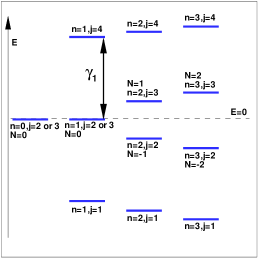
Figure 1: (Color online) Labeling of the energy levels for one valley and one spin component at zero bias and for $\gamma_{4}=\delta_{0}=0$. The vertical position of each line does not reflect the actual energy of each level.

The warping term $\gamma_{3}$ couples the eigenspinors together so that a solution of the full non-interacting Hamiltonian can be written as the linear combination

$$\widetilde{\psi}_{\xi,n,j,X}^{\left(0\right)}\left(\mathbf{u}\right)=\sum_{n^{\prime},j^{\prime}}b_{\xi,n^{\prime},j^{\prime}}^{\left(0\right)}\psi_{\xi,n^{\prime},j^{\prime},X}\left(\mathbf{u}\right)$$ (6)

with the normalization condition $\sum_{n,j}\left|b_{\xi,n,j}\right|^{2}=1$. In this paper, we are interested in the phase diagram of the 2DEG in Landau levels $\left|N\right|=1,2,3.$ In order to estimate the importance of the hopping term on these levels, we compare the energies $E_{\xi,n,j}^{\left(0\right)}$ and coefficients $b_{\xi,n,j}$ computed with or without it. The results are shown in Table 1 for the valley $\xi=+1$, band $j=3,$ and for different values of the magnetic field at zero bias. Clearly, for these levels, neglecting the warping term $\gamma_{3}$ is a good approximation. That is why, hereafter, we set $\gamma_{3}=0$ and use the simpler eigenspinors given by Eqs. (4),(5). We remark that we do not use the effective two-component modelMcCann in this paper since it is not good at describing the higher Landau levelsManuel .

$N$	$B$ (T)	$\gamma_{3}=0,E_{{}_{+,N+1,3}}^{\left(0\right)}$	$\gamma_{3}\neq 0,E_{{}_{+,N+1,3}}^{\left(0\right)}$	$\left|b_{+,N+1,3}\right|^{2}$
$1$	$10$	$0.04857$	$0.04821$	$0.988$
$2$	$10$	$0.07847$	$0.07845$	$0.975$
$3$	$10$	$0.105$	$0.105$	$0.970$
$1$	$40$	$0.153$	$0.153$	$0.995$
$2$	$40$	$0.232$	$0.232$	$0.989$
$3$	$40$	$0.298$	$0.297$	$0.983$

Table 1: Non-interacting energies and expansion coefficients calculated with and without the warping term for different values of the Landau level $N,j=3$ at magnetic fields $B=10$ T and $40$ T in the valley $K_{+}$.

Figure 2 (a) shows the energy of the Landau levels $N=0,1,2$ as a function of the bias $\Delta_{B}$ for $B=10$ T. The identification of the levels is made in Fig. 2 (b). For Landau level $N=0,$ the levels shown are those corresponding to $n=0,1$ (of both spins) in valley $K_{-}.$ By contrast, the energy of levels $n=0,1$ in valley $K_{+}$ (not shown) decreases with bias. It is important to notice that, in Landau level $N=0,$ valley and layer indices are equivalent (in the two-component model) but not this is not true in higher Landau levels as can easily be seen from the eigenspinors in Eqs. (4),(5).

Crossings between different Landau levels occur for $\Delta_{B}\gtrsim 0.14$ eV. This value sets an upper limit to our numerical calculation since we will neglect Landau level mixing. In this work, we will thus restrict our calculation to $\left|\Delta_{B}\right|\leq 0.1$ eV, a bias that corresponds to an interlayer electric field of $E\approx 0.3$ V/nm. Crossings between the non-interacting energy levels also occur within a given Landau level. An example is shown in Fig. 2 (b) where a crossing between $E_{+,N+1,3}^{(0)}$ with spin up and $E_{-,N+1,3}^{(0)}$ with spin down at $B=10$ T occurs at $\Delta_{B}=0.014$ eV for $N=1.$Such crossing is of course taken into account.

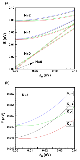
Figure 2: (Color online) (a) Dispersion of the Landau levels $N=0,1,2$ with bias $\Delta_{B}$ for $B=10$ T; (b) part of the same energy spectrum for level $N=1$ showing the crossing between the sub-levels $(K_{+},+)$ and $(K_{-},-).$

Defining $\nu_{\pm}$ as the filling factors for valleys $K_{\pm}$ and $\nu_{1,2}$ as the filling factors for layers $1$ and $2,$ we have for each level (we now omit the indices $N,j$ to simplify the notation)

$$\nu_{1} = n_{1,+}\nu_{+}+n_{1,-}\nu_{-},$$ (7)

$$\nu_{2} = n_{2,+}\nu_{+}+n_{2,-}\nu_{-},$$ (8)

where the projectors

$$n_{1,+} = \left|c_{+,4}\right|^{2}+\left|c_{+,3}\right|^{2},$$ (9)

$$n_{1,-} = \left|c_{-,1}\right|^{2}+\left|c_{-,2}\right|^{2},$$ (10)

$$n_{2,+} = \left|c_{+,1}\right|^{2}+\left|c_{+,2}\right|^{2},$$ (11)

$$n_{2,-} = \left|c_{-,3}\right|^{2}+\left|c_{-,4}\right|^{2}.$$ (12)

Obviously,

$$n_{1} = n_{1,+}+n_{1,-},$$ (13)

$$n_{2} = n_{2,+}+n_{2,-},$$ (14)

and from the normalization condition $\sum_{i=1}^{i=4}\left|c_{\xi,n,j,i}^{2}\right|=1$ for the eigenspinors

$$n_{1,\pm}+n_{2,\pm}=1.$$ (15)

The eigenspinor coefficients are related by

$$c_{+,j}\left(\Delta_{B}\right)=\left[c_{-,j}\left(-\Delta_{B}\right)\right]^{\ast}$$ (16)

so that at zero bias

$$n_{1,\mp}=n_{2,\pm}.$$ (17)

Figure 3 shows the coefficients $\left|c_{\xi,i}\right|^{2}$ and the projectors $n_{1,\pm},n_{2,\pm},n_{1},n_{2}$ as a function of bias for $B=10$ T and $N=1.$ For a positive bias, layer $1$ has a higher energy than layer $2$ and Eq. (1) gives $c_{+,1},c_{+,2},c_{-,3},c_{-,4}\rightarrow 0$ at large positive bias so that the electrons occupy layer 1 in this limit. This is consistent with the fact that Landau levels $N>0,$ which correspond to antibonding states of the layers, have higher energies than Landau levels $N<0$ which are bonding states.

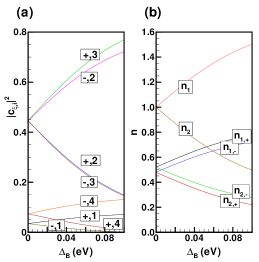
Figure 3: (Color online) (a) Coefficients $\left|c_{\xi,i}\right|^{2}$ and (b) projectors $n_{1,\pm},n_{2,\pm},n_{1},n_{2}$ as a function of bias for $B=10$ T and Landau level $N=1$.

III HARTREE-FOCK HAMILTONIAN

We now project the Hamiltonian into Landau level $N$ (with $N>0$ standing for $N,j=3$ and $N<0$ standing for $N,j=2$). The Coulomb interaction in this level is given by

$$V_{C} = \frac{1}{2}\sum\limits_{\xi,\xi^{\prime},\sigma,\sigma^{\prime}}\int d\mathbf{u}\int d\mathbf{u}^{\prime}\Psi_{N,\xi,\sigma}^{{\dagger}}\left(\mathbf{u}\right)$$

$$\times\Psi_{N,\xi^{\prime},\sigma^{\prime}}^{{\dagger}}\left(\mathbf{u}^{\prime}\right)V\left(\mathbf{u}-\mathbf{u}^{\prime}\right)\Psi_{N,\xi^{\prime},\sigma^{\prime}}\left(\mathbf{u}^{\prime}\right)\Psi_{N,\xi,\sigma}\left(\mathbf{u}\right),$$

where terms that do not conserve the valley index have been neglectedGoerbig . The field operator $\Psi_{N,\xi,\sigma}$ is defined by

$$\Psi_{N,\xi,\sigma}\left(\mathbf{u}\right)=\sum_{X}\psi_{\left|N\right|+1,\xi,X}^{\left(0\right)}\left(\mathbf{u}\right)c_{N,\xi,X,\sigma},$$ (19)

where $c_{N,\xi,X,\sigma}$ annihilates an electron with quantum numbers $\xi,N,\sigma$ where $\sigma=\pm 1$ is the spin index. The Coulomb potential $V\left(\mathbf{u}-\mathbf{u}^{\prime}\right)$ is given by

$$V\left(\mathbf{u}-\mathbf{u}^{\prime}\right)=\frac{1}{S}\sum_{\mathbf{q}}\frac{2\pi e^{2}}{\kappa q}e^{i\mathbf{q}\cdot\left(\mathbf{r}-\mathbf{r}^{\prime}\right)}e^{-q\left|z-z^{\prime}\right|},$$ (20)

where $\kappa$ is the dielectric constant of the substrate. When there is no ambiguity, we will drop the index $N$ to simplify the notation.

We define the operator

$$\rho_{\xi,\xi^{\prime}}^{\sigma,\sigma^{\prime}}\equiv\frac{1}{N_{\varphi}}\sum_{X}c_{\xi,X,\sigma}^{\dagger}c_{\xi^{\prime},X,\sigma^{\prime}}$$ (21)

so that the set of average values $\left\{\left\langle\rho_{\xi,\xi^{\prime}}^{\sigma,\sigma^{\prime}}\right\rangle\right\}$ can serve as the order parameters of any uniform state of the C2DEG. The non uniform states can be described by a space dependent analog of $\left\langle\rho_{\xi,\xi^{\prime}}^{\sigma,\sigma^{\prime}}\right\rangle$Lambert . In this work, however, we consider only the uniform states.

The Hartree-Fock Hamiltonian $H_{HF}$ is obtained by making the Hartree and Fock pairings of the field operators in $V_{C}$. The diverging part of the Hartree interaction is cancelled by considering the interaction of the electrons with the neutralizing positive background and so

$$H_{HF} = -N_{\varphi}\alpha_{d}\frac{\widetilde{\nu}^{2}}{4}$$

$$+N_{\varphi}\sum_{\xi,\sigma}\left(\frac{\widetilde{\nu}}{2}\alpha_{d}+E_{\xi,\sigma}\right)\rho_{\xi,\xi}^{\sigma,\sigma}$$

$$-N_{\varphi}\sum_{\xi,\zeta,\sigma,\sigma^{\prime}}X^{\left(\xi,\zeta\right)}\left\langle\rho_{\xi,\zeta}^{\sigma,\sigma^{\prime}}\right\rangle\rho_{\zeta,\xi}^{\sigma^{\prime},\sigma},$$

where $\widetilde{\nu}$ is the filling factor of Landau level $N$ and we have defined the constant

$$\alpha_{d}=\frac{d}{\ell}\left(\frac{e^{2}}{\kappa\ell}\right)$$ (23)

as well as the renormalized single-particle energy $E_{\xi,\sigma}$

$$E_{\xi,\sigma} = E_{\xi}^{\left(0\right)}-\frac{1}{2}\sigma\Delta_{Z}$$

$$+\sum_{\zeta,\sigma^{\prime}}A^{\left(\xi,\zeta\right)}\left\langle\rho_{\zeta,\zeta}^{\sigma^{\prime},\sigma^{\prime}}\right\rangle,$$

where $A_{N}^{\left(\xi,\zeta\right)}$ is the non-diverging part of the Hartree interaction $H^{\left(\xi,\zeta\right)}\left(0\right)$ (see below) i.e.

$$A^{\left(+,+\right)} = -2\alpha_{d}n_{2,+}n_{1,+},$$ (25)

$$A^{\left(+,-\right)} = A^{\left(-,+\right)}=-\alpha_{d}\left(n_{2,+}n_{1,-}+n_{1,+}n_{2,-}\right),$$ (26)

$$A^{\left(-,-\right)} = -2\alpha_{d}n_{1,-}n_{2,-}.$$ (27)

In graphene, the Zeeman coupling $\Delta_{Z}=g\mu_{B}B=1.158\times 10^{-4}$ $B$ (T) eV.

The Hartree and Fock interactions are given by

$$H^{\left(\xi,\xi^{\prime}\right)}\left(x\right) = \left(\frac{e^{2}}{\kappa\ell}\right)\frac{V^{\left(\xi,\xi^{\prime}\right)}\left(x\right)}{x},$$ (28)

$$X^{\left(\xi,\xi^{\prime}\right)} = \left(\frac{e^{2}}{\kappa\ell}\right)\int_{0}^{\infty}dxV^{\left(\xi,\xi^{\prime}\right)}\left(x\right),$$ (29)

where

$$V^{\left(\xi,\xi\right)}\left(x\right)$$ (30)

$$=G_{1}^{\left(\xi\right)}\left(x\right)G_{1}^{\left(\xi\right)}\left(x\right)+G_{2}^{\left(\xi\right)}\left(x\right)G_{2}^{\left(\xi\right)}\left(x\right)$$

$$+2e^{-xd/\ell}G_{1}^{\left(\xi\right)}\left(x\right)G_{2}^{\left(\xi\right)}\left(x\right),$$

$$V^{\left(\xi,\overline{\xi}\right)}\left(x\right)$$

$$= G_{1}^{\left(\xi\right)}\left(x\right)G_{2}^{\left(\overline{\xi}\right)}\left(x\right)+G_{2}^{\left(\xi\right)}\left(x\right)G_{1}^{\left(\overline{\xi}\right)}\left(x\right)$$

$$+e^{-xd/\ell}\left[G_{1}^{\left(\xi\right)}\left(x\right)G_{1}^{\left(\overline{\xi}\right)}\left(x\right)+G_{2}^{\left(\xi\right)}\left(x\right)G_{2}^{\left(\overline{\xi}\right)}\left(x\right)\right],$$

where $\overline{\xi}=-\xi$ and the functions

$$G_{1}^{\left(\xi\right)}\left(x\right)$$

$$= e^{\frac{-x^{2}}{4}}\left[\left|c_{\xi,1}\right|^{2}L_{N-1}\left(\frac{x^{2}}{2}\right)+\left|c_{\xi,2}\right|^{2}L_{N}\left(\frac{x^{2}}{2}\right)\right],$$

$$G_{2}^{\left(\xi\right)}\left(x\right)$$

$$= e^{\frac{-x^{2}}{4}}\left[\left|c_{\xi,3}\right|^{2}L_{N-2}\left(\frac{x^{2}}{2}\right)+\left|c_{\xi,4}\right|^{2}L_{N-1}\left(\frac{x^{2}}{2}\right)\right],$$

where $L_{N}\left(x\right)$ is a Laguerre polynomial with $L_{N<0}\left(x\right)=0.$

IV CALCULATION OF THE ORDER PARAMETERS

The order parameters of a given phase can be computed by defining the single-particle Green’s function

$$G_{\sigma,\sigma^{\prime}}^{\xi,\xi^{\prime}}\left(X,\tau\right)=-\left\langle T_{\tau}c_{\xi,\sigma,X}\left(\tau\right)c_{\xi^{\prime},\sigma^{\prime},X}^{\dagger}\left(0\right)\right\rangle,$$ (34)

where $T_{\tau}$ is the imaginary time ordering operator.

If we define the Fourier transform of the single-particle Green’s function by

$$G_{\sigma,\sigma^{\prime}}^{\xi,\xi^{\prime}}\left(\tau\right)=\frac{1}{N_{\phi}}\sum_{X}G_{\sigma,\sigma^{\prime}}^{\xi,\xi^{\prime}}\left(X,\tau\right),$$ (35)

then the order parameters can be obtained with the relation

$$\left\langle\rho_{\sigma^{\prime},\sigma}^{\xi^{\prime},\xi}\right\rangle=G_{\sigma,\sigma^{\prime}}^{\xi,\xi^{\prime}}\left(\tau=0^{-}\right).$$ (36)

The Green’s function itself is obtained by solving the Hartree-Fock equation of motion which is given by

$$\left[\hslash i\omega_{n}-\left(E_{\xi,\sigma}-\mu\right)\right]G_{\sigma,\sigma^{\prime}}^{\xi,\xi^{\prime}}\left(\omega_{n}\right)=\hslash\delta_{\xi,\xi^{\prime}}\delta_{\sigma,\sigma^{\prime},}$$ (37)

$$-\sum_{\zeta,\sigma^{\prime\prime}}X^{\left(\zeta,\xi\right)}\left\langle\rho_{\sigma^{\prime\prime},\sigma}^{\zeta,\xi}\right\rangle G_{\sigma^{\prime\prime},\sigma^{\prime}}^{\zeta,\xi^{\prime}}\left(\omega_{n}\right),$$

where $\omega_{n}$ is a fermionic Matsubara frequency. At $T=0$ K, it is easy to show that the order parameters satisfy the sum rules

$$\sum_{\sigma^{\prime},\xi^{\prime}}\left|\left\langle\rho_{\sigma,\sigma^{\prime}}^{\xi,\xi^{\prime}}\right\rangle\right|^{2}=\left\langle\rho_{\sigma,\sigma}^{\xi,\xi}\right\rangle,$$ (38)

where $\left\langle\rho_{\sigma,\sigma}^{\xi,\xi}\right\rangle=\nu_{\xi,\sigma}$ is the filling factor of level $\left(\xi,\sigma\right).$

Equation (37) can easily be put in a matrix form

$$\left[I\left(\omega+i\delta\right)-F\right]G\left(\omega_{n}\right)=B$$ (39)

and solved numerically. Because it is a self-consistent equation, it needs to be solved iteratively starting with an initial set of order parameters. The method has been described previouslyCoteprb91 . Once the order parameters are found, the ground state energy per electron is given by

$$\frac{E}{N_{e}} = \frac{1}{4}\alpha_{d}\widetilde{\nu}+\frac{1}{\widetilde{\nu}}\sum_{\xi,\sigma}\widetilde{E}_{\xi,\sigma}\left\langle\rho_{\xi,\xi}^{\sigma,\sigma}\right\rangle$$

$$-\frac{1}{2\widetilde{\nu}}\sum_{\xi,\xi^{\prime},\sigma,\sigma^{\prime}}X^{\left(\xi,\xi^{\prime}\right)}\left|\left\langle\rho_{\xi,\xi^{\prime}}^{\sigma,\sigma^{\prime}}\right\rangle\right|^{2}.$$

where

$$\widetilde{E}_{\xi,\sigma}=E_{\xi}^{\left(0\right)}-\frac{1}{2}\sigma\Delta_{Z}+\frac{1}{2}\sum_{\zeta,\sigma^{\prime}}A^{\left(\xi,\zeta\right)}\left\langle\rho_{\zeta,\zeta}^{\sigma^{\prime},\sigma^{\prime}}\right\rangle.$$ (41)

V PSEUDOSPIN DESCRIPTION

It is useful at this point to introduce the valley pseudospin. We do this by associating the up and down states of the valley pseudospin with the $K_{+}$ and $K_{-}$ valley states. We define the super index $i=1,2,3,4$ to denote the four states $\left(\xi,\sigma\right):$

$$\left(K_{+},+\right) \rightarrow 1,$$ (42)

$$\left(K_{+},-\right) \rightarrow 2,$$ (43)

$$\left(K_{-},+\right) \rightarrow 3,$$ (44)

$$\left(K_{-},-\right) \rightarrow 4.$$ (45)

When $\widetilde{\nu}=1$ and all electrons are in the $K_{+}\left(K_{-}\right)$ valleys, the pseudospin $P_{z}=+\frac{1}{2}\left(-\frac{1}{2}\right).$ Valley coherence leads to a finite value of $P_{x}$ and $P_{y}.$ The total valley pseudospin is given by the sum of the valley pseudospin for each spin component i.e. $\mathbf{P}=\mathbf{P}_{+}+\mathbf{P}_{-}$ with:

$$P_{x,+}+iP_{y,+} = \left\langle\rho_{1,3}\right\rangle,$$ (46)

$$P_{z,+} = \frac{1}{2}\left[\left\langle\rho_{1,1}\right\rangle-\left\langle\rho_{3,3}\right\rangle\right],$$ (47)

$$P_{x,-}+iP_{y,-} = \left\langle\rho_{2,4}\right\rangle,$$ (48)

$$P_{z,-} = \frac{1}{2}\left[\left\langle\rho_{2,2}\right\rangle-\left\langle\rho_{4,4}\right\rangle\right].$$ (49)

For the real spin, the total spin $\mathbf{S}=\mathbf{S}_{+}+\mathbf{S}_{-}$ is given by the sum of the spin in each valley:

$$S_{x,+}+iS_{y,+} = \left\langle\rho_{1,2}\right\rangle,$$ (50)

$$S_{z,+} = \frac{1}{2}\left[\left\langle\rho_{1,1}\right\rangle-\left\langle\rho_{2,2}\right\rangle\right],$$ (51)

$$S_{x,-}+iS_{y,-} = \left\langle\rho_{3,4}\right\rangle,$$ (52)

$$S_{z,-} = \frac{1}{2}\left[\left\langle\rho_{3,3}\right\rangle-\left\langle\rho_{4,4}\right\rangle\right].$$ (53)

Finally, the total filling factor of level $N$ is given by $\widetilde{\nu}=\nu_{+}+\nu_{-}$ where the filling factor for each valley is:

$$\nu_{+} = \left\langle\rho_{1,1}\right\rangle+\left\langle\rho_{2,2}\right\rangle,$$ (54)

$$\nu_{-} = \left\langle\rho_{3,3}\right\rangle+\left\langle\rho_{4,4}\right\rangle.$$ (55)

The Hartree-Fock energy per electron can be written in terms of these fields (which are not all independent variables) and the two order parameters $\left\langle\rho_{1,4}\right\rangle,\left\langle\rho_{2,3}\right\rangle.\mathbf{\ }$Note that the operators $\rho_{1,4},\rho_{2,3}$ flip both the spin and the valley pseudospin.

$$\frac{E}{N_{e}}$$

$$= \frac{1}{2}\left(\Lambda_{+}^{\left(0\right)}+\frac{\alpha_{d}}{2}\widetilde{\nu}-\frac{\alpha_{d}}{2}n_{1}n_{2}\widetilde{\nu}-\frac{\Lambda_{\rho,\rho}}{8}\widetilde{\nu}\right)$$

$$-\frac{1}{\widetilde{\nu}}\Delta_{Z}S_{z}$$

$$+\frac{1}{\widetilde{\nu}}\left(\Lambda_{-}^{\left(0\right)}-\widetilde{\nu}\alpha_{d}\left(n_{1,+}n_{2,+}-n_{1,-}n_{2,-}\right)-\frac{\widetilde{\nu}}{4}\Lambda_{\rho,z}\right)P_{z}$$

$$-\frac{1}{\widetilde{\nu}}\left[\alpha_{d}\left(n_{1,+}-n_{1,-}\right)\left(n_{2,+}-n_{2,-}\right)+\frac{\Lambda_{z,z}}{4}\right]P_{z}^{2}$$

$$-\frac{1}{\widetilde{\nu}}\left(X^{\left(+,+\right)}\left|\mathbf{S}_{+}\right|^{2}+X^{\left(-,-\right)}\left|\mathbf{S}_{-}\right|^{2}\right)$$

$$-\frac{1}{\widetilde{\nu}}X^{\left(+,-\right)}\left(\left|\mathbf{P}_{\bot,+}\right|^{2}+\left|\mathbf{P}_{\bot,-}\right|^{2}\right)$$

$$-\frac{1}{\widetilde{\nu}}X^{\left(+,-\right)}\left[\left|\left\langle\rho_{1,4}\right\rangle\right|^{2}+\left|\left\langle\rho_{2,3}\right\rangle\right|^{2}\right],$$

where we have defined the interactions

$$\Lambda_{\rho,\rho} = \Lambda_{z,z}=X^{\left(+,+\right)}+X^{\left(-,-\right)},$$ (57)

$$\Lambda_{\rho,z} = X^{\left(+,+\right)}-X^{\left(-,-\right)}$$ (58)

and

$$\Lambda_{\pm}^{\left(0\right)}=E_{+}^{\left(0\right)}\pm E_{-}^{\left(0\right)}.$$ (59)

We remark that the sum of the terms with $\alpha_{d}$ in Eq. (V) gives

$$E_{C}=\frac{1}{4\widetilde{\nu}}\alpha_{d}\left(\rho_{1}-\rho_{2}\right)^{2}$$ (60)

which is just the capacitive energy of the graphene bilayer.

In pseudospin language, the four sum rules of Eq. (38) can be added together to give

$$\frac{1}{4}\left|\widetilde{\nu}\right|^{2}+\left|P_{z}\right|^{2}+2\left|P_{\bot,+}\right|^{2}+2\left|P_{\bot,-}\right|^{2}$$

$$+2\left|\mathbf{S}_{+}\right|^{2}+2\left|\mathbf{S}_{-}\right|^{2}+2\left|\left\langle\rho_{1,4}\right\rangle\right|^{2}+2\left|\left\langle\rho_{2,3}\right\rangle\right|^{2}$$

$$= \widetilde{\nu}$$

VI PHASE DIAGRAM FOR $\widetilde{\nu}=1$

The Hartree-Fock formalism described above can easily be generalized to study non-uniform statesFouquet . The order parameters are then wave-vector dependent. We have checked numerically that no square or triangular Wigner crystals with or without spin/valley pseudospin texture is possible at integer fillings. A crystal seed given to the numerical code for solving the Hartree-Fock equations of motion always iterates to a uniform state. A helical state where the layer pseudospin rotates along one direction of spaceFouquet is possible but its energy is higher than the uniform ground states discussed below.

At a quarter filling of a Landau level ($\widetilde{\nu}=1$), our numerical calculation for a homogeneous state shows that the ground state is always spin polarized i.e. $S_{z}=\frac{1}{2}$ and $\left\langle\rho_{1,4}\right\rangle=\left\langle\rho_{2,3}\right\rangle=0.$ The Hartree-Fock energy per electron thus simplifies to

$$\frac{E}{N_{e}}=C-\left[\Lambda_{z}P_{z,+}+J_{z}P_{z,+}^{2}+J_{\bot}P_{\bot,+}^{2}\right],$$ (62)

where we have defined the constant

$$C = \frac{1}{4}\alpha_{d}+\frac{1}{2}\Lambda_{+}^{\left(0\right)}-\frac{1}{2}\Delta_{Z}$$

$$-\frac{1}{4}\alpha_{d}n_{1}n_{2}-\frac{1}{8}\Lambda_{z,z},$$

the bias term

$$\Lambda_{z} = \left(E_{-}^{0}-\frac{1}{2}X^{\left(-,-\right)}-\alpha_{d}n_{1,-}n_{2,-}\right)$$

$$-\left(E_{+}^{0}-\frac{1}{2}X^{\left(+,+\right)}-\alpha_{d}n_{1,+}n_{2,+}\right),$$

and the effective exchange interactions

$$J_{z} = \alpha_{d}\left(n_{1,+}-n_{1,-}\right)\left(n_{2,+}-n_{2,-}\right)+\frac{1}{2}\Lambda_{z,z},$$ (65)

$$J_{\bot} = X^{\left(+,-\right)}.$$ (66)

The interactions $\Lambda_{z},J_{z}$ and $J_{\bot}$ are plotted in Fig. 4 as functions of the bias for two values of $\kappa$ and for $B=16.5$ T. A change in bias or magnetic field modifies the coefficients of the eigenspinors in Eqs. (4),(5). This, in turn modifies the exchange interactions that enter in the definition of the interactions $\Lambda_{z},J_{z}$ and $J_{\bot}$. This modification of the interactions with the applied bias did not occur in previous studies of the C2DEG in Landau level $N=0.$ The reason is that the two-component model - which is a good approximation for $N=0$ - was usedLambert and, in this simplified model, there is only one non zero component in the spinor for $n=0$ and $n=1$ which is, of course, independent of bias.

Eq. (V) gives $\left|\mathbf{P}_{+}\right|=\frac{1}{2}$ so that we can write $\mathbf{P}_{+}$ in spherical coordinates to get

$$\frac{E}{N_{e}} = C-\frac{J_{\bot}}{4}-\frac{1}{2}\Lambda_{z}\cos\theta$$

$$-\frac{1}{4}\left(J_{z}-J_{\bot}\right)\cos^{2}\theta,$$

where $\theta$ is the angle between $\mathbf{P}_{+}$ and the $z$ axis. We consider three cases of interest:

Case 1. In the artificial case where $\Delta_{B}=0$ and $d=0,$ the energies $E_{+}^{0}=E_{-}^{0}$ and $X^{\left(+,+\right)}=X^{\left(-,-\right)}=X^{\left(+,-\right)}$ so that $\Lambda_{z}=0$ and $J_{z}=J_{\bot}.$ The C2DEG is a valley QHF with full SU(2) symmetry in the valley pseudospin space.

Case 2. When $\Delta_{B}=0$ but $d\neq 0,$ the energies $E_{+}^{0}=E_{-}^{0}$ but $X^{\left(+,+\right)}=X^{\left(-,-\right)}\neq X^{\left(+,-\right)}.$ The coefficients of the eigenspinors are related by $c_{+,N,j,i}=c_{-,N,j,i}^{\ast}.$ This implies that $n_{2,+}=n_{1,-}$ and $n_{1,+}=n_{2,-}$ so that $\Lambda_{z}=0.$ Since Fig. 4 (b) shows that $J_{z}>J_{\bot}$, the energy is minimized when $\sin\theta=0$ and there are two equivalent ground states corresponding to $P_{z,+}=\pm\frac{1}{2}.$ In each of these ground states, there is a charge imbalance given by

$$\rho_{1}-\rho_{2}=2P_{z,+}\left(n_{1,+}-n_{2,+}\right).$$ (68)

The C2DEG can thus be described as an Ising QHF. (As Eq. (68) shows, filled Landau levels do not contribute to the charge imbalance.) For $B=10$ T,$\kappa=2.5$ and $N=1,2,3,$ the charge imbalance is $\rho_{1}-\rho_{2}\approx$ $0.05.$

Case 3. When $\Delta_{B}\neq 0$ and $d\neq 0,$ the C2DEG is an Ising QHF but the sign of $P_{z,+}$ is now fixed by the bias term $\Lambda_{z}$ (which, in view of Eq. (62) is simply the difference in the energy per electron between the two phases $P_{z,+}=\pm\frac{1}{2}.$) For $\Lambda_{z}>0$, $P_{z,+}=+\frac{1}{2}$ while for $\Lambda_{z}<0$, $P_{z,+}=-\frac{1}{2}.$ Alternatively, the energy of these two ground states can be written as

$$\frac{E_{+}}{N_{e}}=E_{+}^{0}-\frac{1}{2}\Delta_{z}-\alpha_{d}n_{1,+}n_{2,+}-\frac{1}{2}X^{\left(+,+\right)},$$ (69)

$$\frac{E_{-}}{N_{e}}=E_{-}^{0}-\frac{1}{2}\Delta_{z}-\alpha_{d}n_{1,-}n_{2,-}-\frac{1}{2}X^{\left(-,-\right)}.$$ (70)

Figure 4 (a) shows that, for Landau level $N=1,\kappa=2.5$ and $B=16.5$ T, the ground state has $P_{z,+}=+\frac{1}{2}$ for $\Delta_{B}<\Delta_{B}^{\left(c\right)}$ and $P_{z,+}=-\frac{1}{2}$ for $\Delta_{B}>\Delta_{B}^{\left(c\right)}$ eV where the critical bias is $\Delta_{B}^{\left(c\right)}=0.054$ eV. This pseudospin-flip transition does not originate from Landau level crossing as is often the case with Ising QHF since there is no crossing between the non-interacting levels $\left(K_{+},+\right)$ and $\left(K_{-},+\right)$ in the energy spectrum (see Fig. 2 (b)). Instead, the transition is exchange-energy driven. Although $E_{+,+}>E_{-,+},$ the phase with $P_{z,+}=+\frac{1}{2}$ has all electrons in level $\left(K_{+},+\right)$ because the increase in kinetic energy in this phase is more than compensated by the diminution of the exchange energy since $X^{\left(+,+\right)}>X^{\left(-,-\right)}$ (see Fig. 4 (b)). The exchange energy is very sensitive to the relative distribution of the amplitude of the electronic wave function on the different Landau level orbitals which is given by the four-component spinors in Eqs. (4),(5).

The critical bias $\Delta_{B}^{\left(c\right)}$ depends sensitively on the value of the dielectric constant $\kappa.$ Its value is decreased by increasing $\kappa$ as shown in Fig. 5. This figure also shows that the phase transition line is shifted to lower magnetic fields when $N$ is increased. For the range of bias shown in Fig. 4, the ground state has $P_{z,+}=-\frac{1}{2}$ for $N>2$ and there is no phase transition in these levels. For levels $N=-2,-3,-4,$ the ground state has $P_{z,+}=-\frac{1}{2}$ at all bias, with the exception of $\Delta_{B}=0,$ in the phase space shown in Fig. 5.

Figure 6 shows the behavior of the transport gap $\Delta_{eh}$ and density imbalance as the bias is varied for $B=16.5$ T, $\kappa=2.5$ and $N=1$ (the parameters of Fig. 4) The gap and the charge imbalance have a jump at the transition between the two phases. The Hartree-Fock or transport gap is defined as the energy to create an infinitely separated (i.e. non interacting) electron-hole pair. It corresponds to the difference in energy between the lowest unoccupied and highest occupied single-particle Hartree-Fock levels. The energy of these levels are given by the eigenvalues of the matrix $F$ in Eq. (39). Figure 6 also shows the behavior of the gap for $N=-1,-2,-3,B=10$ T and $\kappa=2.5.$ There is no phase transition at finite bias in levels $N<0$ so that the discontinuity in the slope of the gap occurs because of a crossing between the second and third Hartree-Fock level given by the matrix $F.$ (There is however a transition exactly at zero bias since $\Lambda_{z}$ changes sign there.) The discontinuity in the slope is more pronounced at higher magnetic field.

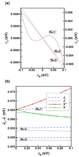
Figure 4: (Color online) Effective interactions (a) $\Lambda_{z}$ and (b) $J_{z},J_{\bot}$ of the Ising quantum Hall valley-ferromagnet as a function of the applied bias for $\widetilde{\nu}=1$ and $N=1,2,3$ at $B=16.5$ T, $\kappa=2.5.$ The interactions $X^{++}$ and $X^{--}$ are also plotted for $N=1.$ In (a) the left axis is for $N=1$ and the right axis for $N=2,3.$

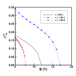
Figure 5: (Color online) Critical bias $\Delta_{B}^{\left(c\right)}$ as a function of the magnetic field in Landau levels $N=1,2$ at $\widetilde{\nu}=1$ for $\kappa=2.5$ and $\kappa=5.$ The region below (above) each curve is valley polarized with $P_{z}=+\frac{1}{2}\left(-\frac{1}{2}\right).$ Biases above $\Delta_{B}^{\left(c\right)}=0.10$ eV are outside the limit of validity of the model.

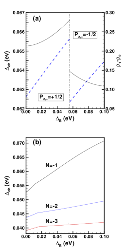
Figure 6: (Color online) (a) Hartree-Fock gap $\Delta_{eh}$ (left axis, black curve) and charge imbalance $\rho_{1}-\rho_{2}$ (right axis, blue dashed curve) plotted as a function of the applied bias for $N=1,B=16.5$ T, $\widetilde{\nu}=1,\kappa=2.5$. Both functions are discontinuous at the transition indicated by the dashed-dotted line. (b) Hartree-Fock gap vs bias for $N=-1,-2,-3$ at $B=10$ T and for $\kappa=2.5.$

VII PHASE DIAGRAM FOR $\widetilde{\nu}=3$

At $\widetilde{\nu}=3,$ the Hartree-Fock energy per electron can be written as

$$\frac{E}{N_{e}}=C^{\prime}-\frac{1}{3}\left[\Lambda_{z}^{\prime}P_{z,-}+J_{z}P_{z,-}^{2}+J_{\bot}P_{\bot,-}^{2}\right],$$ (71)

with $J_{z}$ and $J_{\bot}$ still defined by Eqs. (65) and (66) but with the constant

$$C^{\prime} = \frac{1}{2}\left(E_{-}^{0}+E_{+}^{0}\right)-\frac{3}{4}\alpha_{d}n_{1}n_{2}+\frac{3}{4}\alpha_{d}$$

$$-\frac{5}{24}\Lambda_{z,z}-\frac{1}{6}\Delta_{Z},$$

and the bias term

$$\Lambda_{z}^{\prime} = \left(E_{-}^{0}-\frac{1}{2}X^{\left(-,-\right)}-3\alpha_{d}n_{1,-}n_{2,-}\right)$$

$$-\left(E_{+}^{0}-\frac{1}{2}X^{\left(+,+\right)}-3\alpha_{d}n_{1,+}n_{2,+}\right).$$

The electron-hole symmetry in Landau level $N$ is not perfect since $\Lambda_{z}^{\prime}\neq\Lambda_{z}.$ However, because the terms $\alpha_{d}n_{1,\pm}n_{2,\pm}$ are very small compared to $E_{+}^{0}$ and $X_{N}^{\left(\pm,\pm\right)}$, $\Lambda_{z}^{\prime}\approx$ $\Lambda_{z}$ and the phase diagram for $\widetilde{\nu}=3$ is quasi identical to that for $\widetilde{\nu}=1$.

The C2DEG is thus again an Ising QHF for $\widetilde{\nu}=3$ but with $P_{z,+}$ replaced by $P_{z,-}$. At zero bias, $\Lambda_{z}^{\prime}=0$ and the two ground states $P_{z,-}=\pm\frac{1}{2}$ are degenerate. The charge imbalance is again given by Eq. (68) but with $P_{z,+}$ replaced by $P_{z,-}.$

VIII PHASE DIAGRAM AT $\widetilde{\nu}=2$

For a uniform ground state at $\widetilde{\nu}=2$, numerical calculations show that states with valley and/or spin coherence do not occur. The Hartree-Fock energy per electron can thus be simplified to

$$\frac{E}{N_{e}} = D-\frac{1}{2}\Delta_{Z}S_{z}-J_{z}P_{z}^{{}^{2}}$$

$$-\Lambda_{z}P_{z}-J_{+}S_{z,+}^{2}-J_{-}S_{z,-}^{2},$$

where the constant $D$ is given by

$$D=\frac{1}{2}\left(E_{-}^{0}+E_{+}^{0}+\alpha_{d}-\alpha_{d}n_{1}n_{2}\right)-\frac{1}{4}\left(J_{+}+J_{-}\right),$$ (75)

the effective Heisenberg exchange interactions are

$$J_{z} = \frac{1}{2}\alpha_{d}\left(n_{1,+}-n_{1,-}\right)\left(n_{2,+}-n_{2,-}\right)$$

$$+\frac{1}{4}\left(J_{+}+J_{-}\right),$$

$$J_{\pm} = \frac{1}{2}X^{\left(\pm,\pm\right)},$$ (77)

and the bias term is

$$\Lambda_{z} = -\frac{1}{2}\left(E_{+}^{0}-E_{-}^{0}\right)+\alpha_{d}\left(n_{1,+}n_{2,+}-n_{1,-}n_{2,-}\right)$$

$$+\frac{1}{2}\left(J_{+}-J_{-}\right).$$

In the absence of coherence, the only possible states have $P_{z}=0,\pm 1$ and $S_{z,+},S_{z,-}=\pm\frac{1}{2}.$ However, the sum rule of Eq. (38), which can be rewritten as,

$$\frac{1}{2}-\frac{1}{2}\left|P_{z}\right|^{2}=S_{z,+}^{2}+S_{z,-}^{2}$$ (79)

permits only six combinations. Three of them, with $S_{z}=0,-1,$ must be ruled out since they have higher energies than the state with $S_{z}=1.$ We only need to compare the energies of the three following states to establish the phase diagram:

• Phase 1 is spin polarized and valley unpolarized. It has $S_{z,\pm}=\frac{1}{2},P_{z}=0$ and energy

  $$\frac{E_{1}}{N_{e}}=D-\frac{1}{2}\Delta_{Z}-\frac{1}{4}\left(J_{+}+J_{-}\right).$$ (80)

• Phase 2 is spin unpolarized and valley polarized. It has $S_{z,\pm}=0,P_{z}=+1$ and energy

  $$\frac{E_{2}}{N_{e}}=D-J_{z}-\Lambda_{z}.$$ (81)

• Phase 3 is spin unpolarized and valley polarized. It has $S_{z,\pm}=0,P_{z}=-1$ and energy

  $$\frac{E_{3}}{N_{e}}=D-J_{z}+\Lambda_{z}.$$ (82)

At zero bias, $\Lambda_{z}=0,J_{+}=J_{-}$ and $E_{2}=E_{3}.$ The energy $E_{1}<E_{2},E_{3}$ if the condition $\alpha_{d}\left(n_{1,+}-n_{1,-}\right)^{2}<\Delta_{Z}$ is satisfied, which is always the case. Thus, the ground state is always spin polarized at zero bias. Figures 7 and 8 show the phase diagram for Landau levels $N=1$ and $N=2$ with the dielectric constant $\kappa=2.5.$ The range of bias in these figures is extended beyond the limit of validity of our model in order to show the reentrant spin polarized phase transition that the model would predict. When the bias is increased from zero, phase 1 can make a transition to phase 2 or phase 3. In these figures, the black line with the filled squares separates phase 2 on the left from phase 1 on the right while the blue line with the filled triangles separate phase 1 on the left from phase 3 on the right. Notice that the region corresponding to phase 2 is much smaller for $N=2$ than $N=1.$ For $N=2,$ in most of the phase space, the transition is directly from phase 1 to phase 3.

The transition from phase 1 to phase 2 is exchange-energy driven, just as the pseudospin-flip transition we discussed above for $\widetilde{\nu}=1,3$ was. It does not come from a level crossing. The transition from phase 1 to phase 3, however, is what would be expected from the energy-level diagram of Fig. 2. That is, level $\left(K_{+},+\right)$ crosses level $\left(K_{-},-\right)$ so that the occupied levels in the ground state are $\left(K_{+},+\right),\left(K_{-},+\right)$ in phase 1 and $\left(K_{-},+\right),\left(K_{-},-\right)$ in phase 3. The energy of an occupied level is however strongly modified by the exchange interaction and so the phase transition does not occur at the value given by the crossing of the non-interacting levels which is given by the red dashed line in Figs. 7 and 8 (this line separates phase 1 below from phase 3 above). Comparing the non-interacting and the Hartree-Fock results, one sees that the inclusion of the Coulomb exchange interaction radically changes the phase diagram. This is less so for levels $N<0$ as we show below.

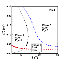
Figure 7: (Color online) Phase diagram in Landau level $N=1$ for filling factor $\widetilde{\nu}=2$ and dielectric constant $\kappa=2.5.$ The red dashed line with the filled red circles is the non-interacting result for the critical bias.

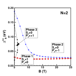
Figure 8: (Color online) Phase diagram in Landau level $N=2$ for filling factor $\widetilde{\nu}=2$ and dielectric constant $\kappa=2.5.$ The red dashed line with the filled red circles is the non-interacting result for the critical bias.

The hopping term $\gamma_{4}$ as well as $\delta_{0}$ that were included in the tight-binding model lead to an electron-hole asymmetry. For this reason, negative Landau levels must be considered separately. Figure 9 shows the phase diagram for $N=-1,-2,-3$ and $\kappa=2.5.$ Phase $2$ is absent from the phase diagram and the predictions of the Hartree-Fock theory is qualitatively the same as those of the non-interacting model obtained from the crossing of the $\left(K_{+},+\right)$ and $\left(K_{-},-\right)$ levels in the energy spectrum. (Note that for $N<0,$ the levels disperse downward in energy instead of upward as in Fig. 2.) The phase diagram for the negative Landau level is obviously not as rich as the one for the positive levels. For $N<0,$ the critical bias evaluated in the absence of Coulomb interaction is bigger than the critical bias found with the Hartree-Fock approximation. For $N>0,$ it is the other way around.

The transition from phase 1 to phase 3 is obtained in the HFA by solving the equation $E_{1}=E_{3}$ i.e.

$$E_{+}^{0}-E_{-}^{0} = \Delta_{Z}-\frac{1}{2}A^{\left(+,+\right)}+\frac{3}{2}A^{\left(-,-\right)}$$

$$-A^{\left(-,+\right)}+J_{+}-J_{-},$$

while the non-interacting result is obtained from $E_{+}^{0}-E_{-}^{0}=\Delta_{Z}.$ The main correction to the non-interacting result comes from the exchange term $J_{+}-J_{-}$.

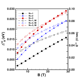
Figure 9: (Color online) Critical bias $\Delta_{B}^{(c)}$ (left axis) and critical electric field $E^{(c)}=\Delta_{B}/d$ (right axis) for the spin polarized to spin unpolarized phase with electrons in valley $K_{-}$ for filling factor $\widetilde{\nu}=2$ and dielectric constant $\kappa=2.5$ in Landau levels $N=-1,-2,-3.$ The dashed lines give the non-interacting results for $\Delta_{B}^{(c)}$ and $E^{(c)}.$

The transport gap $\Delta_{eh}$ and charge imbalance corresponding to Fig. 7 for a magnetic field of $B=10$ T is plotted in Fig. 10. As for the pseudospin-flip transition discussed above for $\widetilde{\nu}=1,3,$ both quantities are discontinuous at the transition. By contrast, Fig. 11 shows that the transport gap is discontinuous at the transition from phase 1 to phase 3 in Landau level $N=1$ for $B<24$ T but is continuous above $B^{\left(c\right)}=24$ T. The gap closes progressively with $B.$ The same situation occurs for $N=2$ where the gap is continuous above $B^{\left(c\right)}=11$ T. The closing of the gap for $N=1,2$ occurs because of a crossing between the two lowest single-particle Hartree-Fock levels. From the matrix $F$ in Eq. (39), the energy of each level is given, in order of increasing energy for $B<B^{\left(c\right)},$ by

$$e_{1} = E_{-}^{0}-\frac{\Delta_{z}}{2}+A^{\left(-,+\right)}+A^{\left(-,-\right)}-X^{\left(-,-\right)},$$ (84)

$$e_{2} = E_{+}^{0}-\frac{\Delta_{z}}{2}+A^{\left(+,+\right)}+A^{\left(+,-\right)}-X^{\left(+,+\right)},$$ (85)

$$e_{3} = E_{-}^{0}+\frac{\Delta_{z}}{2}+A^{\left(-,+\right)}+A^{\left(-,-\right)},$$ (86)

$$e_{4} = E_{+}^{0}+\frac{\Delta_{z}}{2}+A^{\left(+,+\right)}+A^{\left(+,-\right)},$$ (87)

while for $B>B^{\left(c\right)},$ $e_{2}<e_{1}$. The electron-hole gap is thus $\Delta_{eh}=e_{3}-e_{2}$ for $B<B^{\left(c\right)}$ and $\Delta_{eh}=e_{3}-e_{1}$ for $B>B^{\left(c\right)}.$ Using the fact that $E_{1}=E_{3}$ at the transition, it is easy to show analytically that $\Delta_{eh}=0$ for $B>B^{\left(c\right)}.$

The behavior of $\Delta_{eh}$ with bias for $N=-1,-2,-3$ is shown in Fig. 12. The gap has a downward cusp at the transition.

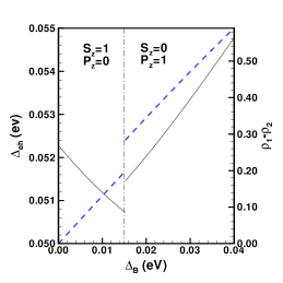
Figure 10: (Color online) Hartree-Fock gap $\Delta_{eh}$ (left axis, full line) and charge imbalance $\rho_{1}-\rho_{2}$ (right axis, dashed line) vs applied bias for $\widetilde{\nu}=2,B=10$ T, $\kappa=2.5$ and $N=1.$ The dashed-dotted line indicates the critical bias for the phase transition.

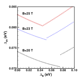
Figure 11: (Color online) Hartree-Fock gap $\Delta_{eh}$ as a function of the applied bias for $\widetilde{\nu}=2$ and $B=20,23,25$ T, $\kappa=2.5,$ $N=1.$

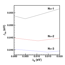
Figure 12: (Color online) Hartree-Fock gap $\Delta_{eh}$ as a function of the applied bias for $\widetilde{\nu}=2,$ $B=10$ T, $\kappa=2.5,$ $N=-1,-2,-3.$

IX DISCUSSION AND CONCLUSION

The experimental study of the C2DEG in BLG has so far been concentrated on the phase diagram in Landau level $N=0$BLGExperiments or to the measurement of the transport gaps between higher Landau levelsExceptions . In a recent publicationTutuc , however, the QHFs that emerge from the quartet of states in Landau levels $N<0$ are studied experimentally (along with the states in $N=0$) using a double bilayer graphene heterostructureTutuc2 . The authors find quantum Hall states at all integer filling factors, which undergo transitions as a function of magnetic and transverse electric fields. At odd filling factors, the QHE is absent at and near zero bias and reemerge at finite bias while at $\widetilde{\nu}=2$ there is a finite critical bias $\Delta_{B}^{\left(c\right)}$around which the QHE is lost.

In a non-interacting picture for the energy levels, the transition at $\widetilde{\nu}=2$ is due to a crossing of the two sublevels $\left(K_{+},+\right)$ and $\left(K_{-},-\right)$ and the ground state changes from a spin polarized to a valley polarized state while the absence of the QHE near zero bias at $\widetilde{\nu}=1$ and $\widetilde{\nu}=3$ is due to the degeneracy of the states $\left(K_{+},+\right)$ and $\left(K_{-},+\right)$ in the former case and $\left(K_{+},-\right)$ and $\left(K_{-},-\right)$ in the latter (see Fig. 2). In this picture the transport gap $\Delta_{eh}$ goes to zero at the level crossing (or degeneracy point), the quantum Hall state is lost and the longitudinal resistance $\rho_{xx}$ increases.

When Coulomb interaction is considered in the Hartree-Fock approximation for Landau levels $N<0$, the gap is finite at all bias but has a downward cusp at the transition between the spin polarized and the valley polarized state at $\widetilde{\nu}=2$ (see Fig. 12) and near zero bias at filling factors $\widetilde{\nu}=1,3$ (see Fig. 6 (b)). If we assume that, in the cusp region the Landau level broadening due to the disorder is larger than the Hartree-Fock gap, then the QHE is lost in this region and the phase transitions found in the HFA are consistent with the experimental results. For this argument to hold, however, the broadening must depend on the Landau level index. Note that the gaps calculated in the Hartree-Fock approximation are exchange-enhanced and so larger than the non-interacting gaps. In fact, they are of the same order than the gap between Landau levels $N$ so that the applicability of no Landau-level mixing approximation seems questionable. However, it was shown previouslyGorbar that static screening can reduce the size of the gaps substantially so that the no mixing approximation can be justified. The inclusion of screening corrections may well modify the phase diagrams discussed in this paper however. As we have shown above, some of the phases like that with $S_{z}=\frac{1}{2},P_{z}=\frac{1}{2}$ for $\widetilde{\nu}=1,3$ and phase 2 ($S_{z}=0,P_{z}=1$) for $\widetilde{\nu}=2$ are sensitive to the value of $\kappa$ and thus to static screening. If these phase disappears with screening, then the phase diagram for $N>0$ will look more like that for $N<0.$ At the moment, there is no data for $N>0$ to which we can compare our results.

In Fig. 3(d) of Ref. Tutuc, , the critical bias $\Delta_{B}^{\left(c\right)}\left(B\right),$ corresponding to observed transition for $\widetilde{\nu}=2,$ is given for $N=0,-1,-2,-3.$ In our terminology, this $\Delta_{B}^{\left(c\right)}\left(B\right)$ corresponds to the transition from phase 1 to phase 3 for which the phase diagram is given in Fig. 9. Qualitatively, our results for $\Delta_{B}^{\left(c\right)}\left(B\right)$ agree well with experiment. The critical bias (or critical electric field) increases almost linearly with magnetic field at small field and it increases with Landau level index $\left|N\right|$ but more slowly as $\left|N\right|$ increases. Quantitatively, the comparison is more difficult because our calculation does not include the disorder which is always present in a real sample. The theoretical critical bias is about eight times smaller than the experimental one depending on the level $N$. As for the slope of $\Delta_{B}^{\left(c\right)}\left(B\right)$ with magnetic field, for $N=-1$ it is $\approx 1.8$ mV$\cdot$nm${}^{-1}\cdot$T^-1 while the experimental result is larger and $\approx 9$ mV$\cdot$nm${}^{-1}\cdot$T^-1. These differences in the slope and value of the critical bias are similar in size to those found between the theoreticalGorbar ; Lambert and experimentalBLGExperiments results for the spin polarized to layer-polarized phase transition that occurs at filling factor $\nu=0$ in level $N=0$ in BLG. Further study is necessary to understand the reason for this discrepancy.

We have, in this work, concentrated our analysis on the uniform states in the phase diagram. The formalism we developped can however be applied to the study of non-uniform states such as charge-density-wave of crystals. We will discuss these states elsewhereDomainwalls together with the charged excitations of the QHF states. Because of the Ising character of the QHF states, the charged excitations can take the form of charged domain wall loops (i.e. Skyrmions)Walls . The transport gap $\Delta_{eh}$ computed in this paper can be modified if these topological excitations have lower energy than the electron-hole pair excitations we considered in this work.

- (1) The Quantum Hall Effect, edited by R. E. Prange and S. M. Girvin (Springer, New York, 1990).
- (2) Perspectives in Quantum Hall Effects, edited by S. Das Sarma, and A. Pinczuk (Wiley, New York, 1996).
- (3) K. Moon, H. Mori, K. Yang, S. M. Girvin, A. H. MacDonald, L. Zheng, D. Yoshioka, and S. C. Zhang, Phys. Rev. B 51, 5138 (1995); K. Yang, K. Moon, L. Belkhir, H. Mori, S. M. Girvin, A. H. MacDonald, L. Zheng, and D. Yoshioka. Phys. Rev. B 54, 11644 (1996).
- (4) Z. F. Ezawa, Quantum Hall Effects (World Scientific, Singapore, 2000).
- (5) M. O. Goerbig, R. Moessner, and B. Douçot, Phys. Rev. B 74, 161407(R) (2006).
- (6) For a review of the C2DEG in bilayer graphene in Landau level , see for example: Yafis Barlas, Kun Yang, and A. H. MacDonald, Nanotechnology 23, 052001 (2012).
- (7) J. Lambert and R. Côté, Phys. Rev. B 87, 115415 (2013).
- (8) Kayoung Lee, B. Fallahazad, J. Xue, T. Taniguchi, K. Watanabe, and E. Tutuc, e-print arXiv:1401.0659v1 [cond-mat.mes.hall].
- (9) Yasuhisa Sakurai and Daijiro Yoshioka, Phys. Rev. B 85, 045108 (2012).
- (10) G. F. Giuliani and J. J. Quinn, Phys. Rev. B 31, 6228 (1985).
- (11) A. J. Daneshvar, C. J. B. Ford, M. Y. Simmons, A. V. Khaetskii, A. R. Hamilton, M. Pepper, and D. A. Ritchie, Phys. Rev. Lett. 79, 4449 (1997).
- (12) T. Jungwirth, and A. H. MacDonald, Phys. Rev. B 63, 035305 (2000).
- (13) For a review of some of the properties of graphene and bilayer graphene, see for example: A. H. Castro Neto, F. Guinea, N. M. R. Peres, K. S. Novoselov and A. K. Geim, Rev. Mod. Phys. 81, 109 (2009); D. S. L. Abergel, V. Apalkov, J. Berashevich, K. Ziegler and Tapash Chakraborty, Advances in Physics 59, 261 (2010); M. O. Goerbig, Rev. Mod. Phys. 83, 1193 (2011);Edward McCann and Mikito Koshino, Rep. Prog. Phys. 76, 056503 (2013).
- (14) R. Côté and Manuel Barrette, Phys. Rev. B 88, 245445 (2013).
- (15) Eduardo V. Castro, K. S. Novoselov, S. V. Morozov, N. M. R. Peres, J. M. B. Lopes dos Santos, Johan Nilsson, F. Guinea, A. K. Geim and A. H. Castro Neto, J. Phys.: Condens. Matter 22, 175503 (2010).
- (16) Edward McCann and Vladimir I. Fal’ko, Phys. Rev. Lett. 96, 086805 (2006).
- (17) R. Côté and A. H. MacDonald, Phys. Rev. B 44, 8759 (1991).
- (18) This is done for Landau level in R. Côté, J. P. Fouquet, and Wenchen Luo, Phys. Rev. B 84, 235301 (2011).
- (19) Benjamin E. Feldman, Jens Martin, and Amir Yacoby, Nat. Phys. 6, 889 (2009); Y. Zhao, P. Cadden-Zimansky, Z. Jiang, and P. Kim, Phys. Rev. Lett. 104, 066801 (2010); R. T. Weitz, M. T. Allen, B. E. Feldman, J. Martin, and A. Yacoby, Science 330, 812 (2010); Seyoung Kim, Kayoung Lee, and E. Tutuc, Phys. Rev. Lett. 107, 016803 (2011); J. Velasco Jr, L. Jing, W. Bao, Y. Lee, P. Kratz, V. Aji, M. Bockrath, C. N. Lau, C. Varma, R. Stillwell, D. Smirnov, Fan Zhang, J. Jung, and A. H. Macdonald, Nat. Nanotechnol. 7, 156 (2012); Seyoung Kim, Kayoung Lee, and E. Tutuc, Phys. Rev. Lett. 107, 016803 (2011); P. Maher, C. R. Dean, A. F. Young, T. Taniguchi, K. Watanabe, K. L. Shepard, J. Hone and P. Kim, Nature Phys. 9, 154 (2013).
- (20) A. S. Mayorov, D. C. Elias, M. Mucha-Kruczynski, R. V. Gorbachev, T. Tudorovskiy, A. Zhukov, S. V. Morozov, M. I. Katsnelson, v. I. Fal’ko, A. K. Geim, K. S. Novoselov, Science 333, 860 (2011); Gregory M. Rutter, Suyong Jung, Nikolai N. Klimov, David B. Newell, Nikolai B. Zhitenev and Joseph A. Stroscio, Nature Phys. 7, 649 (2011); Babak Fallahazad, Yufeng Hao, Kayoung Lee, Seyoung Kim, R. S. Ruoff, and E. Tutuc, Phys. Rev. B 85, 201408(R) (2012).
- (21) Seyoung Kim, Insun Jo, D. C. Dillen, D. A. Ferrer, B. Fallahazad, Z. Yao, S. K. Banerjee, and E. Tutuc, Phys. Rev. Lett. 108, 116404 (2012); Kayoung Lee, Babak Fallahazad, Hongki Min, and Emanuel Tutuc, IEEE transactions on electron devices, 60, 103 (2013).
- (22) E. V. Gorbar, V. P. Gusynin, Junji Jia, and V. A. Miransky, Phys. Rev. B 84, 235449 (2011); E. V. Gorbar, V. P. Gusynin, and V. A. Miransky, JETP Lett. 91, 314 (2010); E. V. Gorbar, V. P. Gusynin, and V. A. Miransky, Phys. Rev. B 81, 155451 (2010); R. Nandkishore and L. Levitov, e-print arXiv: 1002.1966v1 [cond-mat.mes-hall]; C. Töke and V. I. Fal’ko, Phys. Rev. B 83, 115455 (2011).
- (23) Wenchen Luo, R. Côté and Alexandre Bédard-Vallée, unpublished.
- (24) T. Jungwirth, S. P. Shukla, L. Smrčka, M. Shayegan, and A. H. MacDonald, Phys. Rev. Lett. 81, 2328, 1998; T. Jungwirth, A. H. MacDonald, E. H. Rezayi, Physica E 12, 1 (2002); T. Jungwirth and A. H. MacDonald, Phys. Rev. Lett. 87, 216801 (2001).