Metallicity evolution of AGNs from UV emission-lines based on a new index

Abstract

We analyzed the evolution of the metallicity of the gas with the redshift for a sample of AGNs in a very wide redshift range ($0<z<4$) using ultraviolet emission-lines from the narrow-line regions (NLRs) and photoionization models. The new index C43=log[(C iv+C iii])/He ii] is suggested as a metallicity indicator for AGNs. Based on this indicator, we confirmed the no metallicity evolution of NLRs with the redshift pointed out by previous works. We found that metallicity of AGNs shows similar evolution than the one predicted by cosmic semi-analytic models of galaxy formation set within the Cold Dark Matter merging hierarchy (for $z\la 3$). Our results predict a mean metallicity for local objects in agreement with the solar value (12+log(O/H)=8.69). This value is about the same that the maximum oxygen abundance value derived for the central parts of local spiral galaxies. Very low metallicity $\log(Z/Z_{\odot})\approx-0.8$ for some objects in the range $1.5\><\>z\><\>3$ is derived.

1 Introduction

The study of the metallicity in galaxies and the knowledge of the chemical evolution of these objects with the redshift play an important role to understand the formation and evolution of the universe.

In general, models of cosmic chemical evolution predict that the galaxy metallicities increase with the aging of the universe. For example, Malaney & Chaboyer (1996), using neutral hydrogen density obtained from observations of Damped Lyman Alpha objects (DLAs) and an analytic model, showed that, for redshift ($z$) from about 4 to 0, the metallicity ($Z$) rises from $0.05Z_{\odot}$ to 0.6 $Z_{\odot}$. Other models, such as the model of Pei et al. (1999), predict a steeper increase of $Z$ with the cosmological time-scale. From an observational point of view, the relation between the metallicity and the redshift, $Z-z$ relation, is controversial. Along decades, metallicity determinations of DLAs, using mainly the absorption line of the Zn (e.g. Pettini et al. 1994), have been used to test cosmic chemical evolution models (e.g. Kulkarni et al. 2013; Battisti et al. 2012; Somerville et al. 2001; Pei & Fall 1995). Despite the large scattering in the metallicity for a fixed redshift, it has been confirmed the increase of the $Z$ with the time (e.g. Rafelski et al. 2012). The same result is also found by observational studies of the gas phase metallicity of star-forming galaxies (e.g. Maiolino et al. 2008; Savaglio et al. 2005) and by metallicity studies of Narrow-Line Regions (NLRs) of high-$z$ radio galaxies (De Breuck et al., 2000). However, opposite results have also been obtained. For example, Mannucci et al. (2010) from spectroscopic data of star-forming galaxies showed that there is a significant dependence of the gas-phase metallicity on the star-formation rate which, if taken into account, does not yield metallicity evolution with the redshift, at least for $z\><2$.

Moreover, some studies based on emission-lines from active galaxies have failed to identify the cosmic chemical evolution. For example, Dietrich et al. (2003a) compared rest-frame of broad emission-line intensities in the ultraviolet of a sample of 70 quasars ($z\ga 3.5$) with photoionization models results of Hamann et al. (2002). They found that the objects analyzed have an average metallicity of about 4-5 $Z_{\odot}$, which is in disagreement with the $Z$ determinations using absorption lines (see Battisti et al. 2012; Kulkarni et al. 2005). A similar analysis performed by Nagao et al. (2006) using ultraviolet spectra of NLRs for objects with redshifts between 1.2 and 4.0 pointed out a constant behavior of the gas metallicity with $z$. Nagao and collaborators interpreted the lack of evolution of $Z$ obtained from NLRs as a result of the fact that the major epoch of star formation in the host galaxies of active nuclei is at very high redshifts ($z\ga 4$). Also Matsuoka et al. (2009) obtained UV rest-frame spectral data from the narrow-line region of 9 high-z radio galaxies at $z>2.7$ and, combining these with data from the literature, found not significant metallicity evolution in NLRs for $z\la 4$.

Metallicity indicators based on emission-line ratios can be subject to uncertainties (e.g. Dors et al. 2011). In fact, the N v $\lambda$1240/C iv $\lambda$1549 ratio, generally used as metallicity indicator for AGNs (Hamann & Ferland, 1992), can yield $Z$ estimations somewhat uncertain since the $\text{N\,\textsc{v}}$ emission line could be enhanced by Ly$\alpha$ photons scattered in a broad absorption-line wind (see Hamann et al. 2002 and references therein). Moreover, any metallicity indicator based on nitrogen-lines must take into account a N/O abundance relation with the metallicity (Pérez-Montero & Contini, 2009), which is poorly determined for AGNs. In this sense, metallicity indicators based on carbon emission-lines, such as the C iv$\lambda$1549/He ii$\lambda$1640 suggested by Nagao et al. (2006), can be more reliable. Although the relation between C/O abundance ratio and the O/H (used as metallicity tracer) must to be taken into account in calibrations (Garnett et al., 2004), chemical evolution models of QSOs of Hamann & Ferland (1993) predict a C/O abundance ratio nearly constant for objects chemically evolved, i.e older than 1 Gyr. This does decrease the uncertainties in metallicity determinations based on carbon emission-lines.

In this paper, we report an analysis of the chemical evolution of AGNs with the cosmological time-scale by modelling the ultraviolet narrow emission-lines observed at different redshifts. We proposed a new metallicity indicator calibrated taking also into account its dependence on other parameters than the metallicity. The paper is organized as follows. In Section 2 we describe the observational data used along the paper. A description of the photoionization models used in the paper is given in Sect. 3. In Sect. 4 a new metallicity tracer is presented. The results of the use of this index and the discussion are presented in Sects. 5 and 6, respectively. The final conclusions is given in Sect. 7.

2 Observational data

The fluxes of the N v$\lambda$1240, C iv$\lambda$1549, He ii$\lambda$1640, and C iii]$\lambda$1909 emission-lines originated in the NLRs of a sample of Seyfert 2 (12 objects), high-$z$ radio galaxies (59 objects) and type 2 quasars (10 objects) with redshifts $0\la z\la 4.0$ were compiled from the literature. The sample is about the same that the one compiled by Nagao et al. (2006) with the addition of Seyfert 2 data taken from Kraemer et al. (1994) and from Díaz et al. (1988). In Table 1 the identification, redshift, adopted emission-line intensities, and the bibliographic reference of each considered object are presented. The objects in this table are grouped by their nature. We did not consider in our sample the lines with only intensity upper limits reported.

Table 1: Fluxes of emission-lines compiled from the literature.

Seyfert 2
Object	redshift	N v$\lambda$1239	C iv$\lambda$1549	He ii$\lambda$1640	C iii]$\lambda$1909	Flux units ($\rm erg/s/cm^{2}$)	Reference
NGC 1068	0.004	224$\pm 41$	520$\pm 80$	187$\pm 29$	240$\pm 35$	$10^{-14}$	1
NGC 4507	0.012	5.2$\pm 1.0$	13.5$\pm 2.7$	5.6$\pm 1.1$	5.8$\pm 1.2$	$10^{-14}$	1
NGC 5135	0.014	1.1$\pm 0.2$	4.1$\pm 0.8$	10.0$\pm 2.0$	—	$10^{-14}$	1
NGC 5506	0.006	—	4.5$\pm 1.4$	2.0$\pm 0.6$	3.6$\pm 0.7$	$10^{-14}$	1
NGC 7674	0.029	—	11.4$\pm 3.3$	5.1$\pm 1.5$	7.9$\pm 2.7$	$10^{-14}$	1
Mrk 3	0.014	3.0$\pm 1.0$	21$\pm 2$	9$\pm 1$	9$\pm 1$	$10^{-14}$	1
Mrk 573	0.017	6.3$\pm 0.9$	29$\pm 4.3$	12.6$\pm 1.9$	8.8$\pm 1.3$	$10^{-14}$	1
Mrk 1388	0.021	—	8.3$\pm 1.2$	3.8$\pm 0.6$	3.6$\pm 0.5$	$10^{-14}$	1
MCG-3-34-64	0.017	5.0$\pm 0.1$	14$\pm 3$	10$\pm 2$	7$\pm 1$	$10^{-14}$	1
NGC 7674	0.029	—	26$\pm 1.40$	10$\pm 3$	18.36$\pm 6.21$	$10^{-14}$	2
IZw 92	0.037	—	9.7$\pm 2.8$	1.46$\pm 0.43$	—	$10^{-13}$	2
NGC 3393	0.012	1.15	47.75	25.73	—	$10^{-14}$	3
Type 2 Quasar
CDFS-027	3.064	2.5$\pm 0.7$	6.4$\pm 0.5$	2.3$\pm 0.9$	—	$10^{-18}$	1
CDFS-031	1.603	—	24.1$\pm 1.4$	13.3$\pm 1.2$	10.3$\pm 1.3$	$10^{-18}$	1
CDFS-057	2.562	8.4$\pm 1.4$	17.8$\pm 0.8$	7.6$\pm 0.8$	13.3$\pm 0.9$	$10^{-18}$	1
CDFS-112a	2.940	14.6$\pm 0.8$	15.2$\pm 1.0$	8.9$\pm 0.9$	4.5$\pm 0.8$	$10^{-18}$	1
CDFS-153	1.536	—	25.5$\pm 1.4$	6.2$\pm 1.1$	13.7$\pm 1.6$	$10^{-18}$	1
CDFS-202	3.700	26.8$\pm 1.1$	38.9$\pm 1.2$	19.7$\pm 1.5$	—	$10^{-18}$	1
CDFS-263b	3.660	4.6$\pm 0.7$	15.5$\pm 0.8$	—	—	$10^{-18}$	1
CDFS-531	1.544	—	22$\pm 1.4$	17.4$\pm 1.5$	14.4$\pm 1.5$	$10^{-18}$	1
CDFS-901	2.578	6.5$\pm 0.8$	19.7$\pm 1.0$	—	3.3$\pm 0.9$	$10^{-18}$	1
CXO 52	3.288	6$\pm 1.2$	35$\pm 2$	17$\pm 2$	21$\pm 2$	$10^{-18}$	1
High-z radio galaxy
TN J0121+1320	3.517	—	0.263$\pm 0.005$	0.330$\pm 0.012$	0.282$\pm 0.009$	$10^{-16}$	4
TN J0205+2242	3.507	—	0.873$\pm 0.025$	0.519$\pm 0.046$	0.418$\pm 0.049$	$10^{-16}$	4
MRC 0316-257	3.130	—	0.267$\pm 0.011$	0.301$\pm 0.009$	0.345$\pm 0.018$	$10^{-16}$	4
USS 0417-181	2.773	—	0.356$\pm 0.026$	0.492$\pm 0.019$	0.553$\pm 0.047$	$10^{-16}$	4
TN J0920-0712	2.758	1.015$\pm 0.014$	3.365$\pm 0.010$	2.063$\pm 0.011$	1.945$\pm 0.028$	$10^{-16}$	4
WN J1123+3141	3.221	1.698$\pm 0.013$	1.570$\pm 0.011$	0.425$\pm 0.014$	0.183$\pm 0.028$	$10^{-16}$	4
4C 24.28	2.913	1.225$\pm 0.012$	1.235$\pm 0.020$	0.978$\pm 0.011$	0.812$\pm 0.041$	$10^{-16}$	4
USS 1545-234	2.751	1.335$\pm 0.031$	1.343$\pm 0.021$	0.878$\pm 0.012$	0.606$\pm 0.031$	$10^{-16}$	4
USS 2202+128	2.705	0.160$\pm 0.019$	0.704$\pm 0.012$	0.289$\pm 0.010$	0.292$\pm 0.011$	$10^{-16}$	4
USS 0003-19	1.541	—	5.90	3.90	3.40	$10^{-16}$	5
BRL 0016-129	1.589	—	1.60	—	2.60	$10^{-16}$	5
MG 0018+0940	1.586	—	0.81	0.42	0.87	$10^{-16}$	5
MG 0046+1102	1.813	—	0.65	0.55	0.79	$10^{-16}$	5
MG 0122+1923	1.595	—	0.32	0.38	0.32	$10^{-16}$	5
USS 0200+015	2.229	—	4.20	3.20	4.00	$10^{-16}$	5
USS 0211-122	2.336	4.10	5.60	3.10	2.20	$10^{-16}$	5
USS 0214+183	2.130	—	3.00	1.80	1.80	$10^{-16}$	5
MG 0311+1532	1.986	—	0.34	0.20	0.21	$10^{-16}$	5
BRL 0310-150	1.769	—	10.20	4.00	5.00	$10^{-16}$	5
USS 0355-037	2.153	—	2.70	3.70	2.30	$10^{-16}$	5
USS 0448+091	2.037	—	1.20	1.40	2.70	$10^{-16}$	5
USS 0529-549	2.575	—	0.40	0.60	1.80	$10^{-16}$	5
4C 41.17	3.792	—	1.32	0.55	0.91	$10^{-16}$	5
USS 0748+134	2.419	—	1.80	1.50	1.40	$10^{-16}$	5
USS 0828+193	2.572	—	1.90	1.90	2.0	$10^{-16}$	5
4C 12.32	2.468	—	3.40	2.30	1.60	$10^{-16}$	5
TN J0941-1628	1.644	—	3.20	0.90	2.00	$10^{-16}$	5
USS 0943-242	2.923	1.70	3.90	2.70	2.30	$10^{-16}$	5
MG 1019+0534	2.765	0.23	1.04	0.85	0.49	$10^{-16}$	5
TN J1033-1339	2.427	—	2.30	0.80	0.70	$10^{-16}$	5
TN J1102-1651	2.111	—	1.00	1.30	1.10	$10^{-16}$	5
USS 1113-178	2.239	—	1.70	0.70	2.80	$10^{-16}$	5
3C 256.0	1.824	1.40	5.23	5.47	4.28	$10^{-16}$	5
USS 1138-262	2.156	—	0.80	1.30	1.30	$10^{-16}$	5
BRL 1140-114	1.935	—	1.00	0.50	0.60	$10^{-16}$	5
4C 26.38	2.608	—	8.90	5.70	2.40	$10^{-16}$	5
MG 1251+1104	2.322	—	0.30	0.30	0.52	$10^{-16}$	5
WN J1338+3532	2.769	—	1.30	3.00	2.20	$10^{-16}$	5

Table 1: -$continued$

High-z radio galaxy
Object	redshift	N v$\lambda$1240	C iv$\lambda$1549	He ii$\lambda$1640	C iii]$\lambda$1909	Flux units ($\rm erg/s/cm^{2}$)	Reference
MG 1401+0921	2.093	—	0.41	0.50	0.34	$10^{-16}$	5
3C 294.0	1.786	3.10	15.50	15.50	18.60	$10^{-16}$	5
USS 1410-001	2.363	1.68	3.36	2.52	1.12	$10^{-16}$	5
USS 1425-148	2.349	—	2.30	2.30	1.00	$10^{-16}$	5
USS 1436+157	2.538	—	17.0	6.0	9.40	$10^{-16}$	5
3C 324.0	1.208	—	3.67	2.70	3.47	$10^{-16}$	5
USS 1558-003	2.527	—	2.70	1.70	1.20	$10^{-16}$	5
BRL 1602-174	2.043	—	10.0	4.8	2.70	$10^{-16}$	5
TXS J1650+0955	2.510	—	3.20	2.70	1.20	$10^{-16}$	5
8C 1803+661	1.610	—	5.30	2.60	1.90	$10^{-16}$	5
4C 40.36	2.265	—	6.20	5.60	5.90	$10^{-16}$	5
BRL 1859-235	1.430	—	3.40	4.60	4.70	$10^{-16}$	5
4C 48.48	2.343	—	6.10	3.70	2.80	$10^{-16}$	5
MRC 2025-218	2.630	0.62	0.69	0.35	0.97	$10^{-16}$	5
TXS J2036+0256	2.130	—	0.60	0.70	1.20	$10^{-16}$	5
MRC 2104-242	2.491	—	3.80	1.90	2.66	$10^{-16}$	5
4C 23.56	2.483	1.36	2.08	1.52	1.28	$10^{-16}$	5
MG 2121+1839	1.860	—	0.53	0.14	0.24	$10^{-16}$	5
USS 2251-089	1.986	—	3.30	1.30	1.50	$10^{-16}$	5
MG 2308+0336	2.457	0.57	0.63	0.39	0.45	$10^{-16}$	5
4C 28.58	2.891	—	0.30	1.60	1.80	$10^{-16}$	5

References— (1) Data compiled by Nagao et al. (2006), (2) Kraemer et al. (1994), (3) Díaz et al. (1988), (4) Matsuoka et al. (2009),

(5) De Breuck et al. (2000)

Since the emission-line intensities were not reddening corrected it could yield some bias in our results. However, Nagao et al. (2006), using an extinction curve described by Cardelli et al. (1989), showed that the effect of dust extinction on the C iii]/C iv and C iv/He ii emission-line ratios, generally used as ionization parameter and metallicity indicators of AGNs respectively, is not important. It is worth to mention that the data compiled from the literature were obtained with different instrumentation and observational techniques. However, the effects caused by the use of non-homogeneous data, such as the ones used in this work, do not yield any bias on the results of abundance estimations in the gas phase of star-forming regions, as pointed out by Dors et al. (2013).

To investigate possible redshift evolutions of the AGN metallicity based on heterogeneous sample, it is important to verify the effects of the dependence of the metallicity on the AGN luminosity, i.e the $Z-L$ relation (see Matsuoka et al. 2009). For that, we used the He ii$\lambda$1640 luminosity ($L(\rm He\>II)$) as a representative value for the bolometric luminosity, as suggested by Matsuoka et al. (2009). The distance to each object was calculated using the $z$ value given in Table 1 and assuming a spatially flat cosmology with $H_{0}$ = 71 $\rm km\>s^{-1}Mpc^{-1}$, $\Omega_{m}=0.270$, and $\Omega_{\rm vac}=0.730$ (Wright, 2006). In Figure 1 we presented the values of $L(\rm He\>II)$ versus the redshift for the objects in our sample. We computed the average and the standard deviation of the luminosity for 5 redshift intervals and these values are given Table 2 as well as the average values of the observed emission-lines intensities for each interval of redshift considered. We can note the strong dependence of the $L(\rm He\>II)$ with the redshift, probably due to selection effects and that the intrinsic emission-line luminosity of nearby Seyfert 2 galaxies is significantly smaller than that of the high-$z$ radio galaxies and type 2 quasars. Since more luminous AGNs have higher metallicity gas clouds (Matsuoka et al. 2009; Nagao et al. 2006), the $Z-L$ relation must be taken into account in our analysis, in the sense that for high redshift we are analyzing a sample of most metallic objects (more luminous).

Figure 1: Luminosity of He ii$\lambda$1640 versus redshift. The squares represent the values for the objects in Table 1. The circles represent the average and their error bars the standard deviation of the luminosity at each redshift interval (see Table 2).

Table 2: Logarithm of the average values of $L(\rm He\>II)$, the observed UV emission-line intensity ratios for the selected redshift intervals, and the number of objects $N$ included in each interval.

$z$	$N$	$L(\rm He\>II)$ (erg/s)	C iv/He ii	C iii]/C iv	N v/He ii	$\frac{\text{C\,\textsc{iv}}+\text{C\,\textsc{iii]}}}{\text{He\,\textsc{ii}}}$
0-0.1	12	41.71$\pm 0.59$	$0.31\pm 0.27$	$-0.32\pm 0.12$	$-0.47\pm 0.51$	$0.53\pm 0.09$
1.0-2.0	18	42.21$\pm 0.68$	$0.24\pm 0.22$	$-0.14\pm 0.19$	$-0.64\pm 0.07$	$0.46\pm 0.17$
2.0-2.5	22	42.80$\pm 0.35$	$0.10\pm 0.18$	$-0.12\pm 0.27$	$0.01\pm 0.15$	$0.37\pm 0.15$
2.5-3.0	18	42.79$\pm 0.53$	$0.08\pm 0.28$	$-0.14\pm 0.39$	$-0.06\pm 0.28$	$0.37\pm 0.17$
3.0-4.0	8	42.40$\pm 0.49$	$0.25\pm 0.23$	$-0.24\pm 0.37$	$0.07\pm 0.28$	$0.44\pm 0.16$

3 Photoionization models

3.1 Model parameters

In this paper a new metallicity indicator for AGNs is proposed. To obtain a calibration of this indicator with the metallicity, we built photoionization models using Cloudy 08.00 (Ferland et al., 2013). In these models, predicted emission-line intensities depend basically on three parameters, the spectral energy distribution (SED), the ionization parameter $U$ and the metallicity $Z$. In what follows the use of these parameters is discussed.

1. Spectral energy distribution (SED): a two continuum components SED is assumed in the models. One is the Big Bump component peaking at $\rm 1\>Ryd$ with a high-energy and an infrared exponential cut-off, and the other represents the X-ray source that dominates at high energies. This last component is characterized by a power law with a spectral index $\alpha_{x}=-1$. Its normalization was obtained taking into account the value $\alpha_{ox}=-1.4$ assumed for the optical to X-ray spectral index. Models assuming this kind of SED reproduce well a large sample of observational AGN data (see Dors et al., 2012).

2. Ionization parameter $U$: it is defined as $U={\rm Q_{ion}}/4\pi R^{2}_{\rm in}nc$, where ${\rm Q_{ion}}$ is the number of hydrogen ionizing photons emitted per second by the ionizing source, $R_{\rm in}$ is the distance from the ionization source to the inner surface of the ionized gas cloud (in cm), $n$ is the particle density (in $\rm cm^{-3}$), and $c$ is the speed of light. The $U$ value was used as one of the input parameters, therefore, ${\rm Q_{ion}}$ and $R_{\rm in}$ are indirectly defined in each model. Cloudy changes the ${\rm Q_{ion}}$ value when $R_{\rm in}$ is varied for fixed $U$ and $n$ values, that results in the same local cloud properties, yielding homologous models with the same predicted emission-line intensities (Bresolin et al., 1999). We computed a sequence of models with $\log U$ ranging from $-1.0$ to $-3.0$ (using a bin size of 0.5 dex).

   To obtain a representative electron density value for NLRs of AGNs, we compiled from the literature observational intensities of the line ratio of the sulfur [S ii]$\lambda$6717/[S ii]$\lambda$6731 of 53 Seyfert 2 galaxies. Then, we computed the electron density value $n$ for each object using the temden routine of the nebular package of iraf assuming an electron temperature of 10 000 K. In Fig. 2 a histogram of the obtained electron density values is shown. We can see that, for most of the objects, $n$ is lower than about 1200 $\rm cm^{-3}$. The average of these values $<n>=537\>\rm\>cm^{-3}$ was obtained and considered in our models. This value is in consonance with the densities derived by Bennert et al. (2006), who used high-sensitivity spatially-resolved optical spectroscopy of a sample of Seyfert-2 galaxies.

3. Metallicity $Z$: the metallicity of the gas phase in the models was linearly scaled to the solar metal composition with the exception of the N abundance, which was taken from the relation between N/O and O/H given by Dopita et al. (2000). The C/O ratio was considered to be the solar value $\rm\log(C/O)=-0.52$. In the Cloudy code (version 08.00), the value 12+log(O/H)=8.69 taken from Allende Prieto et al. (2001) is assumed as the solar metallicity. The metallicity range $-2.0\>\leq\log(Z/Z_{\odot})\leq\>0.60$ was considered in the models. For models with $\log(Z/Z_{\odot})=0.60$ and $\log U$=$-2.5$, $-3.0$, the predicted intensities of C iv$\lambda$1549 and/or C iii]$\lambda$1909 were about equal to zero and they were not consider in our analysis.

We included internal dust in our models and not match with the observational data was possible, therefore, all models considered in this work are dust free. This result is in agreement with the one derived by Nagao et al. (2006), who showed that dusty models can not explain large observed values of the C iv/He ii line ratio (see also Matsuoka et al. 2009). The reason for models with dust can not explain the observed flux of the lines considered is probably because gas clouds in the high-ionization part of NLRs are dusty free, as suggested by Nagao et al. (2003).

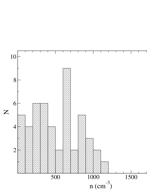
Figure 2: Histogram containing electron density values (in $\rm cm^{-3}$) of Seyfert 2 galaxies calculated using the [S ii]$\lambda 6717/\lambda 6731$ ratio line. The data were taken from Kraemer et al. (1994), Contini et al. (2012), Koski (1978), Cohen (1983), Alloin et al. (1992) Schmitt et al. (1994) Radovich & Rafanelli (1996), Osterbrock (1981), González Delgado & Pérez (1996), Osterbrock & Dahari (1983), Phillips et al. (1983), Goodrich & Osterbrock (1983), Shuder (1980), Durret & Bergeron (1988), and Shuder & Osterbrock (1981).

Table 3: Coefficients of the fitting of $\log(Z/Z_{\odot})=\rm a\times C43^{2}+b\times C43+c$ for different values of $\log U$.

$\log U$	a	b	c
Upper branch
$-$1.0	$-1.45(\pm 0.15)$	$-0.25(\pm 0.16)$	$0.67(\pm 0.04)$
$-$1.5	$-0.59(\pm 0.06)$	$-0.77(\pm 0.03)$	$0.35(\pm 0.01)$
$-$2.0	$-0.18(\pm 0.02)$	$-0.71(\pm 0.03)$	$-0.06(\pm 0.01)$
$-$2.5	$-0.22(\pm 0.02)$	$-0.79(\pm 0.03)$	$-0.38(\pm 0.01)$
$-$3.0	$-0.12(\pm 0.02)$	$-0.71(\pm 0.06)$	$-0.63(\pm 0.03)$
Lower branch
$-$1.0	$4.60(\pm 0.85)$	$-4.03(\pm 1.17)$	$-1.06(\pm 0.39)$
$-$1.5	$4.90(\pm 0.78)$	$-2.53(\pm 0.80)$	$-1.49(\pm 0.19)$
$-$2.0	$1.13(\pm 0.24)$	$1.37(\pm 0.08)$	$-1.70(\pm 0.01)$
$-$2.5	$0.76(\pm 0.18)$	$1.82(\pm 0.10)$	$-1.03(\pm 0.01)$
$-$3.0	$1.02(\pm 0.29)$	$2.81(\pm 0.39)$	$-0.01(\pm 0.11)$

4 C43- A new metallicity tracer

4.1 $Z$-C43 calibration

Several metallicity indicators have been proposed to estimate the metallicity using strong emission-lines from the gas phase of objects without a direct determination of an electron temperature. The idea is basically to calibrate abundances using ratios among the strongest (easily measured) available emission lines. In the case of star-forming regions, the pioneer work by Pagel et al. (1979) proposed the optical metallicity indicator $R_{23}$ (see also Pilyugin et al. 2012). In general, it is preferable to use a line ratio lower dependent on other physical parameters than on the metallicity, for example, a line ratio with a weak dependence on the ionization parameter $U$.

For AGNs, metallicity indicators have also been proposed along decades, for example, using strong optical narrow emission-lines (e.g. Storchi-Bergmann et al. 1998) or UV-lines (see Nagao et al. 2006 and references therein). The main difficult in calibrating an index is that, in general, it depends on metallicity and other parameters, such as the ionization parameter, reddening corrections, electron gas density, abundance ratios (e.g. N/O, C/O; see Hamann & Ferland 1999 for a review). In particular, the C iv/He ii line ratio, suggested by Nagao et al. (2006) as $Z$ indicator, is very dependent on $U$, and a combination of this line ratio with another emission line from an ion with a lower ionization stage than $\rm C^{3+}$ can weakness this dependence. In this sense, we proposed the use of the emission-line ratio C43=log[(C iv+C iii])/He ii] as metallicity indicator. In Fig. 3 the predicted variation of the C43 and C iv/He ii for distinct values of the C/O abundance ratio and ionization parameters, obtained from our models, are shown. It can be noted that, although the behavior of the C43 and the C iv/He ii are very similar respect to the C/O abundances (ranging the interval), a lower variation with the ionization parameter is obtained for C43. The weak dependence of the C43 indicator with the ionization parameter becomes it in a more reliable metallicity indicator than the C iv/He ii. This is analogous to what is obtained in the optical wavelength range for star-forming regions, where the $R_{23}$ parameter is less dependent on the ionization parameter than the [O iii]/H$\beta$ ratio (Kobulnicky et al., 1999). The situation can be different in NLRs of AGNs than in star-forming regions, because free electrons, neutral carbon and $\rm C^{+}$ ions (not considered in C43) can co-exist in an X-ray Dominated Region (see e.g. Mouri et al. 2000). Therefore, the assumption that most of carbon is in the form of $\rm C^{2+}$ or $\rm C^{3+}$ and that the metallicity can be estimated from the line ratio between these ions can be somewhat uncertain. However, even taking this into account, C43 is more reliable than C iv/He ii, since more than one ionization ion stage is considered, tracing a more realistic assumption for the total abundance of C/H.

Figure 3: Bottom panel: Abundance ratio of C/O versus the value of the metallicity indicators C iv/He ii and C43 as indicated. Lines connect the results of our models, represented by points, built considering $\log U=-1.4$, and the other parameters as described in Sect. 4. Top panel- Logarithm of the ionizing parameter versus the value of the metallicity indicators C iv/He ii and C43. A solar metallicity was considered.

In Fig. 4 the calibration between $Z$ and C43 considering different ionization parameter values is shown. In Table 3 the coefficients for second-order polynomial fits to the models is given. We can see that C43 is double-valued with the metallicity, yielding one branch to low metallicity (lower branch) and other to high metallicity (upper branch). This problem is also found for other UV-line ratios (e.g. C iv/He ii, N iv/He ii) and for the $R_{23}$ parameter (see Kewley & Ellison 2008). The inferred metallicities for AGNs, even for the high redshift ones, have been found to be solar or near solar (see e.g. Matsuoka et al. 2009), thus, hereafter we only consider the upper branch along the paper.

Figure 4: Logarithm of the metallicity in relation to the solar one vs. the C43. Curves represent the fits (see Table 3) on model results (represented by points) with distinct ionization parameters as indicated. The hatched area separates the upper and lower branch as indicated.

The ionization parameter can be derived from the C iii]/C iv ratio (Nagao et al., 2006) which is weakly dependent on $Z$, mainly for high values of $U$. In Fig. 5 we show this relation obtained from our models, which is represented by

$$\log U=-0.10(\pm 0.06)\times x^{2}-1.14(\pm 0.02)\times x-1.93(\pm 0.03),$$ (1)

where $x$=log(CIII]/CIV).

Figure 5: Logarithm of the ionization parameter versus log(CIII]/CIV). The points represent the results from our models considering different values for $Z$ and $\log U$. The curve represents a fitting (Eq. 1) to the average points for each $\log U$ value.

4.2 Uncertainties in $Z$ estimations

Uncertainties in $Z$ estimations for star-forming regions based on theoretical and/or empirical calibrations have been addressed for several authors. For example, Kewley & Ellison (2008) showed that different optical methods or different empirical calibrations for the same emission-line ratios provide different oxygen abundances (generally used as $Z$ tracer of the gas phase), with discrepancies up to a factor of 10. Dors et al. (2011), who compared $Z$ estimations based on theoretical diagnostic diagrams and on direct estimations of the electron temperatures, pointed out the importance of combining two line ratios, one sensitive to the metallicity and the other sensitive to the ionization parameter. Regarding uncertainties in $Z$ estimations of AGNs based on UV-lines, few works have addressed this subject. In the case of the C43 index, there are basically four sources of uncertainties, which are discussed in what follows.

1. C/O abundance ratio — Since C43 index is dependent of the C/O abundance, variations in this ratio produce uncertainties in $Z$ determinations. We have performed a simple test to verify these uncertainties. Considering the averaged value for local AGNs (see Table 2) C43=0.53$\pm$0.09, and using the $Z$-C43 calibration for $\log U=-1.5$ presented in Table 3, we obtained $\log(Z/Z_{\odot})=-0.1$. Now, if $\rm\log(C/O)=-0.05$ is assumed to derive a new $Z$-C43 calibration (not shown), we derived $\log(Z/Z_{\odot})=0.20$. Thus, a discrepancy by a factor $\sim$2 is obtained for $Z/Z_{\odot}$.

2. Ionization parameter— As seen in Fig.4, the $Z$-C43 calibration is dependent on $U$. Using the fitting parameters shown in Table 3 and considering that, according to the error in equation 1 and Table 2, $U$ can be estimated with an uncertainty up to 0.5 dex (been about 0.1 for local AGNs), the $Z$ could ranges up to a factor of 3.

3. Observational uncertainties— Considering the observational uncertainty of 0.2 dex in the measured value of C43 and the $Z$-C43 calibration for $\log(U)=-1.5$, we obtained that $\log(Z/Z_{\odot})$ ranges by about a factor of 3.

4. Intrinsic uncertainty— This uncertainty source is associated to the methods that use strong emission-lines to derive the metallicity. Bona fide metallicity determinations for emission-line objects can only be achieved by estimations of the electron temperature ($T_{\rm e}$-method) of the gas phase (see Hägele et al. 2008 and references therein). Therefore, we must compare the $Z$ values for our calibrations with those derived using the $T_{\rm e}$-method. Unfortunately, this was possible only for one object of our sample: NGC 7674. Using the optical data from Kraemer et al. (1994) and adopting the same procedure than Dors et al. (2011) we estimated $\log(Z/Z_{\odot})=-0.22$ for NGC 7674 applying the $T_{\rm e}$-method. $\log U$ for this object, calculated from Eq. 1, is about $-1.7$. Using the correspondent fitting to the $Z$-C43 calibration (see Table 3) we estimated $\log(Z/Z_{\odot})=-0.28$, finding a difference of only 15 per cent between these two estimations. We assumed this difference as representative of the intrinsic uncertainty, even when more data are needed to perform a confident statistical analysis of the influence of this uncertainty on the $Z$-C43 calibration.

Along this paper we consider the derived metallicity from C43 is correct by a factor of 5 (about 0.7 dex), the quadratic sum of the uncertainties discussed above. This discrepancy would be smaller than that given by Kewley & Ellison (2008) for the optical empirical parameters by a factor of 2.

5 Results

In Fig. 6 $\log U$ versus the redshift for the objects in our sample, obtained using Eq. 1, are plotted together with the corresponding average and standard deviation for each redshift bin. We can see that the ionization parameters are in the range $-2.8\>\la\>\log U\>\la-1.0$, with an averaged value of about $-1.75\pm 0.32$ dex. This range is larger than the one found by Nagao et al. (2006), who used the C iv/He ii vs. C iii]/C iv diagnostic diagrams, finding $-2.2\>\la\>\log U\>\la-1.4$.

Figure 6: Logarithm of the ionization parameter vs. the redshift. Squares represent $\log U$ values obtained using Eq. 1 and the observational data presented in Table 1. Circles represent the average and their error bars the standard deviation of $\log U$ for each redshift interval.

To calculate the abundance for each object, we computed the ionization parameter using Eq. 1 and we selected the adequate set of coefficients for the $Z$-C43 calibration (see Table 3) for the closest available $\log U$ value. In Fig. 7 the logarithm of the derived metallicity in relation to the solar one versus the redshift for the objects in our sample for which were possible to estimate $U$ and $Z$ is presented. We can not note any metallicity decrease with the redshift. For some objects it was not possible to estimate $Z$ because some emission-lines needed to calculate C43 were not available. Hence the number of objects plotted in Figs. 7 and 8 is smaller than the one in Table 1 and Fig. 1.

Figure 7: Logarithm of the metallicity in relation to the solar one vs. the redshift. Points represent estimations for the sample presented in Table 1 and considering the $Z$-C43 relations for different values of $\log U$ whose coefficients are given in Table 3. The ionization parameter values were computed using Eq 1.

Figure 8: Such as Fig. 7 but considering different bins of luminosity as indicated in each plot.

Table 4: Average metallicities for the objects in our sample considering different redshift and luminosity ranges. The number of objects in each interval is given. The solar abundance of $\rm 12+\log(O/H)=8.69$ (Allende Prieto et al., 2001) is assumed in the models.

$z$		$\log(Z/Z_{\odot})$	Number
0-0.1	$\log\>L(\rm HeII)\><\>41$	$-0.27(\pm 0.19$)	8
	$41<\log\>L(\rm HeII)\><\>42$	$-0.57(\pm 0.00$)	1
	$42<\log\>L(\rm HeII)\><\>43$	—	—
	$\log\>L(\rm HeII)\>>\>43$	—	—
1.0-2.0	$\log\>L(\rm HeII)\><\>41$	$-0.64(\pm 0.00$)	1
	$41<\log\>L(\rm HeII)\><\>42$	$-0.24(\pm 0.25$)	6
	$42<\log\>L(\rm HeII)\><\>43$	$-0.27(\pm 0.16$)	9
	$\log\>L(\rm HeII)\>>\>43$	$-0.28(\pm 0.05$)	2
2.0-2.5	$\log\>L(\rm HeII)\><\>41$	—	—
	$41<\log\>L(\rm HeII)\><\>42$	—	—
	$42<\log\>L(\rm HeII)\><\>43$	$-0.37(\pm 0.25$)	13
	$\log\>L(\rm HeII)\>>\>43$	$-0.07(\pm 0.19$)	9
2.5-3.0	$\log\>L(\rm HeII)\><\>41$	—	—
	$41<\log\>L(\rm HeII)\><\>42$	$-0.27(\pm 0.40$)	2
	$42<\log\>L(\rm HeII)\><\>43$	$-0.23(\pm 0.35$)	8
	$\log\>L(\rm HeII)\>>\>43$	$-0.16(\pm 0.28$)	8
3.0-4.0	$\log\>L(\rm HeII)\><\>41$	—	—
	$41<\log\>L(\rm HeII)\><\>42$	—	—
	$42<\log\>L(\rm HeII)\><\>43$	$-0.19(\pm 0.12$)	6
	$\log\>L(\rm HeII)\>>\>43$	—	—

In Fig. 8 the $Z$ estimations versus the redshift considering different bins of luminosity is shown. In Table 4 the $Z$ mean values are given. Although none $Z-z$ correlation can be noted, objects with very low metallicity ($\log(Z/Z_{\odot})\approx-0.8$), regardless of the luminosity bin, are only found at redshifts $1\><\>z\><\>3$. In Fig. 9 the metallicity versus the He ii luminosity is presented. The mean values for HzRGs from Matsuoka et al. (2009) are also shown in this plot. Although the large scatter of the points and the no so good linear regression fit to our sample data, it seems to be a slight increase of $Z$ with the He ii luminosity.

Figure 9: Logarithm of the metallicity in relation to the solar one vs. the logarithm of the He ii luminosity. Squares represent estimations for our sample presented in Table 1 and considering the $Z$-C43 relations. Circles represent mean values for HzRGs taken from Matsuoka et al. (2009). A linear regression fit to the data is plotted.

6 Discussion

About two decades ago the first determinations of metallicity in high redshift star-forming galaxies ($z\sim 3$; Kobulnicky & Koo, 2000) and in damped Lyman-$\alpha$ systems ($1.78\><\>z\><\>3$; Pettini et al., 1994) were obtained. From these results, among others, a clear discrepancy arise: luminous high redshift galaxies are more metallic than DLAs at the same redshift (Erb, 2010). Likewise, the metallicity-redshift relation followed by DLAs seems to be in consonance with some cosmic chemical evolution models that predict a $Z$ increment with time (see e.g. Kulkarni et al. 2013). This kind of behavior has not been derived for using estimations of $Z$ for AGNs. With the aim of compare our results with cosmic chemical model predictions and $Z$ determinations for other objects, we plotted them in Fig. 10 as a function of the redshift. In what follows we briefly described the cosmic chemical models shown in this Figure.

1. Malaney & Chaboyer (1996)— Using the redshift evolution of the neutral hydrogen density inferred from observations of DLAs, these authors calculated the evolution of elemental abundances in the Universe based on an analytical model. From this work, models with a mean metallicity value (not corrected for dust obscuration) in a given redshift were considered.

2. Pei et al. (1999)— These authors obtained solutions for the cosmic histories of stars, interstellar gas, heavy elements, dust, and radiation from stars and dust in galaxies using the available data from quasar absorption-line surveys, optical imaging and redshift surveys, and the COBE DIRBE and FIRAS extragalactic infrared background measurements. We considered the mean metallicity of interstellar gas in galaxies predicted by the best models from Pei et al. (1999).

3. Somerville et al. (2001)— They investigated several scenarios for the nature of the high-redshift Lyman-break galaxies using semi-analytic models of galaxy formation set within the cold dark matter merging hierarchy. From the models proposed by these authors, we considered the predictions for the average metallicity of the entire Universe (taken from their Fig. 14), i.e. the total mass in metals divided by total mass of gas. This is the average between the metallicities of the cold gas, stars, hot gas, and diffuse gas.

4. Ballero et al. (2008)– These authors computed chemical evolution of spiral bulges hosting Seyfert nuclei, based on chemical and spectro-photometrical evolution models for the bulge of our Galaxy. We considered the metallicities predicted by those models built assuming a mass of the bulge of $2\>\times\>10^{10}\>M_{\odot}$.

From Fig.10 it can be seen that, for $z\la 3$ and considering the standard deviations, our metallicity estimations are in agreement with the predictions of the cosmic evolution models by Somerville et al. (2001). This agreement confirms the robustness of our $Z$ determinations using the C43 parameter. It also supports the Somerville et al. (2001) assumptions of a hierarchy galaxy formation and the form of the global star formation rate as a function of the redshift. The independence of the metallicity with the redshift derived from our results can be biased by an observational constrain in the way that we are using only the data of luminous objects at high redshift (see Fig. 1), i.e. at such redshifts we are able to observe only the most metallic objects. For $z\>>\>3$, we have few Z determinations and there could be incompleteness effects in the sample. Therefore, definite conclusions can not be obtained for this redshift range.

Models by Malaney & Chaboyer (1996) and Pei et al. (1999) predict higher metallicities than our estimations (see Fig. 10). This could be due to the H i density values used as input in the models of these authors rather than an incorrect selection of the star formation parameters, which control the enrichment of the ISM. The highest discrepancy is found for the model evolution by Ballero et al. (2008), which shows higher values of $Z$ than the ones derived by us. Interestingly, the results from all these chemical evolution models inferred a solar metallicity for the Local Universe, except for the one by Ballero et al. (2008).

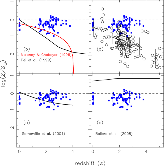
Figure 10: Evolution of the logarithm of the metallicity in solar units $Z/Z_{\odot}$ with the redshift $z$. Squares without error bars represent our metallicity results for AGNs and squares with error bars are the average of our metallicity results and their corresponding standard deviation considering different redshift intervals. In panels (a), (b) and (c), curves represent prediction of cosmic chemical evolution models (see text). In panel (d), circles represent metallicity estimations for Damped L$\alpha$ and sub-Damped L$\alpha$ galaxies via absorption lines by Rafelski et al. (2013), Fox et al. (2007) and Kulkarni et al. (2005), and the circles with error bars represent their mean metallicity values for each redshift interval. Dashed lines represent the solar abundance value.

In panel (d) of Fig. 10, we compare the cosmological mean metallicity ($<Z>$) computed for individual elements (e.g. Zn, S and Si) of DLAs and sub-DLAs (taken from Rafelski et al. 2013, Fox et al. 2007 and Kulkarni et al. 2005) with our metallicity estimations. The abundance solar value is also indicated in this plot. Our results predict a mean metallicity for local objects in agreement with the solar value (12+log(O/H)=8.69). This value is about the same that the maximum oxygen abundance derived for the central parts of spiral galaxies (Pilyugin et al., 2007), and for circumnuclear star-forming regions in both AGNs (Dors et al., 2008) and normal galaxies (Díaz et al., 2007). Concerning the $<Z>$ in DLAs and sub-DLAs, they tend to decrease with the redshift while our estimations for AGNs present an almost flat behavior, showing an agreement only in the Local Universe. Somerville et al. (2001) pointed out that $<Z>$ estimations in DLAs can be systematically underestimated due to two factors. First, dusty high metallicity systems might dim quasars in the line of sight (Pei & Fall, 1995). Second, the outermost regions of spiral galaxies have often lower $Z$ than central regions, thus, $Z$ estimations of objects at high redshift, not spatially resolved, represent values lower than the one attributed to the active nuclei. The $Z$ estimations for the objects in our sample are affected at least by the second factor. Therefore, it is unlikely that the discrepancy found in Fig. 10(d) may be due to the factors discussed by Somerville and collaborators.

As can be seen in Fig. 10, we found no clear metallicity evolution with the redshift. Similar result was also found by Matsuoka et al. (2009) and Nagao et al. (2006). It is worth to emphasize that, independently of the luminosity (see Fig. 8), very low metallicity $Z/Z_{\odot}\approx-0.8$ is found for some AGNs in the range $1.5\><\>z\><\>3$, in consonance with the $<Z>$ found in DLAs and sub-DLAs. Except for the local objects, the mean abundance value estimated by us using the $Z$-C43 calibration is higher than the mean value for DLAs and sub-DLAs for each redshift interval. In fact, Nagao et al. (2006) presented two interpretations from their analysis: (i) the narrow line regions of AGNs have sub-solar metallicities ($-0.7\>\la\>\log(Z/Z_{\odot})\>\la\>0$) if low-density gas clouds with $n\>\la\>10^{3}\>\rm cm^{-3}$ are considered in their photoionization models; (ii) a wider range of gas metallicity ($-0.7\>\la\>\log(Z/Z_{\odot})\>\la\>0.7$) for high-density gas clouds with $n\>\approx\>10^{5}\>\rm cm^{-3}$. Although, in some cases (see e.g. Peterson et al. 2013), high values of electron density (in the order of $10^{5}\>\rm cm^{-3}$) were derived for NLRs, we showed that densities of $\sim 500\>\rm\>cm^{-3}$ are representative for AGNs. This low densities yield that very low metallicity be derived for some objects at high redshift.

7 Conclusions

We proposed here a metallicity indicator based on the emission-line ratio C43=(C iv+ C iii])/He ii. This index seems to be a more reliable metallicity indicator than other proposed in the literature since it has a weak dependence on the ionization parameter. We confirmed the no metallicity evolution of NLRs with the redshift that was pointed out by previous works. Our results predict a mean metallicity for local objects in agreement with the solar value (12+log(O/H)=8.69). This mean value is also in consonance with the maximum oxygen abundance derived for the central parts of spiral galaxies. For $z\la 3$ and considering the standard deviations, our metallicity estimations through the C43 parameter are in agreement with the predictions of the cosmic evolution models by Somerville et al. (2001). For $z\>>\>3$, we have few Z determinations and there could be incompleteness effects in the sample produced by the observational constrain of having data only from the most luminous objects. Therefore, the sample of objects with $z\>>\>3$ is needed to be enlarged, mainly for brightness objects, to avoid possible observational biases and to improved the conclusions about the metallicity evolution of AGNs with the redshift.

References

- Allende Prieto et al. (2001) Alende Prieto, C., Lambert, D. L., Asplund, M. 2001, ApJ, 556, L63
- Allende Prieto et al. (2002) Alende Prieto, C., Lambert, D. L., Asplund, M. 2002, ApJ, 573, L137
- Alloin et al. (1992) Alloin, D., Bica, E., Bonatto, C., Prugniel, P. 1992, A&A, 266, 117
- Baldwin et al. (2003) Baldwin, J. A., Hamann, F., Korista, K. T. et al. 2003, ApJ, 583, 649
- Ballero et al. (2008) Ballero, S. K., Matteucci, F., Ciotti, L., Calura, F., Padovani, P. 2008, A&A, 478, 335
- Battisti et al. (2012) Battisti, A. J., Meiring, J. D., Tripp, T. M. 2012, ApJ, 744, 93
- Becker et al. (2012) Becker, G. D., Sargent, W. L. W., Rauch, M., Carswell, R. F. 2012, ApJ, 744, 91
- Bennert et al. (2006) Bennert, N., Jungwiert, B., Komossa, S., Haas, M., Chini, R. 2006, A&A, 456, 953
- Bresolin et al. (1999) Bresolin, F., Kennicutt, R. C., Garnett, D. R. 1999, ApJ, 510, 104
- Cardelli et al. (1989) Cardelli, J. A., Clayton, G. C., Mathis, J. S. 1989, ApJ, 345, 245
- Contini et al. (2012) Contini, M. 2012, MNRAS, 425, 1205
- Cohen (1983) Cohen, R. D. 1983, ApJ, 273, 489
- De Breuck et al. (2000) De Breuck, C.; Röttgering, H., Miley, G., van Breugel, W., Best, P. 2000, A&A, 362, 519
- Díaz et al. (2007) Díaz, A. I., Terlevich, E., Castellanos, M., Hägele, G. F. 2007, MNRAS, 382, 251
- Díaz et al. (1988) Díaz, A. I., Prieto, M. A., Wamsteker, W. 1988, A&A, 195, 53
- Dietrich et al. (2003a) Dietrich, M., Hamann, F., Shields, J. C. 2003a, ApJ, 589, 722
- Dopita et al. (2000) Dopita, M. A., Kewley, L. J., Heisler, C. A., Sutherland, R. S. 2000, ApJ, 542, 224
- Dors et al. (2013) Dors, O. L., Hagele, G. F., Cardaci, M. V. et al. 2013, MNRAS, 432, 2512
- Dors et al. (2012) Dors, O. L., Riffel, R. A., Cardaci, M. V. et al. 2012, MNRAS, 422, 252
- Dors et al. (2011) Dors, O. L., Krabbe, A., Hägele, G. F., Pérez-Montero, E. 2011, MNRAS, 415, 3616
- Dors et al. (2008) Dors, O. L., Storchi-Bergmann, T., Riffel, R. A., Schimidt, A. A. 2008, A&A, 482, 59
- Durret & Bergeron (1988) Durret, F., & Bergeron, J. 1988, ApJSS, 75, 273
- Erb et al. (2010) Erb, D. K., Pettini, M., Shapley, A. E. et al. 2010, ApJ, 719, 1168
- Erb (2010) Erb, D. K. 2010, Proceedings of the International Astronomical Union, IAU Symposium, 265, 147
- Esteban et al. (2009) Esteban, C., Bresolin, F., Peimbert, M. et al. 2009, ApJ, 700, 654
- Esteban et al. (2005) Esteban, C., García-Rojas, J., Peimbert, M. et al. 2005, ApJ, 618, L95
- Esteban et al. (2004) Esteban, C., Peimbert, M., García-Rojas, J., et al. 2004, MNRAS, 355, 229
- Esteban et al. (2002) Esteban, C., Peimbert, M., Torres-Peimbert, S., Rodr guez, M. 2002, ApJ, 581, 241
- Ferland et al. (2013) Ferland, G. J., Porter, R. L., van Hoof, P. A. M. et al. 2013, Rev. Mexicana Astron. Astrofis., 49, 137
- Fox et al. (2007) Fox, A. J., Ledoux, C., Petitjean, P., Srianand, R. 2007, A&A, 473, 791
- Garnett et al. (2004) Garnett, D. R., Edmunds, M. G. et al. 2004, AJ, 128, 2772
- Garnett et al. (1997) Garnett, D. R., Shields, G. A., Skillman, E. D., Sagan, S. P., Dufour, R. J. 1997, ApJ, 489, 63
- Garnett et al. (1995) Garnett, D. R., Skillman, E. D., Dufour, R. J. et al. 1995, ApJ, 443, 64
- González Delgado & Pérez (1996) González Delgado, R. M., & Pérez, E. 1996, MNRAS, 281, 1105
- Goodrich & Osterbrock (1983) Goodrich, R. W., & Osterbrock, D. 1983, ApJ, 269, 416
- Guseva et al. (2011) Guseva, N. G., Izotov, Y. I., Stasińska, G. et al. 2011, A&A, 529, 149
- Hägele et al. (2012) Hägele, G. F., Firpo, V., Bosch, G., Díaz, A. I., Morrell, N. 2012, MNRAS, 422, 3475
- Hägele et al. (2011) Hägele, G. F., García-Benito, R., Pérez-Montero, E. et al. 2011, MNRAS, 414, 272
- Hägele et al. (2008) Hägele G. F., Díaz A. I., Terlevich E., Terlevich R., Pérez-Montero E., Cardaci M. V., 2008, MNRAS, 383, 209
- Hamann et al. (2002) Hamann, F., Korista, K. T., Ferland, G. J., Warner, C., Baldwin, J. 2002, ApJ, 564, 592
- Hamann & Ferland (1999) Hamann, F., & Ferland, G. J. 1999, 1999, ARA&A, 37, 487
- Hamann & Ferland (1993) Hamann, F., & Ferland, G. J. 1993, ApJ, 418, 11
- Hamann & Ferland (1992) Hamann, F., & Ferland, G. J. 1992, ApJ, 391, L53
- Holweger (2001) Holweger, H., 2001, AIP Conference Proceedings, Vol. 598, pp.23-30
- Izotov et al. (2006) Izotov, Y. I., Stasińska, G., Meynet, G., Guseva, N. G., Thuan, T. X. 2006, A&A, 448, 955
- Kewley & Ellison (2008) Kewley, L. J., Ellison, S. L. 2008, 681, 1183
- Kobulnicky & Koo (2000) Kobulnicky, H. A., & Koo, D. C. 2000, ApJ, 545, 712
- Kobulnicky et al. (1999) Kobulnicky, H. A., Kennicutt, R. C., Pizagno, J. L. 1999, ApJ, 514, 544
- Kobulnicky & Skillman (1998) Kobulnicky, H. A., Skillman, E. D. 1998, ApJ, 497, 601
- Koski (1978) Koski, A. T. 1978, ApJ, 223, 56
- Kraemer et al. (1994) Kraemer, S. B., Wu, C.-C., Crenshaw, D. M., Harrington, J. P. 1994, ApJ, 435, 171
- Kulkarni et al. (2013) Kulkarni, G., Rollinde, E., Hennawi, J. F., Vangioni, E. 2013, ApJ, 772, 93
- Kulkarni et al. (2005) Kulkarni, V. P., Fall, S. M., Lauroesch, J. T. et al. 2005, ApJ, 618, 68
- Maiolino et al. (2008) Maiolino, R., Nagao, T., Grazian, A. et al. 2008, A&A, 488, 463
- Malaney & Chaboyer (1996) Malaney, R. A., & Chaboyer, B. 1996, ApJ, 462, 57
- Mannucci et al. (2010) Mannucci, F., Cresci, G., Maiolino, R., Marconi, A., Gnerucci, A. 2010, MNRAS, 408, 2115
- Matsuoka et al. (2009) Matsuoka, K., Nagao, T., Maiolino, R., Marconi, A., Taniguchi, Y. 2009, A&A, 503, 721
- Mouri et al. (2000) Mouri, H., Kawara, K., Taniguchi, Y. 2000, ApJ, 528, 186
- Nagao et al. (2006) Nagao, T., Maiolino, R., Marconi, A. 2006, A&A, 447, 863
- Nagao et al. (2003) Nagao, T., Murayama, T., Shioya, Y., Taniguchi, Y. 2003, AJ, 125, 1729
- Osterbrock & Dahari (1983) Osterbrock, D. E., & Dahari, O. 1983, ApJ, 273, 478
- Osterbrock (1981) Osterbrock, D. E. 1981, ApJ, 249, 462
- Pagel et al. (1979) Pagel, B. E. J., Edmunds, M. G., Blackwell, D. E., Chun, M. S., Smith, G. 1979, MNRAS, 189, 95
- Pei et al. (1999) Pei, Y. C., Fall, S. M., Hauser, M. G. 1999, ApJ, 522, 604
- Pei & Fall (1995) Pei, Y. C., & Fall, S. M. 1995, ApJ, 454, 69
- Pérez-Montero et al. (2011) Pérez-Montero, E., Vílchez, J. M., Cedrés, B. et al. 2011, A&A, 532, 141
- Pérez-Montero & Contini (2009) Pérez-Montero, E., & Contini, T. 2009, MNRAS, 398, 949
- Peterson et al. (2013) Peterson B. M., Denney, K. D., De Rosa, G. et al., 2013, ApJ, 779, 109
- Pettini et al. (1994) Pettini, M., Smith, L. J., King, Hunstead, R. W., King, D. L. 1994, ApJ, 426, 79
- Pilyugin et al. (2012) Pilyugin, L. S., Grebel, E. K., Mattsson, L. 2012, MNRAS, 424, 2316
- Pilyugin et al. (2007) Pilyugin, L. S., Thuan, T. X., Vílchez, J. M. 2007, MNRAS, 376, 353
- Phillips et al. (1983) Phillips, M. M., Charles, P. A., Baldwin, J. A. 1983, ApJ, 266, 485
- Radovich & Rafanelli (1996) Radovich, M., & Rafanelli, P. 1996, A&A, 306, 97
- Rafelski et al. (2013) Rafelski, M., Neeleman, M., Fumagalli, M., Wolfe, A. M., Prochaska, J. X. 2013 arXiv, arXiv:1310.6042
- Rafelski et al. (2012) Rafelski, M., Wolfe, A. M., Prochaska, J. X., Neeleman, M., Mendez, A. J. 2012, ApJ, 755, 89
- Savaglio et al. (2005) Savaglio, S., Glazebrook, K., Le Borgne, D. et al. 2005, ApJ, 635, 260
- Shapley et al. (2003) Shapley, A. E., Steidel, C. C., Pettini, M., Adelberger, K. L. 2003, ApJ, 588, 65
- Schmitt et al. (1994) Schmitt, H. R., Storchi-Bergmann, T., Baldwin, J. A. 1994, ApJ, 423, 237
- Somerville et al. (2001) Somerville, R. S., Primack, J. R., Faber, S. M. 2001, MNRAS, 320, 504
- Storchi-Bergmann et al. (1998) Storchi-Bergmann, T, Schmitt, H. R., Calzetti, D., Kinney, A. L. 1998, AJ, 115, 909
- Shuder (1980) Shuder, J. M. 1980, ApJ, 240, 32
- Shuder & Osterbrock (1981) Shuder, J. M., & Osterbrock, D. E. 1981, ApJ, 250, 55
- Wright (2006) Wright, E. L. 2006, PASP, 118, 1711